Journal of Computational and Applied Mathematics 224 (2009) 152–167

Contents lists available at ScienceDirect

Journal of Computational and AppliedMathematics

journal homepage: www.elsevier.com/locate/cam

A generalization of the Runge–Kutta iterationR. Haelterman a,∗, J. Vierendeels b, D. Van Heule aa Royal Military Academy, Department of Mathematics (MWMW), Renaissancelaan 30, B-1000 Brussels, Belgiumb Ghent University, Department of Flow, Heat and Combustion Mechanics, St.-Pietersnieuwstraat 41, B-9000 Gent, Belgium

a r t i c l e i n f o

Article history:Received 16 March 2007

MSC:65F1065N55

Keywords:Iterative solutionMulti-gridMulti-stage

a b s t r a c t

Iterative solvers in combination with multi-grid have been used extensively to solve largealgebraic systems. One of the best known is the Runge–Kutta iteration. We show thata generally used formulation [A. Jameson, Numerical solution of the Euler equations forcompressible inviscid fluids, in: F. Angrand, A. Dervieux, J.A. Désidéri, R. Glowinski (Eds.),Numerical Methods for the Euler Equations of Fluid Dynamics, SIAM, Philadelphia, 1985,pp. 199–245] does not allow to form all possible polynomial transmittance functions andwe propose a new formulation to remedy this, without using an excessive number ofcoefficients.After having converted the optimal parameters found in previous studies (e.g. [B.

Van Leer, C.H. Tai, K.G. Powell, Design of optimally smoothing multi-stage schemes forthe Euler equations, AIAA Paper 89–1923, 1989]) we compare them with those that weobtain when we optimize for an integrated 2-grid V -cycle and show that this resultsin superior performance using a low number of stages. We also propose a variant ofour new formulation that roughly follows the idea of the Martinelli–Jameson scheme[A. Jameson, Analysis and design of numerical schemes for gas dynamics 1, artificialdiffusion, upwind biasing, limiter and their effect onmultigrid convergence, Int. J. Comput.Fluid Dyn. 4 (1995) 171–218; J.V. Lassaline, Optimal multistage relaxation coefficientsfor multigrid flow solvers. http://www.ryerson.ca/~jvl/papers/cfd2005.pdf] used on theadvection–diffusion equationwhich that can be extended to other types. Gains in the orderof 30%–50% have been shown with respect to classical iterative schemes on the advectionequation. Better results were also obtained on the advection–diffusion equation than withthe Martinelli–Jameson coefficients, but with less than half the number of matrix-vectormultiplications.

© 2008 Elsevier B.V. All rights reserved.

1. Introduction

Euler/Navier–Stokes solvers have long been using explicit multi-stage time-marching schemes because of theirsimplicity. Acceleration techniques like multi-grid have been successfully added, which depend heavily on the smoothingproperties of the multi-stage scheme. Despite its simplicity, the one-dimensional wave equation has been used as a modelwith remarkably good results to find optimal coefficients for real flow solvers for the Euler or Navier–Stokes equations. Oneof themain reasons is the observation that the locus of the one-dimensional scalar Fourier symbol of the advection equationforms the envelope of the loci of the eigenvalues of the discretization matrix of the two-dimensional Euler equations ifblock-Jacobi preconditioning is used [4,5]. For that reason we focus on this simple equation.

∗ Corresponding author. Tel.: +32 2 742 6527; fax: +32 2 742 6512.E-mail addresses: Robby.Haelterman@rma.ac.be (R. Haelterman), Jan.Vierendeels@UGent.be (J. Vierendeels), Dirk.Van.Heule@rma.ac.be

(D. Van Heule).

0377-0427/$ – see front matter© 2008 Elsevier B.V. All rights reserved.doi:10.1016/j.cam.2008.04.021

R. Haelterman et al. / Journal of Computational and Applied Mathematics 224 (2009) 152–167 153

It has already been discovered [5] that coefficients that optimize the smoothing properties of a multi-stage scheme usedin conjunction with multi-grid does not automatically result in the fastest overall performance. To find out why this is,we extend the Fourier analysis to other components of an idealized two-grid V -cycle (restriction, defect correction andprolongation) and look at the resulting transmittance for which we try and find the optimal set of coefficients.This paper is organized as follows. In Sections 2 and 3 we give a brief introduction on multi-stage solvers of the

Runge–Kutta type; in Section 4 we propose our alternative formulation; in Section 5 we detail the different objectivefunctions that we use in the optimization procedure and discuss the results which show that this integrated approach givesimproved convergence speeds, but also show that a high number of stages is not necessarily beneficial. Finally, in Section 6,we introduce a variant that splits the discretization matrix in its Hermitian and anti-Hermitian part and show that furtherimprovements can be obtained.

Remark. We use i as a symbol for the complex unit (=√−1) and i as an index.

2. Iterative solution of an algebraic system of linear equations

We want to solve a linear algebraic system of the type

Au = b (1)

where A ∈ Rp×p;u, b ∈ Rp×1, which typically results from the discretization of a linear ordinary (or partial) differentialequation; we will go into more detail in Section 5. If the dimension of the above system becomes too large, the solutionis often found in an iterative way. The subclass of iterative solvers that we consider here starts from a regular splitting ofA : A = M − N whereM is regular. This results in

un+1 = M−1Nun +M−1b (2)

starting from an initial guess uo, or, after rearranging the terms,

un+1 = un −M−1rn (3)

where we call rn = Aun − b the residual at iteration n. The splitting that will concern us most in this paper is that with

M =1τIp (4)

where Ip ∈ Rp×p is the identity matrix and τ is an iteration parameter. With a fixed value of τ this scheme is called thestationary Richardson iteration. It is obvious that it corresponds to

un+1 = un − τ (Aun − b) (5)

which can be interpreted as stemming from a time discretization, with a (pseudo-) time-step τ ):

un+1 − unτ

+ Aun = b (6)

where we assume that we are only interested in the steady state solution. In the following paragraphs we build upon thissingle-stage iterative scheme to construct the various multi-stage schemes. In Section 6 we will consider yet other ways tosplit A.

3. The Runge–Kutta time-stepping scheme

The Runga–Kutta (R–K) scheme can be implemented for a scalar time-stepping scheme. In a commonly usedmatrix formit is given by

U(o) = unU(1) = U(o) − α1M−1r(o)...

U(l+1) = U(o) − αl+1M−1r(l)...

U(m) = U(o) − αmM−1r(m−1)un+1 = U(m)

(7)

154 R. Haelterman et al. / Journal of Computational and Applied Mathematics 224 (2009) 152–167

where α1, . . . , αm are the iteration parameters. We can write un = uexact + en, where en is the error of un with respect tothe exact solution uexact = A−1b.After some algebra we find

en+1 = Pm(−M−1A)en (8)

where the transmittance function Pm is given by the polynomial

Pm(z) = 1+m∑l=1

(m∏

i=m−l+1

αi

)z l (9)

= 1+m∑l=1

βlz l (10)

with βl =∏mi=m−l+1 αi.

Let σ(M−1A) = {λ1, . . . , λp} denote the spectrum of M−1A. We assume that M−1A has p distinct orthonormaleigenvectors Ei, corresponding to eigenvalues λi (i = 1, . . . , p), so that every error en can be written as a linear combinationof these eigenvectors (en =

∑pi=1(en)i =

∑pi=1(an)iEi). Due to the linear nature of the equations we only need to consider

one component at a time and write

(en+1)i = Pm(−λi)(en)i. (11)

In order to have a stable scheme we require that

|Pm(−λi)| ≤ 1 (∀i ∈ {1, . . . , p}). (12)

The main limitation of the Runge–Kutta solver in this formulation is that the following statement holds

∃l < m : βl = 0⇒ ∀k ∈ {l+ 1, l+ 2, . . . ,m} : βk = 0. (13)

Remark. Other formulations exist, e.g. in [2], but these usem+ (m− 1)! coefficients to form a polynomial of degreem andrequire more storage.

4. An alternative Runge–Kutta formulation

To avoid the limitation (13) of the Runge–Kutta schemewe propose the following formulation, which can be interpretedas a periodic non-stationary method [12].

U(o) = unV(o) = M−1r(o)U(1) = U(o) − γ1V(o)V(1) = −M−1AV(o)U(2) = U(1) − γ2V(1)V(2) = −M−1AV(1)...

V(l) = −M−1AV(l−1)U(l+1) = U(l) − γl+1V(l)...

V(m−1) = −M−1AV(m−2)U(m) = U(m−1) − γmV(m−1)un+1 = U(m)

(14)

where γ1, . . . , γm are the iteration parameters. This results in

en+1 = P ′m(−M−1A)en (15)

(en+1)i = P ′m(−λi)(en)i (i = 1, . . . , p) (16)

R. Haelterman et al. / Journal of Computational and Applied Mathematics 224 (2009) 152–167 155

where

P ′m(z) = 1+m∑l=1

γlz l. (17)

It is easy to see that any real m-th degree polynomial respecting P ′m(0) = 1 can be constructed in this way, thus avoidingthe limitation in (13).If ∀λi ∈ σ(M−1A) : Pm(λi) = P ′m(λi) Eqs. (9) and (17) then the coefficients αl and γl(l = 1, . . . ,m) are related by the

following expressionm∏

m−l+1

αi = γl (l = 1, . . . ,m). (18)

We see that in this new formulation intermediate results need not be stored which reduces storage cost. Another addedbenefit of the scheme is that it uses the coefficients of the transmittance polynomial directly which will result in fewerrounding errors when finite precision coefficients are used, whereas for (9) it is obtained by multiplication. From Eq. (17)we also see that

P ′m(−M−1A) = Ip +

(m∑l=1

γl(−M−1A)l−1)(−M−1A). (19)

We can thus interpret the above equation as a preconditioned form of (3), where the polynomial preconditioner is given by∑ml=1 γl(−M

−1A)l−1.

5. Optimization of parameters

5.1. The equations under consideration

We now try to find the optimal parameters γl (l = 1, . . . ,m) for the one-dimensional advection equation

∂u∂t+ a

∂u∂x= 0 (20)

(a ∈ R+o ) with suitable boundary conditions. We are only interested in the steady-state solution of Eq. (20). The spatialderivative is discretized with a first or second order upwind scheme (resp. U1 and U2) or a K3 upwind biased scheme.With the mesh size given by∆x, the discretization of the space operator ∂u

∂x (on a regular mesh) gives• U1

uj − uj−1∆x

(21)

• U23uj − 4uj−1 + uj−2

2∆x(22)

• K32uj+1 + 3uj − 6uj−1 + uj−2

6∆x. (23)

To study the behavior of the iterative scheme when using the resulting discretization matrix, we pass from the discreterepresentation of the p eigenvalues to the continuous representation given by the Fourier symbol λ(θ), (θ ∈ [−π, π]). VonNeumann analysis then shows that it is given by• U1

λ(θ) =1− e−iθ

∆x(24)

• U2

λ(θ) =3− 4e−iθ + e−2iθ

2∆x(25)

• K3

λ(θ) =3+ 2eiθ − 6e−iθ + e−2iθ

6∆x. (26)

156 R. Haelterman et al. / Journal of Computational and Applied Mathematics 224 (2009) 152–167

5.2. Objective functions

With every θ ∈ [−π, π] we associate an eigenvalue λ(θ) and an eigenvector Eθ . We use (en)θ for the correspondingcomponent of en. This allows us to write

(en+1)θ = P ′m(−λ(θ))(en)θ . (27)

The eigenvector corresponding to the eigenvalue 0 is the ‘‘constant vector’’ (= [1 1 . . . 1]T), which we assume to beeliminated due to the presence of boundary conditions.While it is possible to find coefficients that allow this equation to be solved with (14) it will always suffer from very slow

convergence, as for values of θ for which λ(θ) ≈ 0 we will have P ′m(−λ(θ)) ≈ 1. For that reason we turn our attention tomulti-grid schemes, and use (14) as a smoother.We recall that there are two ways to define ‘‘smooth’’ errors. In geometrical multi-grid, these are the errors that vary

slowly over the grid, i.e. those with θ ∈ ΦLF = [−π2 ,

π2 ]. In algebraic multi-grid, ‘‘smooth’’ denotes the errors that cannot

easily be reduced by the smoother, i.e. those with λ(θ) ≈ 0. In this paper we will limit ourselves to geometrical multi-grid;as for the equations under considerations both approaches are similar.When looking for good coefficients in this contextwewant a scheme that adequately reduces errors forwhich θ ∈ ΦHF =

[−π, π] \ ΦLF . We define the smoothing factor ρHF as

ρHF = supθ∈ΦHF

|P ′m(−λ(θ))|. (28)

A first objective function to minimize would simply be

I1 = ρHF (29)

which depends on the coefficients γ1, . . . , γm. We add the stability constraint

supθ∈[−π,π ]

|P ′m(−λ(θ))| ≤ 1. (30)

This objective function is the one used in most previous studies (e.g. [1,11]) and means that we ignore the effect of theremainder of the multi-grid cycle. Additionally, [11] required that the polynomial had a number of zeroes in the highfrequency domain.We could refine this objective function by adding the effect of the defect correction. We consider a two-grid V -cycle,

where we assume that the solution on the coarser grid (defect correction) is exact (ideal two-grid cycle). This does notnecessarily mean that all errors corresponding to θ ∈ ΦLF will be completely annihilated, as due to the restriction andprolongation process (which act as non-ideal low-pass filters) some high frequencies will be passed to the coarse grid(aliasing), while the low frequencies will be attenuated. Wewill only quantify the latter effect, ignoring aliasing. We use fullweighting for the restriction and linear interpolation for the prolongation. Their effect can be quantified by the followingtransmittance functions (resp. for the restriction and prolongation) that act on the residual [3]

µR =14

(eiθ + 2+ e−iθ

)(31)

=

(cos

θ

2

)2(32)

µP = µR. (33)

Thismeans that even the best defect correctionwill only be able to reduce a fraction of the low frequency part of the residual,which is given by

rn = Aen (34)(rn)θ = A(en)θ = λ(θ)(en)θ . (35)

The resulting objective function then becomes

I2 = supθ∈[−π,π ]

∣∣µV ,1(θ)∣∣ (36)

where

µV ,1(θ) =

(1−

(cos

θ

2

)4) (P ′m(−λ(θ))

)2 for θ ∈ ΦLF (37)

(P ′m(−λ(θ))

)2 for θ ∈ ΦHF . (38)

(Minimizing I2 will automatically take into account the stability constraint I2(θ) ≤ 1,∀θ ∈ [−π, π].)

R. Haelterman et al. / Journal of Computational and Applied Mathematics 224 (2009) 152–167 157

Fig. 1.∣∣∣ 2λ(θ)λ(2θ)

∣∣∣ for the advection equation; different discretization schemes.Using this objective function means that we take a pre-smoothing step followed by an idealized defect correction, that is

only limited by the filtering done by restriction and prolongation, and finally a post-smoothing step. Using the coefficientsthat minimize this function will lead to a smoother that will sacrifice damping of the high frequencies for a better resolutionof the somewhat lower frequencies. Due to the fact that the stability constraint is now taken over the whole V -cycle, it isalso quite possible that the smoother itself is not stable.A last refinement with a respect to the previous objective function takes into account the limitations of the defect

correction itself. Even if we consider a direct solver on the coarsest grid, which is the ideal situation, it is limited by its abilityto eliminate the low frequency errors if we use a similar discretization scheme on the coarsest grid. If we use a coarse gridspacing of 2∆x, this can be quantified by the Fourier symbol on the coarsest grid which is given by λ(2θ)2 (θ ∈ [−π

2 ,π2 ]) [3].

The solution process on the coarsest grid then computes

λ(2θ)2

(vθ )coarse = (rθ )coarse = λ(θ) (eθ )coarse(θ ∈

[−π

2,π

2

])(39)

where (vθ )coarse stands for the defect correction on the coarse grid, and (rθ )coarse ((eθ )coarse) for the value of the residual(error) on the coarse grid, after restriction. 2λ(θ)

λ(2θ) is then a measure of how well the coarse grid operator can resolve the lowfrequencies. We finally propose our third objective function

I3 = supθ∈[−π,π ]

∣∣µV ,2(θ)∣∣ (40)

where

µV ,2(θ) =

(1−

(cos

θ

2

)4 2λ(θ)λ(2θ)

) (P ′m(−λ(θ))

)2 for θ ∈ ΦLF (41)

(P ′m(−λ(θ))

)2 for θ ∈ ΦHF . (42)

Again the minimization procedure will result in I3(θ) ≤ 1,∀θ ∈ [−π, π] if an optimum exists.The last two objective functions (I2 andI3)will generally result inmulti-stage schemes that are not as good as smoothers,

but give a better overall performance after one complete V -cycle. Also note thatwe are in effectminimizing a spectral radius,which means that we are optimizing the asymptotic rate of convergence [12].To illustrate the effect of 2λ(θ)

λ(2θ) for the advection equation, we plot this ratio for U1,U2 and K3 in Fig. 1. We see that thisresults in a slight over-correction for U1 and amore pronounced over-correction for K3. For U2 the ratio approximates unityquite closely over a wide range of values of θ , but with a slight under-correction.In itself, over-correction is not necessarily a bad thing, as it compensates for the filtering done by the restriction and the

prolongation. For that reason we also look at(1−

(cos θ2

)4 2λ(θ)λ(2θ)

)for the three schemes and see (Fig. 2) that all three have

difficulties reducing errors around θ = π2 , which is most pronounced for K3. However, K3 manages to reduce errors close

to θ = 0 best.

5.3. Results

To find the optimal parameters for the different objective functions a routine was written in Matlab 7 that creates alarge number of random seed vectors, containing initial guesses for the various parameters. These are then fed to another

158 R. Haelterman et al. / Journal of Computational and Applied Mathematics 224 (2009) 152–167

Fig. 2.∣∣∣1− (cos θ2 )4 2λ(θ)λ(2θ)

∣∣∣ for the advection equation; different discretization schemes.Table 1Optimalm-stage coefficients for I1

m = 1 m = 2 m = 3 m = 4 m = 5 m = 6

γ1 0.5000 1.0000 1.5000 2.0000 2.5000 3.0000γ2 0.3333 0.9000 1.7060 2.7588 4.0608γ3 0.2000 0.7059 1.6380 3.1211γ4 0.1176 0.5172 1.4242γ5 0.0689 0.3636γ6 0.0404m√

I1 0.7078 0.5786 0.5226 0.4941 0.4780 0.47852m√

I2 0.7056 0.6651 0.7179 0.7566 0.7849 0.80662m√

I3 0.7056 0.7159 0.7703 0.8071 0.8329 0.85212m√

IE 0.6267 0.7171 0.7702 0.8075 0.8333 0.8525

Advection equation using U1 after conversion from [11].

Table 2Optimalm-stage coefficients for I1

m = 2 m = 3 m = 4 m = 5 m = 6

γ1 0.4693 0.6936 0.9214 1.1508 1.3805γ2 0.0934 0.2371 0.4289 0.6701 0.9649γ3 0.0315 0.1028 0.2235 0.4063γ4 0.0103 0.0412 0.1057γ5 0.0033 0.0158γ6 0.0011m√

I1 0.7872 0.7260 0.6958 0.6690 0.65902m√

I2 0.7909 0.8208 0.8470 0.8667 0.88142m√

I3 0.8655 0.8839 0.9000 0.9127 0.92222m√

IE 0.8656 0.8840 0.8990 0.9128 0.9222

Advection equation using U2 after conversion from [11].

routine that computes the value of the chosen objective function for these seed vectors and starts an optimization procedurebased on theNelder–Mead simplexmethod that is implemented inMatlab’s fminsearch function. The stability constraintwasimplemented as a penalty function on the objective function.The optimal coefficients for the U1, U2 and K3 scheme, when considered as a smoother for multi-grid and using I1 are

taken from [11] and converted to corresponding γ -values. These can be found in Tables 1–3.All schemes under consideration tacitly assume ∆x = 1, and use no preconditioner (M = Ip). If different values of ∆x

are needed the following re-scaling can be used

γk → (∆x)kγk. (43)

This is a similar relationship that is obtained when the CFL-number is explicitly retained as an iteration parameter(e.g. [1,11]).For each optimum set of coefficients we also give the values of the other objective functions in Tables 4–9. To be able to

compare the merit of schemes with different number of stages we give the values of m√

I1, 2m√

I2 and 2m√

I3.

R. Haelterman et al. / Journal of Computational and Applied Mathematics 224 (2009) 152–167 159

Table 3Optimalm-stage coefficients for I1

m = 2 m = 3 m = 4 m = 5 m = 6

γ1 0.8276 1.3254 1.7320 2.1668 2.5975γ2 0.4535 0.8801 1.5824 2.4419 3.4956γ3 0.3364 0.8296 1.7101 2.9982γ4 0.2394 0.7333 1.7118γ5 0.1695 0.6194γ6 0.1194m√

I1 0.8383 0.7769 0.7385 0.7150 0.70182m√

I2 0.8383 0.8290 0.8492 0.8664 0.87992m√

I3 0.8491 0.8426 0.8531 0.8668 0.87882m√

IE 0.8585 0.8423 0.8575 0.8646 0.8786

Advection equation using K3 after conversion from [11].

Table 4Optimalm-stage coefficients for I2

m = 1 m = 2 m = 3 m = 4 m = 5 m = 6

γ1 0.5000 1.0000 1.5000 2.0015 2.4049 2.8864γ2 0.3573 1.0422 2.0510 3.1960 4.6695γ3 0.2711 1.0496 2.4078 4.3522γ4 0.2166 0.9788 2.3736γ5 0.1681 0.6978γ6 0.0851m√

I1 0.7078 0.6551 0.6913 0.7208 0.7450 0.76612m√

I2 0.7056 0.6551 0.6912 0.7207 0.7441 0.76612m√

I3 0.7056 0.7091 0.7536 0.7855 0.8092 0.82912m√

IE 0.6267 0.7117 0.7519 0.7864 0.8094 0.8293

Advection equation using U1.

Table 5Optimalm-stage coefficients for I3

m = 1 m = 2 m = 3 m = 4 m = 5 m = 6

γ1 0.5000 1.0000 1.5000 1.9951 2.4560 2.8638γ2 0.3741 1.1043 2.1789 3.5724 5.1645γ3 0.3021 1.1811 2.9506 5.4415γ4 0.2557 1.2980 3.3859γ5 0.2357 1.1624γ6 0.1708m√

I1 0.7078 0.7046 0.7475 0.7791 0.8032 0.82022m√

I2 0.7056 0.7046 0.7475 0.7791 0.8011 0.82022m√

I3 0.7056 0.7046 0.7475 0.7790 0.8011 0.82012m√

IE 0.6267 0.7082 0.7452 0.7798 0.7966 0.8173

Advection equation using U1.

Table 6Optimalm-stage coefficients for I2

m = 2 m = 3 m = 4 m = 5 m = 6

γ1 0.4067 0.6095 0.8113 1.0163 1.2324γ2 0.0780 0.2202 0.4217 0.6834 1.0135γ3 0.0303 0.1117 0.2639 0.5145γ4 0.0121 0.0557 0.1613γ5 0.0050 0.00286γ6 0.0022m√

I1 0.7878 0.8062 0.8220 0.8349 0.84812m√

I2 0.7879 0.8062 0.8219 0.8349 0.84592m√

I3 0.8623 0.8714 0.8799 0.8872 0.89352m√

IE 0.8611 0.8741 0.8746 0.8858 0.8900

Advection equation using U2.

160 R. Haelterman et al. / Journal of Computational and Applied Mathematics 224 (2009) 152–167

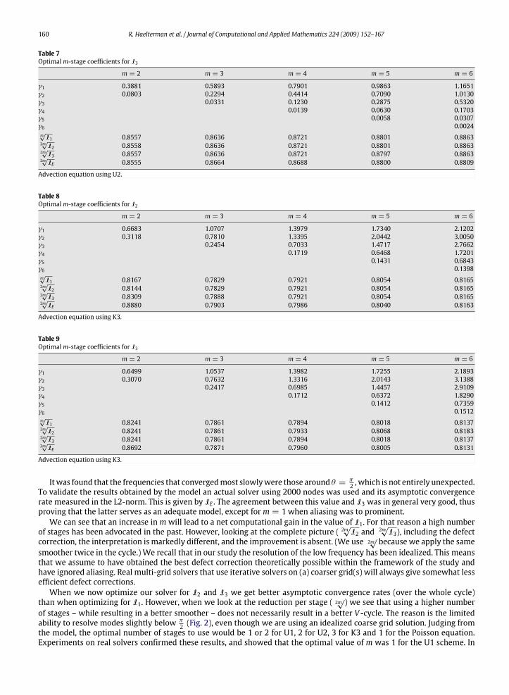
Table 7Optimalm-stage coefficients for I3

m = 2 m = 3 m = 4 m = 5 m = 6

γ1 0.3881 0.5893 0.7901 0.9863 1.1651γ2 0.0803 0.2294 0.4414 0.7090 1.0130γ3 0.0331 0.1230 0.2875 0.5320γ4 0.0139 0.0630 0.1703γ5 0.0058 0.0307γ6 0.0024m√

I1 0.8557 0.8636 0.8721 0.8801 0.88632m√

I2 0.8558 0.8636 0.8721 0.8801 0.88632m√

I3 0.8557 0.8636 0.8721 0.8797 0.88632m√

IE 0.8555 0.8664 0.8688 0.8800 0.8809

Advection equation using U2.

Table 8Optimalm-stage coefficients for I2

m = 2 m = 3 m = 4 m = 5 m = 6

γ1 0.6683 1.0707 1.3979 1.7340 2.1202γ2 0.3118 0.7810 1.3395 2.0442 3.0050γ3 0.2454 0.7033 1.4717 2.7662γ4 0.1719 0.6468 1.7201γ5 0.1431 0.6843γ6 0.1398m√

I1 0.8167 0.7829 0.7921 0.8054 0.81652m√

I2 0.8144 0.7829 0.7921 0.8054 0.81652m√

I3 0.8309 0.7888 0.7921 0.8054 0.81652m√

IE 0.8880 0.7903 0.7986 0.8040 0.8163

Advection equation using K3.

Table 9Optimalm-stage coefficients for I3

m = 2 m = 3 m = 4 m = 5 m = 6

γ1 0.6499 1.0537 1.3982 1.7255 2.1893γ2 0.3070 0.7632 1.3316 2.0143 3.1388γ3 0.2417 0.6985 1.4457 2.9109γ4 0.1712 0.6372 1.8290γ5 0.1412 0.7359γ6 0.1512m√

I1 0.8241 0.7861 0.7894 0.8018 0.81372m√

I2 0.8241 0.7861 0.7933 0.8068 0.81832m√

I3 0.8241 0.7861 0.7894 0.8018 0.81372m√

IE 0.8692 0.7871 0.7960 0.8005 0.8131

Advection equation using K3.

Itwas found that the frequencies that convergedmost slowlywere those around θ = π2 , which is not entirely unexpected.

To validate the results obtained by the model an actual solver using 2000 nodes was used and its asymptotic convergencerate measured in the L2-norm. This is given by IE . The agreement between this value and I3 was in general very good, thusproving that the latter serves as an adequate model, except form = 1 when aliasing was to prominent.We can see that an increase inm will lead to a net computational gain in the value of I1. For that reason a high number

of stages has been advocated in the past. However, looking at the complete picture ( 2m√

I2 and 2m√

I3), including the defectcorrection, the interpretation is markedly different, and the improvement is absent. (We use 2m

√ because we apply the samesmoother twice in the cycle.) We recall that in our study the resolution of the low frequency has been idealized. This meansthat we assume to have obtained the best defect correction theoretically possible within the framework of the study andhave ignored aliasing. Real multi-grid solvers that use iterative solvers on (a) coarser grid(s) will always give somewhat lessefficient defect corrections.When we now optimize our solver for I2 and I3 we get better asymptotic convergence rates (over the whole cycle)

than when optimizing for I1. However, when we look at the reduction per stage ( 2m√) we see that using a higher number

of stages – while resulting in a better smoother – does not necessarily result in a better V -cycle. The reason is the limitedability to resolve modes slightly below π

2 (Fig. 2), even though we are using an idealized coarse grid solution. Judging fromthe model, the optimal number of stages to use would be 1 or 2 for U1, 2 for U2, 3 for K3 and 1 for the Poisson equation.Experiments on real solvers confirmed these results, and showed that the optimal value of m was 1 for the U1 scheme. In

R. Haelterman et al. / Journal of Computational and Applied Mathematics 224 (2009) 152–167 161

Fig. 3. Optimal U1 scheme (m = 1; γ1 = 0.5). Figure left: Stability region and Fourier symbol. Figure right: Amplification curves |P ′m(λ(θ))| (dotted line)and |µV ,2(λ(θ))| (solid line).

Fig. 4. Optimal U2 scheme (m = 2; γ1 = 0.3881, γ2 = 0.0803). Figure left: Stability region and Fourier symbol. Figure right: Amplification curves|P ′m(λ(θ))| (dotted line) and |µV ,2(λ(θ))| (solid line).

general the experimental convergence rates again differed only within 0.5%–5% of the values of the theoretical model (basedon I3), except form = 1 in the U1 scheme, andm = 2 for the K3 scheme, which is believed to be due to the effect of aliasing(neglected in themodel). The integrated optimization approach (I3) yielded an improvement over the old coefficients,whichfor the optimal number of stages amounted to 33% for the K3 scheme (m = 3), 5% for the U2 (m = 2) scheme and equalperformance for U1 (m = 1). For higher values ofm the optimization of I3 steadily outperformed that of I1.We illustrate the results for the different optimal schemes by drawing the stability region S = {z ∈ C; |P ′m(z)| ≤

1} on which we superpose (−λ(θ)) and also give |P ′m(λ(θ))| (the amplification of the smoother) and |µV ,2(λ(θ))| (theamplification of the V -cycle). We point out that, due to rounding errors in the actual computation of Eq. (39), |µV ,2(λ(θ))|sometimes tended to 1 in the neighborhood of θ = 0 (see Figs. 3–5).It is clear that the new optimization procedure results in an amplification curve that respects the equal excursion

principle, but now taken over the complete V -cycle and that smoothing has been sacrificed to some extent.

6. Iterative scheme using a splitting of the discretization matrix

6.1. Formulation

In analogy to the Modified-Runge Kutta scheme [5] we propose a scheme that splits A in two parts

A = B+ C . (44)

162 R. Haelterman et al. / Journal of Computational and Applied Mathematics 224 (2009) 152–167

Fig. 5. Optimal K3 scheme (m = 3; γ1 = 1.0537, γ2 = 0.7632, γ3 = 0.2417). Figure left: Stability region and Fourier symbol. Figure right: Amplificationcurves |P ′m(λ(θ))| (dotted line) and |µV ,2(λ(θ))| (solid line).

The scheme is given by

U(o) = unV(o) = M−1r(o)U(1) = U(o) − γ1V(o)VB(1) = −M−1BV(o)VC (1) = −M−1CV(o)U(2) = U(1) − γB,2VB(1) − γC,2VC (1)VB(2) = −M−1BVB(1)VC (2) = −M−1CVC (1)...

VB(l) = −M−1BVB(l−1)VC (l) = −M−1CVC (l−1)U(l+1) = U(l) − γB,l+1VB(l) − γC,l+1VC (l)...

VB(m−1) = −M−1BVB(m−2)VC (m−1) = −M−1CVC (m−2)U(m) = U(m−1) − γB,mVB(m−1) − γC,mVC (m−1)un+1 = U(m)

(45)

which results in

en+1 = P ′′m(−M−1B,−M−1C)en (46)

where

P ′′m(z1, z2) = 1+

(γ1 +

m∑l=2

(γB,lz l−11 + γC,lz

l−12

))(z1 + z2). (47)

Again we note that it is not necessary to store intermediate results and that VB and VC can be computed in parallel.We limit ourselves to splittings where M−1B and M−1C have the same eigenvectors as M−1A, which is straightforward

if A results from a differencing scheme, as illustrated in Section 5. We number the eigenvalues λB,i and λC,i (i = 1, . . . , p) ofM−1B andM−1C respectively in such a way that

λB,i + λC,i = λi (i = 1, . . . , p). (48)

R. Haelterman et al. / Journal of Computational and Applied Mathematics 224 (2009) 152–167 163

Table 10Optimal coefficients for I3 when using the split scheme

U1 U2 K3

γ1 0.5000 0.2071 0.4580γB,2 0.0000 0.0000 0.0000γC,2 0.6043 0.1703 0.54714√

I3 0.6462 0.7779 0.62404√

IE 0.6413 0.7762 0.6391

Advection equation using different discretizations.

In this case, according to a well-known theorem in [10], (M−1B) and (M−1C) commute, which avoids problems with thecommutative property of the scalars in expression (47) and we can write

en+1i = P ′′m(−λB,i,−λC,i)eni . (49)

Wewill now propose splits such that λB is the real part and λC the imaginary part of λi. In other words where B = 12 (A+A

T)

and C = 12 (A− A

T).

6.1.1. Advection equation with U1We propose to split the differencing scheme (and hence A) as

1∆x

((−uj+1 + 2uj − uj−1

2

)+

(uj+1 − uj−1

2

))(50)

which will result in

λ(θ) =1∆x

(1− cos θ)︸ ︷︷ ︸λB(θ)

+1∆x

(i sin θ)︸ ︷︷ ︸λC (θ)

. (51)

This splitting is a very logical one as it writes the upwind discretization as the sum of a central discretization (imaginarypart) and a first order diffusion term (real part).

6.1.2. Advection equation with U2

( 12uj+2 − 2uj+1 + 3uj − 2uj−1 +

12uj−2

)+(−12uj+2 + 2uj+1 − 2uj−1 +

12uj−2

)2∆x

(52)

λ(θ) =12∆x

(3− 4 cos θ + cos(2θ))︸ ︷︷ ︸λB(θ)

+i2∆x

(4 sin θ − sin(2θ))︸ ︷︷ ︸λC (θ)

. (53)

Again the real part corresponds to a diffusion term, this time of third order.

6.1.3. Advection equation with K3

( 12uj+2 − 2uj+1 + 3uj − 2uj−1 +

12uj−2

)+(−12uj+2 + 4uj+1 − 4uj−1 +

12uj−2

)6∆x

(54)

λ(θ) =16∆x

(3− 4 cos θ + cos(2θ))︸ ︷︷ ︸λB(θ)

+i6∆x

(8 sin θ − sin(2θ))︸ ︷︷ ︸λC (θ)

. (55)

6.2. Results

The optimal coefficients obtained with this approach can be found in Table 10. It was found thatm = 2 gave the optimalefficiency for the three discretizations. Using more coefficients only improved the performance slightly but not enough tocompensate for the extra numerical work. It was also found that setting γB,2 (corresponding to the diffusive part) to zerodid not degrade performance too much. As this allowed us to reduce the number of coefficients (and hence matrix-vector

164 R. Haelterman et al. / Journal of Computational and Applied Mathematics 224 (2009) 152–167

Fig. 6. Figure left: stability region and Fourier symbol. Figure right: amplification curves |P ′′m(λ(θ))| (dotted line) and |µV ,2(λ(θ))| (solid line) for theoptimal split U1 scheme (m = 2; γ1 = 0.5000, γB,2 = 0.0000, γC,2 = 0.6043).

Fig. 7. Figure left: stability region and Fourier symbol. Figure right: amplification curves |P ′′m(λ(θ))| (dotted line) and |µV ,2(λ(θ))| (solid line) for theoptimal split U2 scheme (m = 2; γ1 = 0.2071, γB,2 = 0.0000, γC,2 = 0.1703).

multiplications) from 3 to 2 it was found that a higher efficiency was attained. The schemes were optimized for I3 andcompared with IE .Again, agreement between the theoretical model and the experimental results was very good. From the data it is clear

that this split approach withm = 2 and γB,2 = 0 can lead to improvements in the order of 10% for U1 and U2 and 20% for K3with respect to our optimal results in Section 5. We illustrate the results for the different optimal split schemes by drawingthe stability region S = {z ∈ C; |P ′′m(z)| ≤ 1} on which we superpose (−λ(θ)) and also give |P

′′m(λ(θ))| and |µV ,2(λ(θ))|

(see Figs. 6–8).

7. Advection–diffusion equation

Often a certain amount of artificial diffusion is added to the advection Eq. (20) to stabilize it when the advection term isdiscretized with a central discretization. If we choose a third order dissipative term this becomes

∂u∂t+ a

∂u∂x+ µ∆x3

∂4u∂x4= 0 (56)

where a, µ ∈ R+o . Again we are only interested in the steady-state solution and take a = 1 for the sake of simplicity.Discretization of the space operators gives

12∆x

(uj+1 − uj−1

)+µ

∆x

(uj+2 − 4uj+1 + 6uj − 4uj−1 + uj−2

). (57)

R. Haelterman et al. / Journal of Computational and Applied Mathematics 224 (2009) 152–167 165

Fig. 8. Figure left: stability region and Fourier symbol. Figure right: amplification curves |P ′′m(λ(θ))| (dotted line) and |µV ,2(λ(θ))| (solid line) for theoptimal split K3 scheme (m = 2; γ1 = 0.4580, γB,2 = 0.0000, γC,2 = 0.5471).

This is quite similar to the discretizations of the previous section with a natural splitting between the Hermitian (diffusive)and anti-Hermitian (convective) part.The resulting Fourier symbol is

λ(θ) =2µ∆x

(3− 4 cos θ + cos(2θ))︸ ︷︷ ︸λB(θ)

+i∆x

(sin θ)︸ ︷︷ ︸λC (θ)

. (58)

The iterative solution of this equation has been studied in [6,7,9], which led to the so called modified Runge–Kutta schemeand the Martinelli–Jameson coefficients, which were obtained by trial and error. Later Hosseini [5] analytically confirmedthe results of Martinelli and Jameson. The Modified Runge–Kutta scheme treats the convective and diffusive parts of theresidual differently. We use the formulation given in [8], adapting it to the conventions and notations used in this paper.

U(o) = un

U(1) = U(o) − α1h(r(o)C + r

(o)B

)...

U(l) = U(o) − αlh

(r(l−1)C +

l−1∑k=0

Γl,kr(k)B

)un+1 = U(m).

(59)

Here r(l)C stands for the convective, and r(l)B for the dissipative part of the residual at stage l and

Γl,k =

{βl if k = l− 1(1− βl)Γl−1,k if k 6= l− 1. (60)

The Martinelli–Jameson coefficients are given by:

α1 =14

β1 = 1

α2 =16

β2 = 0

α3 =38

β3 =1425

α4 =12

β4 = 0

α5 = 1 β5 =1125

and h = 3.93, µ = 1/32. The resulting stability region, Fourier symbol and amplification curves are given in Fig. 9.

166 R. Haelterman et al. / Journal of Computational and Applied Mathematics 224 (2009) 152–167

Fig. 9. Advection–diffusion equation with 5-stage Martinelli–Jameson coefficients and h = 3.8058. Figure left: stability region and Fourier symbol. Figureright: amplification curves |P ′′m(λ(θ))| (dotted line) and |µV ,2(λ(θ))| (solid line).

Fig. 10. Advection–diffusion equation with split scheme (m = 3; γ1 = 1.4226, γB,2 = 0, γC,2 = 1.2826, γB,3 = 0, γC,3 = 1.3000). Figure left: Stabilityregion and Fourier symbol. Figure right: Amplification curves |P ′′m(λ(θ))| (dotted line) and |µV ,2(λ(θ))| (solid line).

Testing our objective functions on this scheme, keeping the α and β coefficients andµ but optimizing h for I1 and I3 wefound

• I1 = 0.5831 for h = 3.8231• I3 = 0.3407 for h = 3.8058

which is not that different from the value found in [5]. We illustrate these results by drawing the stability regionS = {z ∈ C; |P ′′m(z)| ≤ 1} on which we superpose (−λ(θ)) and also give |P

′′m(λ(θ))| and |µV ,2(λ(θ))|. We only do this

for h = 3.8058 as both results are qualitatively similar.This scheme uses 5 stages, with 5 evaluations of the advective and 3 evaluations of the diffusive residual, which is quite

costly. We like to point out that the spike in the amplification curve around θ = π2 is due to the way we model the low

and high frequencies separately. It seems reasonable that a better model would smoothen this curve and that therefore theoptimal value of I3 will be slightly lower.We now try to find a split scheme, according to our own formulation in Section 6 for this equation, minimizing I3 and

using a low number of stages. It was found that a scheme with m = 3 gave the best result, keeping µ = 1/32. Setting γB,2and γB,3 to zero again did not degrade performance too much and offered a computational saving of 40%. With this in mindthe optimal scheme was given by (γ1, γB,2, γC,2, γB,3, γC,3) = (1.4226, 0, 1.2826, 0, 1.3000), which gave an optimal valueI3 = 0.1190 ( 3

√I3 = 0.4919), which only differed by less than 1% from values measured on the real solver.

We note that these values are substantially lower than the optimal values found for the Martinelli–Jameson scheme andeffectively use only 3 coefficients. We illustrate this schemes in Fig. 10.

R. Haelterman et al. / Journal of Computational and Applied Mathematics 224 (2009) 152–167 167

8. Conclusions

Previous studies [1,4,5,11], that optimized the Runge–Kutta parameters for the high frequency domain, showed that abetter smoother can be obtainedwhen using a high number of stages.While this is true, we discovered that for the complete2-grid cycle the gain from a higher number of stages does not outweigh the extra computational cost, due to the limitationsof the defect correction. It actually appears that using a low number of stages gives the best results. We optimized thecoefficients for a complete V -cycle and obtained improvements up to 20% for higher order discretizations (measured perstage). When we choose to treat the Hermitian part of the discretization separately from the anti-Hermitian part, furthergains could be obtained; these were of the order of 30%–50% using a low number of stages (measured per stage).We compared the latter with the Martinelli–Jameson scheme for the advection–diffusion equation and found an

asymptotic convergence rate that was 66% better (over a whole V -cycle) but using 3, instead of 8, matrix-vectormultiplications in the smoother.

References

[1] L.A. Catalano, H. Deconinck, Two-dimensional optimization of smoothing properties ofmulti-stage schemes applied to hyperbolic equations, TechnicalNote 173, Von Karman Institute for Fluid Dynamics, 1990.

[2] L.V. Fauset, Applied Numerical Analysis Using MATLAB, Prentice Hall, Upper Saddle River, NJ, 1999.[3] R. Haelterman, An analytical quantification of the optimization of multi-stage solvers, in: ICCAM 2006, Twelfth International Congress onComputational and Applied Mathematics, Leuven, Belgium, 10–14 July, 2006.

[4] K. Hosseini, J.J. Alonso, Practical implementation and improvement of preconditioning methods for explicit multistage flow solvers, AIAA 2004–0763,42nd AIAA Aerospace Meeting and Exhibit, Reno, NV, January 2004.

[5] K. Hosseini, Practical implementation of robust preconditioners for optimized multistage flow solvers, Ph.D. Thesis, Stanford University, 2005.[6] A. Jameson, Numerical solution of the Euler equations for compressible inviscid fluids, in: F. Angrand, A. Dervieux, J.A. Dé sidé ri, R. Glowinski (Eds.),Numerical Methods for the Euler Equations of Fluid Dynamics, SIAM, Philadelphia, 1985, pp. 199–245.

[7] A. Jameson, Analysis and design of numerical schemes for gas dynamics 1, artificial diffusion, upwind biasing, limiter and their effect on multigridconvergence, Int. J. Comp. Fluid Dyn. 4 (1995) 171–218.

[8] J.V. Lassaline, Optimal multistage relaxation coefficients for multigrid flow solvers, http://www.ryerson.ca/~jvl/papers/cfd2005.pdf.[9] L. Martinelli, Calculations of viscous flows with a multigrid method, Ph.D. Thesis, Princeton University, 1987.[10] R.S. Varga, Matrix Iterative Analysis, in: Springer Series in Computational Mathematics, vol. 27, Springer-Verlag, Berlin, 2000.[11] B. Van Leer, C.H. Tai, K.G. Powell, Design of optimally smoothing multi-stage schemes for the Euler equations, AIAA Paper 89–1923, 1989.[12] D.M. Young, Iterative Solution of Large Linear Systems, Dover Publications, New York, 1971.