He's variational iteration method for solving linear and non-linear systems of ordinary differential...

Applied Mathematics and Computation 191 (2007) 287–297

www.elsevier.com/locate/amc

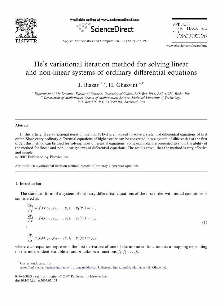
He’s variational iteration method for solving linearand non-linear systems of ordinary differential equations

J. Biazar a,*, H. Ghazvini a,b

a Department of Mathematics, Faculty of Sciences, University of Guilan, P.O. Box 1914, P.C. 41938, Rasht, Iranb Department of Mathematics, School of Mathematical Science, Shahrood University of Technology,

P.O. Box 316, P.C. 3619995161, Shahrood, Iran

Abstract

In this article, He’s variational iteration method (VIM) is employed to solve a system of differential equations of firstorder. Since every ordinary differential equations of higher order can be converted into a system of differential of the firstorder, this method can be used for solving most differential equations. Some examples are presented to show the ability ofthe method for linear and non-linear systems of differential equations. The results reveal that the method is very effectiveand simple.� 2007 Published by Elsevier Inc.

Keywords: He’s variational iteration method; System of ordinary differential equations

1. Introduction

The standard form of a system of ordinary differential equations of the first order with initial conditions isconsidered as

0096-3

doi:10.

* CoE-m

dy1

dx¼ f1ðx; y1; y2; . . . ; ynÞ; y1ðx0Þ ¼ y1;

dy2

dx¼ f2ðx; y1; y2; . . . ; ynÞ; y2ðx0Þ ¼ y2;

..

.

dyn

dx¼ fnðx; y1; y2; . . . ; ynÞ; ynðx0Þ ¼ yn;

ð1Þ

where each equation represents the first derivative of one of the unknown functions as a mapping dependingon the independent variable x, and n unknown functions f1; f2; . . . ; fn.

003/$ - see front matter � 2007 Published by Elsevier Inc.

1016/j.amc.2007.02.153

rresponding author.ail addresses: [email protected], [email protected] (J. Biazar), [email protected] (H. Ghazvini).

mailto:[email protected]



288 J. Biazar, H. Ghazvini / Applied Mathematics and Computation 191 (2007) 287–297

For many naturally occurring phenomena, the most appropriate form in which to express a differentialequation is as a higher order system. For example, an equation might be of the form

yðnÞ ¼ /ðx; y; y0; y00; . . . ; yðn�1ÞÞ; ð2Þ
with initial values given for yðx0Þ; y0ðx0Þ; y 00ðx0Þ; . . . ; yðn�1Þðx0Þ:
By identifying yðxÞ ¼ y1ðxÞ; y0ðxÞ ¼ y2ðxÞ; . . . ; yðn�1ÞðxÞ ¼ ynðxÞ, we can rewrite Eq. (2), the system in theform

dy1

dx¼ y2ðxÞ; y1ðx0Þ ¼ yðx0Þ;

dy2

dx¼ y3ðxÞ; y2ðx0Þ ¼ y0ðx0Þ;

..

.

dyn

dx¼ /ðx; y1; y2; . . . ; ynÞ; ynðx0Þ ¼ yðn�1Þðx0Þ;

ð3Þ

where is a system of differential equations of the first order.Since every ordinary differential equation of order n can be written as a system consisting of n ordinary

differential equation of order one, we restrict our study to the systems of differential equations of the firstorder.

2. He’s variational iteration method

The variational iteration method [1–9], which accurately is a modified general Lagrange multiplier method[10], has been shown to solve effectively, easily and accuracy, large class of nonlinear problems with approx-imations which convergen rapidly to accurate solution. To illustrate the method, let us consider the followingnonlinear equation:

LuðtÞ þ NuðtÞ ¼ gðtÞ; ð4Þ
where L is a linear operator, N is a nonlinear operator and gðtÞ is a known analytical function. According tothe variational iteration method, we can construct the following correction functional:
unþ1ðtÞ ¼ unðtÞ þZ t

0

kðnÞðLunðnÞ þ NunðnÞ � gðnÞÞdn; ð5Þ

where k is a general Lagrange multiplier which can be identified via variational theory, u0ðtÞ is an initialapproximation with possible unknowns, and ~un is considered as restricted variation [11], i.e. d~un ¼ 0.

3. Application

In this section, we present six examples. First, fifth and sixth examples are considered to illustrate themethod for linear and non-linear systems of ordinary differential equations of order one. While in the second,third and fourth examples we solve a differential equation of higher order by converting it into a system ofdifferential equations of the first order.

Example 1. Consider the following system of non-homogeneous differential equations:

dy1

dx¼ y3 � cos x; y1ð0Þ ¼ 1;

dy2

dx¼ y3 � ex; y2ð0Þ ¼ 0;

dy3

dx¼ y1 � y2; y3ð0Þ ¼ 2:

ð6Þ

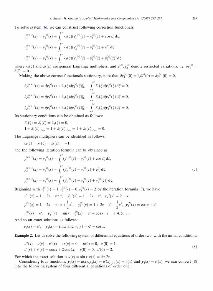
J. Biazar, H. Ghazvini / Applied Mathematics and Computation 191 (2007) 287–297 289

To solve system (6), we can construct following correction functionals:

yðnþ1Þ1 ðxÞ ¼ yðnÞ1 ðxÞ þ

Z x

0

k1ðnÞðy01ðnÞðnÞ � ~yðnÞ3 ðnÞ þ cos nÞdn;


Z x

0

k2ðnÞðy02ðnÞðnÞ � ~yðnÞ3 ðnÞ þ enÞdn;


Z x

0

k3ðnÞðy03ðnÞðnÞ � ~yðnÞ1 ðnÞ þ ~yðnÞ2 ðnÞÞdn:

where k1ðnÞ and k2ðnÞ are general Lagrange multipliers, and ~yðnÞ1 ; ~yðnÞ2 denote restricted variations, i.e. d~yðnÞ1 ¼d~yðnÞ2 ¼ 0:

Making the above correct functionals stationary, note that dyðnÞ1 ð0Þ ¼ dyðnÞ2 ð0Þ ¼ dyðnÞ3 ð0Þ ¼ 0;

dyðnþ1Þ1 ðxÞ ¼ dyðnÞ1 ðxÞ þ k1ðnÞdyðnÞ1 ðnÞj

x0 �

Z x

0

k01ðnÞdyðnÞ1 ðnÞdn ¼ 0;


x0 �

Z x

0



x0 �

Z x

0


Its stationary conditions can be obtained as follows:

k01ðnÞ ¼ k02ðnÞ ¼ k03ðnÞ ¼ 0;

1þ k1ðnÞjn¼x ¼ 1þ k2ðnÞjn¼x ¼ 1þ k3ðnÞjn¼x ¼ 0:

The Lagrange multipliers can be identified as follows:

k1ðnÞ ¼ k2ðnÞ ¼ k3ðnÞ ¼ �1:

and the following iteration formula can be obtained as

yðnþ1Þ1 ðxÞ ¼ yðnÞ1 ðxÞ �

Z x

0

ðy01ðnÞðnÞ � yðnÞ3 ðnÞ þ cos nÞdn;


Z x

0

ðy02ðnÞðnÞ � yðnÞ3 ðnÞ þ enÞdn;


Z x

0

ðy03ðnÞðnÞ � yðnÞ1 ðnÞ þ yðnÞ2 ðnÞÞdn:

ð7Þ

Beginning with yð0Þ1 ðxÞ ¼ 1; yð0Þ2 ðxÞ ¼ 0; yð0Þ3 ðxÞ ¼ 2 by the iteration formula (7), we have

yð1Þ1 ðxÞ ¼ 1þ 2x� sin x; yð1Þ2 ðxÞ ¼ 1þ 2x� ex; yð1Þ3 ðxÞ ¼ 2þ x;

yð2Þ1 ðxÞ ¼ 1þ 2x� sin xþ 1

2x2; yð2Þ2 ðxÞ ¼ 1þ 2x� ex þ 1

2x2; yð2Þ3 ðxÞ ¼ cos xþ ex;

yðiÞ1 ðxÞ ¼ ex; yðiÞ2 ðxÞ ¼ sin x; yðiÞ3 ðxÞ ¼ ex þ cos x; i ¼ 3; 4; 5; . . . :

And so an exact solutions as follows:

y1ðxÞ ¼ ex; y2ðxÞ ¼ sin x and y3ðxÞ ¼ ex þ cos x:

Example 2. Let us solve the following system of differential equations of order two, with the initial conditions:

u00ðxÞ þ uðxÞ � v00ðxÞ � 4vðxÞ ¼ 0; uð0Þ ¼ 0; u0ð0Þ ¼ 1;

u0ðxÞ þ v0ðxÞ ¼ cos xþ 2 cos 2x; vð0Þ ¼ 0; v0ð0Þ ¼ 2:ð8Þ

For which the exact solution is uðxÞ ¼ sin x; vðxÞ ¼ sin 2x:Considering four functions, y1ðxÞ ¼ uðxÞ; y2ðxÞ ¼ u0ðxÞ; y1ðxÞ ¼ uðxÞ and y4ðxÞ ¼ v0ðxÞ; we can convert (8)

into the following system of four differential equations of order one:

TableNume

xi

00.10.20.30.40.50.60.70.80.91


y01ðxÞ ¼ y2ðxÞ; y1ð0Þ ¼ 0;

y02ðxÞ ¼ �1

2y1ðxÞ þ 2y3ðxÞ �

1

2ðsin xþ 4 sin 2xÞ; y2ð0Þ ¼ 1;

y03ðxÞ ¼ y4ðxÞ; y3ð0Þ ¼ 0;

y04ðxÞ ¼1

2y1ðxÞ � 2y3ðxÞ �

1

2ðsin xþ 4 sin 2xÞ; y4ð0Þ ¼ 2:

Following the discussion presented in Example 1, we obtain the recurrence relation:


Z x

0

ðy01ðnÞðnÞ � yðnÞ2 ðnÞÞdn; yð0Þ1 ðxÞ ¼ 0;


Z x

0

ðy02ðnÞðnÞ þ 1

2yðnÞ1 ðnÞ � 2yðnÞ3 ðnÞ þ

1

2ðsin nþ 4 sin 2nÞÞdn; yð0Þ2 ðxÞ ¼ 1;


Z x

0

ðy03ðnÞðnÞ � yðnÞ4 ðnÞÞdn; yð0Þ3 ðxÞ ¼ 0;


Z x

0

ðy04ðnÞðnÞ � 1

2yðnÞ1 ðnÞ þ 2yðnÞ3 ðnÞ þ

1

2ðsin nþ 4 sin 2nÞÞdn; yð0Þ4 ðxÞ ¼ 2:

After 15 iterative the approximate solutions as follows:

uðxÞ � yð15Þ1 ðxÞ ¼ 122:011x� 121:070 sin xþ 0:0298 sin 2x� 20:305x3 þ 1:009x5 � 0:0235x7

þ 0:000294x9 � 0:15310�5x11 � 0:19610�7x13 þ 0:65310�9x15;

vðxÞ � yð15Þ3 ðxÞ ¼ �122:011xþ 122:070 sin xþ 0:970 sin 2xþ 20:305x3 � 1:009x5 þ 0:0235x7

� 0:000294x9 þ 0:15310�5x11 þ 0:19610�7x13 � 0:65310�9x15:

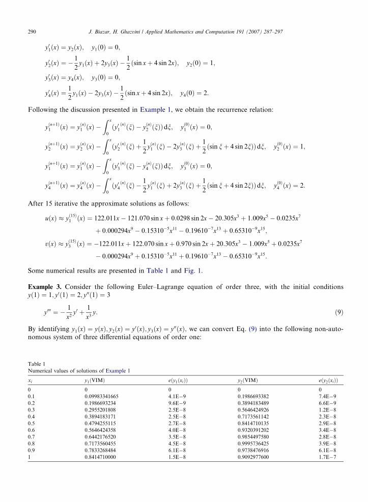
Some numerical results are presented in Table 1 and Fig. 1.

Example 3. Consider the following Euler–Lagrange equation of order three, with the initial conditionsyð1Þ ¼ 1; y0ð1Þ ¼ 2; y 00ð1Þ ¼ 3

y 000 ¼ � 1

x2y0 þ 1

x3y: ð9Þ

By identifying y1ðxÞ ¼ yðxÞ; y2ðxÞ ¼ y0ðxÞ; y3ðxÞ ¼ y00ðxÞ; we can convert Eq. (9) into the following non-auto-nomous system of three differential equations of order one:

1rical values of solutions of Example 1

y1ðVIMÞ eðy1ðxiÞÞ y2ðVIMÞ eðy2ðxiÞÞ0 0 0 00.09983341665 4.1E�9 0.1986693382 7.4E�90.1986693234 9.6E�9 0.3894183489 6.6E�90.2955201808 2.5E�8 0.5646424926 1.2E�80.3894183171 2.5E�8 0.7173561142 2.3E�80.4794255115 2.7E�8 0.8414710135 2.9E�80.5646424358 4.0E�8 0.9320391202 3.4E�80.6442176520 3.5E�8 0.9854497580 2.8E�80.7173560455 4.5E�8 0.9995736425 3.9E�80.7833268484 6.1E�8 0.9738476916 6.1E�80.8414710000 1.5E�8 0.9092977600 1.7E�7

Fig. 1. The plots of approximation and exact solutions of Example 2.


dy1

dx¼ y2; y1ð1Þ ¼ 1;

dy2

dx¼ y3; y2ð1Þ ¼ 2;

dy3

dx¼ � 1

x2y2 þ

1

x3y1; y3ð1Þ ¼ 3:

We can construct the following correction functionals:


Z x

1

k1ðnÞðy01ðnÞðnÞ � ~yðnÞ2 ðnÞÞdn;


Z x

1



Z x

1

k3ðnÞðy03ðnÞðnÞ þ 1

n2~yðnÞ2 ðnÞ �

1

n3~yðnÞ1 ðnÞÞdn;


k01ðnÞ ¼ k02ðnÞ ¼ k03ðnÞ ¼ 0;

1þ k1ðnÞjn¼x ¼ 1þ k2ðnÞjn¼x ¼ 1þ k3ðnÞjn¼x ¼ 0:

The Lagrange multipliers can be identified as follows:

k1ðnÞ ¼ k2ðnÞ ¼ k3ðnÞ ¼ �1:

He’s variational iteration method consists of the following scheme:


Z x

1

ðy01ðnÞðnÞ � yðnÞ2 ðnÞÞdn;


Z x

1



Z x

1

ðy03ðnÞðnÞ þ 1

n2yðnÞ2 ðnÞ �

1

n3yðnÞ1 ðnÞÞdn;

ð10Þ

Starting with initial approximations yð0Þ1 ðxÞ ¼ 1; yð0Þ2 ðxÞ ¼ 2; yð0Þ3 ðxÞ ¼ 3; from (10), we can obtain followingresults:

y11ðxÞ ¼ �1þ 2x;

y21ðxÞ ¼

1

2� xþ 3

2x2;

TableNume

xi

00.10.20.30.40.50.60.70.80.91


y31ðxÞ ¼

9

4þ 2ðln x� 1Þxþ 3

4x2 þ 1

2ln x;

y41ðxÞ ¼ �1� 3ð1þ ln xÞxþ ð5� 3

2ln xÞx2 � 1

2ln x;

y51ðxÞ ¼ xð1þ ln xþ ðln xÞ2Þ:

After five steps the exact solutions as follows:

yðxÞ ¼ xð1þ ln xþ ðln xÞ2Þ:

Example 4. Consider the following non-linear ordinary differential equation of order two, with the initial con-ditions yð0Þ ¼ �1; y0ð0Þ ¼ 0;

y 002 � 2y 00 � 2xy 0 þ y 02 þ x2 ¼ 0: ð11Þ
For which the exact solution is yðxÞ ¼ 1
2x2 � cos x:

Considering the two functions, y1ðxÞ ¼ yðxÞ; y2ðxÞ ¼ y0ðxÞ; we can convert (11) into the following non-linearsystem of two differential equations of order one:

dy1

dx¼ y2ðxÞ; y1ð0Þ ¼ �1;

dy2

dx¼ 1þ

ffiffiffiffiffiffiffiffiffiffiffiffiffiffiffiffiffiffiffiffiffiffiffiffiffiffiffiffiffiffiffiffi1� ðy2ðxÞ � xÞ2

q; y2ð0Þ ¼ 0:

Its correction functionals can be easily constructed.


Z x

0



Z x

0

k2ðnÞðy02ðnÞðnÞ � 1�

ffiffiffiffiffiffiffiffiffiffiffiffiffiffiffiffiffiffiffiffiffiffiffiffiffiffiffiffiffiffiffiffiffiffiffi1� ð~yðnÞ2 ðnÞ � nÞ2

qÞdn:

The Lagrange multipliers can be identified as k1ðnÞ ¼ �1; k2ðnÞ ¼ �1 and the following iteration formula canbe obtained as


Z x

0



Z x

0

ðy02ðnÞðnÞ � 1�

ffiffiffiffiffiffiffiffiffiffiffiffiffiffiffiffiffiffiffiffiffiffiffiffiffiffiffiffiffiffiffiffiffiffiffi1� ðyðnÞ2 ðnÞ � nÞ2

qÞdn:

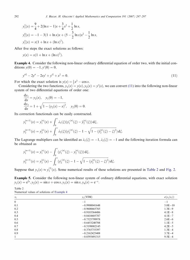
Suppose that y1ðxÞ � yð3Þ1 ðxÞ. Some numerical results of these solutions are presented in Table 2 and Fig. 2.

Example 5. Consider the following non-linear system of ordinary differential equations, with exact solutiony1ðxÞ ¼ e2x; y2ðxÞ ¼ sin xþ cos x; y3ðxÞ ¼ sin x; y4ðxÞ ¼ e�x:

2rical values of solutions of Example 4

y1ðVIMÞ eðy1ðxiÞÞ�1 �1�0.9900041648 5.0E�10�0.9600665765 1.3E�9�0.9103364486 4.1E�8�0.8410605787 4.1E�7�0.7525799978 2.6E�6�0.6453240708 1.1E�5�0.5198002145 4.2E�5�0.3765755397 1.3E�4�0.2162425408 3.7E�4�0.0393491315 9.5E�4

Fig. 2. The plot of approximation and exact solutions of Example 4.


dy1

dx¼ 2e4xy2

4;

dy2

dx¼ y1 � y3 þ cos x� e2x;

dy3

dx¼ y2 � y4 þ e�x � sin x;

dy4

dx¼ �e�5xy2

1:

We can construct following correction functionals as follows:


Z x

0

k1ðnÞðy01ðnÞðnÞ � 2e4nð~yðnÞ4 ðnÞÞ

2Þdn;


Z x

0

k2ðnÞðy02ðnÞðnÞ � ~yðnÞ1 ðnÞ þ ~yðnÞ3 ðnÞ � cos nþ e2nÞdn;


Z x

0

k3ðnÞðy03ðnÞðnÞ � ~yðnÞ2 ðnÞ þ ~yðnÞ4 ðnÞ � e�n þ sin nÞdn;


Z x

0

k4ðnÞðy04ðnÞðnÞ þ e�5nð~yðnÞ1 ðnÞÞ

2Þdn:

Making the above correction functionals stationary, we can obtain following stationary conditions:

k01ðnÞ ¼ k02ðnÞ ¼ k03ðnÞ ¼ k04ðnÞ ¼ 0;

1þ k1ðnÞjn¼x ¼ 1þ k2ðnÞjn¼x ¼ 1þ k3ðnÞjn¼x ¼ 1þ k4ðnÞjn¼x ¼ 0:

The Lagrange multipliers, therefore, can be easily identified as

k1ðnÞ ¼ k2ðnÞ ¼ k3ðnÞ ¼ k4ðnÞ ¼ �1:

Therefore, the iteration formula can be expressed


Z x

0

ðy01ðnÞðnÞ � 2e4nð~yðnÞ4 ðnÞÞ

2Þdn;


Z x

0

ðy02ðnÞðnÞ � ~yðnÞ1 ðnÞ þ ~yðnÞ3 ðnÞ � cos nþ e2nÞdn;


Z x

0

ðy03ðnÞðnÞ � ~yðnÞ2 ðnÞ þ ~yðnÞ4 ðnÞ � e�n þ sin nÞdn;


Z x

0

ðy04ðnÞðnÞ þ e�5nð~yðnÞ1 ðnÞÞ

2Þdn:


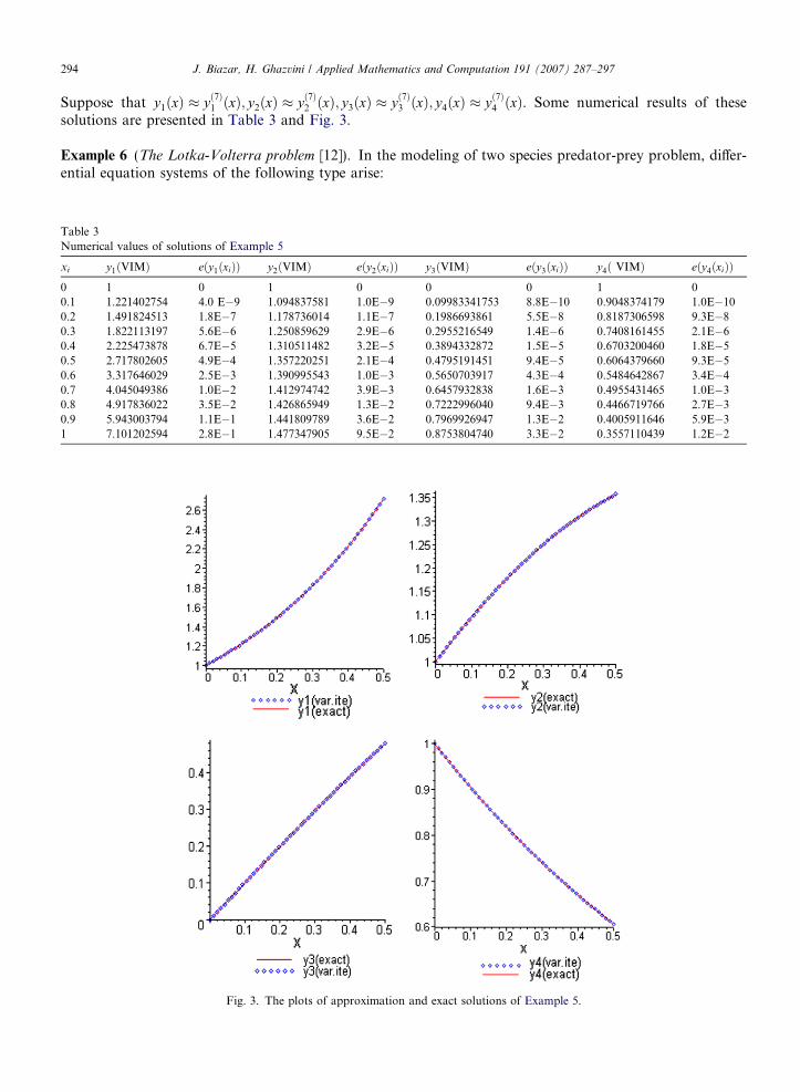
Suppose that y1ðxÞ � yð7Þ1 ðxÞ; y2ðxÞ � yð7Þ2 ðxÞ; y3ðxÞ � yð7Þ3 ðxÞ; y4ðxÞ � yð7Þ4 ðxÞ. Some numerical results of thesesolutions are presented in Table 3 and Fig. 3.

Example 6 (The Lotka-Volterra problem [12]). In the modeling of two species predator-prey problem, differ-ential equation systems of the following type arise:

Table 3Numerical values of solutions of Example 5

xi y1ðVIMÞ eðy1ðxiÞÞ y2ðVIMÞ eðy2ðxiÞÞ y3ðVIMÞ eðy3ðxiÞÞ y4ð VIMÞ eðy4ðxiÞÞ0 1 0 1 0 0 0 1 00.1 1.221402754 4.0 E�9 1.094837581 1.0E�9 0.09983341753 8.8E�10 0.9048374179 1.0E�100.2 1.491824513 1.8E�7 1.178736014 1.1E�7 0.1986693861 5.5E�8 0.8187306598 9.3E�80.3 1.822113197 5.6E�6 1.250859629 2.9E�6 0.2955216549 1.4E�6 0.7408161455 2.1E�60.4 2.225473878 6.7E�5 1.310511482 3.2E�5 0.3894332872 1.5E�5 0.6703200460 1.8E�50.5 2.717802605 4.9E�4 1.357220251 2.1E�4 0.4795191451 9.4E�5 0.6064379660 9.3E�50.6 3.317646029 2.5E�3 1.390995543 1.0E�3 0.5650703917 4.3E�4 0.5484642867 3.4E�40.7 4.045049386 1.0E�2 1.412974742 3.9E�3 0.6457932838 1.6E�3 0.4955431465 1.0E�30.8 4.917836022 3.5E�2 1.426865949 1.3E�2 0.7222996040 9.4E�3 0.4466719766 2.7E�30.9 5.943003794 1.1E�1 1.441809789 3.6E�2 0.7969926947 1.3E�2 0.4005911646 5.9E�31 7.101202594 2.8E�1 1.477347905 9.5E�2 0.8753804740 3.3E�2 0.3557110439 1.2E�2

Fig. 3. The plots of approximation and exact solutions of Example 5.


dudt¼ uð2� vÞ; uðt ¼ 0Þ ¼ a;

dvdt¼ vðu� 1Þ; vðt ¼ 0Þ ¼ b;

where the factors 2� v and u � 1 can be generalized in various ways. The two variables represent the time-dependent populations of which v is the population of predators, say foxes at time t, which feed on prey whosepopulation is denoted by u, say rabbits. It is assumed that u would have been able to grow exponentially with-out limit, if the predator had not been present, and that factor 2� v represents the modification to its growthrate because of harvesting by the predator.

For solving this system by He’s variational iteration method, we construct following correction functionals:

unþ1ðtÞ ¼ unðtÞ þZ t

ak1ðnÞðu0nðnÞ � 2unðnÞ þ ~unðnÞ~vnðnÞÞdn;

vnþ1ðtÞ ¼ vnðtÞ þZ t

bk2ðnÞðv0nðnÞ � ~unðnÞ~vnðnÞ þ vnðnÞÞdn:


k01ðnÞ þ 2k1ðnÞ ¼ 0;

1þ k1ðnÞjn¼t ¼ 0

and

k02ðnÞ � k2ðnÞ ¼ 0;

1þ k2ðnÞjn¼t ¼ 0:

The Lagrange multipliers, therefore, can be readily identified as

k1ðnÞ ¼ e�2ðn�tÞ and k2ðnÞ ¼ en�t:

The iteration formula can be expressed as

unþ1ðtÞ ¼ unðtÞ �Z t

ae�2ðn�tÞðu0nðnÞ � 2unðnÞ þ unðnÞvnðnÞÞdn;

vnþ1ðtÞ ¼ vnðtÞ �Z t

ben�tðv0nðnÞ � unðnÞvnðnÞ þ vnðnÞÞdn:

We start with initial approximations u0ðtÞ ¼ a; v0ðtÞ ¼ b: By the above iteration formula we can obtain the fol-lowing results:

u1ðtÞ ¼ a½ð1� 0:5bÞe2t þ 0:5b�;v1ðtÞ ¼ b½ð1� aÞe�t þ a�;u2ðtÞ ¼ a½ð1� b� 0:5833ab2 þ abþ 0:3333b2 � abt þ 0:5ab2tÞe2t

þ ðb� ab� 0:5b2 þ 0:5ab2Þet þ ð0:1667b2 � 0:1667ab2Þe�t þ 0:25ab2�;v2ðtÞ ¼ b½ð1� 0:5a� 0:5833a2bþ 0:1667a2 þ 0:25abþ 0:5abt � 0:5a2btÞe�t

þ ð0:3333a2 � 0:1667ab2Þe2t þ ð0:5a� 0:5a2 � 0:25abþ 0:25a2bÞet þ 0:5a2b�;

..

.

Two steps approximations to the solutions are considered uðtÞ � u2ðtÞ; vðtÞ � v2ðtÞ:


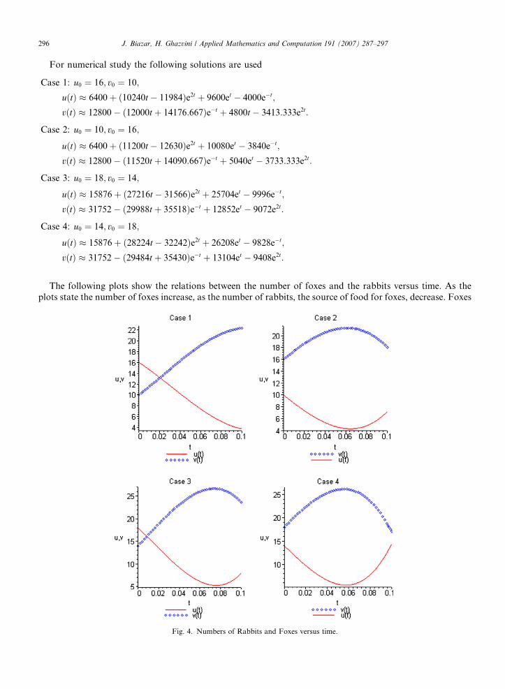
For numerical study the following solutions are used

Case 1: u0 ¼ 16; v0 ¼ 10;

uðtÞ � 6400þ ð10240t � 11984Þe2t þ 9600et � 4000e�t;

vðtÞ � 12800� ð12000t þ 14176:667Þe�t þ 4800t � 3413:333e2t:

Case 2: u0 ¼ 10; v0 ¼ 16;


vðtÞ � 12800� ð11520t þ 14090:667Þe�t þ 5040et � 3733:333e2t:

Case 3: u0 ¼ 18; v0 ¼ 14;


vðtÞ � 31752� ð29988t þ 35518Þe�t þ 12852et � 9072e2t:

Case 4: u0 ¼ 14; v0 ¼ 18;


vðtÞ � 31752� ð29484t þ 35430Þe�t þ 13104et � 9408e2t:

The following plots show the relations between the number of foxes and the rabbits versus time. As theplots state the number of foxes increase, as the number of rabbits, the source of food for foxes, decrease. Foxes

Fig. 4. Numbers of Rabbits and Foxes versus time.


will reach their maximum as the rabbits reach their minimum. Since the number of rabbits has decreased, thereis not enough food for foxes, so their number would decrease, and so on Fig. 4.

4. Conclusions

In this paper, He’s variational iteration method was used for finding the solutions for linear and nonlinearsystems of ordinary differential equations of the first order. In examples one and two, we derived the exactsolutions. For nonlinear systems, we usually derive very good approximations to the solutions, as in examplefour and five. It can be concluded that He’s variational iteration method is very powerful and efficient tech-nique in finding exact solutions for wide classes of problems.

The computations associated with the examples in this paper were performed using Maple 10.

References

[1] J.H. He, A new approach to nonlinear partial differential equations, Commun. Nonlinear Sci. Numer. Simul. 2 (4) (1997) 230–235.[2] J.H. He, Variational iteration method for delay differential equations, Commun. Nonlinear Sci. Numer. Simul. 2 (4) (1997) 235–236.[3] J.H. He, Approximate solution of nonlinear differential equations with convolution product nonlinearities, Comput. Meth. Appl.

Mech. Eng. 167 (1998) 69–73.[4] J.H. He, Variational iteration method-a kind of non-linear analytical technique some examples, Int. J. Nonlinear Mech. 34 (4) (1999)

699–708.[5] J.H. He, Approximate analytical solution for seepage flow with fractional derivatives in porous media, Comput. Meth. Appl. Mech.

Eng. 167 (1–2) (1998) 57–68.[6] J.H. He, Approximate solution of nonlinear differential equations with convolution product nonlinearities, Comput. Meth. Appl.

Mech. Eng. 167 (1–2) (1998) 69–73.[7] J.H. He, X.H. Wu, Construction of solitary solution and compaction-like solution by variational iteration method, Chaos Soliton.

Fract. 29 (1) (2006) 108–113.[8] J.H. He, Some asymptotic methods for strongly nonlinear equations, Int. J. Mod. Phys. B 20 (10) (2006) 1141–1199.[9] J.H. He, Variational iteration method for autonomous ordinary differential systems, Appl. Math. Comput. 114 (2–3) (2000) 115–123.

[10] M. Inokuti et al., General use of the Lagrange multiplier in nonlinear mathematical physics, in: S. Nemat Nasser (Ed.), VariationalMethod in the Mechanics of Solids, Pergamon Press, 1978, pp. 156–162.

[11] B.A. Finlayson, The Method of Weighted Residuals and Variational Principles, Academic Press, 1972.[12] J.C. Butcher, Numerical Methods for Ordinary Differential Equations, John Wiley & Sons, 2003.

He's variational iteration method for solving linear and non-linear systems of ordinary differential...

Documents

Transcript of He's variational iteration method for solving linear and non-linear systems of ordinary differential...