Solving Linear Ordinary Differential Equations using Singly Diagonally Implicit Runge-Kutta fifth...

Solving Linear Ordinary Differential Equations using Singly Diagonally Implicit Runge-Kutta fifth

order five-stage method

1 FUDZIAH ISMAIL, 1NUR IZZATI CHE JAWIAS,

1MOHAMED SULEIMAN AND

AZMI JAAFAR 2

1 Department of Mathematics, Faculty of Science

2 Department of Information System, Faculty of Computer Science and Information Technology

University Putra Malaysia 43400, Serdang, Selangor

MALAYSIA [email protected]

Abstract: - We constructed a new fifth order five-stage singly diagonally implicit Runge-Kutta (DIRK) method which is specially designed for the integrations of linear ordinary differential equations (LODEs). The restriction to linear ordinary differential equations (ODEs) reduces the number of conditions which the coefficients of the Runge-Kutta method must satisfy. The best strategy for practical purposes would be to choose the coefficients of the Runge-Kutta methods such that the error norm is minimized. Thus, here the error norm obtained from the error equations of the sixth order method is minimized so that the free parameters chosen are obtained from the minimized error norm. The stability aspect of the method is also looked into and found to have substantial region of stability, thus it is stable. Then a set of test problems are used to validate the method. Numerical results show that the new method is more efficient in terms of accuracy compared to the existing method.

Key-Words: - Runge-Kutta, Linear ordinary differential equations, Error norm.

1 Introduction Many algorithms have been proposed for the numerical solution of initial value problem

, ),( yxfy 00 )( yxy , (1) mf :

Such algorithm is the Singly Diagonally Implicit Runge-Kutta (SDIRK) method which was introduced to overcome some of the limitations of fully implicit and explicit Runge-Kutta method. Preliminary experiments have shown that these methods are usually more efficient than the standard Singly Implicit Runge-Kutta (SIRK) method and in many cases are competitive with backward differentiation formula. This algorithms can be used by both linear and nonlinear systems of ordinary equations.

However in this paper, we consider the numerical integration of linear inhomogeneous

systems of ordinary differential equations (ODEs) of the form

)(xGAyy (2) where A is a square matrix whose entries does not depend on or y x , and and are vectors. Such systems arise in the numerical solution of partial differential equations (PDEs) governing wave and heat phenomena after application of a spatial discretization such as finite-difference method. This type of partial differential equations can be solved numerically using methods suggested by Rasulov and Kul [7], Rasulov et. al [8] and Zabala and Ramos [12].

y )(xG

Actually there have been several attempts to develop efficient methods for integrating linear systems of ODEs. The basic concept of this method is that the major cost in evaluating the derivative function is in forming the matrix A and vector . )(xG

WSEAS TRANSACTIONS on MATHEMATICS Fudziah Ismail, Nur Izzati Che Jawias, Mohamed Suleiman, Azmi Jaafar

ISSN: 1109-2769 393 Issue 8, Volume 8, August 2009

Explicit Runge-Kutta method is very popular for simulations of wave equations; see Zingg and Chisholm [13], due to their high accuracy and low memory requirements.

To derive Runge-Kutta (RK) methods, we need to fulfill certain order equations; see Dormand [4]. These order equations resulted from the derivatives of the function ),( yxfy itself. If the function is linear then some of the error equations resulted by the nonlinearity in the derivative function can be removed, thus less order equations need to be satisfied, hence a more efficient method in some respect than the classical method can be derived. In this paper, we construct diagonally implicit Runge-Kutta method specifically for linear ODEs with constant coefficients. We consider the principal terms of the local truncation error to minimize the error norm. Then, a few test equations are used to validate the new method. 2 Materials and Methods

2.1 Derivation of the method In this section, we consider the following scalar ODE (2) ),( yxfy When a general s-stage diagonally implicit Runge-Kutta method is applied to the ODE, the following equations are obtained,

s

iiinn kbhyy

11 (3)

where

i

jjijnini kahyhcxfk

1),( (4)

We shall always assume that the row-sum

condition holds where i .

According to Dormand [3], there are 17 order equations (error equations) needed to be satisfied by the fifth order five-stage RK method. The restriction to linear ODEs reduces the number of equations which the coefficients of the RK method must satisfy see Zingg and

Chisholm [13]. The order equations are eliminated by exploiting the fact that, for linear ODEs,

,1

s

jiji ac

02

2

2

xyf

xf .

Zingg and Chisholm [13] too have derived a new explicit RK methods which are suitable for linear ODEs that are more efficient than the conventional RK methods.

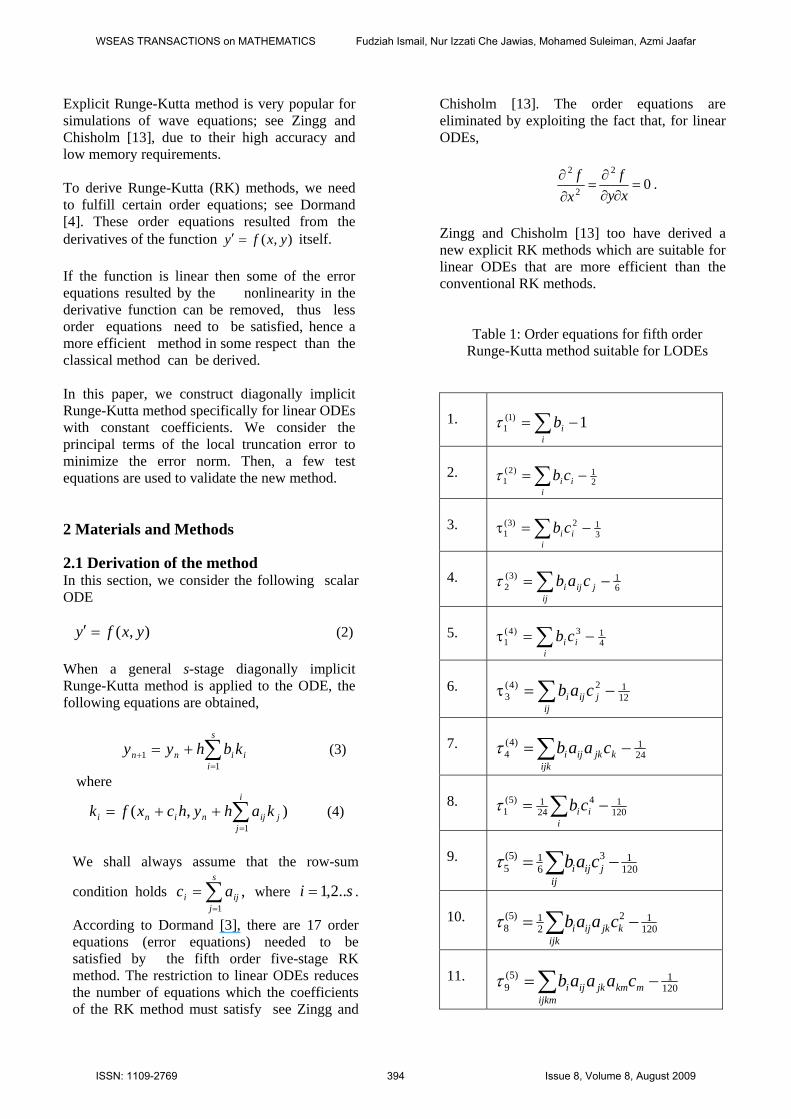
Table 1: Order equations for fifth order Runge-Kutta method suitable for LODEs

1.

i

ib 1)1(1

2.

iiicb 2

1)2(1

3.

iiicb 3

12)3(1

4.

ij

jiji cab 61)3(

2

5.

i

ii cb 413)4(

1

6.

ij

jiji cab 1212)4(

3

7.

ijk

kjkiji caab 241)4(

4

8.

i

iicb 12014

241)5(

1

9.

ij

jiji cab 12013

61)5(

5

10.

ijk

kjkiji caab 12012

21)5(

8

11.

ijkm

mkmjkiji caaab 1201)5(

9

s..2,1



https://www.researchgate.net/publication/220393765_Modern_Numerical_Methods_for_Ordinary_Differential_Equations?el=1_x_8&enrichId=rgreq-64f287bf667b6ba9135680378b0d6394-XXX&enrichSource=Y292ZXJQYWdlOzI0MjE0Mzg3NztBUzoyNzI1ODc5OTMzODI5NDJAMTQ0MjAwMTQ1MDY5OQ==

Using the simplifying assumption:

),1( jjiji cbab (5) 5,...,2j

We have ij

jiji cab 61 ( )2

1

iiicb )( 3

12 i

iicb ,

thus equation 4 can be removed, similarly we can remove equations 6 and 9 in table 1. Thus, using (5) the order equations are replaced by simpler equations. They are:

15

)1(4

)1(3

)1(2

5

44545

33535434

22525424323

cj

cbabj

cbababj

cbabababj

Altogether there are 11 equations needed to be satisfied and we have 15 unknowns. So, we can have four free parameters which are chosen to be and 432 ,, ccc . Solving which, we have all equations in terms of and 432 ,, ccc .

The order equations for the sixth order method are the 11 order equations in table 1 and the additional order equations given in table 2.2 as obtained by Zingg and Chisholm [13] .

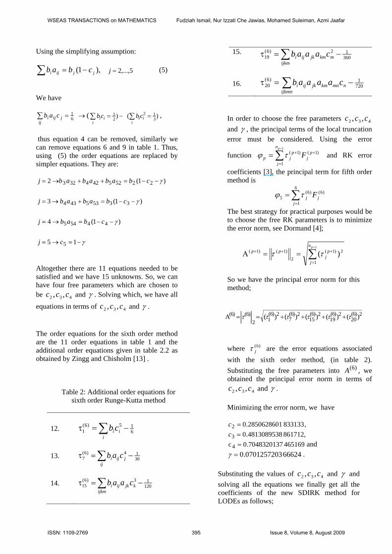
Table 2: Additional order equations for sixth order Runge-Kutta method

12.

i

iicb 615)6(

1

13.

ij

jiji cab 3014)6(

7

14.

ijkm

kjkiji caab 12013)6(

15

15.

ijkmmkmjkiji caaab 360

12)6(19

16.

ijkmn

nmnkmjkiji caaaab 7201)6(

20

In order to choose the free parameters and

432 ,, ccc , the principal terms of the local truncation

error must be considered. Using the error

function and RK error

coefficients [3], the principal term for fifth order method is

1

1

)1()1(pn

j

pj

pjp F

6

1

)6()6(5

jjj F

The best strategy for practical purposes would be to choose the free RK parameters is to minimize the error norm, see Dormand [4];

1

1

2)1(

2

)1()1( )(pn

j

pj

pp

So we have the principal error norm for this method;

2)6(

202)6(

192)6(

152)6(

72)6(

12)6()6( )()()()()(

where are the error equations associated with the sixth order method, (in table 2). Substituting the free parameters into , we obtained the principal error norm in terms of

and

)6(j

4c

)6(A

32 ,,cc .

Minimizing the error norm, we have

,8331332850628601.02 c861712,4813089538.03 c 4651697048320137.0c4 and 666240701257203.0 .

Substituting the values of and 432 ,, ccc and solving all the equations we finally get all the coefficients of the new SDIRK method for LODEs as follows;



https://www.researchgate.net/publication/220393765_Modern_Numerical_Methods_for_Ordinary_Differential_Equations?el=1_x_8&enrichId=rgreq-64f287bf667b6ba9135680378b0d6394-XXX&enrichSource=Y292ZXJQYWdlOzI0MjE0Mzg3NztBUzoyNzI1ODc5OTMzODI5NDJAMTQ0MjAwMTQ1MDY5OQ==

666240701257203.0

0183310.285062862 c

3886170.481308953 c

3746520.704832014 c 9633380.929874275 c

9816690.2149371321 a

1230680.1470669031 a

2288860.2641163332 a

2997790.1656561641 a

2778650.1842375642 a

7603460.2848125643 a

6719620.1703470951 a

1473720.2654459552 a

76338580.0976983553 a

3439550.3262571554 a

7433990.169387851 b

4633920.219923492 b

0512890.193740553 b

0252780.246748494 b

7166420.170199605 b

55443322111 aaaaac 2.2 Stability One of the practical criteria for a good method to be useful is that it must have region of absolute stability. When an s-stage Runge-Kutta method (equations (3) and (4)) is applied to the test equation,

yyxfy ),(

eAhIbhhRhR T 1)ˆ(ˆ1)ˆ()(

where A is (m x m), e is (m x 1) are obtained from the method itself and is called the stability polynomial of the method. The stability region is obtained by taking

.

)ˆ(hR

sincos1)ˆ( ihR

Using the MATHEMATICA package we obtained the stability polynomial and also the stability region. The stability polynomial for new fifth order five-stage SDIRK method is

)ˆ(hR

Bhhhh

Bhhhh

Bhhhh

Bhhhh

Bhhhh

Bhhhh

Bhhhh

Bhhhh

Bhhhh

Bhhhh

Bhhhhh

432

432

432

432

432

432

432

432

432

432

432

ˆ0035.0ˆ0170.0ˆ0896.0ˆ1703.01702.0

ˆ00042.0ˆ0115.0ˆ0723.0ˆ0976.01702.0

ˆ00030.0ˆ0078.0ˆ0364.0ˆ1842.0246748.0

ˆ0002.0ˆ0057.0ˆ0258.0ˆ1470.0193741.0

ˆ000024.0ˆ0013.0ˆ0295.0ˆ2805.01.1

ˆ00007.0ˆ00317.0ˆ0452.0ˆ2149.0219923.0

ˆ00009.0ˆ00389.0ˆ0555.0ˆ2641.0193741.0

ˆ00009.0ˆ0042.0ˆ0599.0ˆ2848.024674.0

ˆ00011.0ˆ00481.0ˆ0686.0ˆ3262.01702.0

ˆ00079.0ˆ0071.0ˆ0466.0ˆ1656.02467.0

ˆ0013.0ˆ0164.0ˆ030.0ˆ2654.01702.0ˆ1

with value of ;



where

nomial e of

.ˆ1069585.1ˆ000120915.0

ˆ00344851.0ˆ0491762.0ˆ350629.01564

32

hh

hhhB

The stability poly is solve for h which gives the valu 1)ˆ( hR ; this is done by using

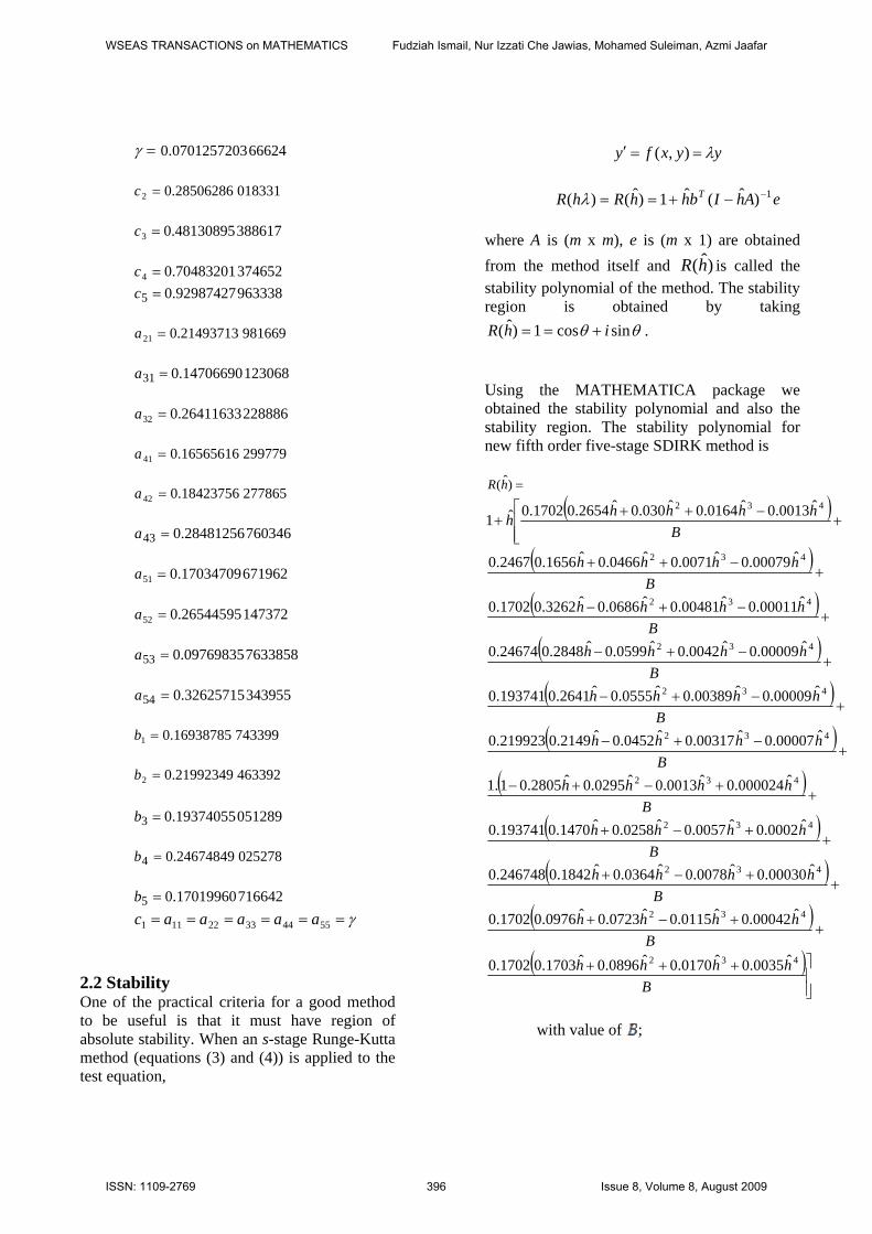
s the imaginary part and the horizontal axis is the real part.

Mathematica package (see Torrence [11]). The stability region is obtained by tracing the values of h and is shown in Figure 1. Where the vertical axis i

- 10 - 5 0 5 10

- 7.5

- 5

- 2.5

0

2.5

5

7.5

Real Part

ImaginaryPart StabilityRegion

Figu

order 5-stage SDIRK method

Zingg and Chisholm [13] is discussed below;

the SDIRK method and the stability polynomial

for the explicit method is denoted by

here

Equating

re 1: The stability region for the 5th

The stability analysis for fifth order five-stage explicit Runge-Kutta (ERK5) method which has been derived by

Where the stability polynomial is obtained as in

hR1 ,

w

)ˆ(1 hR

022377.0

372401.0

372401.0

02505.0(

040921.0

09957.0

.1(ˆ1 h

))ˆ

ˆ01157.0ˆ0407.0ˆ08886.0(

)ˆ1065.0ˆ10238.0ˆ2630.0(

)ˆ05682.0ˆ003002.0ˆ04092.0)ˆ2706.0ˆ13437.0(

)ˆ2247.0ˆ1043.0(3724.0)ˆ

ˆ04418.0(41041.0ˆ3527.0

4

32

32

32

2

22

h

hhh

hhh

hhh

hh

hhh

hh

)ˆ(hR1 sincos1 i

and solving for h we h

ave the stabilty the method.

regoin of

- 4 - 3 - 2 - 1 0 1- 4

- 2

0

2

4

Real Part

ImaginaryPart StabilityRegion

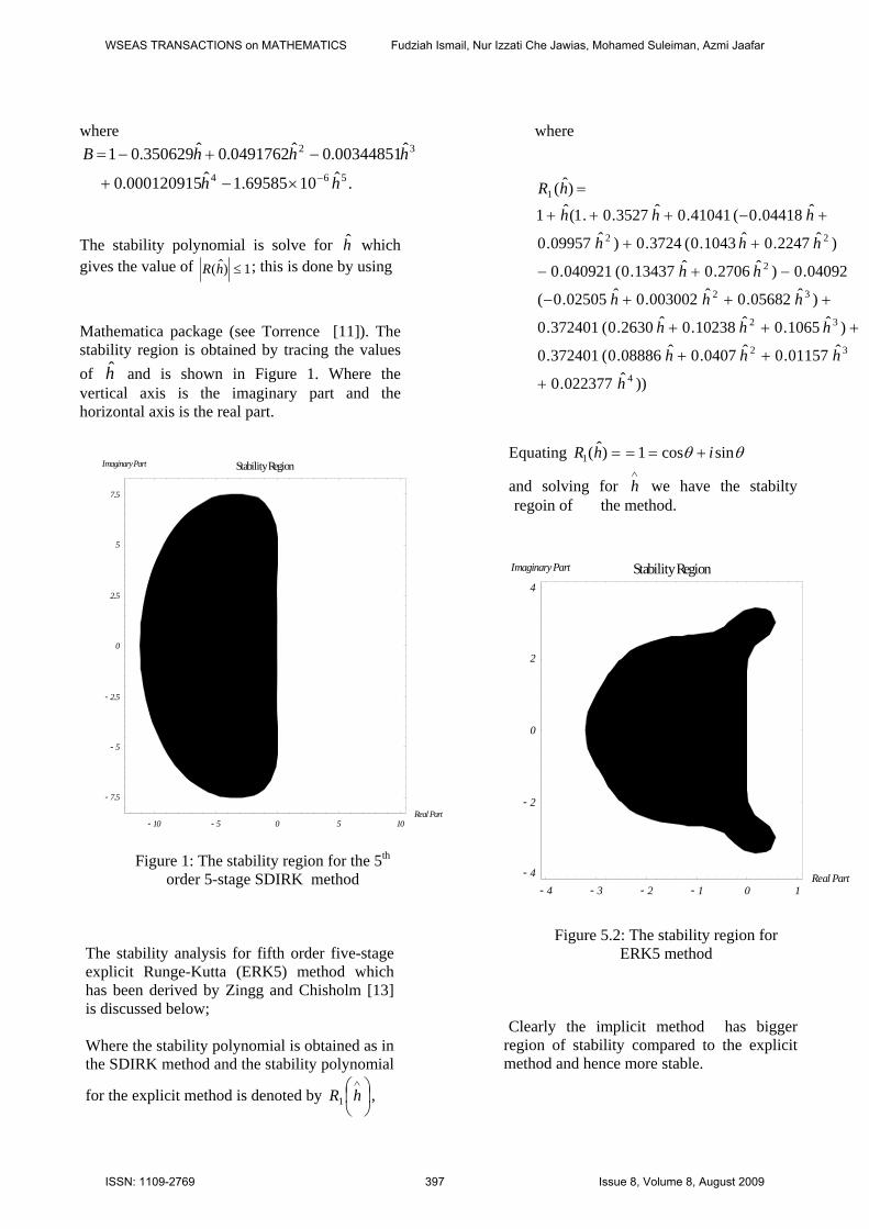
Figure 5.2 egion for ERK5 method

the explicit method and hence more stable.

: The stability r

Clearly the implicit method has bigger region of stability compared to



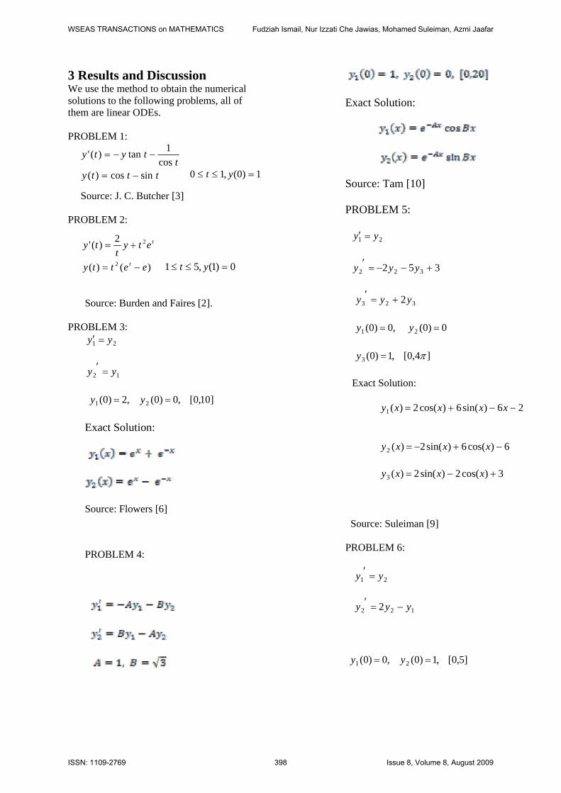
3 Results and Discussion We use the method to obtain the numericalsolutions to the followin

g problems, all of

3]

R

rden and Faires [2].

PROBLEM 3:

them are linear ODEs.

PROBLEM 1:

Source: J. C. Butcher [

P OBLEM 2:

Source: Bu

21 yy

12 yy

,2)0( ]10,0[,0)0(21 y y

Exact Solution:

Source: Flowers [6]

PROBLEM 4:

Exact Solution:

Source: Tam [10]

OBL : PR EM 5

21 yy

33 52 22 yy y

323 2yyy

0)0(,0)0( 21 yy

4,0[,1)0(3 ]y

Exact Solution:

26)sin(6)cos(2)(1 xxxx

6)cos(6)sin(2)(2

y

xxxy

3)s()(3 co2)sin(2 x xxy

an [9]

OBLEM :

Source: Suleim

PR 6

21 yy

22 2yy 1y

]5,0[,1)0(,0)0( 21 yy

ttty sincos)( t

tytycos

1tan)( '

1)0(,10 yt

)()( 2 eett

etyt

ty

t

t

2)(' 2

y 0)1(,51 yt



Exa nct Solutio :

y xxex )(1

xexxy )1()(2

Source: Bronson [1]

abulated and compared with the existing method and

w are the notations used:

ed

computed solution

The numerical results are t

belo

H ~ Step size used

MTHD ~ Method employ

MAXE ~Maximum error The true solution minus the : ii yxy )(

SDIRK5L ~ New fifth order five- d

with minimized error norm for LODEs.

od for LODEs (Zingg and Chisholm, [13])

SD

five-stage SDIRK (Ferracina and Spijker, [5])

able rical r lts for p 1

MT D MAXE

stage SDIRK metho ERK5 ~ Fifth order five-stage explicit RK meth

IRK4(II)~ Optimal fourth order

T 3: Nume esu roblem

H

H

SDIRK5L

0. 1 6.12153e-009

1. ER 5 4.73152e-007 K SDIR 4 (II) 4.90905e-008 K

SDIRK5L 0. 05 9.68726e-011 2. ER 5 6.28651e-008 K SDIR 4 (II) 2.04009e-009 K

SDIRK5L 0.025 5.51288e-012 3. ER 5 8.05691e-009 K SDIR 4 (II) 1.24309e-010 K

SDIRK5L 0. 01 1.32783e-013 4. ER 5 5.22694e-010 K SDIR 4 (II) 3.97293e-012 K

SDIRK5L 0.005 7.76462e-015 5. ER 5 6.56258e-011 K SDIR 4 (II) 1.06698e-012 K

SDIRK5L 0.0 5 02 1.14908e-014 6. ER 5 8.21701e-012 K SDIR 4 (II) 8.74190e-013 K

SDIRK5L 0.001 4.44089e-016 7. ERK5 5.27051e-013 SDIRK4 (II) 8.74356e-013



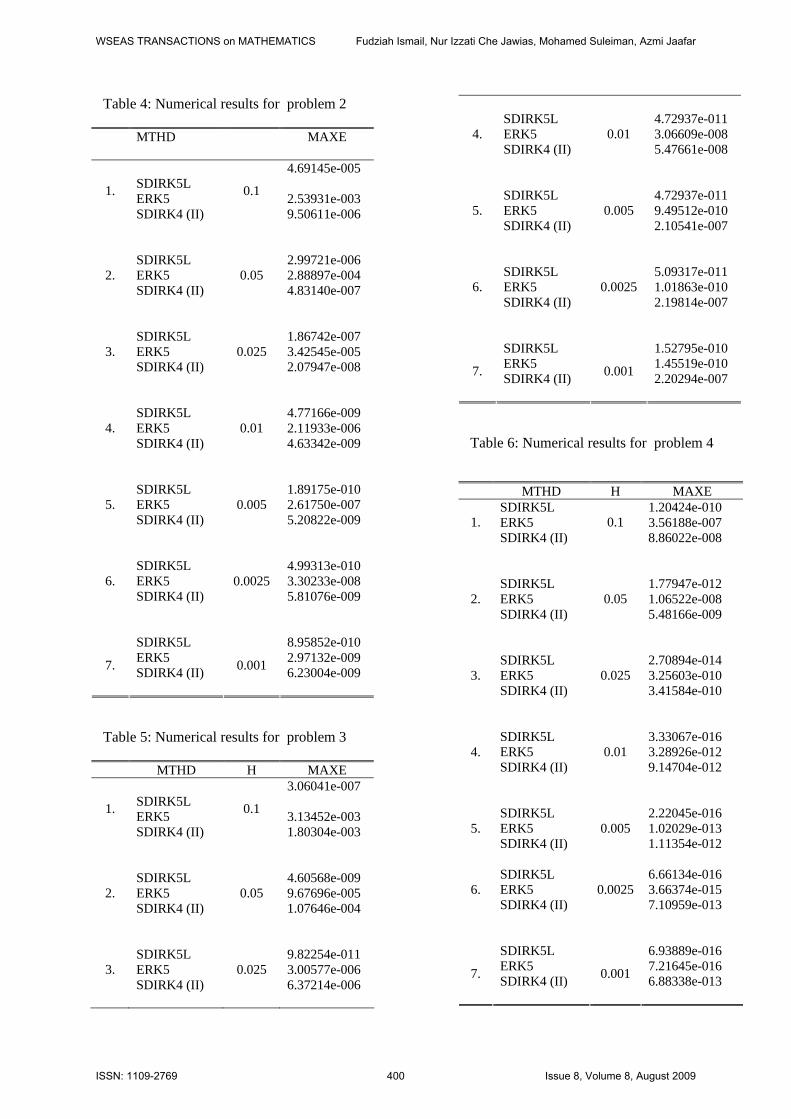
T ble erical results for pro

MTHD

a 4: Num blem 2

MAXE

SDIRK5L

4.69145e-005

ERK5 2.53931e-003 1.

DIRK4 (II)

0.1

9.50611e-006

RK5 2.88897e-004 DIRK4 (II)

0. 4.83140e-007

RK5 3.42545e-005 DIRK4 (II)

0.025 2.07947e-008

RK5 2.11933e-006 DIRK4 (II)

0. 4.63342e-009

RK5 2.61750e-007 DIRK4 (II)

0.005 5.20822e-009

RK5 3.30233e-008 DIRK4 (II)

0.0 5 5.81076e-009

RK5 2.97132e-009 7. SDIRK4 (II)

0.001 6.23004e-009

S

SDIRK5L 2.99721e-006 E2. S

05

SDIRK5L 1.86742e-007 E3. S

SDIRK5L 4.77166e-009 E4. S

01

SDIRK5L 1.89175e-010 E5. S

SDIRK5L 4.99313e-010 E6. S

02

SDIRK5L 8.95852e-010 E

T ble 5: al resu for pro

MAXE

a Numeric lts blem 3

MTHD H SDIRK5L

3.06041e-007

ERK5 3.13452e-003 1.

DIRK4 (II)

0.1

1.80304e-003

RK5 9.67696e-005 DIRK4 (II)

0. 1.07646e-004

RK5 3.00577e-006 DIRK4 (II)

0.025 6.37214e-006

S

SDIRK5L 4.60568e-009 E2. S

05

SDIRK5L 9.82254e-011 E3. S

SDIRK5L .72937e-011

RK5 3.06609e-008 )

0. 1

DIRK5L .72937e-011 RK5 9.49512e-010

) 0.005

DIRK5L .09317e-011 RK5 1.01863e-010

) 0.0 25

SDIRK5L .52795e-010 ERK5 1.45519e-010 SDIRK4 (II) 0.001 2.20294e-007

4E4. SDIRK4 (II

05.47661e-008

S 4E5. SDIRK4 (II 2.10541e-007

S 5E6. SDIRK4 (II

02.19814e-007

1

7.

T ble 6: cal resu for pro

H

a Numeri lts blem 4

MTHD MAXE SDIRK5L .20424e-010 1ERK5 3.56188e-007 1.

0

DIRK5L .77947e-012 RK5 1.06522e-008 2.

0.

DIRK5L .70894e-014 ERK5 3.25603e-010 3.

0.025

DIRK5L .33067e-016 RK5 3.28926e-012 4.

0.

DIRK5L .22045e-016 5.

4 (II) 0.005

DIRK5L .66134e-016 RK5 3.66374e-015 6.

0.0 5

SDIRK5L .93889e-016 ERK5 7.21645e-016

SDIRK4 (II).1

8.86022e-008

S 1ESDIRK4 (II)

055.48166e-009

S 2

SDIRK4 (II) 3.41584e-010

S 3ESDIRK4 (II)

019.14704e-012

S 2ERK5 1.02029e-013 SDIRK 1.11354e-012 S 6ESDIRK4 (II)

027.10959e-013

6

7. SDIRK4 (II) 0.001 6.88338e-013



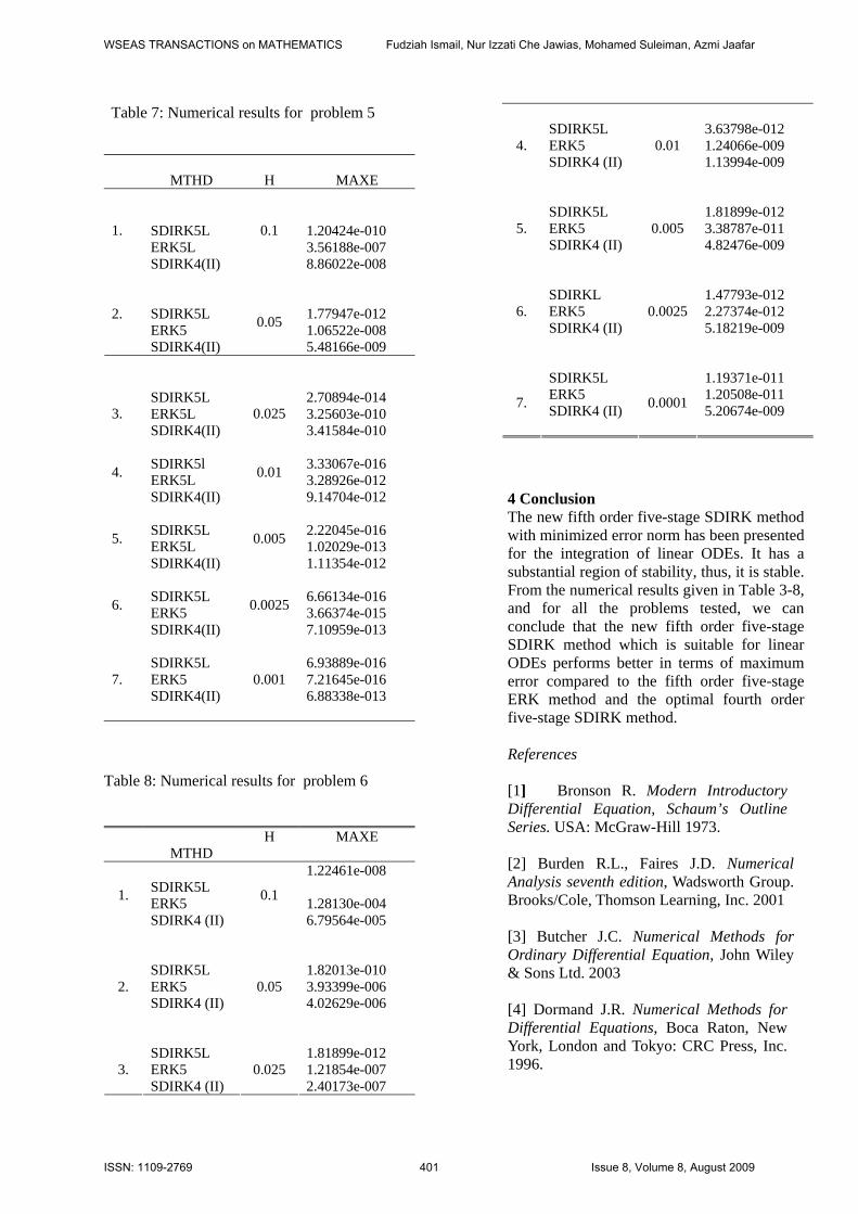
Table 7: Nu m

merical results for proble 5

MTHD H MAXE SDIRK5L .20424e-010

1

ERK5L 3.56188e-007 1.

0.1

DIRK5L .77947e-012 RK5 1.06522e-008

2.

0.

DIRK5L .70894e-014

SDIRK4(II) 8.86022e-008 S

1

ESDIRK4(II)

05

5.48166e-009 S

2

ERK5L 3.25603e-010

I)

DIRK5l .33067e-016 4.

I)

0.01

DIRK5L .22045e-016 5.

4(II)

0.005

DIRK5L .66134e-016 6.

4(II)

0.0025

SDIRK5L .93889e-016 RK5 7.21645e-016 .

SDIRK4(II) 0.001

6.88338e-013

3. SDIRK4(I

0.025 3.41584e-010

S

3

ERK5L 3.28926e-012 SDIRK4(I 9.14704e-012 S

2

ERK5L 1.02029e-013 SDIRK 1.11354e-012 S

6

ERK5 3.66374e-015 SDIRK 7.10959e-013

6E7

Ta e 8: Num rical resul or prob

MAXE

bl e ts f lem 6

MTHD

H

SDIRK5L

1.22461e-008

ERK5 1.28130e-004 1.

0

DIRK5L 1.82013e-010 RK5 3.93399e-006 2.

0.

DIRK5L 1.81899e-012 3.

4 (II) 0.025

SDIRK4 (II)

.1

6.79564e-005

SESDIRK4 (II)

05 4.02629e-006

SERK5 1.21854e-007 SDIRK 2.40173e-007

SDIRK5L 3.63798e-012

4. 4 (II)

0.01

DIRK5L 1.81899e-012 5.

4 (II) 0.005

DIRKL 1.47793e-012 6.

4 (II) 0.0025

SDIRK5L 1.19371e-011 ERK5 1.20508e-011 7. SDIRK4 (II) 0.0001 5.20674e-009

ERK5 1.24066e-009 SDIRK 1.13994e-009

SERK5 3.38787e-011 SDIRK 4.82476e-009

SERK5 2.27374e-012 SDIRK 5.18219e-009

4 Conclusion The new fifth order five-stage SDIRK method with minimized error norm has been presented for the integration of linear ODEs. It has a substantial region of stability, thus, it is stable. From the numerical results given in Table 3-8, and for all the problems tested, we can conclude that the new fifth order five-stage SDIRK method which is suitable for linear ODEs performs better in terms of maximum

ed to the fifth order five-stage d and the optimal fourth order

rmand J.R. Numerical Methods for Dif ential Equations, Boca Raton, New

error comparRK methoE

five-stage SDIRK method.

References [1] Bronson R. Modern Introductory Differential Equation, Schaum’s Outline Series. USA: McGraw-Hill 1973. [2] Burden R.L., Faires J.D. Numerical Analysis seventh edition, Wadsworth Group. Brooks/Cole, Thomson Learning, Inc. 2001

[3] Butcher J.C. Numerical Methods for Ordinary Differential Equation, John Wiley & Sons Ltd. 2003

[4] Do

ferYork, London and Tokyo: CRC Press, Inc. 1996.



f Singly-Diagonally-Implicit unge-Kutta methods. Report no MI 2007-

] Flowers, B. H An Introduction to

Twice Nonlinearity in class of Discontinuous Functions, WSEAS

Traffic Flow in a class f Discontinuous Functions, WSEAS

lving Higher Order DEs Directly by Direct Integration

l Methods for the Numerical Solution of

nce B.F., Torrence E.A.: How to nd the stability regions, The Student’s

ree Boundary Convective Mass Transfer

unge-Kutta methods for linear ordinary differential equations, Applied Numerical Mathematics. 31, 1999, pp. 227-238.

[5] Ferracina L., Spijker M.N. Strong stability oR11, 2007, Mathematical Institute, Leiden University. [6Numerical Methods in C+ +, New York: University Oxford Press 2000. [7] Rasulov, R and Kul, R. H. Numerical Solution of One Dimensional Nonlinear Wave Equation withaTransactions on Mathematics, vol 5, no 12, 2006, : 1336-1338. [8] Rasulov, M, Sinsoyal, B. and Hayta, S. Numerical Simulation and Initial-Boundary Value Problems for oTransactions on Mathematics, vol 5, no 12, 2006, : 1339-1342. [9] Suleiman M. B. SoOMethod, Applied Math. And Computation. 33(3), 1989: 197-219. [10] Tam, H. W. Two-stage Paralle

Ordinary Differential Equations, Siam J. Sci. Stat. Comput. 13(5, 1992: 1062-1084

[11] TorrefiIntroduction to Mathematica, 1999, pp. 232-264. [12] Zabala, D. and Ramos, A. L. Effect of the Finite Difference Solution Scheme in aFModel, WSEAS Transactions on Mathematics, vol 6, no 6, 2007, : 693-700. [13] Zingg D.W., Chisholm T.T. R



Solving Linear Ordinary Differential Equations using Singly Diagonally Implicit Runge-Kutta fifth...

Documents

Transcript of Solving Linear Ordinary Differential Equations using Singly Diagonally Implicit Runge-Kutta fifth...