Ann. Inst. Statist. Math. Vol. 46, No. 1, 5~66 (1994)

THE SINGLY TRUNCATED NORMAL DISTRIBUTION: A NON-STEEP EXPONENTIAL FAMILY

JOAN DEL CASTILLO

Department of Mathematics, Universitat Aut6noma de Barcelona, 08192 BeIlaterra, Barcelona, Spain

(Received September 17, 1992; revised January 21, 1993)

Abst rac t . This paper is concerned with the maximum likelihood estimation problem for the singly truncated normal family of distributions. Necessary and suficient conditions, in terms of the coefficient of variation, are provided in order to obtain a solution to the likelihood equations. Furthermore, the maximum likelihood estimator is obtained as a limit case when the likelihood equation has no solution.

Key words and phrases: Truncated normal distribution, likelihood equation, exponential families.

1. Introduction

Truncated samples of normal distribution arise, in practice, with various types of experimental data in which recorded measurements are available over only a partial range of the variable. The maximum likelihood estimation for singly trun- cated and doubly truncated normal distribution was considered by Cohen (1950, 1991). Numerical solutions to the estimators of the mean and variance for singly truncated samples were computed with an auxiliar function which is tabulated in Cohen (1961). However, the condition in which there is a solution have not been determined analytically.

Barndorff-Nielsen (1978) considered the description of the maximum likeli- hood estimator for the doubly truncated normal family of distributions, from the point of view of exponential families. The doubly truncated normal family is an example of a regular exponential family. In this paper we use the theory of convex duality applied to exponential families by Barndorff-Nielsen as a way to clarify the estimation problems related to the maximum likelihood estimation for the singly truncated normal family, see also Rockafellar (1970).

The singly truncated normal family of distributions is a natural and practical example of a non-regular and non-steep exponential family; for more information see Efron (1978) and Letac and Mora (1990). The complete description of the mean domain of this family is given in Theorem 4.2, that shows likelihood equation,

57

58 JOAN DEL CASTILLO

solved numerically by Cohen, has only one solution if and only if the sample coefficient of variat ion is less than 1. If the sample coefficient of variat ion is greater than 1, which happens with positive probability, then the max imum likelihood est imator yields a distr ibution of the usual one-parameter exponential family. In the paper we also give numerical functions defined in M A T H E M A T I C A which provided the solutions to the likelihood equations, and a short table, computed with these functions, which can be used to obtain a first approximat ion to the solutions. Wi thou t loss of generality, only distr ibutions left t runca ted by zero are considered. The usual changes a - z z for a random variate z, left t runca ted by zz, or z~ - z for a r andom variate z, right t runca ted by z~, can be used to reduce the problem to the previous situation.

2. Exponential families

Let # be a ~-finite positive measure on a ~-algebra of subsets of a measurable space X and let T be a statistic on 32 over Nk. Let #T be the marginal dis tr ibut ion of T and let us consider its Laplace transform

LT(O)= /~ve°tT d#= £ke°hd#T , 0 ~ ~ ~.

We denote the existence domain of LT by D = {0 : LT(O) < oc} (which is convex, by H/51der's inequality) and the interior of D by (9 = int(D), which we will assume is not empty.

Let us consider the family of distributions

79D = {p(z; O)d# = eo*r(z)-~:T(O)d# : 0 C D}

where KT(O) = in Lr(O) is a str ict ly convex function on 0 , from H/51der's inequal- ity, and real analyt ic on 0 . The family PD is called a full ezponential family and D is called its natural parameter space. 79D is said to be regular if D = @; if not then we will also consider 79e = {p(z; O)d# : 0 E 0} . Let S be the suppor t of the measure #T and let C be the closed convex hull of S. Let us assume tha t S is not included in an affine submanifold of R k. Then T is a minimal sufficient statist ic for family 799 .

For 0 E 6), the mean value and the covariance mat r ix of T can be obta ined by differentiation

(2.1) CgKT EoT - -

O 0 '

VoT = 02KT 0000'"

Since KT is str ict ly convex on (9, the map r(0) = EoT is one-to-one. Denote by Mr the image of 0 by T; MT is refered to as the domain of means of P c . Clearly, Mr is included in the interior Of C. If MT = int(C) then family 79D is said to be steep. In most of the cases the full exponential families are regular or

THE SINGLY TRUNCATED NORMAL DISTRIBUTION 59

steep, but not always, as we shall see in Section 4 (see also Efron (1978) and Letac and Mora (1990)).

Let x = (xl, x2 , . . . , x~)t be a random sample of a distr ibution p(x; O)d# • Pp. The log-likelihood function for the family 7)D is

(2.2) l(0; ~) : ~ ( 0 * t - K~(0)) , 0 • D

7% where t = }-~4=~ T(x{)/n. Then, the likelihood equations for a full exponential family are

(2.3) ~-(0) = EoT = t, 0 • O.

Note tha t the likelihood est imation method for 0 • O corresponds to the method of moments for the statistic T. The function Ott - KT(O ) is the Legendre t ransform of KT(O) and the conjugate of the convex function KT(O)

(2.4) [(t) = sup{0t t - K(0)} OED

is called the sup-log-likelihood function (see Barndorff-Nielsen (1978)).

The effective domain, of [(t) is the set dom(/) = {t : [(t) < +oc} which corresponds to the set of points for which maximum likelihood est imate exist. The following result gives us a good approximation of dom(/); its proof can be found in Barndorff-Nielsen ((1978), p. 140).

THEOREM 2.1. With the notations given above, we have

int(C) c dora(l) c c,

in particular, for a random sample x = (xl, x2 , . . . , x~) t, if t = ~ T (x i ) / n is in int(C) then there is a maximum of the likelihood function l(O, x) on D.

3. The truncated normal distribution

Let us consider the full exponential family ~)D given by X = ~+, dp(x) = dx the Lebesgue measure on ~+ and T(x) = (x , - x2) . The Laplace t ransform of PT is

f0 ° (3.1) LT(01,02) = eOlx-02X~dz ' (01,02) • ~2

straighforward integration shows tha t LT(01,02) is finite on D = O U 00, where (9 = int(D) = N x N+ and Oo = {(0,0) : 0 < 0}, and we have

(3.2) L~(O~, o2) : ~¢(Ol/ vff~)e °~ /4°2,

1 LT(O,O) : - g , (0,0) e eo

(01,02) 6 0 ,

60 JOAN DEL CASTILLO

where 0(a) is the distr ibution function of the s tandard normal. Let us consider for (01,02) E O, the parametr izat ion 01 = #/(72 and 02 =

1/2(72, then the probabil i ty density functions of distributions of 7)0 are

(3.3) p(x; 01, 02) = ( , / ~ 0 ( ~ / ~ ) ) - 1 e x p ( - ( x - ~ ) 2 / 2 £ ) , 0 < x < ~ ,

which shows that 7)e is the family of singly truncated normal distributions (see Cohen (1991)). On the other hand, we can consider the family 7)0o of the distri- butions of PD with parameters (0, 0) E 0o. Clearly 7)Oo is the usual one-parameter exponential family of distributions.

(3.4) p(x;O,O) = -Oe °x, 0 < 0 , O < x < oe.

Now, we shall s tudy the regularity of KT(01, Oz) = tnLT(O1,02) on D. To this end we introduce some notation. Let

/7 K(x) = in ext=t2/4dt, x E R

then K(x) is a convex function, since it is the logarithm of a Laplace transform, and KT(01,02) = -- ln(2v/-~2) + K(O1/2x/-O~2). Let k(x) be the derivative of K(x). The following expressions are available for k(x).

k(~) = 2~ + e - ~ / z ( ~ ) : 2~ + e - ~ ( ~ / ~ , ( ~ x ) ) -~ : 2~ + vS/R(-~)

where E(x) = v ~ ( g ~ x ) is the error function and R(x) : ~ 0 ( - x ) e x2/2 is the Mills' ratio.

Note that for (01,02) E O the m a p T(Oi ,02) ~- E(ol,o~)(T); 7 = (T1, T2) t, may be expressed as

OKT _ _ o~_ lxk (x ) ' T1(01'02) -- 001

(3.5) ~-2(ol e2) - OKT _ _20~2(x2 + x3k(x))

' 002

where x = 01/2x/022.

PROPOSITION 3.1. (a) The functions LT(O1,02) and KT(01,02) are C 1 func- tions on D = (9 U (9o, with

OKT OKT (0, O) = O -1, (0, O) = - 2 0 -2. OO1 002

(b) The probability density function p(X;Ol,02), (01,02) E (9, converges to p(x;O,O), (0,0) E (90, in Ll(~+dx) as (01,02) tends to (0,0).

PROOF. LT(01, 02) and KT(01,02) be real analytic on (9, then let us assume (0~,02) is in a neighborhood of (0,0), 0 < 0. If (01,02) tends to (0,0), then e x p ( 0 1 x - 0 2 x 2) converges to exp(0x) for all x in [9+ and for some e > 0, 0 + e < 0,

(3.6) I exp(01x - 02x2)1 <_ exp((0 + e)x).

THE SINGLY TRUNCATED NORMAL DISTRIBUTION 61

Prom the Lebesgue bounded convergence theorem it follows that LT(01,02) and KT(01 ,02) are continuous in D. The continuity of LT(O1,02) and the inequality (3.6) also prove (b), by Lebesgue bounded convergence theorem.

When x tends to - o c we can show the following limits hold

(3.7) lira x k ( x ) = - 1 , lim ( x3k (x ) + x2) = 1. 3 ? - - > - - 0 0 37---~ - - O ~

If (01,02) tends to (0, 0) then x = 01/2N~2 tends to - o o and, from (3.5), we deduce that (?-1,72) tends to (0 -1, - 2 0 - 2 ) . This show that mapping (?-1,72), defined on 0 , can be extended continuously to O0 and LT(O1,02) and KT(01 ,0~) are in CI(D).

prom this proposit ion it now follows that family 79D is not a steep family, tha t is, the maximum likelihood est imate is not always a solution to likelihood equations (see Barndorff-Nielsen (1978)), but we shall show this directly in the next section.

4. Maximum likelihood estimates

Let x = ( X l , X 2 , . . . , xn ) , be a random sample of a distr ibution of 79D. Let n

t l = ~J-~i=l x i / n , tz = - 2 x~ /n . Then (ta, t2) E C where

(4.1) C = {(x,y) ~ N 2 : x > 0, y _< -x2} ,

because C is convex, and ( t l , t2) E int(C) with probabil i ty one, because n > 1. If ( t l , t2) E int(C) we know, from Theorem 2.1, tha t there is a maximum likelihood est imate (01,02) in D. We note tha t if (01,02) is a solution of the likelihood equations (2.3), where ?- = (?-1, ~-2)t is given in (3.5), then (01,02) E (9 and the maximum likelihood est imate is a distr ibution of the singly t runcated normal family, 7)0. In this case, we can express the likelihood equations in terms of parameters # = 0 1 / 2 0 2 , o -2 = 1/202 by

E ( t l ) = = t l ,

(4.2) V ~

E ( t 2 ) = _ o - 2 _ = t 2 .

In part icular we see that likelihood equations correspond to est imations by the method of moments.

If (tl, t2) is not included in the domain of means of 79e, ?-(O), then (01,02) E 00 and the maximum likelihood est imate is a distr ibution of the usual one-parameter exponential family.

PROPOSITION 4.1. Let s 2 = - ( t 2 + t~), the s tandard deviation, and c = s / t l , the sample coefficient of variation. The likelihood equations (4.2) are equivalent to the equation

(4.3) (1 + c2)k(x) 2 - 2 x k ( x ) - 2z = O, z E [R

62 JOAN DEL CASTILLO

~ i t h C, = , / f f t l / k ( ~ ) and ~ = 2 t l~ /k (~ ) .

PROOF. If x = #/X/-2cr then, from (4.2), we have

t ~ k ( ~ ) _ 2 (1 + e~)k(~) = - ~ - k(x--U + 2~

and this equat ion is equivalent to (4.3). Also from (4.2), we have cr = ~ t l / k ( x ) and then # = x/2crx = 2tex/k(x). []

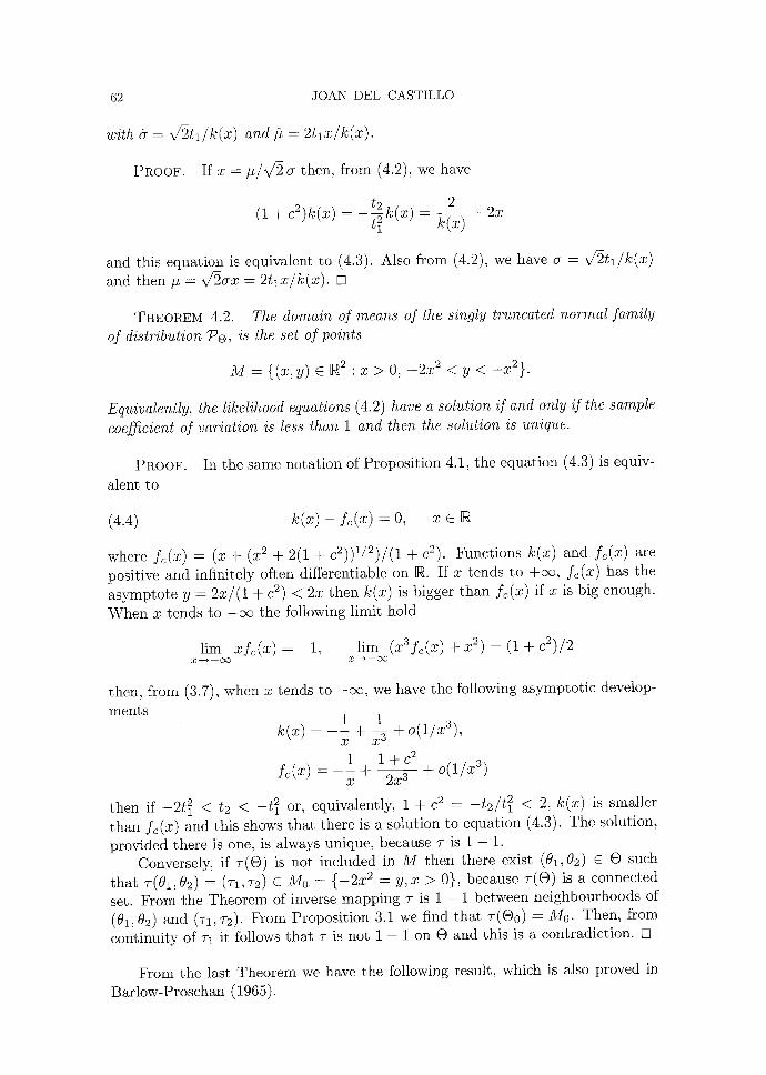
THEOREM 4.2. The domain of means of the singly truncated normal family of distribution 7)e, is the set of points

M = { (x ,y ) • a ~ : x > 0, - 2 ~ 2 < y < - ~ 2 } .

Equivalently, the likelihood equations (4.2) have a solution if and only if the sample coefficient of variation is less than 1 and then the solution is unique.

PROOF. In the same nota t ion of Proposi t ion 4.1, the equat ion (4.3) is equiv-

alent to

(4.4) k(~) - L ( ~ ) = O, • e

where fc(x) = (x + (x 2 + 2(1 + c2))U2)/(1 + c2). Functions k(x) and fc(x) are positive and infinitely often differentiable on R. If x tends to +oo, fc(x) has the asympto te y = 2x/(1 + c 2) < 2x then k(x) is bigger than fc(x) if x is big enough.

When x tends to - o c the following limit hold

lim x f c ( x ) = - 1 , X----~ -- OO

lim (x3f~(x) + x 2) = (1 + e2)/2 X--->-- O0

then, from (3.7), when x tends to - o c , we have the following asymptot ic develop-

ments 1 1 k ( ~ ) = - - + + o ( 1 / x a ) ,

x J i i +c 2

_ _ + - - + o ( 1 / x ~) f~(x) ---- x 2x 3

then if - 2 t l 2 < t2 < - t~ or, equivalently, 1 + c 2 = -t2/t~ < 2, k(x) is smaller than fc(x) and this shows tha t there is a solution to equation (4.3). The solution, provided there is one, is always unique, because ~- is 1 - 1.

Conversely, if 7-(@) is not included in M then there exist (01,02) E O such tha t 7 - ( 0 1 , 0 2 ) = (T1, 7-2) E M 0 = { - 2 x 2 = y , x ) 0 } , because 7-(0) is a connected set. From the Theorem of inverse mapping 7- is 1 - 1 between neighbourhoods of (01,02) and (7-1,7-2). From Proposi t ion 3.1 we find tha t 7-(0o) = M0. Then, from continuity of 7-1 it follows tha t 7- is not 1 - 1 on • and this is a contradict ion. []

From the last Theorem we have the following result, which is also proved in

Barlow-Proschan (1965).

THE SINGLY TRUNCATED NORMAL DISTRIBUTION 63

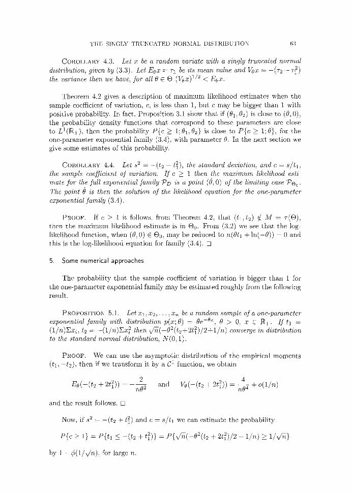
COROLLARY 4.3. Let x be a random variate with a singly truncated normal distribution, given by (3.3). Let Eox = 71 be its mean value and Voz = -@2 + T~) the variance then we have, for all 0 E (9 (Voz) 1/2 < Eox.

Theorem 4.2 gives a description of maximum likelihood estimates when the sample coefficient of variation, c, is less than 1, but c may be bigger than 1 with positive probability. In fact, Proposition 3.1 show that if (01,02) is close to (0, 0), the probability density functions that correspond to these parameters are close to LI(•+), then the probability P{c >_ 1;02,02} is close to P{c >_ 1;0}, for the one-parameter exponential family (3.4), with parameter 0. In the next section we give some estimates of this probability.

COROLLARY 4.4. Let s 2 = - ( t z + t~), the standard deviation, and c = s / t l , the sample coefficient of variation. I f c >_ 1 then the mazimum likelihood esti- mate for the full ezponential family PD is a point (0, O) of the limiting case Peo. The point 0 is then the solution of the likelihood equation for the one-parameter ezponentiaI family (3.4).

PROOF. If c _> 1 it follows, from Theorem 4.2, that (tl, t2) ~ M = v-((~), then the maximum likelihood estimate is in O0. From (3.2) we see that the log- likelihood function, when (0, 0) E O0, may be reduced to n(Oh + ln(-0)) = 0 and this is the log-likelihood equation for family (3.4). []

5. Some numerical approaches

The probability that the sample coefficient of variation is bigger than 1 for the one-parameter exponential family may be estimated roughly from the following result.

PROPOSITION 5.1. Let z l , z2, . . . , zn be a random sample of a one-parameter ezponential family with distribution p(z; O) = Oe -°z , 0 > O, x c R+. I f t~ = (1 /n)Ezi , t2 = - ( 1 / n ) E z 2 then , fn( -O2( t2+2t~) /2+ l / n ) converge in distribution to the standard normal distribution, N(O, 1).

PROOF. We can use the asymptotic distribution of the empirical moments @1, - t2) , then if we transform it by a C 1 function, we obtain

Eo(- ( t~ + 2t12)) _ nO 22 and Vo(-(t2 + 2t~)) = ~ 4 + o(1/n)

and the result follows. []

Now, if s 2 = - ( t2 + t~) and c = s/t1 we can estimate the probability

P{c >_ 1} = P{t l <_ - ( t2 + t~)} : P{x/~(-02(t2 + 2t~)/2 + i /n ) > 1/~ff~}

by 1 - ¢(i/x/~), for large n.

64 JOAN DEL CASTILLO

For small samples we have est imated the probability P { c >_ 1}, for the one- parameter exponential family by simulation. We used 5,000 random samples of size n, for n = 10, 20, 30, 50 from a generator of MATHEMATICA and we obtained the following table.

Table 1. Approximate values for P{c >_ 1}.

r~ 10 20 30 40 50 P{c > 1} ~ 0.254 0.319 0.347 0.352 0.364 1-~(1/x/~) 0.376 0.412 0.478 0.437 0.444

When the sample coefficient of variation, c, is less than 1, the solution to the likelihood equation (4.2) can be obtained, of course, using the auxiliary function 0(7), where 7 = c2, which is tabulated by Cohen (1961). Then, the solution is

12 = 2(1 - 0(c2)), ~ = s 2 + 0(c2)~ 2

where 2 and s are the sample mean and the s tandard deviation. The relationship between O(c 2) and the solution x(c) to the equation (4.3), or equivalently (4.4), is given by

c 2 + O(c 2) 2 z ( c ) 2 -

(1 - 0(c2)) 2

The solution to (4.2) can also be obtained from the equation (4.4) and the functions mu[m, s] and sigma[m, s] defined in MATHEMATICA by

k[x_] := 2z + (2/Sqrt[Pi])E(-zA2)/Erf[-infinity, z];

f[x_, c_] := (z + Sqrt[xA2 + 2(1 + cA2)1/(1 + cA2);

z[c_] := x/.FindRoor[k[z] - f[z, c], {x, { - 1 0 , 10}}, AccuracyGoal --* 10];

sigma[m_, s_] := Sqrt[2]m/k[z[s/m]]//N, mu[m_, s_] := 2 m x [ s / m ] / k [ x [ s / m ] ] / / N ,

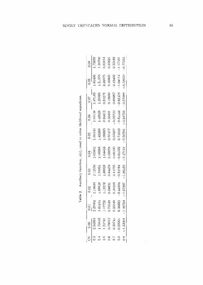
where m = 2 = t l and s = - ( t2 + t~) 1/2. In order to facilitate a first est imation of t runcated normal distr ibution we

give Table 2, which expresses the solution z(c), to the equation (4.4) when the coefficient of variation c ranges between 0.30 and 0.99. Table 2 has been computed using the last function x[c]. From Table 2 we can find the maximum likelihood est imation for parameters #, cr of the t runcated normal family by

= ~ / f c ( x ( c ) ) , /2 = ~ ( ~ )

where fc(x) = (z + (z 2 + 2(1 + C2))1/2)/(1 -~- C2), because z(c) is a solution of equation (4.4).

SINGLY T R U N C A T E D NORMAL DISTRIBUTION 65

© ©

.o.

;~ .~

:.~ .~

<

N

,.~

¢

~ ~ ~ ~ ~

~ ~ ~ ~ L© ~ ~ ~ ~ ~ ~ ~ ~ ~

~ d ~ ~

~ ~ ~ ~ ~ ~

~ ~ ~ ~ ~

• ~ ~

e ~ d d d ~ I

~ ~ ~ ~ ~ ~

~ 2 N ~ N ~ N ~ . ~ ~ ~

~ . . . . . . . ~ ~ ~

~ ~ ~ ~ ~ ~

~ N ~ ~ . ~ ~ ~

~ . . . . . . . ~ ~ ~

I

~ ~ ~ ~ ~ ~

~ ~ g ~ . ~ ~ ~

~ . . . . . . . ~ ~ ~

~ ~ ~ ~ ~ ~

" ~ N ~ ; ~ ~ ~ ~ N ~ d d d N

~ ~ ~ ~ ~ ~

~ ~ g ~ . ~ ~ ~

~ . . . . . . . ~ ~ ~

~ ~ ~ ~ ~ ~

~ ~ ~ . ~ ~ ~

~ N ~ d d d ~ l

~ ~ ~ ~ ~ ~

~ ~ ~ . ~ ~ ~

~ . . . . . . . ~ ~ ~

I

~ ~ ~ ~ ~ ~

~ ~ ~ ~ ~

~ ~ ~ ~ . . . . . . .

~ ~ ~ I

~ ~ ~ ~ d d d d d d d

66 JOAN DEL CASTILLO

REFERENCES

Barlow, R. and Proschan, F. (1975). Statistical Theory of Reliability and Life Testing, Holt Rinehart and Winston, New York.

Barndorff-Nielsen, O. (1978). Information and Exponential Families, Wiley, Norwich. Cohen, A. C. (1950). Estimating the mean and variance of normal populations from singly

truncated and doubly truncated samples, Ann. Math. Statist., 21, 557-569. Cohen, A. C. (1961). Tables for maximum likelihood estimates: singly truncated and singly

censored samples, Technometrics, 3, 535-541. Cohen, A. C. (1991). T~ncated and Censored Samples, Marcel Dekker, New York. Efron, B. (1978). The geometry of exponential families, Ann. Statist., 6, 362 376. Letac, G. and Mora, M. (1990). Natural real exponential families with cubic variance functions,

Ann. Statist., 18, 1-37. Rockafellar, R. (1970). Convex Analysis, Princeton University Press, New Jersey.