Fire and plant interactions in forested ecosystems of south-west Western Australia

DAYTIME TURBULENCE STATISTICS ABOVE A STEEP FORESTEDSLOPE
E. VAN GORSEL, A. CHRISTEN, C. FEIGENWINTER, E. PARLOW and R. VOGTInstitute of Meteorology, Climatology and Remote Sensing, University of Basel, Basel, Switzerland
(Received in final form: 30 December 2002)
Abstract. Six levels of simultaneously sampled ultrasonic data are used to analyse the turbulencestructure within a mixed forest of 13 m height on a steep slope (35◦) in an alpine valley. The data setis compared to other studies carried out over forests in more ideal, flat terrain. The analysis is carriedout for 30-min mean data, joint probability distributions, length scales and spectral characteristics.
Thermally induced upslope winds and cold air drainage lead to a wind speed maximum within thetrunk space. Slope winds are superimposed on valley winds and the valley-wind component becomesstronger with increasing height. Slope and valley winds are thus interacting on different spatial andtime scales leading to a quite complex pattern in momentum transport that differs significantly fromsurface-layer characteristics. Directional shear causes lateral momentum transports that are in thesame order or even larger than the longitudinal ones. In the canopy, however, a sharp attenuationof turbulence is observed. Skewed distributions of velocity components indicate that intermittentturbulent transport plays an important role in the energy distribution.
Even though large-scale pressure fields lead to characteristic features in the turbulent structurethat are superimposed on the canopy flow, it is found that many statistical properties typical of bothmixing layers and canopy flow are observed in the data set.
Keywords: Complex terrain, Forest, Mixing layer analogy, Spectra, Turbulence structure.
1. Introduction
Topography strongly modifies the exchange of energy and momentum between theEarth’s surface and adjacent atmosphere. Modifications occur through a wide rangeof processes including radiative, thermodynamic and several dynamic flow effects(Raupach and Finnigan, 1997). Topography can lead to mechanical blocking orchannelling of the flow, and, apart from dynamic effects, topography determinesthe temporal and spatial distribution of radiation (Whiteman and Allwine, 1989).Different inclination and azimuth angles of surfaces lead to highly variable energyinput, and radiative heating or cooling causes thermally induced circulations. Whilein mountainous terrain the mean wind field with local thermally induced circula-tion patterns is fairly well understood (e.g., Barry, 1992; Egger, 1990; Whiteman,1990), there remains a lack of knowledge regarding turbulent exchange processesin mountainous regions (Rotach et al., 2000), and studies of turbulence in complexterrain have mainly been restricted to hills so far (Wood, 2000).
Boundary-Layer Meteorology 109: 311–329, 2003.© 2003 Kluwer Academic Publishers. Printed in the Netherlands.

312 E. VAN GORSEL ET AL.
In addition to topography roughness elements contribute to the complexity ofthe flow. For example momentum is absorbed through the depth of a plant canopyby aerodynamic drag on the plants. As a large fraction of the Swiss southern Alps isforested this study concentrates on the analysis of observations made at a steep for-ested slope. During the last few decades many investigations have been carried outin order to improve knowledge of turbulence structure in and above plant canopies;they range from model canopies to horizontally homogeneous, flat forests. Suchstudies have led to a general view of canopy turbulence that is now widely accepted,and can be depicted as a ‘family portrait’ of the different experiments (Kaimaland Finnigan, 1994; Raupach et al., 1996; Raupach and Thom, 1981). Reviewson turbulence in plant canopies have recently been given in Finnigan (2000) andFinnigan and Brunet (1995). The most important features that distinguish canopyfrom surface-layer turbulence can be summarised as follows: (i) The wind profilehas an inflection point at the canopy top that is established by drag in the canopy.The inflection leads to an instability that controls the turbulence structure in thecanopy and leads to statistics that are related closer to mixing than to surface-layerturbulence; (ii) second-order moments decrease with height; (iii) skewnesses inthe canopy are large and the canopy turbulence is dominated by large coherentstructures.
It must be expected that topographic features such as found in the Riviera Valleyin Switzerland strongly influence the turbulence structure. Due to a lack of existingtheories to describe turbulence in such a complex environment we compare theexperimental data with the ‘family portrait’. This gives an impression on howdominantly the plant canopy is responsible for the turbulence structure and how it ismodified by topography. We here concentrate on the mean daily circulation patternsand the associated momentum transport, and compare single point statistics, jointprobability distributions and spectral properties with results obtained in studiestreating canopy turbulence in flat terrain. We focus on a period where thermallydriven forcing is strong and well-developed slope and valley wind systems can beexpected. Therefore a period (September 7 to 15) is selected that was characterizedby an extensive anticyclone over north-east Europe with synoptic winds from thenorth–east, changing to weak winds from the south–west at the end of the period.
2. Site Description and Measurements
The measurement campaign was carried out during the MAP-RIVIERA project,which lasted from July to October 1999. A detailed description of the experimentis given in Rotach et al. (2000). The Riviera valley is situated in the Swiss southernAlps, and is oriented roughly north-north-west to south-south-east and ranges fromabout 250 m a.s.l at the valley floor to 2500 m a.s.l on both sides (Figure 1). Thevalley is 1.5 km wide at the valley floor and eastern and western slopes are inclinedat angles of 30◦ and 35◦ respectively.

DAYTIME TURBULENCE STATISTICS ABOVE A STEEP FORESTED SLOPE 313
Figure 1. Topographical map based on the digital elevation model of the Riviera valley.
Here we report measurements carried out in and above a mixed forest(46◦16′14′′ N, 9◦02′11′′ E, 1030 m a.s.l.). The slope was inclined at an angle of35◦ and exposed to the west–south–west. The forest mainly consisted of birchtrees, other species being chestnut, beech and hazel. The mean tree height h was13 m and the leaf area index about 4; the forest floor was covered with sparseunderstorey vegetation with heights up to 0.4 m. The tower was mounted in themiddle of a relatively ‘homogeneous’ part of the slope. Uphill and downhill, thefetch was around 150 to 200 m with similar homogeneous surface conditions, bothin terms of tree height and species, prevailing 100 m slope parallel northwards andsouthwards (Figure 2).
At the top of a 22 m high tower all components of the radiation balance weremeasured with a CNR1 radiometer (Kipp and Zonen; Delft, The Netherlands). Theradiometer as well as six ultrasonic anemometer thermometers (sonics) were in-stalled slope parallel, the former in order to measure the radiation balance relevantto the slope (Whiteman and Allwine, 1989), the latter in order to minimise flowdistortion effects (Christen et al., 2001). The sonics were mounted slope parallelat 2 m distance from the triangular lattice tower of 0.6 m side length. All sonicraw data were stored synchronously on an industrial personal computer for furtheranalysis.
Preceding the MAP-RIVIERA experiment a wind-tunnel study was carriedout in order to test instrument responses for several angles of attack of the flow

314 E. VAN GORSEL ET AL.
TAB
LE
I
Ove
rvie
wof
soni
cty
pes
and
mea
sure
men
ts.T
heou
tput
vari
able
su
,v,w
repr
esen
tth
ew
ind
velo
city
com
pone
nts
and
θ sv
the
soni
cte
mpe
ratu
re;z
isth
em
easu
ring
and
hth
eca
nopy
heig
ht.
Not
atio
nz/h
Inst
rum
entt
ype
Inte
rnal
sam
plin
gra
teO
utpu
tsam
plin
gra
teO
utpu
tvar
iabl
esC
alib
rati
on
(Hz)
(Hz)
1.74
Gil
lHS
110
020
u,v
,w,θ
sv
Mat
rix
1.29
Gil
lR21
166.
620
.83
Tra
nsit
coun
tsM
atri
x
Upp
erca
nopy
0.99
Gil
lR21
166.
620
.83
Tra
nsit
coun
tsG
ill
Low
erca
nopy
0.72
Gil
lR21
166.
620
.83
Tra
nsit
coun
tsG
ill
Upp
ertr
unk
spac
e0.
49C
SA
T32
6020
u,v
,w,θ
vM
atri
x
Low
ertr
unk
spac
e0.
14C
SA
T32
6020
u,v
,w,θ
vM
atri
x
1G
illI
nstr
umen
tsL
td.U
.K.
2C
ampb
ellS
cien
tifi
cIn
c.U
.S.A
.

DAYTIME TURBULENCE STATISTICS ABOVE A STEEP FORESTED SLOPE 315
Figure 2. Land use map of surrounding of tower. Base Map: Carta Nazionale della Svizzera 13141:25′000, 1998, © Bundesamt für Landestopographie 2000 (JD002102).
and to create a calibration matrix for the sonics (Vogt, 1995). A subsequent fieldintercomparison of the sonics took place under near ideal conditions in orderto test calibrations under ‘real flow’ conditions and to obtain information aboutdifferences between the sensors and sensor types (Christen et al., 2000).
3. Data Handling and Methods
Data analysis is based on 30-min periods. In the following, mean data are denotedby an overbar (x) and fluctuations by a prime (x′), where x represents any variable.For each time period and each height data are rotated into a right-handed Cartesiancoordinate system with the x-axis aligned to the mean wind (u) such that themean lateral and vertical wind velocity components (v, w) are zero. Averages andhigher order moments are calculated by applying Reynolds averaging and lineardetrending (Rannik and Vesala, 1999).
An estimate of the joint probability distribution of horizontal and vertical fluc-tuations normalised by their respective standard deviations (u′/σu, v
′/σv,w′/σw)
is calculated by counting the number of occurrences of pairs in the same class,where the 20 times 20 classes are spaced equally between ±2 normalised standarddeviations. The result is then divided by the total number of data points leading toa probability in the range of [0, 1]. The result indicates whether there exists anydominance of fast or slow, upward or downward movements.
Information on the size of eddies dominant in the flow can be gained in severalways. The distribution of average eddy size through the whole canopy has been

316 E. VAN GORSEL ET AL.
investigated by calculating the integral length scales Lu,v,w. They are derived fromthe autocorrelation function
Lx = u
σ 2x
∫ ∞
0x′(t)x′(t + ξ)dξ,
where x represents any velocity component and ξ is the time lag. In practice, theintegration has been carried out up to the first zero crossing in the autocorrelationfunction (Kaimal and Finnigan, 1994). Another way to assess dominant lengthscales is to look at the maximum peak frequency fmax of power spectra, and forthis purpose Fourier spectra have been calculated. In order to avoid broadeningof the spectra cosine tapering has been applied to the rotated and detrended databefore calculating the fast Fourier transforms. Raw spectral estimates were thenaveraged into 60 logarithmically spaced frequency bands. For calculating meanspectra normalised single spectra were interpolated with a cubic spline and thefitted curves where then averaged into logarithmically spaced classes.
For most analysis data were pooled into three stability classes. The stabilityclasses were taken from the uppermost level. In order to avoid runs measured atnight with neutral to unstable stability conditions, stability classes were modifieddepending on daytime (see also Figure 3). Stability classes used in this articleare defined as follows: neutral (evening transition ETR: 0.05 ≥ h/L ≥ −0.05),weakly unstable (daytime DT: −0.05 > h/L > −0.5) and unstable (morningtransition MTR: −0.5 ≥ h/L), where L is the Obukhov length, calculated asL = −u3∗/(k(g/θ)w′θ ′
v), where k the von Karman constant is taken as 0.4 andg is the acceleration due to gravity (9.8 m s−2). The friction velocity u∗ is always
calculated as u∗ = (u′w′2 + v′w′2)1/4.
4. Results
4.1. DIURNAL PATTERNS
Figure 3a shows the diurnal course of net radiation measured above the canopy.Clear sky conditions prevailed during the selected measuring period with the ex-ception of September 11, which was slightly overcast. As stability has a crucialinfluence on turbulent exchange processes an overview of the distribution of sta-bility classes is given in Figure 3h. Stability classes show a quite regular pattern:During daytime from around 1200 to 1800 CET a good coupling exists throughthe canopy. The conditions in and above the canopy are mainly unstable to weaklyunstable. In the evening the atmospheric conditions typically change from neutralto weakly stable in the crown space and above, while stability conditions in thetrunk space are variable. During the night stability conditions are highly variable atall levels except the lowest, where instability dominates. The regime in the lower

DAYTIME TURBULENCE STATISTICS ABOVE A STEEP FORESTED SLOPE 317
Figure 3. Diurnal patterns of (a) net radiation (b) wind direction (c) wind speed (d) friction velocity(e) turbulent kinetic energy per unit mass (f), (g) turbulence intensity of the longitudinal and verticalwind component respectively and (h) the stability conditions at all measurement heights. Additionallythe stability index is indicated. Symbols are used as follows: Thin black lines stand for measurementsat z/h = 0.14, grey lines for measurements at z/h = 0.99, and black thick lines for measurementsat z/h = 1.74. In Figure 1b v stands for valley and s for slope, + and − indicate upward anddownward respectively; the grey symbols stand for measurements at z/h = 0.14 and black symbolsfor measurements at z/h = 1.74.

318 E. VAN GORSEL ET AL.
canopy is mainly very stable. In the late morning, finally, there is a short periodwhere unstable values can be observed in the crown space and above.
Due to the anticyclonic forced weather conditions pronounced slope and valleywind systems developed. Both wind systems develop due to horizontal pressuregradients that are built up hydrostatically by the changing low-level horizontaltemperature gradients (Whiteman, 1990). The superposition of the two systems isshown in Figure 3b. One clearly sees that in the lower trunk space wind directionshave almost a bimodal distribution. In the morning hours around 0900 CET thewind direction switches from downslope to upslope in connection with the chan-ging sign of the radiation balance. In the evening the wind rotates clockwise backto a downslope direction. After having evolved the upslope and downslope windsare very persistent. This simple pattern is not found above the canopy where onlyin the morning transition hours upslope winds are observed. Later on in the daythe upslope winds are superimposed upon an upvalley component, which becomesincreasingly stronger. In the evening the wind direction often turns continuouslyin a counterclockwise sense to a north-easterly direction, which then shows largevariability during the night.
Vector average wind speeds u at z/h = 1.74 and at z/h = 0.99 show a similarpattern of temporal variation (Figure 3c). During the day u decreases strongly withheight but has a secondary maximum in the upper trunk space (not shown). Duringthe night, maximum wind speed is reached at the lowest level where cold air drain-age is most effective. (The diurnal patterns of the components of the wind velocitywill be described in the following section in more detail.) The local friction velocityu∗ is very similar at canopy top and above but decreases rapidly in the canopy(Figure 3d). Even though during the night u is strongest at z/h = 0.14, the frictionvelocity, the turbulent kinetic energy per unit mass (T KE/m) and the turbulentintensities are very small (Figures 3e–g). This indicates a very persistent cold airdrainage. Even the large changes in turbulence intensities above the canopy do notresult in corresponding variations in the trunk space where the flow is decoupledfrom the flow above.
Figure 4a shows the mean diurnal pattern of the slope and valley wind compon-ents. At the topmost level, upslope winds are evolving when the radiation balancebecomes positive. With decreasing height the switch to upslope flow increasinglylags behind the topmost level and about 1.5 hr later upslope winds are observedat the lowest level too. In the fully developed upslope wind system a secondarymaximum of wind speed is observed in the trunk space and minimum values arefound in the crown space. This is contrary to the valley wind component, whichdecreases continuously with decreasing height and does not penetrate down into thetrunk space. The valley wind system evolves shortly after the slope wind system,but decays several hours later. The delay in the evening transition between the topand the lowest level for the slope component is only about half as long (40 min) asthat in the morning. During the night a maximum cold air drainage flow is locatedin the lower trunk space. In the canopy wind speed is reduced and a secondary

DAYTIME TURBULENCE STATISTICS ABOVE A STEEP FORESTED SLOPE 319
Figure 4. Mean daily course of (a) the net radiation (thick dotted line in the topmost figure), theslope and the valley wind components at several values of z/h; and (b) u′w′ and v′w′ at severalvalues of z/h. For (a), positive (negative) values of thick lines indicate upslope (downslope) windsand positive (negative) values of thin dotted lines stand for a velocity component along the contourline in the up (down) valley direction.

320 E. VAN GORSEL ET AL.
maximum lies just above the canopy; with further increasing height wind speeddecreases.
Reynolds stress u′w′ is greatest just above the canopy. In the lower canopy andin the trunk space u′w′ becomes very small and is mainly positive. The canopyhence acts as a sink for longitudinal momentum for the flow both above andbeneath it. Another interesting feature is the lateral kinematic momentum fluxv′w′, which, after rotating the coordinate system into the mean wind, becomeszero on an infinite flat plane and negligibly small at near ideal sites (Kaimal andFinnigan, 1994). In situations where two wind systems of different (spatial andtime) scale are interacting this can of course not be expected. Directional shearcauses a lateral momentum transport that is in the same order at, or even largerthan, the longitudinal one. In the trunk space where winds are essentially directedslope upwards negative daily v′w′ values represent a momentum transport in theupvalley direction; v′w′ decreases continuously with decreasing height. At nightmomentum fluxes are generally very small and of varying sign.
4.2. TURBULENCE PROFILES
In the ‘family portrait’, where common features of profiles of different canopiesare depicted (e.g., Raupach, 1988), mainly neutral and near-neutral conditions areanalysed. Therefore we show the neutral values of vertical profiles of turbulencestatistics ±1 standard deviation for comparison. The most frequently observedclass, however, is that for weakly unstable daytime conditions. Additionally, un-stable values from the morning transition time are given. In the following theabbreviation CLz=h is used for a canopy layer at height z = h and SL standsfor surface layer. Reference neutral surface-layer values are taken from Panof-sky (1984), whilst canopy layer values are taken from Raupach et al. (1996) andFinnigan (2000).
The neutral u/u(h) profile in Figure 5a is comparable to the profiles of thefamily portrait. The wind profile is inflected and gradients reach maximum valuesat z = h. Standard deviations are small, indicating that a good coupling existsbetween the different levels. There is a strong decrease of u/u(h) with descendingheight and minimum values are reached at the lowest level. This is not the casefor both unstable and weakly unstable profiles. Even though the profiles are verysimilar in and above the canopy, they show primarily thermally induced wind speedmaxima in the trunk space. During the morning transition the still dominating coldair drainage leads to maximum wind speeds at the lowest level and during the daybuoyancy driven upslope winds lead to a maximum in the upper trunk space.
In the literature above-canopy flow is usually characterised by a constantmomentum flux; within the canopy u′w′ decreases rapidly. Here, as already men-tioned, u′w′ is greatest just above the canopy during daytime conditions andbecomes very small and even mainly positive in the canopy layer whereas v′w′decreases continuously with decreasing height for all stability classes (Figures

DAYTIME TURBULENCE STATISTICS ABOVE A STEEP FORESTED SLOPE 321
Figure 5. Normalised vertical profiles of (a) u/u(h), (b) −u′w′/u2∗(top), (c) −v′w′/u2∗(top)
, (d), (e),(f) σu/u∗(top), and, (g), (h) the correlation coefficients −ruw , −rvw , (i), (j), (k) skewnesses of u, v,w and (l), (m), (n) the length scales Lu/h, Lv/h and Lw/h respectively. Error bars (for reasons ofclarity they are only given for neutral values) stand for ±1 standard deviation. Dashed lines indicateranges or values observed in the surface layer (Panofsky, 1984). Canopy-layer expectation ranges(Raupach et al., 1996) are given with grey horizontal lines in z/h = 1. Symbols show stabilityconditions and number of runs used in the respective profile.

322 E. VAN GORSEL ET AL.
5b,c). More information about momentum transport mechanisms can be gained byexamining the joint probability distribution of the normalised velocity fluctuations(Figure 6). Above the canopy the probability for u′, w′ as well as v′, w′ to occurat the same time and in the same intensity is highest in the second quadrant. Mo-mentum is thus most frequently transported by ejections, slow moving air massesthat are transported upwards. Contributions of larger magnitude however arisefrom sweeps that transport high speed air downwards. For longitudinal momentumtransport this ejection sweep dominance is not as distinctive as observed over otherforests (e.g., Maitani and Shaw, 1990; Shaw et al., 1983), and is thus less organised.In the trunk space and during daytime in the upper canopy interactions are mostfrequent, resulting in a small but upward directed . Distributions of v′w′, however,become increasingly symmetric towards the ground indicating continuously smal-ler fluxes with decreasing height. Generally distributions at z/h ≤ 0.99 show astronger kurtosis, especially in the crown space where mainly small fluctuationsof the second quadrant contribute to the flux and momentum transport is mostintermittent. For u′w′ this is consistent with observations over other rough surfaces(e.g., Kruijt et al., 2000).
Figures 5d–f show the normalised standard deviations of the wind compon-ents. Positive deviations of σu/u∗ from surface-layer scaling are often attributed tolarge-scale disturbances that scale with the height of the planetary boundary layer(e.g., De Bruin et al., 1993; Peltier et al., 1996). Here, however, fluctuations inthe longitudinal direction are small even above the canopy compared to both SLand CLz=h values (Figure 5d). As spectral analysis shows (Figure 7) there are fewlarge-scale disturbances, possibly because large-scale eddies are topographicallyforced to remain stationary. σv/u∗ values reach surface layer values well abovethe canopy; CLz=h values were not found in literature for the lateral component.Neutral σw/u∗ values above the canopy are slightly higher than SL values andreach SL values at z = h. Weak unstable and unstable above-canopy values lie inthe range that one would expect in the surface layer; all second moments decreaserapidly in the canopy, which is in agreement with the ‘family portrait’.
In forests over flat terrain the correlation coefficient of the longitudinal andvertical wind velocity components ruw usually increases towards the rough surfaceand has a value of −0.5 at CLz=h. Figure 5g shows that ruw increases towards thecanopy, but there only a value close to those measured in a SL is observed. Contraryto both SL and CL where rvw is close to zero, here rvw values are significant for allbut the lowest level. In the canopy all correlation coefficients decrease quickly andreach positive values for ruw. Even though longitudinal momentum transport is notas effective as observed over other rough surfaces directional shear leads to the factthat more momentum is extracted from the mean flow than in both the SL and CL.
Longitudinal skewnesses in crown space are towards the lower end compared tothose observed in the family portrait too (Figures 5i–k). Above the canopy howeverskewnesses do not drop to zero as rapidly as over forests in flat terrain. The positiveu, v and the negative w third-order moments indicate that ejection sweep cycles are

DAYTIME TURBULENCE STATISTICS ABOVE A STEEP FORESTED SLOPE 323
Figure 6. Joint probability distributions P(u, w) and P(v, w) of normalised fluctuations. Contourlines stand for 0.001 probability intervals. For the outermost contour P = 0. Definition of quadrantsis given in the graph in the upper right corner.
important for momentum transport in the upper canopy as is confirmed by the jointprobability density functions of the velocity fluctuations (Figure 6). But smallerCL correlation coefficients and skewnesses indicate that exchange mechanisms areless efficient and not as organised as over flat terrain.
According to Raupach et al. (1996) length scales Lu in the upper canopy aretypically in the order of h. Here Lu/h is found to be towards the lower endcompared to those observed in other forests (Figures 5l–n) but increases quicklyabove the crown space. Lw(h is around h/3, which coincides with literature values.

324 E. VAN GORSEL ET AL.
Figure 7. Normalised power spectra of all velocity components. Black thick, grey thick and blackthin lines stand for weak unstable, unstable and neutral spectra respectively. Grey symbols indicatethe scatter of weakly unstable spectra. Black dashed lines indicate −2/3 slope of inertial subrange.For easier orientation the vertical dashed line is given, indicating the peak frequency at z/h = 0.99of weakly unstable conditions.

DAYTIME TURBULENCE STATISTICS ABOVE A STEEP FORESTED SLOPE 325
Raupach et al. (1996) suggested that the basic shear length scale in a canopy flowis Ls = uh/(∂u/∂z)z−h and lies typically around 0.5h in moderately dense forests.From the mixing layer analogy they expected �X , (∂u/∂z)z=h the x-distancebetween dominant eddies, to be in the range of 7 to 10 times Ls and found a meanvalue of 8.1 for all canopies they investigated. They further suggested that �X
is related to Lw by �X = 2πLw(h)(uc/u(h)), where uc represents the convectionvelocity of eddies. Here Ls has been estimated from the measurements at z/h =0.99 and the two neighbouring levels. For daytime conditions it lies at 0.46h andtherefore very close to the values observed in other moderately dense forests. If1.8u(h) is used as an empirical value for uc (e.g., Shaw et al., 1995), then �X/h
= 3.47 and thus �X is 7.6 times Ls , which is in good agreement with the mixinglayer analogy too. Further information on length scales can also be obtained by themaximum peak frequency fmax of spectra, which will be discussed below.
4.3. SPECTRAL STATISTICS
Figure 7 shows the normalised spectra of the wind velocity components. Severalstudies over flat terrain (e.g., Kaimal and Finnigan, 1994) have shown that, if thefrequency axis is scaled with the mean canopy height h and the wind velocity (uh),the position of peaks does not vary with height through the roughness sublayer(RS) to the mid canopy height.
Above the canopy, in the roughness sublayer, one has observed that energy isremoved from the mean flow and injected into coherent eddies. In the canopy workis done against pressure drag and against the viscous component of canopy drag.Kinetic energy is then directly converted into fine scale wake turbulence and heat,(Kaimal and Finnigan, 1994). These processes extract energy from the mean flowand from eddies of all scales larger than the canopy elements. This continuousremoval of energy from the eddy cascade leads to a violation of the assumptionsleading to Kolmogorov’s hypothesis.
The positions of the spectral peaks are given in Table 2. For the vertical velocitycomponent the peaks lie in the range of literature values and they are fairly constantwith height through the crown space. Relating the spectral peak frequency with �X
leads to �X/h = uc/(fmax(w)h) = 3.76, a value that is in good agreement with thevalue evaluated using the integral length scale and therefore with the mixing layeranalogy too. Lateral peak frequencies that have been measured in other forests aremore variable than for the other velocity components. Here they lie in the indicatedrange of canopy data and they are fairly constant with height. This is not the case forthe longitudinal component under weak unstable conditions. While at z/h ≥ 0.99the main energy contribution derives from eddies of similar size as observed inother studies, larger eddies seem to be suppressed in the crown space and peakfrequencies are shifted to higher values. The reason for this is not clear. In themorning and evening transitions, however, the spectral peaks are fairly constantwith height.

326 E. VAN GORSEL ET AL.
TABLE II
Scaled peak frequencies fmax for all velocity componentsand weak unstable (daytime) conditions. For comparison,literature values from Kaimal and Finnigan (1994) areindicated at the top of each column.
z/h fmax(u)h/uh fmax(v)h/uh fmax(w)h/uh
0.15 ± 0.05 0.10–0.35 0.45 ± 0.05
1.74 0.14 0.23 0.37
1.29 0.17 0.25 0.46
0.99 0.21 0.27 0.48
0.72 0.53 0.20 0.46
0.49 0.30 0.19 0.43
0.14 0.18 0.19 0.55
TABLE III
Inertial subrange slopes for all velocity com-ponents and weak unstable conditions calcu-lated from normalised frequencies in the rangeof 1 to 10 Hz.
z/h Slope (u) Slope (v) Slope (w)
1.74 −0.62 −0.53 −0.59
1.29 −0.64 −0.56 −0.61
0.99 −0.63 −0.58 −0.72
0.72 −0.69 −0.61 −0.89
There are remarkably few disturbances on the low frequency side of the spectra.While longitudinal and lateral spectra usually show quite large scatter that is causedby eddies larger than SL scales (e.g., Kaimal, 1978; Peltier et al., 1996), herespectral power falls off quickly on the low frequency side of the peak even underdaytime conditions. Large-scale eddies might thus be topographically forced toremain stationary. Apart from the daily cycle a steady slope and valley wind systemdevelops and there is a quite sharp separation between mean flow characteristicsand turbulence.
Longitudinal power spectra are ‘well behaved’ in the sense that they followthe expected −2/3 slope in the inertial subrange closely over roughly two decades(Table III). Lateral power shows a smaller roll off at all measurement levels andvertical spectra have a smaller roll off above the canopy and a stronger than the−2/3 roll off from canopy top downwards. In general the canopy spectra show a
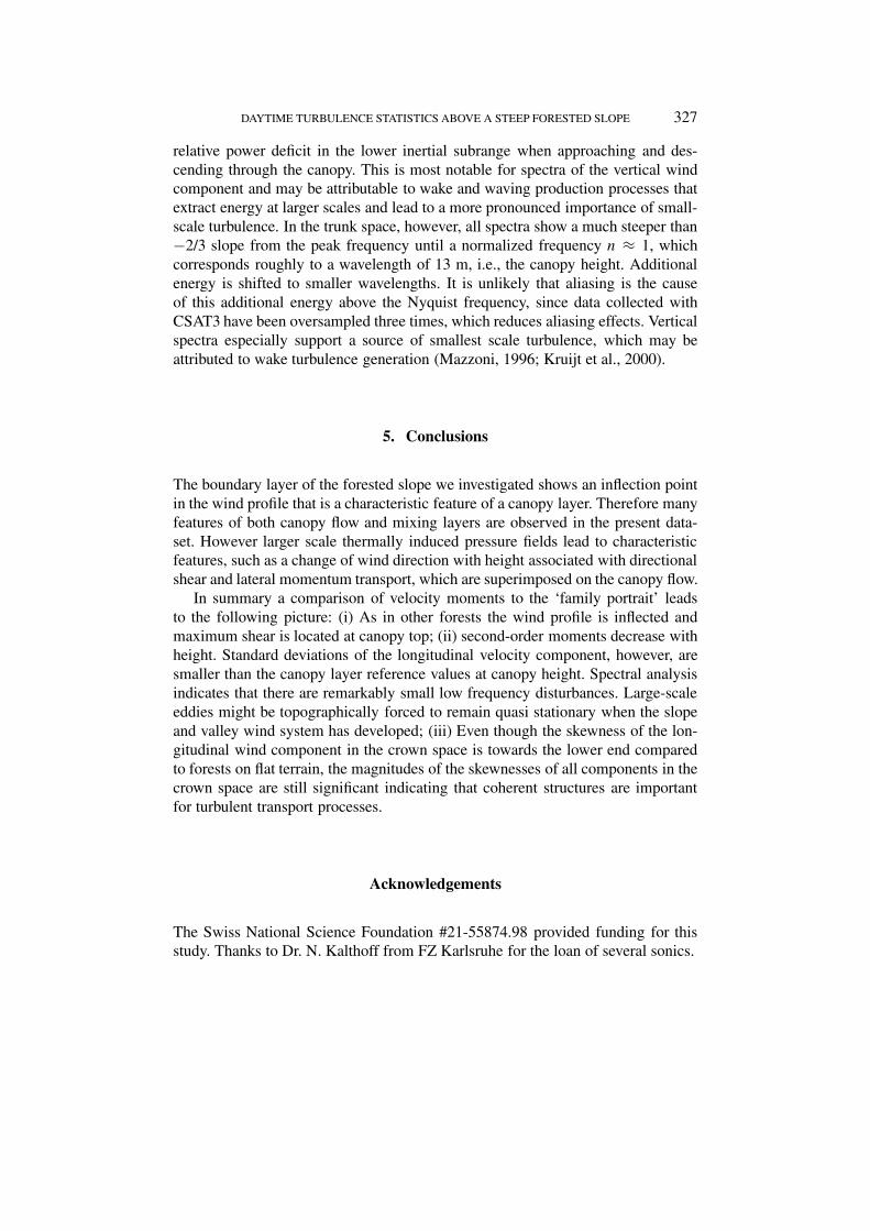
DAYTIME TURBULENCE STATISTICS ABOVE A STEEP FORESTED SLOPE 327
relative power deficit in the lower inertial subrange when approaching and des-cending through the canopy. This is most notable for spectra of the vertical windcomponent and may be attributable to wake and waving production processes thatextract energy at larger scales and lead to a more pronounced importance of small-scale turbulence. In the trunk space, however, all spectra show a much steeper than−2/3 slope from the peak frequency until a normalized frequency n ≈ 1, whichcorresponds roughly to a wavelength of 13 m, i.e., the canopy height. Additionalenergy is shifted to smaller wavelengths. It is unlikely that aliasing is the causeof this additional energy above the Nyquist frequency, since data collected withCSAT3 have been oversampled three times, which reduces aliasing effects. Verticalspectra especially support a source of smallest scale turbulence, which may beattributed to wake turbulence generation (Mazzoni, 1996; Kruijt et al., 2000).
5. Conclusions
The boundary layer of the forested slope we investigated shows an inflection pointin the wind profile that is a characteristic feature of a canopy layer. Therefore manyfeatures of both canopy flow and mixing layers are observed in the present data-set. However larger scale thermally induced pressure fields lead to characteristicfeatures, such as a change of wind direction with height associated with directionalshear and lateral momentum transport, which are superimposed on the canopy flow.
In summary a comparison of velocity moments to the ‘family portrait’ leadsto the following picture: (i) As in other forests the wind profile is inflected andmaximum shear is located at canopy top; (ii) second-order moments decrease withheight. Standard deviations of the longitudinal velocity component, however, aresmaller than the canopy layer reference values at canopy height. Spectral analysisindicates that there are remarkably small low frequency disturbances. Large-scaleeddies might be topographically forced to remain quasi stationary when the slopeand valley wind system has developed; (iii) Even though the skewness of the lon-gitudinal wind component in the crown space is towards the lower end comparedto forests on flat terrain, the magnitudes of the skewnesses of all components in thecrown space are still significant indicating that coherent structures are importantfor turbulent transport processes.
Acknowledgements
The Swiss National Science Foundation #21-55874.98 provided funding for thisstudy. Thanks to Dr. N. Kalthoff from FZ Karlsruhe for the loan of several sonics.

328 E. VAN GORSEL ET AL.
References
Barry, R. G.: 1992, Mountain Weather & Climate, 2nd edn., Routledge, London and New York, 402pp.
Christen, A., van Gorsel, E., Andretta, M., Calanca, P., Rotach, M. W., and Vogt, R.: 2000, ‘Inter-comparison of Ultrasonic Anemometers during the MAP-Riviera Project’, in Ninth Conferenceon Mountain Meteorology, Aspen, CO, August 7–11, 2000, American Meteorological Society,45 Beacon St., Boston, MA, pp. 130–131.
Christen, A., van Gorsel, E., Vogt, R., Andretta, M., and Rotach, M. W.: 2001, ‘Ultrasonic An-emometer Instrumentation at Steep Slopes: Wind Tunnel Study – Field Intercomparison –Measurements’, in MAP Meeting Schliersee, in MAP Newsletter 15, May 14–16, pp. 206–209.
De Bruin, H. A. R., Kohsiek, W., and van den Hurk, B. J. J. M.: 1993, ‘A Verification of SomeMethods to Determine the Fluxes of Momentum, Sensible Heat, and Water Vapour using Stand-ard Deviation and Structure Parameter of Scalar Meteorological Quantities’, Boundary-LayerMeteorol. 63, 231–257.
Egger, J.: 1990, ‘Thermally Forced Flows: Theory’, in W. Blumen (ed.), Atmospheric Processes overComplex Terrain, 23, American Meteorological Society, Boston, MA, pp. 43–57.
Finnigan, J.: 2000, ‘Turbulence in Plant Canopies’, Annu. Rev. Fluid Mech. 32, 519–571.Finnigan, J. J. and Brunet, Y.: 1995, ‘Turbulent Airflow in Forests on Flat and Hilly Terrain’, in M. P.
Coutts and J. Grace (eds.), Wind and Trees, Cambridge Universtiy Press, Cambridge, pp. 3–40.Kaimal, J. C.: 1978, ‘Horizontal Velocity Spectra in an Unstable Surface Layer’, J. Atmos. Sci. 35,
18–24.Kaimal, J. C. and Finnigan, J. J.: 1994, Atmospheric Boundary Layer Flows, Oxford University Press,
Oxford, 289 pp.Kruijt, B., Malhi, Y., Lloyd, J., Nobre, A. D., Miranda, A. C., and Pereira, M. G. P.: 2000, ‘Turbulence
Statistics above and within Two Amazon Rain Forest Canopies’, Boundary-Layer Meteorol. 94,297–331.
Maitani, T. and Shaw, R. H.: 1990, ‘Joint Probability Analysis of Momentum and Heat Fluxes at aDeciduous Forest’, Boundary-Layer Meteorol. 52, 283–300.
Mazzoni, R.: 1996, Turbulenzstruktur im gestörten Nachlauf einer künstlichen Oberflächenmodifika-tion. Ein Feldexperiment, Ph.D. Dissertation, ETH Zürich, Zürich, 133 pp.
Panofsky, H. A. and Dutton, J. A.: 1984, Atmospheric Turbulence – Models and Methods forEngineering Applications, J. Wiley, New York, 397 pp.
Peltier, L. J., Wyngaard, J. C., Khanna, S., and Brasseur, J.: 1996, ‘Spectra in the Unstable SurfaceLayer’, J. Atmos. Sci. 53, 49–61.
Rannik, Ü. and Vesala, T.: 1999, ‘Autoregressive Filtering versus Linear Detrending in Estimation ofFluxes by the Eddy Covariance Method’, Boundary-Layer Meteorol. 91, 259–280.
Raupach, M. R.: 1988, ‘Canopy Transport Processes’, in W. L. Steffen and O. T. Denmead (eds.),Flow and Transport in the Natural Environment: Advances and Applications, Springer, Berlin,pp. 95–127.
Raupach, M. R. and Finnigan, J. J.: 1997, ‘The Influence of Topography on Meteorological Variablesand Surface-Atmosphere Interactions’, J. Hydrol. 190, 182–213.
Raupach, M. R. and Thom, A. S.: 1981, ‘Turbulence in and above Plant Canopies’, Annu. Rev. FluidMech. 13, 97–129.
Raupach, M. R., Finnigan, J. J., and Brunet, Y.: 1996, ‘Coherent Eddies and Turbulence in VegetationCanopies: The Mixing-Layer Analogy’, Boundary-Layer Meteorol. 78, 351–382.
Rotach, M. W., Calanca, C., Vogt, R., Steyn, D. G., Graziani, G., and Gurtz, J.: 2000, ‘The TurbulenceStructure and Exchange Processes in an Alpine Valley: The MAP-Riviera Project’, in Ninth Con-ference on Mountain Meteorology, Aspen, CO, August 7–11, American Meteorological Society,45 Beacon St., Boston, MA, pp. 231–234.

DAYTIME TURBULENCE STATISTICS ABOVE A STEEP FORESTED SLOPE 329
Shaw, R. H., Brunet, Y., Finnigan, J. J., and Raupach, M. R.: 1995, ‘A Wind Tunnel Study of AirFlow in Waving Wheat: Two Point Velocity Statistics’, Boundary-Layer Meteorol. 76, 349–376.
Shaw, R. H., Tavangar, J., and Ward, D. P.: 1983, ‘Structure of the Reynolds Stress in a CanopyLayer’, J. Clim. Appl. Meteorol. 22, 1922–1931.
Vogt, R.: 1995, Theorie, Technik und Analyse der experimentellen Flussbestimmung am Beispiel desHartheimer Kiefernwaldes, Ph.D. Dissertation, University of Basel, Basel, 101 pp.
Whiteman, C. D.: 1990, ‘Observations of Thermally Developed Wind Systems in MountinousTerrain’, in W. Blumen (ed.), Atmospheric Processes over Complex Terrain, 23, AmericanMeteorological Society, Boston, MA, pp. 5–42.
Whiteman, C. D. and Allwine, K. J.: 1989, ‘Deep Valley Radiation and Surface Energy BudgetMicroclimates. Part I: Radiation’, J. Appl. Meteorol. 28, 414–426.
Wood, N.: 2000, ‘Windflow over Complex Terrain: A Historical Perspective and the Prospect forLarge-Eddy Modelling’, Boundary-Layer Meteorol. 96, 11–32.

Copyright © 2022 FDOKUMEN