DISCRETE AND CONTINUOUS Website: www.aimSciences.orgDYNAMICAL SYSTEMSSupplement 2009 pp. 404–415

INTELLIGENT TRAFFIC CONTROL ON INTERNET-LIKE

TOPOLOGIES - INTEGRATION OF GRAPH PRINCIPLES TO

THE CLASSIC RUNGE–KUTTA METHOD

Antonia Katzouraki

Electrical & Electronic Engineering, Imperial College London, UK

Tania Stathaki

Electrical & Electronic Engineering, Imperial College LondonSW7 2AZ, UK

Abstract. ‘No man is an island’ [John Donne]. Human and technological net-works play a vital part in our lives, and their failures have often caused severeadverse consequences. In this paper we address this crucial issue by presentinga model to prevent not only network failures but also their propagation to theremaining network elements. Our model forecasts the number of packets eachnode is able to service without becoming overloaded, by determining the tran-sition probabilities assigned to each link. Thus, our model ensures that nodesreceive as many packets as their network resources prescribe. The model isportable to any type of topology and is based on Ordinary Differential Equa-tions (ODEs), which are numerically solved as a multivariable, coupled system,over a variety of topologies. Our numerical algorithm is based on the classicRunge–Kutta 4th order, which is adjusted to integrate graph principles.

1. Introduction. Real world events have shown that network load can be affected,either due to a physical catastrophe or unexpected increase of the number of clientsrequesting service. A characteristic example is that of the 10th of August 1996,when a voltage-based failure occurred in two power lines. Major power distur-bances were propagated through a series of cascading failures, ultimately leading toblackouts in 11 US states and 2 Canadian provinces, leaving 7 million people with-out power for up to 16 hours [20]. In such cases, a network provider must be ableto quickly dynamically balance the load (network’s demand and supply) accordingto the available network resources and prevent a cascading failure.

To date there have been continuous advances in Internet research along with itsconnectivity structures [1]. In particular, recently there has been much interest instudying cascading failures in complex networks. Initially Motter and Lai suggesteda capacity model (ML) to describe cascade failures [15]. According to this model,the capacity is assigned in proportion to the load. Later, an analytical calculationof the capacity parameter was investigated [21]. Additionally, a costless strategyof defence was introduced and investigated to control and reduce the size of thecascade failures [14]. Recently, an improvement of the existing ML capacity modelwas suggested, in which the model is further generalized so that the proportionality

2000 Mathematics Subject Classification. Primary: 58F15, 58F17; Secondary: 53C35.Key words and phrases. Ordinary Differential Equations, Equilibrium Model.The authors are supported by DTC grant.

404

INTELLIGENT TRAFFIC CONTROL 405

constant is now changed to an increasing function of load [19]. In other research,excitable networks have been modeled by Hodgkin–Huxley [12], Bonhoeffer–vander Pol-FitzHugh–Nagumo (BPFN) [4, 3] and Kuramoto oscillators [16, 17], toinvestigate performance in terms of activity and the subsequent synchronizationof the coupled excitable elements. In a recent work, the performance of BPFNoscillators coupled on Small–World networks [8] was investigated to find that thereis no simple dependence on the network topology, instead, it is affected by thecomplex pattern of interactions throughout the entire network [18]. Furtheremore,Frank Kelly derived a mathematical model based on ODEs to analyze the stabilityand fairness of a simple rate control algorithm defining a dynamical system [10, 11].D’apice et al investigate a macroscopic fluid model on telecommunication networkswith sources and destinations [2], whereas Marigo investigates equilibrium solutionsfor data flows on networks [13].

In this paper we present a capacity model, to balance network load accordingto the available resources. A set of ODEs relates the capacity to the load. Ourmodel finds the best possible operating points for both traffic within each node andtransition probabilities assigned to each link. In particular, we assign two ODEsto each network node to describe the change of both the number of packets withineach node and the transition probabilities assigned to each link (the probability thata packet will travel across the link). Therefore, the number of ODEs we need tonumerically solve is at least twice the size of our network. The numerical solutionprovides the number of packets each node is able to comfortably accommodate andwe call this the equilibrium point; the point at which the load is balanced amongstthe nodes. We find that network elements are exchanging packets in both a coherentand synchronized fashion according to their primitive (network resources) charac-teristics and their connectivity within the network. We experimentally find therelation between the network resources, such as buffer capacity and service abilityand the equilibrium point that each node achieves. It is vital to properly assign net-work resources without wasting them, in order to design practical stable networks.Through these findings we aim to detect network failures and automatically seekthe equilibrium points, which have a central role in preventing cascading networkfailures. In this paper we explain our numerical algorithm through which we inte-grate graph principles (network’s connectivity) to classic Runge–Kutta 4th order,in order to synchronize the coupled network elements and relate network resourcesto each node’s equilibrium point.

2. The Model’s Formulation. In the following paragraphs, we outline our modeland the parameters that it depends on, along with the probabilistic and determin-istic elements from which it is built. Consider single nodes i = 1, 2, · · · , N andlet G(V , E) be a finite directed graph, where V is the set of network nodes andE ⊆ V × V , the set of unidirectional links. Let A = [aij ] be an ad-hoc adjacencymatrix, which is completely specified by an N × N matrix. It consists of zeros andones, such that each entry aij = 1 represents a connection between the nodes i

and j, whereas 0 implies there is no connection between the respective nodes. Theadjacency matrix is continuously updated, so that network connectivity is changed.

The main parameters of our model are illustrated in Table 1. In particular, aset of N variables, x1, x2, ..., xN describe the traffic (node occupation e.g. bytes).Consider m the number of incoming links towards a single node i ∈ V . A set of

406 ANTONIA KATZOURAKI AND TANIA STATHAKI

m ∈ E variables c1, c2, ..., cm describe the cost on the m ∈ E incoming unidirec-tional links. Both the traffic, xj , and link–cost, cij parameters depend on time.Each node and link have a number of initial–packets [xi]

0 and [cij ]0 respectively,

given for the time-step tn = 0. A set of m ∈ E variables λ1, λ2, · · · , λm determinethe fraction of traffic relayed through m unidirectional links, which constitute thecoupling elements of our model. In this way the coupled network elements (linksand nodes) are synchronized through these time dependent transition probabilities,λi, ∀ i ∈ [1, · · · , m]. These probabilities ensure that nodes receive as many pack-ets as they can comfortably process. Thus transition probabilities toward almostoverloaded nodes are decreased towards zero, to correspondingly decrease the loadof the almost overloaded node. Every node is assigned a service power, si ∀ i ∈V , which describes the ability each node has to process packets. The buffer capac-ity variable, bi, ∀i ∈ V describes the maximum number of packets, within a node.Both the buffer capacity and service power parameters are independent of time.These built-in features allocated to each node operate as control parameters sincetheir values affect both the solution curves and equilibrium point. In particularthrough the term si · (1 − xi

bi) in the traffic Equation (2), which is introduced in

a following paragraph both the buffer capacity and service power determine thepool from which packet rates take their values. A node without outgoing links(i, j) ∈ E should not attract more packets, and thus its service power should even-tually become zero. With regard to the probability distribution of traffic arrivingat a particular incoming link (i, j) ∈ E , the following two conditions must hold: (I)The total mass of its elements is unity. (II) The probability of traffic arriving atan incoming link is inversely proportional to its current traffic load. The secondcondition on the transition probabilities ensures that each of the network elementsis neither idle nor overloaded. Thus, transition probabilities follow the principlethat the higher the cost, the fewer packets are sent through the link. This is mathe-matically implemented by setting each transition probability inversely proportionalto the respective link cost. The transition probability for each link is denoted as anelement of the N ×N matrix, Λ = [λij ], which is defined such that λij ∈ [0, 1] with:

λij :=∑

j∈V

λij = 1, ∀i ∈ V , and is determined by the relation,

λij =

1cij

∑

k∈V

[

1

cik

] , ∀ (i, j) ∈ E such that cik 6= 0 ∀ k ∈ V . (1)

The aforementioned relation not only depends upon time t, but also on bothcost, cij , ∀ link (i, j) ∈ E and node occupation (traffic), xi, ∀ i ∈ V . This is becausecij depends on xi, through the following Equations (2) and (3). The non–negativereal–valued traffic variable, xj ∈ ℜ+∗, ∀ node j ∈ V , describes the change in thenumber of packets within each node j ∈ V . The traffic rate is given by

dxj

dt=

N∑

i=1

λijsixi

(

1 −xi

bi

)

− sjxj

(

1 −xj

bj

)

. (2)

Through the non–negative link–cost variable, cij ∈ ℜ+∗ ∀ link (i, j) ∈ E , wecalculate the number of packets that occupy each link, (i, j) ∈ E . Each link–costvariable is modeled by a nonlinear function, in order to deliver the least possible

INTELLIGENT TRAFFIC CONTROL 407

(a) (b)

Figure 1. (a). Illustration of a 2–node graph and (b). a 25–nodeRavsz-Barabasi graph.

congested service. The link–cost rate is given by

dcij

dt= λij ·

[

si · (xj)2

(1 + (xj)2)−

sj · (xi)2

(1 + (xi)2)

]

, (3)

and describes the cost ∀ incoming link (i, j) ∈ E , that is transferring traffic fromnode i ∈ V to node j ∈ V .

Table 1. Model’s Parameters

Time dependent parameters Control parameters(independent of time)

Number of packets within node i: xi ∀i ∈ V Buffer capacity for node i: bi, i ∈ V

Traffic — 1 × N matrix 1 × N matrix

Number of packets within link (i, j): cij ∀(i, j) ∈ E Power ability of node i: si, i ∈ V

Link–cost — N × N matrix 1 × N matrix

Transition Probability — Coupling elementΛ = [λij ],∀(i, j) ∈ E: N × N matrix

The concept behind the introduced link-cost function is that ‘Internet tracescome into bursts of bytes’ [6], whilst in social networks ‘people bring more people’.This is mathematically described by the sigmoid curve. This ensures the networkresponds rapidly to large influxes of packets, without overreacting to small changesin activity. In the link-cost function described in Equation (3), small increases oftraffic cause a very small increase in the cost (few people/bytes would not changethe cost), whereas slightly higher volumes of traffic (large crowd of people/burst ofbytes) would initiate a more dramatic increase in cost, in order to accommodatethe number of people/bytes.

3. Integrating Graph Principles to Classic Runge–Kutta method. Here,the traffic and link–cost ODEs (2) and (3), are coupled to lead to a large systemand further generalized through their application to multiple nodes. We modify theclassic Runge–Kutta method to include network connectivity and synchronise the

408 ANTONIA KATZOURAKI AND TANIA STATHAKI

coupled network elements (nodes and links). An implicit solution is more efficient,but also computationally more expensive as it evaluates more functions per timestep. We consider it to be beyond the scope of this paper to apply an implicitmethod. Instead, an explicit solution for xn+1 and cn+1 in terms of known valuesat tn is provided. The application of a lower order method, such as Euler or itsimproved version, also known as Runge-Kutta second order, would be less accuratecompared with Runge-Kutta forth order. A more accurate approximation, throughthe application of Euler, would require the decrease of the time step. This decreasewould increase the amount of steps required to reach the desired accuracy. Fur-thermore, short step sizes may lead to an accumulation of errors due to arithmetictruncation error through finite precision arithmetic. In the introduced algorithm weapply Runge-Kutta forth order and the time step is of the size 102. The introducedalgorithm provides the same accuracy in results with the smaller time step, such as106, but without the cost of taking increased time and using more computationalpower.

Our model is applied to directed graphs with bidirectional links. However,throughout the numerical analysis we choose the cheapest direction on each link,which is capable of transferring more traffic and has the least potential to createlink–bottlenecks during the traffic distribution on the graph G(V , E). For example,for the case of a link (i, j) through which we transfer packets either from node i toj or node j to i, we choose the cheapest direction. Thus, node i either forwardspackets to node j or receives packets from node j but not both. After preventingbottlenecks within links, we search for nodes without service power to prevent bot-tlenecks within nodes. A node i ∈ V without outgoing links is either deactivateddue to malfunction or has no available service power for new packets. Thus, inorder to stop this node from receiving more packets we set service power [si], i ∈ Vto zero. Our model relates the buffer capacity and service power of each node as aform of the traffic load (number of packets). It is applied to a static network (withrespect to the number of packets injected), in which nodes start exchanging packetsuntil they reach equilibrium. Without loss of generality, this version of our modellacks sink (more incoming flow) and source (more outgoing flow) nodes.

We simultaneously numerically solve the coupled traffic and link–cost differentialequations. Restrictions are set on the time dependent (traffic and link–cost) vari-ables, to ensure non–negative values for both the traffic and link–cost variables. Wethen calculate the current number of incoming links (m) for each node, to find thenumber of coupled ODEs that describe the state of the studied node. In particular,the number of ODEs required to be solved is at least twice the size of our network.In other words, it is m link-cost equations and one traffic equation, through whichthe state of a single node is described. This large system is numerically solvedthrough the classic Runge-Kutta formula i.e. explicit form of the 4th order [7],which is adjusted in order to include the transition probability matrix [λij ]. Thus,after the calculation of each traffic and link-cost slope approximation we readjustthe link-cost values and recalculate the transition probabilities to ensure transfer ofthe appropriate quantity of packets in the most desirable direction.

In the following section, we present numerical solutions from both the originalversion of the introduced Dynamically Adjusted Traffic Rate Alterations (DATRA)model [9] and its second version, DATRAv2, which is presented in this paper. Thesignificant difference is that however dynamics are described by the same set ofODEs, those ODEs are solved as two single variable problems in the first version,

INTELLIGENT TRAFFIC CONTROL 409

whereas in the second one as one multivariable problem. According to the firstversion of the introduced model, Runge-Kutta is deployed to solve the traffic ODEwhile the link cost is always inversely proportional to the traffic. Furthermore,Runge–Kutta is deployed for second time in order to solve the link–cost ODE. Thusin the first version of the introduced model traffic and link cost ODEs are solvedas two single–variable problems, whereas in the second version are solved as onemultivariable problem.

According to the first version of the introduced algorithm, the first single–variableproblem is summarised through the following recursion formulas:

cnij =

1

xnj

,

λnij =

1

cnij

,∑

λnij = 1,

cn+1ij = cn

ij + h,

xn+1j = xn

j +1

6· (sn

1 + 2 · sn2 + 2 · sn

3 + sn4 ),

whereas the second single–variable problem is summarised through the followingrecursion formulas:

xn+1j = xn

j + h,

cn+1ij = cn

ij +1

6· (kn

1 + 2 · kn2 + 2 · kn

3 + kn4 ) .

According to the second version, the model is solved as one multivariable prob-lem, which is described by the following recursion formulas:

xn+1j = xn

j + h/6 · (sn1 + 2 · sn

2 + 2 · sn3 + sn

4 ),

λn+1ij =

1

cnij

,∑

λn+1ij = 1,

cn+1ij = cn

ij + h/6 · (kn1 + 2 · kn

2 + 2 · kn3 + kn

4 ),

In the following sections without loss of generality and for reasons of simplicity,we illustrate numerical results from our model applied to graphs of two nodes,Figure 1.a and the well known Ravsz–Barabasi graph of twenty–five nodes [5] inFigure 1.b. We analyze the experimental results to demonstrate that: (I) Thenumber of equilibrium–packets at each node depends on every node’s buffer capacityand service power; (II) Both the solution curves and the equilibrium points aresynchronized due to the coupling element between nodes which depends on theirconnectivity; (III) The nature of the solution curves depends on both the buffercapacity and the service power assigned to each node.

4. Numerical Results for a 2–Node Graph, G(2, 2). Consider the simplestgraph G(2, 2) depicted in Figure 1.a, that consists of two nodes and two unidirec-tional links. We apply DATRAv2 to illustrate the behaviour of the traffic and its

410 ANTONIA KATZOURAKI AND TANIA STATHAKI

0 20 40 60 80 1000

50

100

150

200

250

300

Time (secs)

Num

ber

of P

acke

tsDATRAv1

node 1node 2

(a)

0 0.5 1 1.5 2 2.5 3 3.5 40

50

100

150

200

250

300

Time Steps

Num

ber

of P

acke

ts

DATRAv2 − 2 nodes graph

Sim 1Sim 1Sim 2Sim 2Sim 3Sim 3Sim 4Sim 4

(b)

Figure 2. (a) DATRAv1 model applied to a 2–node graph —solution curves for each node separately. (b) DATRAv2 runs on a2–node graph G(2, 4). Five pairs of data solutions are illustrated.

rate over time for each node i ∈ G(2, 2). The control parameters are listed as fol-lows. Link–cost capacities: [c11]

0 = 0, [c12]0 = 250, [c21]

0 = 50, [c22]0 = 0. Number

of initial packets [x1]0 = 250, [x2]

0 = 50. Each time we numerically solve our model,we vary the control parameters accordingly to reach different equilibrium points. InFigure 2.b, we present four pairs of the numerical solutions of the Equations (2) and(3) applied to the graph G(2, 2). We explain which control parameter is changedfor each example, in order for each node to reach a different equilibrium point.

For the first two examples we keep the same network characteristics, only chang-ing the buffer capacities. For the first example we set buffer capacities [bi] =[350, 350] and service power, [si] = [10, 10], equal for each node i ∈ G. The numer-ical results for this example are illustrated by the dotted lines in Figure 2.b. Weobserve that both nodes reach the same equilibrium point, at which they maintainthe same number of equilibrium–packets. In the second example we set differentbuffer capacities for each node, [bi] = [550, 350]. Results from this example are illus-trated by the solid lines in Figure 2.b. Each of these solid curves reaches differentequilibrium points, which are inversely proportional to their buffer capacity.

In the third example dash-dot lines illustrate numerical results, through which weobserve that by increasing the service power to [si] = [30, 30] the system reaches thesame equilibrium point as the dotted solution curves, but this time more quickly.In the last example buffer capacities are set to be the same, whereas the servicerates are unequal, [si] = [40, 10]. This time (dashed solution curves) we observe asignificantly faster response time with introduced overshoot, which is triggered bythe difference between each node’s service power. In Figure 2.b we observe thataccording to the dashed lines the number of packets within node 1 is dramaticallydecreased, jumping from 250 packets to 100 packets within the first 0.25 seconds.

Application of the original version of our numerical algorithm [9]. Inthis example we consider the same graph, G(2, 2) with homogeneously distributedcontrol parameters, similar with the example in Section 4. We provide experimentalevidence that DATRAv2 achieves equilibrium 100 times more quickly than theoriginal DATRAv1 algorithm. In Figure 2.a, solution curves for nodes one andtwo are produced by our original model DATRAv1, symmetrically oscillate around

INTELLIGENT TRAFFIC CONTROL 411

0 50 100 150 20050

100

150

200

250

Time Steps

Num

ber

of P

acke

ts

Ravsz−Barabasi graph with 25 nodes

(a)

0 50 100 150 20050

55

60

65

70

75

80

85SubGraph 3

Time Steps

Num

ber

of P

acke

ts

(b)

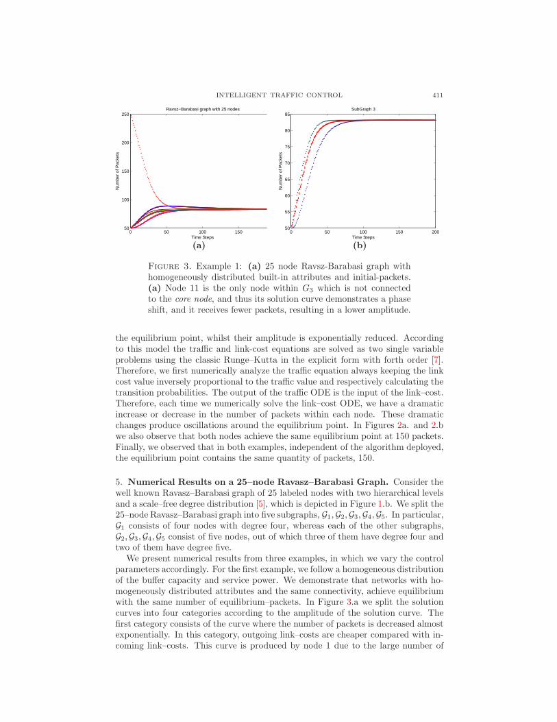
Figure 3. Example 1: (a) 25 node Ravsz-Barabasi graph withhomogeneously distributed built-in attributes and initial-packets.(a) Node 11 is the only node within G3 which is not connectedto the core node, and thus its solution curve demonstrates a phaseshift, and it receives fewer packets, resulting in a lower amplitude.

the equilibrium point, whilst their amplitude is exponentially reduced. Accordingto this model the traffic and link-cost equations are solved as two single variableproblems using the classic Runge–Kutta in the explicit form with forth order [7].Therefore, we first numerically analyze the traffic equation always keeping the linkcost value inversely proportional to the traffic value and respectively calculating thetransition probabilities. The output of the traffic ODE is the input of the link–cost.Therefore, each time we numerically solve the link–cost ODE, we have a dramaticincrease or decrease in the number of packets within each node. These dramaticchanges produce oscillations around the equilibrium point. In Figures 2a. and 2.bwe also observe that both nodes achieve the same equilibrium point at 150 packets.Finally, we observed that in both examples, independent of the algorithm deployed,the equilibrium point contains the same quantity of packets, 150.

5. Numerical Results on a 25–node Ravasz–Barabasi Graph. Consider thewell known Ravasz–Barabasi graph of 25 labeled nodes with two hierarchical levelsand a scale–free degree distribution [5], which is depicted in Figure 1.b. We split the25–node Ravasz–Barabasi graph into five subgraphs, G1,G2,G3,G4,G5. In particular,G1 consists of four nodes with degree four, whereas each of the other subgraphs,G2,G3,G4,G5 consist of five nodes, out of which three of them have degree four andtwo of them have degree five.

We present numerical results from three examples, in which we vary the controlparameters accordingly. For the first example, we follow a homogeneous distributionof the buffer capacity and service power. We demonstrate that networks with ho-mogeneously distributed attributes and the same connectivity, achieve equilibriumwith the same number of equilibrium–packets. In Figure 3.a we split the solutioncurves into four categories according to the amplitude of the solution curve. Thefirst category consists of the curve where the number of packets is decreased almostexponentially. In this category, outgoing link–costs are cheaper compared with in-coming link–costs. This curve is produced by node 1 due to the large number of

412 ANTONIA KATZOURAKI AND TANIA STATHAKI

0 50 100 150 20050

55

60

65

70

75

80

85SubGraph 2

Time Steps

Num

ber

of P

acke

ts

node 6node 7node 8node 9node 10

(a)

0 50 100 150 20050

55

60

65

70

75

80

85

Time Step

Num

ber

of P

acke

ts

SubGraph 5

node 21node 22node 23node 24node 25

(b)

Figure 4. Example 2: Ravsz-Barabasi graph, G2, G5: non-homogeneously distributed buffer capacities.

initial–packets. The second category consists of the solutions, which are producedby G1. As this graph consists of four homogeneous nodes (same connectivity andcontrol parameters) their curves are also homogeneous. We observe that the G1

subgraph receives a larger number of packets compared with G2, G3, G4 and G5.This larger amount of traffic is created due to the fact that G1 has better con-nectivity with node 1, as all nodes ∈ G1 are connected directly to node 1. Thethird category consists of curves for nodes ∈ {G2,G3,G3,G5}, which are connectedto node 1. The final category consists of solutions that oscillate with the minimumamplitude. These solution curves are produced from nodes ∈ {G2,G3,G3,G5} whichare not connected to node 1. In Figure 3.b curves from nodes that belong to thesecond subgraph G2 are illustrated. Node 6 is the only node within G2, which isnot connected to node 1. Its curve demonstrates a phase shift, as it receives fewerpackets.

In the second example we distribute the buffer capacities of each node in a non–homogeneous fashion. Through this simulation we present the relationship betweenthe buffer capacity and the equilibrium that each node achieves. The higher thebuffer capacity assigned, the lower the equilibrium point achieved. As a result of thenon–homogeneous distribution of the buffer capacities, each of the nodes achieves adifferent equilibrium, which depends on its buffer capacity. Figure 4.a demonstratesthe solution curves for each of the nodes that belong to the second subgraph, G2.Nodes labeled 8 and 10 are assigned larger buffer capacities — [b8] = 650, [b10] =400 — to achieve equilibrium with smaller number of packets, compared with theequilibrium that the other three nodes achieve, within G2. We also observe thatnode 8 achieves equilibrium with fewer packets (as its buffer capacity is [b8] = 650> [b10] = 400) compared with the equilibrium–packets for node 10. For the samereason, node 8 is assigned a larger buffer capacity ([b8] = 650 > [b1] = 560) thannode 1, and thus the number of equilibrium–packets for node 8 is less than for node1. Figure 4.b shows the synchronised solution curves for the nodes that belong tothe fifth subgraph, G5. Node 22 is assigned a relatively large buffer capacity ([b22]= 450) and therefore is the one that achieves the equilibrium point with the leastnumber of equilibrium–packets compared with the rest of the nodes ∈ G5.

INTELLIGENT TRAFFIC CONTROL 413

0 50 100 150 20030

40

50

60

70

80

90

100SubGraph 4

Time Steps

Num

ber

of P

acke

ts

node 16node 17node 18node 19node 20

(a)

0 50 100 150 20020

30

40

50

60

70

80

90

100

110SubGraph 5

Time Steps

Num

ber

of P

acke

ts

node 21node 22node 23node 24node 25

(b)

Figure 5. Example 3: G4, G5: Ravsz-Barabasi graph with non-homogeneously distributed buffer capacities and service powers

Finally, we illustrate results from the third example, according to which all the at-tributes characterising each node are distributed in a non–homogeneous way. Figure5 illustrates solution curves produced from nodes that belong to G4 and G5. Thisexample shows that regardless of the non–homogeneity of the graph’s attributes,the curves are synchronised and lead to analogous equilibrium. Furthermore, nodesassigned a high service power produce overshoot for the first ten time steps, whiletheir high service power affects the number of equilibrium packets. Figure 5.a il-lustrates the solutions from the nodes that belong to the fourth subnet, G4. Node16 has no communication link with node 1 and is the only one that that is notintroducing overshoot in its curve. Node 18 is assigned twice the service power,compared with the other nodes within G4. Therefore, it only forwards packets toits first neighbours. Nodes 17, 19 and 20 have a significantly faster response timewith introduced overshoot, as they are directly connected to node 1 and node 18.Therefore, we observe in Figure 5.a that the number of packets within nodes 17, 19,and 20 is dramatically increased, jumping from 50 to 100 packets within the first 10time steps. They also achieve the same equilibrium point, as they are allocated thesame value for both their buffer capacities and service powers. Moreover, we observethat the higher service power affects the equilibrium point. Figure 5.b illustratescurves that describe the number of packets at each time step, for nodes within thefifth subgraph, G5. Nodes 21, 23 and 24 are allocated the same values for their buffercapacities and service powers, therefore they achieve the same equilibrium point.In contrast, node 22 achieves a lower equilibrium compared with the others. Node21 is not connected to node 1 and is the only one that is not introducing overshoot.Node 25 is assigned a three times stronger service power, compared with the othernodes within G5, causing a lower equilibrium point, by means of overshoot.

6. Conclusions. Through our model, we find the best possible function of thebuffer capacity and service power as a form of the traffic load (number of packets).The function is characterized as the best possible with respect to the synchroniz-

ability of solution curves. The coupling element λij comprises the optimalfeature ofour model through which we synchronize our solution curves, taking considerationboth the node properties (buffer capacity and service ability) and the network’s

414 ANTONIA KATZOURAKI AND TANIA STATHAKI

connectivity. We inject a specific number of packets and we allocate network re-sources, such as buffer capacity and service power to initialise our test network. Ourmodel fairly distributes the number of initial packets to each node and very quicklyachieves equilibrium. The coupled model DATRAv2 is better than its original ver-sion [9], as it achieves equilibrium almost hundred times more quickly, withoutoscillating around the equilibrium point. We observed the inversely proportionalrelationship between the buffer capacity and number of equilibrium—packets. Ad-ditionally, high service power nodes ‘shot out’ too many packets to their neighbours,which affected both their equilibrium and nature of the solution curves. Taking theabove points into consideration, we conclude that it is vital to properly assign net-work resources such as buffer capacity and service power, in order to design a stablenetwork (in terms of the solution curves). Our suggested model for assigning buffercapacities and service powers to nodes will be useful in designing practical stablenetworks, without wasting the resources. During a simulation (numerical analysisof an example), given that the number of initial packets injected into the networkis static, our model always reaches an equilibrium solution.

Acknowledgments. The authors would like to thank Alexandre Caboussat (De-partment of Mathematics, University of Houston) for his valuable comments andsuggestions.

REFERENCES

[1] D. Alderson, H. Chang, M. Roughan and S. Uhlig, W. Willinger The many

facets of internet topology and traffic Netw. Heterog. Media, 1, (2006), 569–600,http://www.ams.org/mathscinet-getitem?mr=2276254.

[2] C. D’Apice, R. Manzo and B. Piccoli A fluid dynamic model for telecommunication networks

with sources and destinations SIAM Journal on Applied Mathematics (2008), 68, 4, 981–1003,http://www.ams.org/mathscinet-getitem?mr=2455475.

[3] D. E. Boschi, C. and Louis, E. and Ortega, G. Triggering synchronized oscillations through

arbitrarily weak diversity in close-to-threshold excitable media Phys. Rev. E 65 1 (2001).[4] Cartwright and Julyan H. E. Emergent global oscillations in heterogeneous excitable

media: The example of pancreatic β cells Phys. Rev. E 62 1 (2000), 1149–1154http://link.aps.org/doi/10.1103/PhysRevE.62.1149.

[5] M. Chavez and D–U. Hwang and A. Amann and H. G. E. Hentschel and S. Boccaletti Synchro-

nization is Enhanced in Weighted Complex Networks Phys. Rev. Lett. 94 (2005), 218701–4http://link.aps.org/doi/10.1103/PhysRevLett.94.218701.

[6] Allen B. Downey Evidence for long–tailed distributions in the Internet SIGCOMM conferenceon Internet measurement, (2001), 149–160.

[7] E. Hairer, F.P. Norsett and G. Wanner Solving Ordinary Differential Equations I. NonstiffProblems. Springer, Berlin-Heidelberg-New York, (1987).

[8] Hong, H. and Choi, M. Y. and Kim, Beom Jun Synchronization on small-world networks

Phys. Rev. E 65 2 (2002), 026139-13 http://link.aps.org/doi/10.1103/PhysRevE.65.026139.[9] Antonia Katzouraki and Philippe De Wilde and Robert A. Ghanea Hercock Intelligent Traffic

Control on Internet-Like Topologies - DATRA - Dynamically Adjusted Traffic Rate Alter-

ations SOAS IOS Press, Frontiers in Artificial Intelligence and Applications 135 (2005).[10] F. Kelly Mathematical modelling of the Internet ICIAM in Fourth International Congress on

Industrial and Applied Mathematics (1999).[11] F. Kelly, A. K. Maulloo and D. K. H. Tan Rate control in communication networks: shadow

prices, proportional fairness and stability. J. Operational Research Society 49 (1998).[12] Lago-Fernandez, Luis F. and Huerta, Ramon and Corbacho, Fernando and Siguenza, Juan

A. Fast Response and Temporal Coherent Oscillations in Small-World Networks Phys. Rev.Lett. 84 12 (2000).

[13] A. Marigo Equilibria for data networks Netw. Heterog. Media, 2, (2007), 497–528,http://www.ams.org/mathscinet-getitem?mr=2318843.

INTELLIGENT TRAFFIC CONTROL 415

[14] Motter and Adilson E. Cascade Control and Defense in Complex Networks Phys. Rev. Lett.93 9 (2004), 098701–4 http://link.aps.org/doi/10.1103/PhysRevLett.93.098701.

[15] Motter, Adilson E. and Lai, Ying-Cheng Cascade-based attacks on complex networks Phys.Rev. E 66, 6 (2002), 065102–5 http://link.aps.org/doi/10.1103/PhysRevE.66.065102.

[16] G. Restrepo and Edward Ott and Brian R. Hunt Onset of synchroniza-

tion in large networks of coupled oscillators Physical Review E 71 3 (2005)http://link.aps.org/doi/10.1103/PhysRevE.71.036151.

[17] B. R. Trees and V. Saranathan and D. Stroud Synchronization in disordered Josephson junc-

tion arrays: Small-world connections and the Kuramoto model Physical Review E 71 1 (2005)http://link.aps.org/doi/10.1103/PhysRevE.71.016215.

[18] I. Vragovic, E. Louis and A. Diaz–Guilera Performance of excitable small-world networks of

Bonhoeffer-van der Pol-FitzHugh-Nagumo oscillators IOP Europhys. Lett. 76 (2007).[19] B. Wang and B. J. Kim A high-robustness and low-cost model for cascading failures IOP,

EPL 78,11 (2007).[20] Western Systems Coordinating Council (WSCC) Disturbance report for the Power System

Outage that occured on Western Interconnection at 1548 PAST http://www.wscc.com.[21] Zhao, Liang and Park, Kwangho and Lai, Ying-Cheng Attack vulnerability of scale-free net-

works due to cascading breakdown Phys. Rev. E,70 3 (2004).

Received July 2008; revised August 2009.

E-mail address: ak3@imperial.ac.uk

E-mail address: tania.stathaki@imperial.ac.uk