(Preprint for)

J. Alvarez and J. RojoAn improved class of generalizedRunge-Kutta methods for stiff problems.Part II: The separated system caseAppl. Math. Comput., 159 (2003), pp. 717-758

1

An improved class of generalized

Runge-Kutta methods for stiff problems.

Part II: The separated system case

Jorge Alvarez a,1 and Jesus Rojo a,1

a Departamento de Matematica Aplicada a la Ingenierıa, E.T.S. de IngenierosIndustriales, Universidad de Valladolid, E-47011 Valladolid, SpainE-mail: joralv@wmatem.eis.uva.es, jesroj@wmatem.eis.uva.es

In order to study a generalization of the explicit p-stage Runge-Kuttamethods, we introduce a new family of p-stage formulas for the numericalintegration of some special systems of ODEs that provides better orderand stability results with the same number of stages. In our recent paperentitled ’An improved class of generalized Runge-Kutta methods for stiffproblems. Part I: The scalar case’ we studied new schemes for the numer-ical integration of scalar autonomous ODEs. In this second part we willshow that it is possible to generalize our GRK-methods so that they canbe applied to some non-autonomous scalar ODEs and systems obtaininglinearly implicit A-stable and L-stable methods. These methods do notrequire Jacobian evaluations in their implementation. Some numerical ex-amples are discussed in order to show the good performance of the newschemes.

Key words: Generalized Runge-Kutta Methods, Stiff ODEs, Linear Stability,Numerical Experiments.

1 Introduction.

In our recent paper [7], first part of this work, we introduced the general formof a new class of explicit p-stage methods for the numerical integration ofscalar autonomous ODEs. In the same paper, but also in [4,2,5], examples areshown of explicit two-stage methods of order three for the numerical integra-tion of scalar autonomous ODEs, some of them being A-stable and L-stable.

1 This work was partially supported by Programa Gral. de Apoyo a Proyectosde Investigacion de la Junta de Castilla y Leon under proyect VA024/03 and byPrograma C.I.C.Y.T under proyect BFM2002-03815.

Preprint submitted to Elsevier Preprint 29 September 2003

Comparisons with Runge-Kutta methods as well as numerical experiments arealso reported.

For brevity reasons, we refer to these methods as GRK-methods (GeneralizedRunge-Kutta methods). In what follows, we make this name also extensive tothe methods for systems that we will study here.

Recently, in the Thesis of J. Alvarez [3] the GRK-methods (and the extensionof these methods to ’separated’ systems) have been introduced and studiedin a systematic way, but the language used in this work is spanish, and so, itseems necessary to make the ideas of the Thesis available in an internationaljournal. This is the main purpose of this paper.

We will study how the GRK-methods for scalar problems can be extended(with minor changes) in order to integrate more general problems. We willshow that it is possible to obtain A-stable linearly implicit formulas for somenon-autonomous scalar ODEs and systems. In [6] we presented a first two-stage third order method for separated systems of ODEs being L-stable, aswell as preliminary results using our method to integrate systems that arisewhen solving some nonlinear parabolic PDEs by the method of lines approach.

Following this line, our aim is now to generalize this method by introducingthe family of GRK-methods in order to obtain some properties that cannot beobtained from the classical explicit Runge-Kutta formulas. In fact, as we haveseen when considering the scalar version of the GRK-methods (see [7]) themost important advantage of our methods is that we can obtain higher orderwith a reduced number of function evaluations. We will obtain linearly implicitmethods of high order with important linear stability properties that cannotbe obtained with the classical explicit Runge-Kutta methods. For example, itis possible to obtain order three and L-stability with only two stages (that istwo function evaluations per integration step). This justifies the considerationof the formulas we will present here.

Our methods show also important advantages with respect to other classicalimplicit [9] and diagonally implicit [1] Runge-Kutta methods, and Rosenbrocktype methods such as the ROW-methods (also called Rosenbrock-Wannermethods and modified Rosenbrock methods) [14,15,17] for which the exactJacobian matrix must be evaluated at each step, because for our formulas theexact Jacobian matrix must not be computed when the methods are imple-mented.

Note at this point that, as we have remarked in [2], it is also possible toobtain two-stage third order formulas (belonging to the family of methods wewill introduce) from any prefixed linear stability function. This can be of greatinterest when considering perturbed problems for which the exact solution ofthe unperturbed problem is known, because we can obtain methods specifically

2

designed to integrate exactly the unperturbed problem.

As is well known, non autonomous systems can be easily formulated as au-tonomous systems, and so our treatment will consider only the autonomouscase.

In the system case, that we are going to study here, we have that term sconsidered in [7] for the scalar case cannot be defined exactly in the sameway because now the stages k1 and k2 are vectors. So, when considering thisproblem, we will see that the formula in [7] that gives us term s, must bemodified into a formula that gives us term s as a square matrix with the samedimension of the system. Division by the vector k1 has only sense when thevectorial function f defining the system

y′ = f(y) (1)

is of a special type that we will call ’separated’ (and so the associated systemis a ’separated system’). For this, as we will see later, function f must begiven in the form (2). The special form of function f makes no availablethe GRK-methods for general systems. This limitation of the new methodsis compensated by the important advantages of our methods (higher order,better linear stability properties, ...) when applied to the class of separatedproblems, with respect to classical methods such as Runge-Kutta formulas.

We have explored some important problems of practical interest for which ourmethods can be applied. As a result of this study, we have concluded thatmany important problems of interest that are formulated in terms of ODEs orPDEs can be solved with the formulas we will propose here. We also note thatsome non autonomous equations can be formulated in terms of an autonomousseparated system and integrated with our methods.

When considering many important partial differential equations, and after asemi discretization (by using finite difference approximations) that transformthese problems into a system of ordinary differential equations, we obtainseparated systems for which our methods can be applied. For example, systemsof this type appear when solving some parabolic partial differential equationsby the method of lines. We will show examples of this later, by obtainingseparated systems of ODEs from the Burgers’ equation by the method of linesapproach (with finite difference approximations in the spatial derivatives).In (20) we will show examples of this, and more precisely, we will consider asin [6] the problem studied in [11] (pp. 349–443) involving Burgers’ equation.

When we observe the cases cited as practical in the literature we see thatmany of them are problems that we can solve with our methods. We can citefor example (26) (see [20] pp. 27 and [18]) and (28) (taken from [16], pp. 213)as interesting examples of this.

3

Following these ideas for scalar equations, we have adapted our methods inorder to obtain formulas that can be applied to many second order differ-ential equations of an special type. In [8] some preliminary results involvingperturbed oscillators can be found.

As a resume, we will show clearly that the new methods can be applied to awide class of problems considered of interest in the current literature. Also,for these problems for which the explicit (or linearly implicit) methods canbe applied, we get very high orders of convergence and specially good linearstability properties for stiff problems that completely justifies the introductionof the new schemes and its study.

Now we can begin the description of the new formulas for separated systems.

2 The problem.

We will begin considering separated systems given by

y′(1) = f11(y(1)) + f12(y(2)) + . . . + f1m(y(m)) ,

y′(2) = f21(y(1)) + f22(y(2)) + . . . + f2m(y(m)) ,

......

y′(m) = fm1(y(1)) + fm2(y(2)) + . . . + fmm(y(m)) , (2)

that is, autonomous systems of ODEs y′ = f(y) =∑m

j=1 Fj(y(j)) for whichf : IRm → IRm is given by f(y) = F (y)1l, with y = (y(1), y(2), . . . , y(m)),1l = (1, 1, . . . , 1)T and where F is the matrix

F (y) =

f11(y(1)) f12(y(2)) · · · f1m(y(m))

f21(y(1)) f22(y(2)) · · · f2m(y(m))...

......

fm1(y(1)) fm2(y(2)) · · · fmm(y(m))

, (3)

whose j-th column is given by Fj and with components fij : IR → IR. Notethat brackets are used for the components of vectors y and y′. These systemsare thus given componentwise by

y′(i) = fi(y(1), y(2), . . . , y(m)) =m∑

j=1

fij(y(j)) , 1 ≤ i ≤ m. (4)

Although the preceding expressions for the separated systems are not com-pletely determined in an unique way because the additive constants can be

4

assimilated to the components in many different ways, the methods we willintroduce later give the same result independently of where we place theseadditive constants.

Note that we begin considering only (separated) autonomous systems of ODEs,but, as we will see later, some non autonomous systems that take the formy′(x) = f(y(x)) + g(x) can be also integrated with the schemes we will in-troduce in this work. This can be easily seen by adding the trivial equationx′ = 1 to the preceding non autonomous systems so that the resulting systemtakes an autonomous form. This resulting autonomous system is one dimen-sion higher, and separated when y′(x) = f(y(x)) is separated. Our methodscan be implemented for these non autonomous problems without increasingthis dimension.

3 The new family of GRK-methods.

For problem (2), with initial condition y(x0) = y0 (y0 ∈ IRm), the general formof a p-stage method of our family is given by

yn+1 = yn + hGp+1(S2, S3, . . . , Sp) k1 , (5)

in terms of the stages

k1 = f(yn)

k2 = f(yn + hG2 k1)

k3 = f(yn + hG3(S2) k1) (6)...

kp = f(yn + hGp(S2, S3, . . . , Sp−1) k1) ,

where yn, yn+1 and the ki are m dimensional (column) vectors in IRm andwhere Si and Gi(S2, S3, . . . , Si−1) are square matrices, that is Si ∈ MIR(m)and Gi(S2, S3, . . . , Si−1) ∈ MIR(m) (MIR(m) is the space of m row squarematrices with real elements). The matrices Si take the form

f11(yn(1) + α1)− f11(yn(1))

e1 Gi(S2, S3, . . . , Si−1) k1

· · · f1m(yn(m) + αm)− f1m(yn(m))

em Gi(S2, S3, . . . , Si−1) k1...

...

fm1(yn(1) + α1)− fm1(yn(1))

e1 Gi(S2, S3, . . . , Si−1) k1

· · · fmm(yn(m) + αm)− fmm(yn(m))

em Gi(S2, S3, . . . , Si−1) k1

, (7)

where αj = h ej Gi(S2, S3, . . . , Si−1) k1 (with 1 ≤ j ≤ m) and ej is the mdimensional row vector in IRm whose components are all zero except for the

5

j-th component that takes the value 1. Note that the element in row p andcolumn q (with 1 ≤ p, q ≤ m) of the preceding matrix Si is

fpq(yn(q) + h eq Gi(S2, S3, . . . , Si−1) k1)− fpq(yn(q))

eq Gi(S2, S3, . . . , Si−1) k1

. (8)

Stages ki (1 ≤ i ≤ p) can be also given in terms of function F (see (3)) throughrelation

ki = F (yn + hGi(S2, S3, . . . , Si−1) k1)1l

=m∑

j=1

Fj(yn(j) + h ej Gi(S2, S3, . . . , Si−1) k1) , (9)

where Fj(yn(j) + h ej Gi(S2, S3, . . . , Si−1) k1) is the j-th column of the squarematrix F (yn + hGi(S2, S3, . . . , Si−1) k1) given by

f11(yn(1) + h e1 Gi(∗) k1) · · · f1m(yn(m) + h em Gi(∗) k1)...

...

fm1(yn(1) + h e1 Gi(∗) k1) · · · fmm(yn(m) + h em Gi(∗) k1)

, (10)

with (∗) denoting point (S2, S3, . . . , Sp−1), and the element in row p and col-umn q (with 1 ≤ p, q ≤ m) of this matrix given by

fpq(yn(q) + h eq Gi(S2, S3, . . . , Si−1) k1) . (11)

Now it is easily seen that the j-th column of matrices Si in (7) takes the form

Fj(yn(j) + h ej Gi(S2, S3, . . . , Si−1) k1)− Fj(yn(j))

ej Gi(S2, S3, . . . , Si−1) k1

, (12)

and is therefore given in terms of the j-th column of stage ki (see (9)) minusthe j-th column of stage k1 and divided by the term ej Gi(S2, S3, . . . , Si−1) k1

taken from the argument of the j-th column of stage ki.

From the preceding comments it is now clear that matrices Si can be seen as ageneralization (together with a minor modification) of the terms si consideredin the scalar case. In fact, it is not difficult to see that the family of methodsintroduced in [7] for scalar problems can also be formulated in this manner,but we will not do that here.

Note that matrices Si for this kind of systems can be seen as approximations tohfy(yn), that is, approximations to the Jacobian matrix of function f evaluatedin yn (and scaled by the step h). This follows from the fact that (8) can beconsidered an approximation to the partial derivative of the p-th componentof function f with respect to his q-th variable at point yn. In fact, for this kind

6

of systems we have

∂fp

∂y(q)

(yn) =∂fpq

∂y(q)

(yn(q)) ≈ fpq(yn(q) + h δq)− fpq(yn(q))

h δq

, (13)

with δq = eq Gi(S2, S3, . . . , Si−1) k1.

From our last observation we can conclude that our GRK-methods are sim-ilar to the Rosenbrock methods [19] and other related formulae such as theW-methods [22], the MROW-methods [24] and the generalized Runge-Kuttamethods [23] for which the exact Jacobian matrix must not be computed whenmethods are implemented. In [11] some of this methods can be found.

The most important advantage of our GRK-methods with respect to thesemethods is that for our formulas it is not necessary to make new evaluationsof function f to obtain the approximate Jacobian matrix. This is so becausematrices Si (from which we have the approximations to the Jacobian matrix)are obtained from the information contained in the stages ki with no extraevaluations of function f (at the only cost of working with square matricesduring the evaluations).

As we have commented before, separated systems are not completely deter-mined because of additive constants. More precisely, taking in (2) fij = fij+cij

in place of fij (1 ≤ i, j ≤ m) with cij given constants satisfying∑m

j=1 cij = 0for i = 1, 2, . . . , m , we get the same system. It is a simple task to show thatwhen we apply any of our methods to both separated systems (representingthe same system) y′ = f(y) and y′ = f(y), taking the same initial value andthe same stepsize, we obtain the same result.

4 A first two-stage GRK-method for separated systems.

Before studying in detail the new family of methods, we begin considering afirst example of a two-stage formula. Note that function G2 in (6) is constant,that is, G2 = c2I where c2 is a constant and I is the identity matrix inMIR(m). Therefore, a two-stage method for systems from the preceding familyof schemes takes the form

yn+1 = yn + hG3(S2) k1 , (14)

where the stages are

k1 = f(yn) , k2 = f(yn + hc2k1) , (15)

7

and S2 is the matrix

f11(yn(1)+hc2e1k1)−f11(yn(1))

c2e1k1

· · · f1m(yn(m)+hc2emk1)−f1m(yn(m))

c2emk1...

...

fm1(yn(1)+hc2e1k1)−fm1(yn(1))

c2e1k1

· · · fmm(yn(m)+hc2emk1)−fmm(yn(m))

c2emk1

(16)

The formula is completely determined from the values of c2 and function G3.

From Butcher’s theory we know that a Runge-Kutta method of order q forscalar problems can show order less than q when applied to systems of ODEs.However, for q ≤ 3 any Runge-Kutta method of order q for scalar autonomousproblems shows the same order when applied to systems of ODEs (see forexample [16] pp. 173-175 for more details). For our methods this result alsoholds, that is, for q ≤ 3 any GRK-method of order q for scalar autonomousproblems shows the same order when applied to separated systems of ODEs.

As a first example we will obtain an L-stable formula. In order to attain L-stability we must take G3 given by a rational function whose denominator mustbe interpreted in terms of inverse matrices (note that the argument S2 of func-tion G3 is a square matrix). We look for a function G3(s) whose denominatortakes the form (1−a s)α, that is, G3(S2) in (14) is given by (I−a S2)

−α N(S2)where α ∈ IN , a ∈ IR is a constant and N is a polynomial function (as before,I stands for the identity matrix). We take function G3 in this manner so thatonly one LU factorization must be done for each integration step. Taking thevalues α = 3, c2 = 2/3, a as the root of polynomial 6x3 − 18x2 + 9x − 1 = 0given by

a = 1 +

√6

2sin

(1

3arctan

(√2

4

))−√

2

2cos

(1

3arctan

(√2

4

))

≈ 0.435866521508459 , (17)

and function G3 in (14) given by

G3(S2) = (I − aS2)−3

(I +

1− 6a

2S2 +

1− 9a + 18a2

6S2

2

), (18)

we obtain a two-stage third order L-stable method for separated systems whoseassociated stability function takes the form

R(z) =2 + 2 (1− 3a) z + (1− 6a + 6a2) z2

2 (1− a z)3, (19)

with a given by (17).

8

For more details involving the L-stability that we get from the precedingstability function R(z), [11] pp. 96–98 is a good reference. In [6] this methodis obtained with slightly different notations.

5 A first numerical experiment with systems.

As a first example, in order to show the good performance of the preced-ing method, we will consider a numerical experiment involving the Burgers’equation

ut + uux = ν uxx or equivalently ut +

(u2

2

)

x

= ν uxx , ν > 0 , (20)

where u = u(x, t) and we take 0 ≤ x ≤ 1 and 0 ≤ t ≤ 1. Initial and Dirichletboundary conditions for our example are taken as

u(x, 0) = (sen(3πx))2 · (1− x)3/2 , u(0, t) = u(1, t) = 0 . (21)

The preceding nonlinear parabolic problem is taken from [11] (see pp. 349 and443) and was originally designed by Burgers in 1948 as a mathematical modelillustrating the theory of turbulence. Nowadays it remains interesting as anonlinear equation resembling the Navier-Stokes equations in fluid dynamics.Note that for small values of ν the solution possesses shock waves and forν → 0 we obtain discontinuous solutions. Note also that Burgers’ equation canbe considered as an example of hyperbolic problem with artificial diffusion forsmall ν.

Now we will apply the method of lines to this equation as follows. We willconsider a uniform mesh along the x-axis and replace all spatial derivatives inthe right equation of (20) by centered finite difference approximations. Taking

∆x =1

N + 1, ui(t) = u(i∆x, t) i = 0, 1, . . . , N + 1 , (22)

we get a separated system of ODEs for this method of lines approach toBurgers’ equation, that is given by

u′i = −u2i+1 − u2

i−1

4∆x+ ν

ui+1 − 2ui + ui−1

(∆x)2, i = 1, 2, . . . , N

ui(0) = (sen(3πi∆x))2 · (1− i∆x)3/2 , i = 1, 2, . . . , N , (23)

with ui = ui(t). From the boundary conditions we get that u0(t) = uN+1(t) = 0must hold. Obviously our method can be applied to the this separated system.After the appropriate exclusions and substitutions we can note by inspection

9

that the Jacobian matrix associated to this system is tridiagonal.

In [6] we have applied our method with fixed stepsize h = 0.04 to the precedingsystem taking N = 24 and ν = 0.2 and obtaining in this way the numerical so-lution (see the first figure in [6]). For these values the system becomes bandedof dimension 24 and the associated Jacobian matrix is tridiagonal. The prob-lem is mildly stiff with the eigenvalues of the Jacobian belonging to interval[−499,−1] (the dominant eigenvalue being close to −498) for the integrationinterval considered.

With fixed stepsize h = 2−k for the values k = 2, 3, . . . , 10 over 2k steps, thevalue of the numerical solution (for t = 1) was also computed in [6] by usingour method, and the magnitude of the error E (measured in the Euclideannorm of the space IR24) for the different stepsizes considered can be found inthe second figure of this work. The exact solution at the specified output pointwas computed very carefully taking fixed stepsize h = 0.0001. In the doublelogarithmic scale used for that figure, the error is closely represented by astraight line whose slope equals the order of the method. Figure shows clearlythe order three of our method, in complete agreement with our theoreticalresult.

In the following sections we will repeat this numerical experiment with otherthird and fourth order methods.

To complete this first approach to our methods for separated systems we willalso consider the following numerical experiments.

6 Some interesting numerical experiments.

We will study the family of problems taken from [13], pp. 34 (see also [21],pp. 233 and [12]).

y′1 = −(b + an)y1 + byn2 y1(0) = cn

y′2 = y1 − ay2 − yn2 y2(0) = c

(24)

whose solution is given by

y1(x) = cne−anx , y2(x) = ce−ax . (25)

We take the values a = 0.1, c = 1, n = 4 and b = 100i (i = 0, 1, 2, 3) in theinterval 0 ≤ x ≤ 10. The problem is stiffer for great values of parameter b. Infact, the eigenvalues along the exact solution satisfy λ1 ≈ −b and λ2 ≈ −a).The nonlinear character of the problems depends on the value n (the problem

10

is more nonlinear when n is great). For more details on this problem see [13].

With fixed stepsize h = 2−k for k = 0, 1, 2, . . . , 10 we integrate along 10 · 2k

steps obtaining in this way approximations to the exact solution y (for x = 10)with our two-stage method. The magnitude of the global error E (in theEuclidean norm) for the different stepsizes h and for each of the problemsconsidered is shown in Figure 1 in double logarithmic scale. It can be seenthat the method shows order less than three (in fact two) when applied to thisproblem taking b = 1000000 (marked in figure with crosses) and b = 10000(circles) for the range of stepsizes we are considering here. Taking b = 100(diamonds) the order goes from two to three when the stepsize is reduced.The order reduction can be explained in terms of the so called B-convergenceand many implicit methods also show this behaviour when applied to somenonlinear stiff ODEs. Finally, taking b = 1 (squares) the problem is no longerstiff and our method shows order three as expected.

-12

-10

-8

-6

-4

E

-3 -2 -1 0h

Fig. 1. Error as a function of the step-size in double logarithmic scale for ourmethod (autonomous problem).

PROBLEM B

PROBLEM A

-9

-7

-5

-3

-1

E

-4 -3 -2 -1 0h

Fig. 2. Error as a function of the step-size in double logarithmic scale for ourmethod (non autonomous problems).

Now we will consider two non autonomous stiff problems. Problem A is takenfrom [20], pp. 27 and is given by

y′ = −106 y + cos x + 106 sin x , y(0) = 1 , (26)

with solution

y(x) = sin x + e−106 x . (27)

11

Note that this problem can be considered as part of the family of scalar equa-tions proposed by Prothero and Robinson in [18].

Problem B is given in terms of the following non autonomous system

y′1 = −2 y1 + y2 + 2 sin x y1(0) = 2

y′2 = 998 y1 − 999 y2 + 999(cos x− sin x) y2(0) = 3(28)

taken from [16], pp. 213, for which the exact solution takes the form

y1(x) = 2e−x + sin x , y2(x) = 2e−x + cos x . (29)

Both problems are stiff (the eigenvalue for problem A is λ = −1000000 andfor problem B the eigenvalues are λ1 = −1 and λ2 = −1000). We apply ourtwo-stage method to both problems with fixed stepsizes h = 2−k for k =0, 1, 2, . . . , 11 over 10 · 2k steps. Figure 2 shows the global error E (in theEuclidean norm) as a function of the stepsize h in double logarithmic scale.As in the previous example, we can observe that the order that shows ourmethod when applied to problem A is nearly two (for the range of stepsizesconsidered here). Taking small enough stepsizes the order changes from twoto three as expected. For problem B the order changes from two to three whenthe stepsize is reduced, as can be seen in the figure. As we have pointed before,this can be explained in terms of the concept of B-convergence.

7 Order conditions for the two-stage methods.

As we have shown in the preceding numerical experiments, it is possible toobtain two-stage methods of order three for separated systems. In fact, in thiscase, the order conditions (for order three) are the same we obtained consider-ing scalar autonomous problems. In the same way as when we considered thescalar case, it suffices to obtain the order conditions for the polynomial typemethods, because from these conditions we easily obtain those of the generalformulas.

Also as in the scalar case, two-stage methods of polynomial type (for systems)can be defined as follows

yn+1 = yn + hG3(S2) k1 , (30)

where the stages are given by

k1 = f(yn) , k2 = f(yn + hc2k1) , (31)

12

S2 is the matrix

f11(yn(1)+hc2e1k1)−f11(yn(1))

c2e1k1

· · ·f1m(yn(m)+hc2emk1)−f1m(yn(m))

c2emk1...

...

fm1(yn(1)+hc2e1k1)−fm1(yn(1))

c2e1k1

· · ·fmm(yn(m)+hc2emk1)−fmm(yn(m))

c2emk1

(32)

and where function G3 is given in terms of S2 by

G3(S2) = c3

(I +

r3∑

i=1

aiSi2

), r3 ∈ IN , (33)

where I stands for the identity matrix of dimension m. Order conditions (fororder three) are the same as those given for scalar autonomous problems(see [7]), that is

c3 = 1 , (34)

c3a1 = 1/2 , (35)

c3c2a1 = 1/3 , (36)

c3a2 = 1/6 . (37)

After solving this conditions for order three, we deduce that c2 = 2/3 and thatfunction G3 associated to any third order method of polynomial type can begiven in the form

G3(S2) = I +1

2S2 +

1

6S2

2 +r3∑

i=3

aiSi2 , r3 ∈ IN , (38)

where the free parameters ai (with i ≥ 3) can be arbitrarily chosen.

Additional conditions for order four are now different from those associatedto the scalar case (see again [7]). In fact, now we have four additional orderconditions (one more than in scalar case) that are given by

c3c22a1 = 1/4 , (39)

c3c2a2 = 1/12 , (40)

c3c2a2 = 1/4 , (41)

c3a3 = 1/24 , (42)

and two of these conditions ((40) and (41)) cannot be satisfied at the sametime. It is easily seen that first three equations are not satisfied for the val-ues of the parameters that we must take so that the two-stage method hasorder three, and therefore it is not possible to obtain formulas of order fourwith only two stages (as in scalar case). However, we can satisfy the fourth

13

equation taking a3 = 1/24 in such a way that the principal part of the localtruncation error (PPLTE) is minimized. For this choice of parameter a3, andtaking also a1 = 1/2, a2 = 1/6, c2 = 2/3 and c3 = 1 (to attain order three),the resulting formulas show order four when applied to lineal problems withconstant coefficients.

Now, order conditions for two-stage methods for separated systems given interms of rational type functions, are easily obtained from those obtained forpolynomial type formulas, following the same ideas as in scalar case. A two-stage method of rational type for systems is given (generalizing the associatedmethods for scalar case) by formulas (30)–(32), where function G3 in terms ofS2 takes the form

G3(S2) = c3

I +

d∗3∑

i=1

diSi2

−1

I +n∗3∑

i=1

niSi2

, n∗3, d

∗3 ∈ IN , (43)

As in the scalar case, it suffices to take G2 = c2I with c2 = 2/3 and functionG3 given by (43) with a Taylor’s expansion in powers of S2 of the form

G3(S2) = I +1

2S2 +

1

6S2

2 + O(S32) . (44)

Therefore, it is enough to take the values n∗3 = d∗3 = 2 in (43) in order to obtainthe order conditions for order three methods of rational type from those ofpolynomial type. We easily obtain in this way the fourth order conditions

c2 = 2/3 , (45)

c3 = 1 , (46)

n1 = 1/2 + d1 , (47)

n2 = 1/6 + (1/2)d1 + d2 , (48)

as in the scalar case (see [7]).

If we also want to minimize the principal part of the local truncation error,we must take n∗3 = d∗3 = 3 in (43) and expand in (44) to one higher orderobtaining the additional condition

n3 = 1/24 + (1/6)d1 + (1/2)d2 + d3 . (49)

From the preceding considerations we deduce that the general form of a two-stage third order method of rational type for systems is

yn+1 = yn + hG3(S2) k1 , (50)

14

where stages are given by

k1 = f(yn) , k2 = f(yn +

2

3hk1

), (51)

matrix S2 takes the form

f11

(yn(1)+

23he1k1

)−f11(yn(1))

23e1k1

· · ·f1m

(yn(m)+

23hemk1

)−f1m(yn(m))

23emk1

......

fm1

(yn(1)+

23he1k1

)−fm1(yn(1))

23e1k1

· · ·fmm

(yn(m)+

23hemk1

)−fmm(yn(m))

23emk1

(52)

and function G3 is

G3(S2) =

I + d1S2 + d2S

22 +

d∗3∑

i=3

diSi2

−1

·I +

1 + 2d1

2S2 +

1 + 3d1 + 6d2

6S2

2 +n∗3∑

i=3

niSi2

. (53)

The general form of a two-stage third order method of rational type for systemsthat minimizes the principal part of the local truncation error is given byformulas (50–52), where now function G3 takes the form

G3(S2) =

I + d1S2 + d2S

22 + d3S

32 +

d∗3∑

i=4

diSi2

−1

·(I +

1 + 2d1

2S2 +

1 + 3d1 + 6d2

6S2

2

+1 + 4d1 + 12d2 + 24d3

24S3

2 +n∗3∑

i=4

niSi2

. (54)

8 Order conditions for the three-stage methods.

Now situation changes with respect to the two-stage case. First, definition ofmatrix S3 that we will introduce later changes with respect to scalar case. Also,since two matrices S2 and S3 appear now in definition, non commutativity ofproducts of those matrices must be taken into account. These makes the newthree-stage formulas for systems more complicated than two-stage methods(only one matrix appears in this case).

15

We begin considering the general form of the three-stage methods for separatedsystems that we can obtain from Section 3 taking p = 3. We have

yn+1 = yn + hG4(S2, S3) k1 , (55)

where yn, yn+1 and k1 are vectors in IRm and Si are square matrices of dimen-sion m.

Stages ki (with 1 ≤ i ≤ 3) are given by

k1 = f(yn)

k2 = f(yn + hG2 k1)

k3 = f(yn + hG3(S2) k1) , (56)

(with G2 = c2I) in terms of the square matrices S2 given in (16) and S3 givenby

f11(yn(1) + α1)− f11(yn(1))

e1G3(S2) k1

· · · f1m(yn(m) + αm)− f1m(yn(m))

emG3(S2) k1...

...

fm1(yn(1) + α1)− fm1(yn(1))

e1G3(S2) k1

· · ·fmm(yn(m) + αm)− fmm(yn(m))

emG3(S2) k1

, (57)

where αj = hejG3(S2) k1 (with 1 ≤ j ≤ m) and ej stands for the vector inIRm with all null components except the j-th that is 1. Note that the elementin row p and column q (with 1 ≤ p, q ≤ m) in matrix S3 is given by

fpq(yn(q) + heqG3(S2) k1)− fpq(yn(q))

eqG3(S2) k1

. (58)

Obviously Gi k1 stands for the product of matrix Gi and vector k1.

We will begin obtaining the order conditions for the three-stage methods ofpolynomial type, that is, for those methods for which the associated functionsG2, G3 and G4 are polynomial functions. More precisely, G2 = c2I (with c2 agiven constant) and the other functions given in the form

G3(S2) = c3

(I +

r3∑

i=1

a3, 2 2 ··· 2 S i2

), r3 ∈ IN ,

G4(S2, S3) = c4

I +

r∗4∑

i=1

a∗4, σ1 σ2 ···σiSσ1Sσ2 · · ·Sσi

, r∗4 ∈ IN , (59)

where the coefficients a3, 2 2 ··· 2 of the first sum in (59) play a similar role as thecoefficients ai in the scalar case and in the two-stage methods for separatedsystems we have seen before. Any of the subscripts σk that appears in the

16

second sum of (59) can take the values 2 or 3. We introduce this kind of newsubscripts σk because of the possible non commutativity of products withmatrices S2 and S3 (we must differentiate the coefficients of the products ofthese matrices even if the same factors appear in the product but in differentorder).

As we have commented in scalar case, only some of the free parameters willappear in order conditions (because S2 and S3 are O(h)). However, the re-sulting order conditions are too complicated and therefore we will define anew matrix S3 that will substitute matrix S3 in order to simplify the follow-ing study. We will take S3 = S3 − S2 so that S3 = O(h2) holds, and in thisway the number of parameters that will appear in the order conditions is lessthan before and the order conditions are simplified. After introducing S3 , thethree-stage methods of polynomial type can be rewritten as follows

yn+1 = yn + hG4(S2, S3) k1 , (60)

where S3 = S3 − S2, with S2 and S3 defined as before in terms of the stagesgiven in (56) and where now

G4(S2, S3) = c4

(I +

r4∑

i=1

a4, σ1 σ2 ···σiSσ1Sσ2 · · ·Sσi

), r4 ∈ IN , (61)

(functions G2 and G3 are given as before). Subscripts σk that appear in thesum of (61) can take the values 2 and 3. We will take Sσk

= S2 when σk = 2and Sσk

= S3 when σk = 3. From the fact that S2 = O(h) and S3 = O(h2) ,we can note that in the sum of (61) it suffices to consider those subscripts forwhich n2 + 2 n3 ≤ r4 , where n2 stands for the number of subscripts σk (fromcoefficient a4, σ1 σ2 ···σi

) that take the value 2 and n3 stands for the number ofsubscripts σk that take the value 3. So in sum only appear those terms (andthe associated coefficients) that also appear in the order conditions for orderless or equal than r4 + 1.

We will show that now it is not possible to obtain fifth order methods withonly three stages, that is, the situation changes with respect to scalar case.However it is possible to obtain order four and to retain the remaining goodlinear stability properties observed in scalar case. Moreover, as we will seelater, it is possible to satisfy nearly all the order conditions for order five, andtherefore the resulting methods behave as fifth order formulas when appliedto some problems.

To obtain order five it suffices to take r3 = 2 in (59) and r4 = 4 in (61), andthe resulting order conditions are completely given in terms of the parametersci (2 ≤ i ≤ 4), a3,2, a3,22 and a4, σ1 σ2 ···σi

(with n2 + 2 n3 ≤ 4).

The order conditions that a three-stage method of polynomial type must sat-

17

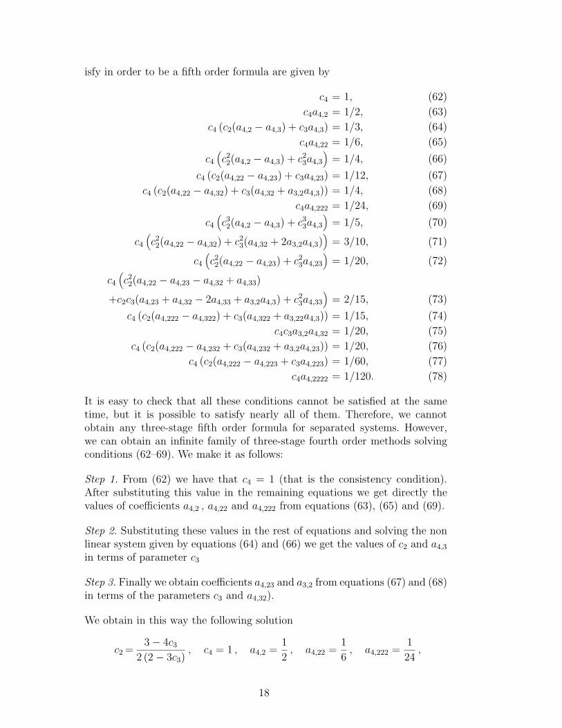
isfy in order to be a fifth order formula are given by

c4 = 1, (62)

c4a4,2 = 1/2, (63)

c4 (c2(a4,2 − a4,3) + c3a4,3) = 1/3, (64)

c4a4,22 = 1/6, (65)

c4

(c22(a4,2 − a4,3) + c2

3a4,3

)= 1/4, (66)

c4 (c2(a4,22 − a4,23) + c3a4,23) = 1/12, (67)

c4 (c2(a4,22 − a4,32) + c3(a4,32 + a3,2a4,3)) = 1/4, (68)

c4a4,222 = 1/24, (69)

c4

(c32(a4,2 − a4,3) + c3

3a4,3

)= 1/5, (70)

c4

(c22(a4,22 − a4,32) + c2

3(a4,32 + 2a3,2a4,3))

= 3/10, (71)

c4

(c22(a4,22 − a4,23) + c2

3a4,23

)= 1/20, (72)

c4

(c22(a4,22 − a4,23 − a4,32 + a4,33)

+c2c3(a4,23 + a4,32 − 2a4,33 + a3,2a4,3) + c23a4,33

)= 2/15, (73)

c4 (c2(a4,222 − a4,322) + c3(a4,322 + a3,22a4,3)) = 1/15, (74)

c4c3a3,2a4,32 = 1/20, (75)

c4 (c2(a4,222 − a4,232 + c3(a4,232 + a3,2a4,23)) = 1/20, (76)

c4 (c2(a4,222 − a4,223 + c3a4,223) = 1/60, (77)

c4a4,2222 = 1/120. (78)

It is easy to check that all these conditions cannot be satisfied at the sametime, but it is possible to satisfy nearly all of them. Therefore, we cannotobtain any three-stage fifth order formula for separated systems. However,we can obtain an infinite family of three-stage fourth order methods solvingconditions (62–69). We make it as follows:

Step 1. From (62) we have that c4 = 1 (that is the consistency condition).After substituting this value in the remaining equations we get directly thevalues of coefficients a4,2 , a4,22 and a4,222 from equations (63), (65) and (69).

Step 2. Substituting these values in the rest of equations and solving the nonlinear system given by equations (64) and (66) we get the values of c2 and a4,3

in terms of parameter c3

Step 3. Finally we obtain coefficients a4,23 and a3,2 from equations (67) and (68)in terms of the parameters c3 and a4,32).

We obtain in this way the following solution

c2 =3− 4c3

2 (2− 3c3), c4 = 1 , a4,2 =

1

2, a4,22 =

1

6, a4,222 =

1

24,

18

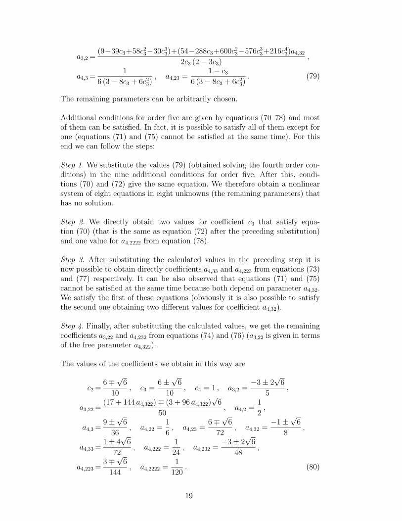
a3,2 =(9−39c3+58c2

3−30c33)+(54−288c3+600c2

3−576c33+216c4

3)a4,32

2c3 (2− 3c3),

a4,3 =1

6 (3− 8c3 + 6c23)

, a4,23 =1− c3

6 (3− 8c3 + 6c23)

. (79)

The remaining parameters can be arbitrarily chosen.

Additional conditions for order five are given by equations (70–78) and mostof them can be satisfied. In fact, it is possible to satisfy all of them except forone (equations (71) and (75) cannot be satisfied at the same time). For thisend we can follow the steps:

Step 1. We substitute the values (79) (obtained solving the fourth order con-ditions) in the nine additional conditions for order five. After this, condi-tions (70) and (72) give the same equation. We therefore obtain a nonlinearsystem of eight equations in eight unknowns (the remaining parameters) thathas no solution.

Step 2. We directly obtain two values for coefficient c3 that satisfy equa-tion (70) (that is the same as equation (72) after the preceding substitution)and one value for a4,2222 from equation (78).

Step 3. After substituting the calculated values in the preceding step it isnow possible to obtain directly coefficients a4,33 and a4,223 from equations (73)and (77) respectively. It can be also observed that equations (71) and (75)cannot be satisfied at the same time because both depend on parameter a4,32.We satisfy the first of these equations (obviously it is also possible to satisfythe second one obtaining two different values for coefficient a4,32).

Step 4. Finally, after substituting the calculated values, we get the remainingcoefficients a3,22 and a4,232 from equations (74) and (76) (a3,22 is given in termsof the free parameter a4,322).

The values of the coefficients we obtain in this way are

c2 =6∓√6

10, c3 =

6±√6

10, c4 = 1 , a3,2 =

−3± 2√

6

5,

a3,22 =(17 + 144 a4,322)∓ (3 + 96 a4,322)

√6

50, a4,2 =

1

2,

a4,3 =9±√6

36, a4,22 =

1

6, a4,23 =

6∓√6

72, a4,32 =

−1±√6

8,

a4,33 =1± 4

√6

72, a4,222 =

1

24, a4,232 =

−3± 2√

6

48,

a4,223 =3∓√6

144, a4,2222 =

1

120. (80)

19

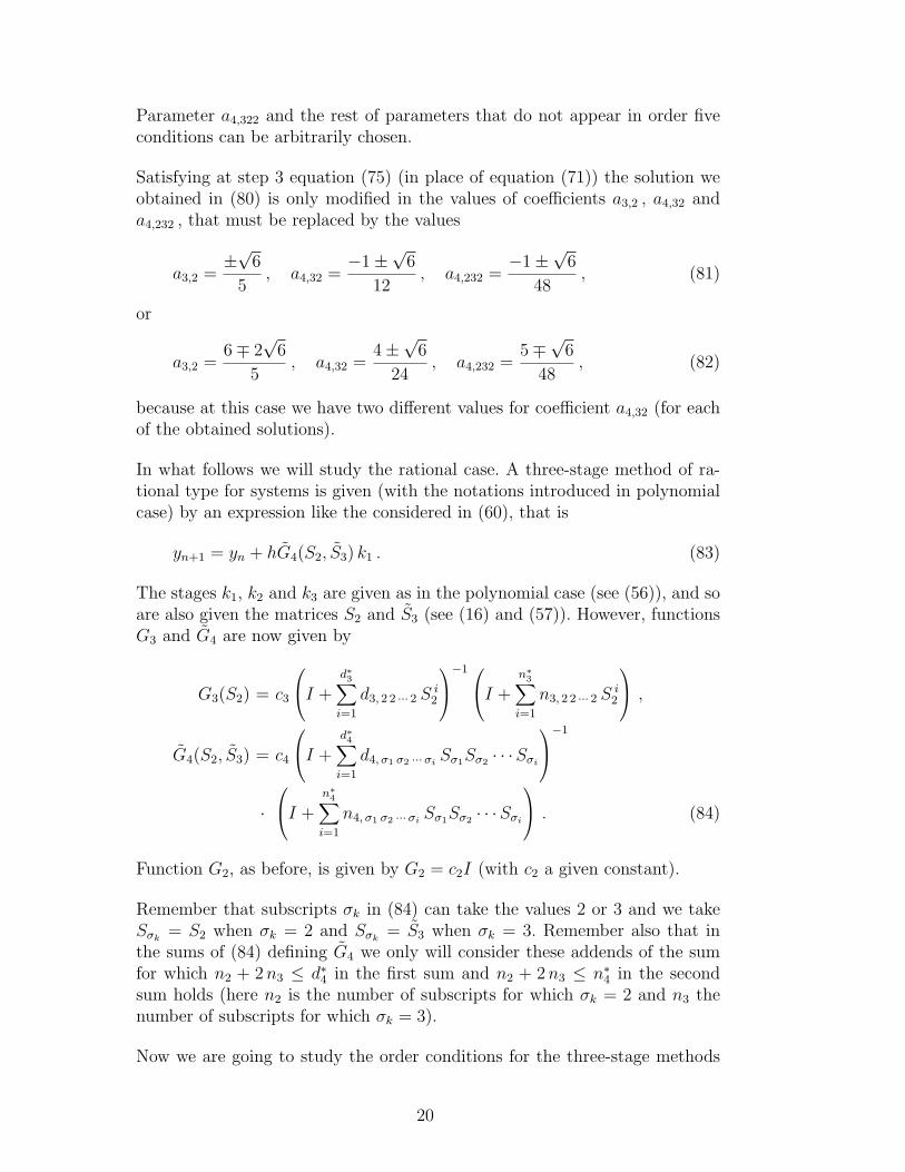
Parameter a4,322 and the rest of parameters that do not appear in order fiveconditions can be arbitrarily chosen.

Satisfying at step 3 equation (75) (in place of equation (71)) the solution weobtained in (80) is only modified in the values of coefficients a3,2 , a4,32 anda4,232 , that must be replaced by the values

a3,2 =±√6

5, a4,32 =

−1±√6

12, a4,232 =

−1±√6

48, (81)

or

a3,2 =6∓ 2

√6

5, a4,32 =

4±√6

24, a4,232 =

5∓√6

48, (82)

because at this case we have two different values for coefficient a4,32 (for eachof the obtained solutions).

In what follows we will study the rational case. A three-stage method of ra-tional type for systems is given (with the notations introduced in polynomialcase) by an expression like the considered in (60), that is

yn+1 = yn + hG4(S2, S3) k1 . (83)

The stages k1, k2 and k3 are given as in the polynomial case (see (56)), and soare also given the matrices S2 and S3 (see (16) and (57)). However, functionsG3 and G4 are now given by

G3(S2) = c3

I +

d∗3∑

i=1

d3, 2 2 ··· 2 S i2

−1

I +n∗3∑

i=1

n3, 2 2 ··· 2 S i2

,

G4(S2, S3) = c4

I +

d∗4∑

i=1

d4, σ1 σ2 ···σiSσ1Sσ2 · · ·Sσi

−1

·I +

n∗4∑

i=1

n4, σ1 σ2 ···σiSσ1Sσ2 · · ·Sσi

. (84)

Function G2, as before, is given by G2 = c2I (with c2 a given constant).

Remember that subscripts σk in (84) can take the values 2 or 3 and we takeSσk

= S2 when σk = 2 and Sσk= S3 when σk = 3. Remember also that in

the sums of (84) defining G4 we only will consider these addends of the sumfor which n2 + 2 n3 ≤ d∗4 in the first sum and n2 + 2 n3 ≤ n∗4 in the secondsum holds (here n2 is the number of subscripts for which σk = 2 and n3 thenumber of subscripts for which σk = 3).

Now we are going to study the order conditions for the three-stage methods

20

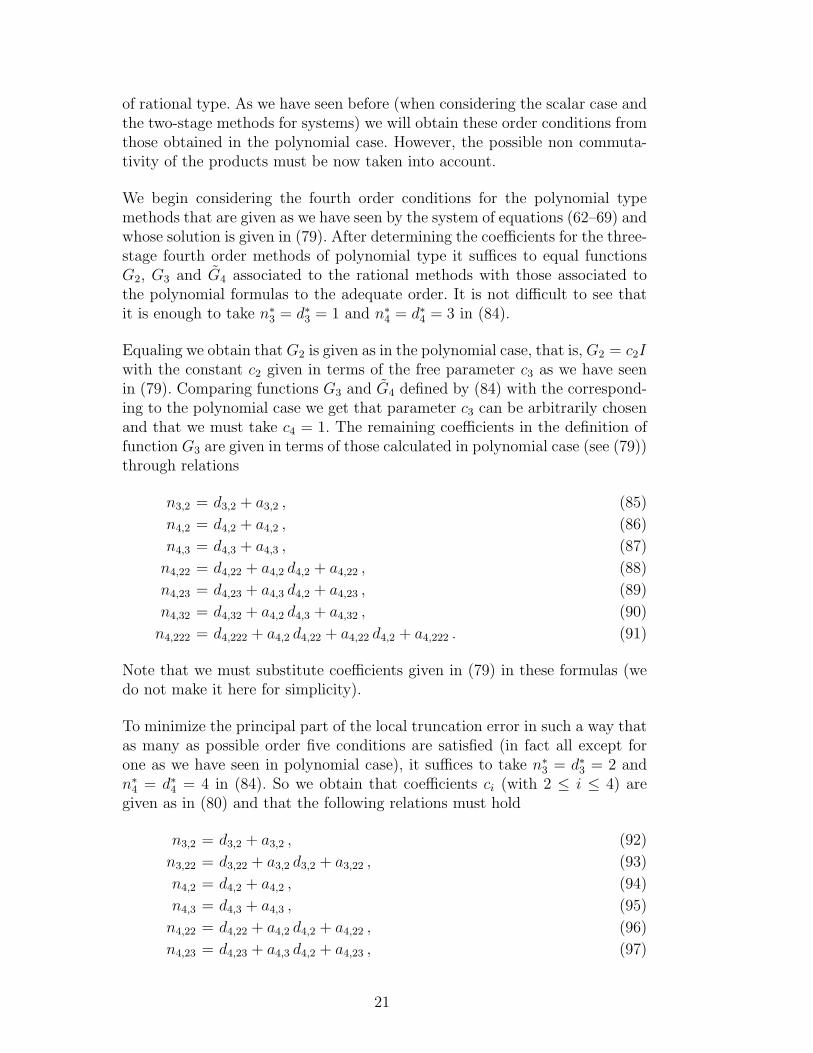
of rational type. As we have seen before (when considering the scalar case andthe two-stage methods for systems) we will obtain these order conditions fromthose obtained in the polynomial case. However, the possible non commuta-tivity of the products must be now taken into account.

We begin considering the fourth order conditions for the polynomial typemethods that are given as we have seen by the system of equations (62–69) andwhose solution is given in (79). After determining the coefficients for the three-stage fourth order methods of polynomial type it suffices to equal functionsG2, G3 and G4 associated to the rational methods with those associated tothe polynomial formulas to the adequate order. It is not difficult to see thatit is enough to take n∗3 = d∗3 = 1 and n∗4 = d∗4 = 3 in (84).

Equaling we obtain that G2 is given as in the polynomial case, that is, G2 = c2Iwith the constant c2 given in terms of the free parameter c3 as we have seenin (79). Comparing functions G3 and G4 defined by (84) with the correspond-ing to the polynomial case we get that parameter c3 can be arbitrarily chosenand that we must take c4 = 1. The remaining coefficients in the definition offunction G3 are given in terms of those calculated in polynomial case (see (79))through relations

n3,2 = d3,2 + a3,2 , (85)

n4,2 = d4,2 + a4,2 , (86)

n4,3 = d4,3 + a4,3 , (87)

n4,22 = d4,22 + a4,2 d4,2 + a4,22 , (88)

n4,23 = d4,23 + a4,3 d4,2 + a4,23 , (89)

n4,32 = d4,32 + a4,2 d4,3 + a4,32 , (90)

n4,222 = d4,222 + a4,2 d4,22 + a4,22 d4,2 + a4,222 . (91)

Note that we must substitute coefficients given in (79) in these formulas (wedo not make it here for simplicity).

To minimize the principal part of the local truncation error in such a way thatas many as possible order five conditions are satisfied (in fact all except forone as we have seen in polynomial case), it suffices to take n∗3 = d∗3 = 2 andn∗4 = d∗4 = 4 in (84). So we obtain that coefficients ci (with 2 ≤ i ≤ 4) aregiven as in (80) and that the following relations must hold

n3,2 = d3,2 + a3,2 , (92)

n3,22 = d3,22 + a3,2 d3,2 + a3,22 , (93)

n4,2 = d4,2 + a4,2 , (94)

n4,3 = d4,3 + a4,3 , (95)

n4,22 = d4,22 + a4,2 d4,2 + a4,22 , (96)

n4,23 = d4,23 + a4,3 d4,2 + a4,23 , (97)

21

n4,32 = d4,32 + a4,2 d4,3 + a4,32 , (98)

n4,33 = d4,33 + a4,3 d4,3 + a4,33 , (99)

n4,222 = d4,222 + a4,2 d4,22 + a4,22 d4,2 + a4,222 , (100)

n4,223 = d4,223 + a4,3 d4,22 + a4,23 d4,2 + a4,223 , (101)

n4,232 = d4,232 + a4,2 d4,23 + a4,32 d4,2 + a4,232 , (102)

n4,322 = d4,322 + a4,2 d4,32 + a4,22 d4,3 + a4,322 , (103)

n4,2222 = d4,2222 + a4,2 d4,222 + a4,22 d4,22 + a4,222 d4,2 + a4,2222 . (104)

In the preceding relations we must substitute coefficients (80) (modified andcompleted if desired with (81) and (82)).

9 Linear stability function of the methods for systems.

The study of the linear stability properties of the methods for systems is nowmore complicated that in scalar autonomous case. This is so because whenstudying formulas for separated systems we must consider in place of the testequation y′ = λ y with λ ∈ C, the system test y′ = Ay where A is a squarematrix of dimension m with m different eigenvalues λi ∈ C (1 ≤ i ≤ m) withnegative real parts. With the preceding conditions we know that the exactsolution to this system tends to zero when x tends to infinity and that thereexists a non singular matrix Q with Q−1AQ = Λ = diag[λ1, λ2, . . . , λm]. Thetransformation y = Qz enables us to simplify the study of the linear stabilityproperties of our methods. In fact, this study is reduced to consider the scalartest equation because the system test and the difference formulas defining ourmethods are uncoupled with the preceding transformation. In order to see thatthis is so it suffices to apply any p-stage method for systems (given by (5–7))to the system test y′ = Ay (satisfying all the above mentioned conditions)obtaining in this way

yn+1 = yn + hGp+1(S2, S3, . . . , Sp) k1 , (105)

where now the stages ki are given recursively by

k1 = Ayn

k2 = A (I + hG2 A) yn

k3 = A (I + hG3(hA) A) yn (106)...

kp = A (I + hGp(hA, hA, . . . , hA) A) yn ,

because, applied to the system, the square matrices Si satisfy Si = h A (fori = 2, 3, . . . , p).

22

We now define yn = Qwn and ki = Qαi (for i = 1, 2, . . . , p), that is we applythe transformation to uncouple the system. After multiplying by Q−1 rela-tions (105) and (106) and making the preceding transformation (rememberingthat Q−1AQ = Λ) we get

wn+1 = wn + hGp+1(hΛ, hΛ, . . . , hΛ)) α1 , (107)

with the stages given recursively by

α1 = Λ wn

α2 = Λ (I + hG2 Λ) wn

α3 = Λ (I + hG3(hΛ) Λ) wn (108)...

αp = Λ (I + hGp(hΛ, hΛ, . . . , hΛ) Λ) wn ,

as can be easily seen observing that relation Q−1Gi(hA, hA, . . . , hA) AQ =Gi(hΛ, hΛ, . . . , hΛ) Λ holds.

We have seen in this way that the difference systems defining our methods(when applied to the test system) are uncoupled with the transformation y =Qw , and obviously the system test is also uncoupled to the form w′ = Λ wby this transformation. For this reason, in what follows it suffices to considerthe scalar test equation given by y′ = λy with λ ∈ C and <(λ) < 0, whenstudying the linear stability properties of the methods for separated systems.

When we apply a p-stage method for systems defined by (5–7) to the scalartest equation, we obtain

yn+1 = R(z) yn , (109)

where R(z) is the linear stability function associated, with z = hλ. From (5–7)we obtain recursively

k1 = λ yn

S2 = z

S3 = z (110)...

Sp = z ,

and therefore the linear stability function takes the form

R(z) = 1 + z Gp+1(z, z, . . . , z) . (111)

Note that with the modification in the definition of matrices Si (by includingfunctions Gi) with respect to scalar case, the linear stability function is now

23

given in a more simple form than in the similar expression given in [7].

At this point we also note that with the modification introduced when studyingthe three-stage methods for separated systems by introducing the matrix termS3 = S3 − S2, we have from (110) that S3 = 0 (when method is applied toscalar test equation). Therefore the linear stability function is given in thiscase by R(z) = 1 + z G4(z, 0) , as can be deduced from (60).

10 A first example of L-stable three-stage method of order four.

We have seen before an example of L-stable two-stage method of order threefor separated systems, together with some numerical experiments to illustratethe good performance of this formula when applied to different stiff problems.

We also obtained the general form for the three-stage methods of order fourfor separated systems. Obviously most of these methods are not interestingbecause of the high computational cost associated. However, many of themethods perform well in many problems because of the high order obtainedan the good linear stability properties (the formulas contain approximationsto the Jacobian matrix with no additional function evaluations). To reduce thecomputational cost associated we will only consider those formulas for whichonly one LU factorization per step is necessary. We also will look for methodswith good linear stability properties such as A-stability and L-stability, inorder to obtain formulas that perform well when applied to stiff problems.

In what follows we are going to see a first example of a three-stage L-stablemethod of order four for separated systems. We look for methods whose as-sociated linear stability function is a rational function with only one real pole(so that only one LU factorization per integration step is necessary) as oc-curs, for example, with the SDIRK methods. It is not difficult to see that toobtain an order four L-stable method, whose linear stability function has anunique real pole, the multiplicity of this pole must be greater or equal thanfour. There exists only one real value of the pole that enable us to obtain thepreceding properties with multiplicity four, and this value is given by the rootof polynomial

24 x4 − 96 x3 + 72 x2 − 16 x + 1 , (112)

that takes approximately the value a ≈ 0.57281606 (see [11], pp. 96–98 formore details). The corresponding linear stability function is the rational func-tion R(z) with numerator of degree three and denominator of degree four, that

24

is given in terms of the preceding value a by

R(z) =6+6(1−4a)z+3(1−8a+12a2)z2+(1−12a+36a2−24a3)z3

6 (1− a z)4. (113)

We can obtain a method satisfying all the above requirements as follows:

Step 1. We take the following values for the free parameters a4,32 and c3 in (79)

a4,32 = 0 , c3 =6 +

√6

10. (114)

Note that the value we are taking for c3 is the same we obtained for three-stagefifth order methods in scalar case.

Step 2. We substitute these values in (79) and the so obtained solution (thatassures order four for the three-stage methods of polynomial type) in rela-tions (85–91). We obtain in this way a family of three-stage fourth ordermethods of rational type. Note that any of these formulas is completely de-termined from the values of the coefficients d∗.

Step 3. Finally, between all these many options that we have in order to obtaina method with the desired linear stability function, we take this obtained bymaking zero the following coefficients

d4,3 = d4,23 = d4,32 = 0 , (115)

and taking

d3,2 = −a , (116)

we obtain in terms of the above mentioned value a the solution

c2 =6−√6

10, c3 =

6 +√

6

10, c4 = 1 , d3,2 = −a ,

d4,2 =−4 a , d4,3 = 0 , d4,22 = 6 a2 , d4,23 = 0 , d4,32 = 0 ,

d4,222 =−4 a3 , d4,2222 = a4 , n3,2 =(6− 5 a)−√6

5,

n4,2 =1− 8 a

2, n4,3 =

9 +√

6

36, n4,22 =

36 a2 − 12 a + 1

6,

n4,23 =6 (1− 12 a)− (1 + 8 a)

√6

72, n4,32 = 0 ,

n4,222 =−96 a3 + 72 a2 − 16 a + 1

24. (117)

The remaining parameters are taken equal to zero.

25

Note that in the preceding formula we have introduced the coefficient d4,2222

that do not appear in fourth order conditions. We make it because, as we havecommented before, to obtain L-stability the denominator in the associatedlinear stability function (113) must be of degree four.

Now we will briefly comment why we make zero the coefficients in (115). Wemake zero the coefficients d∗ in (115) corresponding to those terms with atleast one the factor S3, that is, the coefficient has at least one 3 in the subscript.We make this so that when making the LU factorization only the matrix S2

appears.

We have taken the parameter d3,2 = −a in (116) so that no additional LUfactorizations are necessary to calculate the stages (in fact stage k3). It seemsbetter to reduce the computational cost associated with the method by makingzero coefficient d3,2 in (116), but different numerical experiments show thatwith this choice for the parameter the errors grow when integrating many stiffproblems with moderate stepsizes h.

Note at this point that the three-stage fourth order L-stable formula we haveobtained (and other formulas we can obtain in a similar way) performs better,with respect to number of function evaluations per integration step, thanSDIRK methods of Runge-Kutta type. In [11], pp. 98 it is shown that atleast four stages are necessary to obtain a SDIRK formula of order four andL-stable.

In what follows, we will illustrate with some numerical experiments the per-formance of the obtained L-stable formula.

11 Some numerical experiments with stiff problems.

We now repeat the numerical experiments of the preceding sections with ournew three-stage fourth order L-stable method.

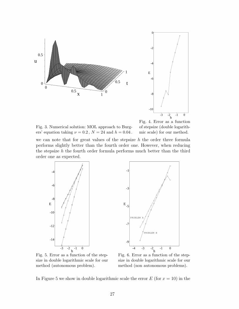
When we apply this method to the ODE system associated to Burgers’ equa-tion (by the MOL approach) that we described in (23), taking the valuesN = 24 and ν = 0.2 and integrating with fixed stepsize h = 0.04 , we obtainthe Figure 3 for the numerical solution. This figure is very similar to Figure 1obtained in [6] for the two-stage third order method.

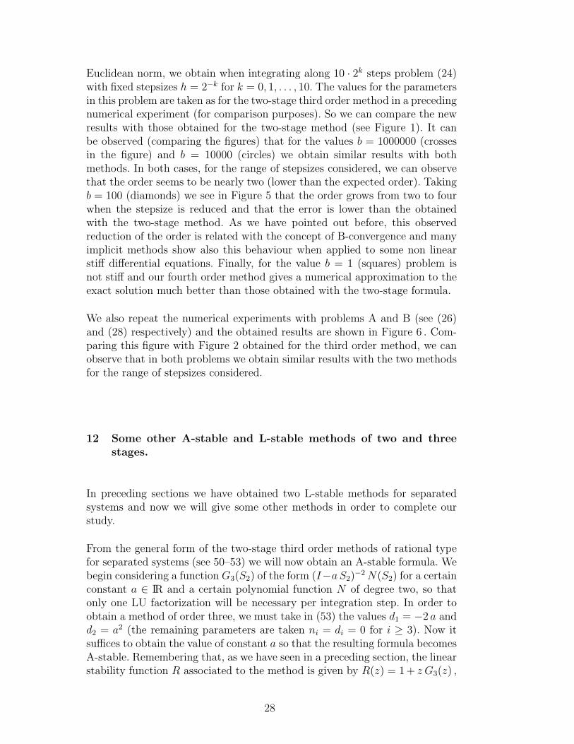
In Figure 4 we show, in double logarithmic scale, the error E (in the Euclideannorm in IR24) at point t = 1 that we obtain integrating with fixed stepsizeh = 2−k for k = 2, 3, . . . , 10 the preceding problem. When comparing thisfigure with the Figure 2 obtained in [6] for the two-stage third order method,

26

00.5

1 x 0

0.5

1

t0

0.5

u

Fig. 3. Numerical solution: MOL approach to Burg-ers’ equation taking ν = 0.2 , N = 24 and h = 0.04 .

-10

-8

-6

-4

-2

0

E

-3 -2 -1 0h

Fig. 4. Error as a functionof stepsize (double logarith-mic scale) for our method.

we can note that for great values of the stepsize h the order three formulaperforms slightly better than the fourth order one. However, when reducingthe stepsize h the fourth order formula performs much better than the thirdorder one as expected.

-14

-12

-10

-8

-6

-4

E

-3 -2 -1 0h

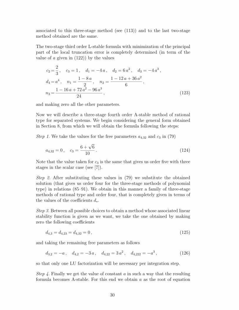
Fig. 5. Error as a function of the step-size in double logarithmic scale for ourmethod (autonomous problem).

PROBLEM A

PROBLEM B

-9

-7

-5

-3

-1

E

-4 -3 -2 -1 0h

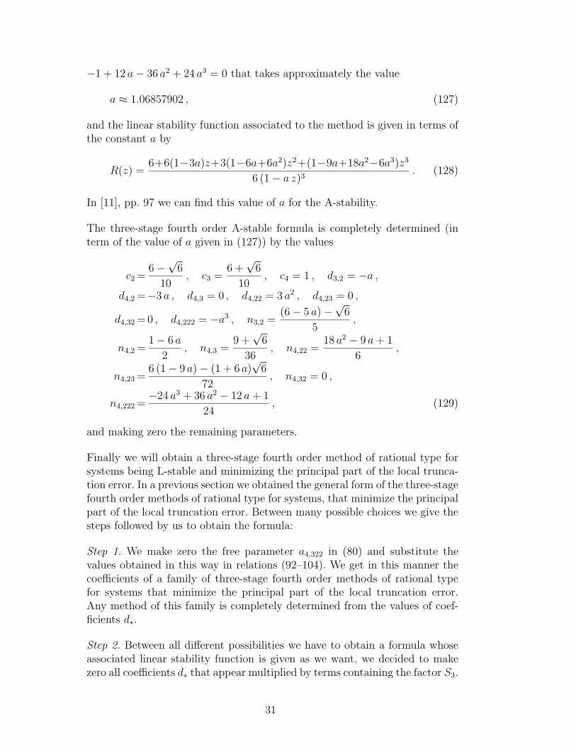
Fig. 6. Error as a function of the step-size in double logarithmic scale for ourmethod (non autonomous problems).

In Figure 5 we show in double logarithmic scale the error E (for x = 10) in the

27

Euclidean norm, we obtain when integrating along 10 · 2k steps problem (24)with fixed stepsizes h = 2−k for k = 0, 1, . . . , 10. The values for the parametersin this problem are taken as for the two-stage third order method in a precedingnumerical experiment (for comparison purposes). So we can compare the newresults with those obtained for the two-stage method (see Figure 1). It canbe observed (comparing the figures) that for the values b = 1000000 (crossesin the figure) and b = 10000 (circles) we obtain similar results with bothmethods. In both cases, for the range of stepsizes considered, we can observethat the order seems to be nearly two (lower than the expected order). Takingb = 100 (diamonds) we see in Figure 5 that the order grows from two to fourwhen the stepsize is reduced and that the error is lower than the obtainedwith the two-stage method. As we have pointed out before, this observedreduction of the order is related with the concept of B-convergence and manyimplicit methods show also this behaviour when applied to some non linearstiff differential equations. Finally, for the value b = 1 (squares) problem isnot stiff and our fourth order method gives a numerical approximation to theexact solution much better than those obtained with the two-stage formula.

We also repeat the numerical experiments with problems A and B (see (26)and (28) respectively) and the obtained results are shown in Figure 6 . Com-paring this figure with Figure 2 obtained for the third order method, we canobserve that in both problems we obtain similar results with the two methodsfor the range of stepsizes considered.

12 Some other A-stable and L-stable methods of two and threestages.

In preceding sections we have obtained two L-stable methods for separatedsystems and now we will give some other methods in order to complete ourstudy.

From the general form of the two-stage third order methods of rational typefor separated systems (see 50–53) we will now obtain an A-stable formula. Webegin considering a function G3(S2) of the form (I−a S2)

−2 N(S2) for a certainconstant a ∈ IR and a certain polynomial function N of degree two, so thatonly one LU factorization will be necessary per integration step. In order toobtain a method of order three, we must take in (53) the values d1 = −2 a andd2 = a2 (the remaining parameters are taken ni = di = 0 for i ≥ 3). Now itsuffices to obtain the value of constant a so that the resulting formula becomesA-stable. Remembering that, as we have seen in a preceding section, the linearstability function R associated to the method is given by R(z) = 1 + z G3(z) ,

28

we obtain

R(z) =6 + 6 (1− 2a) z + 3 (1− 4a + 2a2) z2 + (1− 6a + 6a2) z3

6 (1− a z)2, (118)

and we get the value of constant a making zero the coefficient of z3 in thenumerator of (118), that is, solving equation 1− 6a + 6a2 = 0. From the twodifferent values we obtain in this way we have that the one for A-stability isgiven by

a =3 +

√3

6≈ 0.78867513 . (119)

For more details related to the A-stability associated to the above functionR(z), the book [11] pp. 97 is again a good reference. Summarizing, the valuesof the parameters we must take in order to obtain the A-stable two-stage thirdorder method for separated systems are given by

c2 =2

3, c3 = 1, d1 = −3+

√3

3, d2 =

2+√

3

6, n1 = −3+2

√3

6. (120)

We now are going to see how to obtain a L-stable two-stage third order methodof rational type for systems that minimizes the principal part of the localtruncation error. To this end we begin considering the general form (50–52),but where now function G3 takes the form (54), from which we can concludethat the method satisfies all the required properties except for the L-stability.As for other methods obtained previously, we take function G3(S2) of theform (I−aS2)

−4 N(S2) for a certain constant a ∈ IR and a certain polynomialfunction N of degree three. This moves us to take in (54) the values d1 = −4 a,d2 = 6 a2, d3 = −4 a3 and d4 = a4 (the remaining parameters di take the valuezero and ni = 0 for i ≥ 4). The value of the constant a is determined in sucha way that the resulting formula is L-stable. Making zero the coefficient of z4

in the numerator of the linear stability function R(z), it is easy to check thatwe obtain the following linear stability function

R(z) =6+6(1−4a)z+3(1−8a+12a2)z2+(1−12a+36a2−24a3)z3

6 (1− a z)4, (121)

for the resulting L-stable method, in terms of the value of a that is given as theroot of polynomial 1−16 a+72 a2−96 a3 +24 a4 = 0 that takes approximatelythe value

a ≈ 0.57281606 . (122)

In [11], pp. 98 we can find this value of a for the L-stability. Note that thevalue of a in (122) is the same that we obtained in Section 10 for the three-stage fourth order L-stable formula. Moreover, the linear stability function

29

associated to this three-stage method (see (113)) and to the last two-stagemethod obtained are the same.

The two-stage third order L-stable formula with minimization of the principalpart of the local truncation error is completely determined (in term of thevalue of a given in (122)) by the values

c2 =2

3, c3 = 1 , d1 = −4 a , d2 = 6 a2 , d3 = −4 a3 ,

d4 = a4 , n1 =1− 8 a

2, n2 =

1− 12 a + 36 a2

6,

n3 =1− 16 a + 72 a2 − 96 a3

24, (123)

and making zero all the other parameters.

Now we will describe a three-stage fourth order A-stable method of rationaltype for separated systems. We begin considering the general form obtainedin Section 8, from which we will obtain the formula following the steps:

Step 1. We take the values for the free parameters a4,32 and c3 in (79)

a4,32 = 0 , c3 =6 +

√6

10. (124)

Note that the value taken for c3 is the same that gives us order five with threestages in the scalar case (see [7]).

Step 2. After substituting these values in (79) we substitute the obtainedsolution (that gives us order four for the three-stage methods of polynomialtype) in relations (85–91). We obtain in this manner a family of three-stagemethods of rational type and order four, that is completely given in terms ofthe values of the coefficients d∗.

Step 3. Between all possible choices to obtain a method whose associated linearstability function is given as we want, we take the one obtained by makingzero the following coefficients

d4,3 = d4,23 = d4,32 = 0 , (125)

and taking the remaining free parameters as follows

d3,2 = −a , d4,2 = −3 a , d4,22 = 3 a2 , d4,222 = −a3 , (126)

so that only one LU factorization will be necessary per integration step.

Step 4. Finally we get the value of constant a in such a way that the resultingformula becomes A-stable. For this end we obtain a as the root of equation

30

−1 + 12 a− 36 a2 + 24 a3 = 0 that takes approximately the value

a ≈ 1.06857902 , (127)

and the linear stability function associated to the method is given in terms ofthe constant a by

R(z) =6+6(1−3a)z+3(1−6a+6a2)z2+(1−9a+18a2−6a3)z3

6 (1− a z)3. (128)

In [11], pp. 97 we can find this value of a for the A-stability.

The three-stage fourth order A-stable formula is completely determined (interm of the value of a given in (127)) by the values

c2 =6−√6

10, c3 =

6 +√

6

10, c4 = 1 , d3,2 = −a ,

d4,2 =−3 a , d4,3 = 0 , d4,22 = 3 a2 , d4,23 = 0 ,

d4,32 = 0 , d4,222 = −a3 , n3,2 =(6− 5 a)−√6

5,

n4,2 =1− 6 a

2, n4,3 =

9 +√

6

36, n4,22 =

18 a2 − 9 a + 1

6,

n4,23 =6 (1− 9 a)− (1 + 6 a)

√6

72, n4,32 = 0 ,

n4,222 =−24 a3 + 36 a2 − 12 a + 1

24, (129)

and making zero the remaining parameters.

Finally we will obtain a three-stage fourth order method of rational type forsystems being L-stable and minimizing the principal part of the local trunca-tion error. In a previous section we obtained the general form of the three-stagefourth order methods of rational type for systems, that minimize the principalpart of the local truncation error. Between many possible choices we give thesteps followed by us to obtain the formula:

Step 1. We make zero the free parameter a4,322 in (80) and substitute thevalues obtained in this way in relations (92–104). We get in this manner thecoefficients of a family of three-stage fourth order methods of rational typefor systems that minimize the principal part of the local truncation error.Any method of this family is completely determined from the values of coef-ficients d∗.

Step 2. Between all different possibilities we have to obtain a formula whoseassociated linear stability function is given as we want, we decided to makezero all coefficients d∗ that appear multiplied by terms containing the factor S3.

31

The remaining free parameters are taken as follows

d3,2 =−2 a , d3,22 = a2 , d4,2 = −5 a , d4,22 = 10 a2 ,

d4,222 =−10 a3 , d4,2222 = 5 a4 , d4,22222 = −a5 . (130)

In the preceding formula we have introduced coefficient d4,22222 which does notappear neither in order four conditions nor in order five conditions (that wetake into account to minimize the principal part of the local truncation error).We make this because we look for a L-stable method and so the linear stabilityfunction associated to the formula must have a denominator of degree five.

Step 3. Finally we get the value of constant a in such a way that the resultingformula is L-stable. We must take a as the root of polynomial −1 + 25 a −200 a2 + 600 a3 − 600 a4 + 120 a5 = 0 that takes approximately the value

a ≈ 0.27805384 , (131)

and the linear stability function R(z) associated to the resulting method isgiven in terms of a by

R(z) =24+24(1−5a)z+12(1−10a+20a2)z2

24 (1− a z)5(132)

+4(1−15a+60a2−60a3)z3+(1−20a+120a2−240a3+120a4)z4

24 (1− a z)5.

In [11], pp. 98 we can find this value of a giving us the L-stability property.

The obtained coefficients for the method are given by

c2 =6−√6

10, c3 =

6 +√

6

10, c4 = 1 , d3,2 = −2 a ,

d3,22 = a2 , d4,2 = −5 a , d4,22 = 10 a2 , d4,222 = −10 a3 ,

d4,2222 = 5 a4 , d4,22222 = −a5 , n3,2 =−(3 + 10 a) + 2

√6

5,

n3,22 =(17 + 60 a + 50 a2)− (3 + 40 a)

√6

50, n4,2 =

1− 10 a

2,

n4,3 =9 +

√6

36, n4,22 =

60 a2 − 15 a + 1

6,

n4,23 =6 (1− 15 a)− (1 + 10 a)

√6

72, n4,32 =

−1 +√

6

8,

n4,33 =1 + 4

√6

72, n4,222 =

−240 a3 + 120 a2 − 20 a + 1

24,

n4,223 =3 (1− 20 a + 120 a2) + (−1 + 10 a + 40 a2)

√6

144,

32

n4,232 =3 (−1 + 10 a) + 2(1− 15 a)

√6

48,

n4,2222 =600 a4 − 600 a3 + 200 a2 − 25 a + 1

120, (133)

in terms of the value of a given in (131) and making zero the remaining freeparameters.

13 Numerical experiments with the two and three-stage A-stableand L-stable methods: Van der Pol’s equation.

In order to illustrate the good behaviour of the GRK-methods obtained wewill now study some numerical experiments. We will apply our methods tosome problems and compare the results obtained with those we get with someclassical formulas.

The first problem we consider, involves the well known Van der Pol’s equationthat is given by

ε z′′ + (z2 − 1) z′ + z = 0 , z(0) = a , z′(0) = b . (134)

Note that our methods cannot be applied to the system of first order ODEsgiven by

z′ = y z(0) = a

y′ =1

ε((1− z2) y − z) y(0) = b

(135)

we obtain transforming in the usual way this second order equation, becausethe resulting system is not a separates one. However, using Lienard’s coordi-nates (see [11], pp. 372 for more details) the problem (134) takes the form

y′ = −z y(0) = ε b− a +a3

3

z′ =1

ε

(y + z − z3

3

)z(0) = a

(136)

and now our methods can be applied to this system.

We integrate this problem in the interval [0, 0.5] , taking ε = 10−5. We haveconsidered the following initial conditions

y(0) = 0.66666000001234554549467 , z(0) = 2. , (137)

obtained from those considered in [11], pp. 403, by taking the Lienard’s co-

33

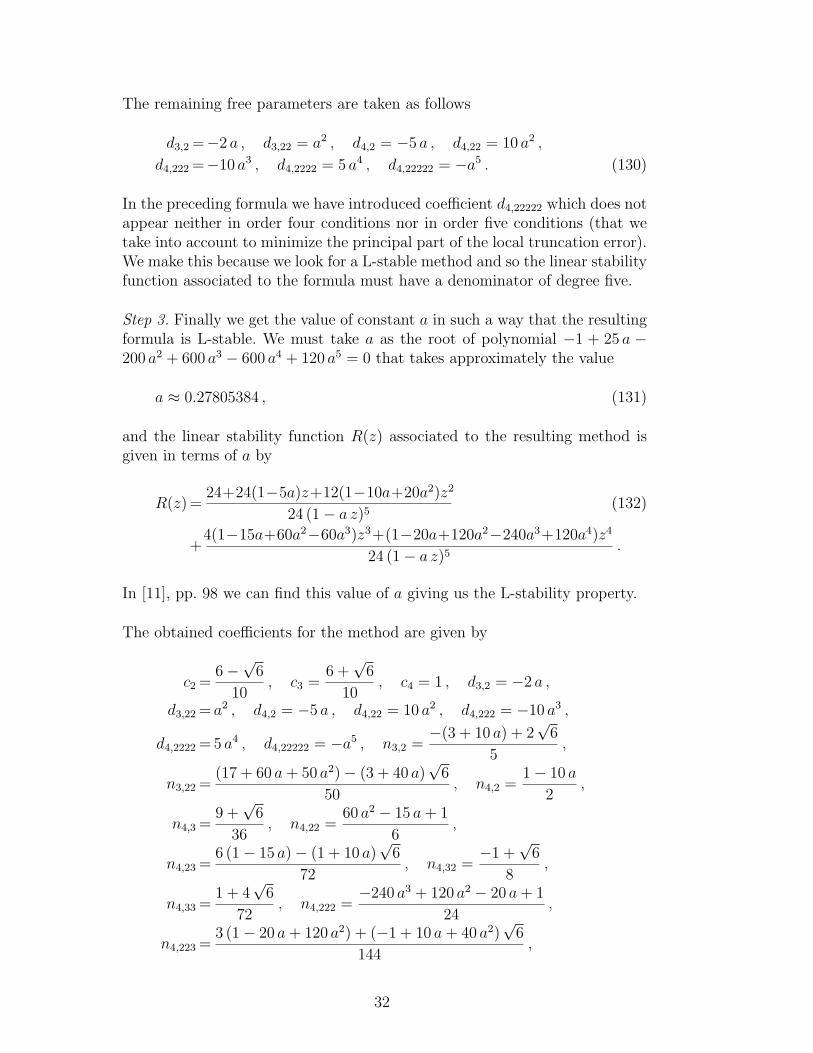
ordinates. With the six methods obtained, we have integrated the precedingproblem with fixed stepsize h and we have calculated the relative error ob-tained in both components at the point 0.5. Errors are measured with respectto a reference solution obtained with a very accurate variable step method (the’gear’ method implemented in MAPLEV, working with 30 digits and takinga tolerance of 10−20) that is enough for our purposes.

For comparison purposes we have also integrated this problem with the two-stage third order Rosenbrock method that can be found for example in [10],pp. 334, and known as Calahan’s method.

-16

-13

-10

-7

-4

-1

E

-5 -4 -3 -2 -1h

Fig. 7. Relative error (first component)as a function of the stepsize in dou-ble logarithmic scale for the third ordermethods.

-11

-9

-7

-5

-3

-1

E

-5 -4 -3 -2 -1h

Fig. 8. Relative error (second compo-nent) as a function of the stepsize indouble logarithmic scale for the thirdorder methods.

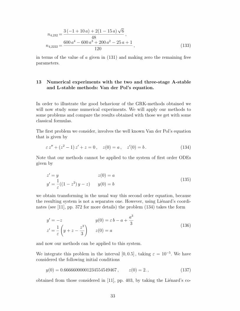
In Figures 7 and 8 we show the relative errors corresponding to the first andsecond components respectively as a function of the stepsize h (taking h =0.1 ·2−k for k = 0, 1, 2, . . . , 12) in double logarithmic scale for the different thirdorder methods. Calahan’s method is represented in these figures by squares.With diamonds we represent the third order A-stable method, with circles thefirst third order L-stable formula we obtained and with crosses the last thirdorder L-stable method we have developed.

It can be observed in these figures that Calahan’s method performs better thanour three methods when big values of the stepsize are considered. When wetake smaller stepsizes our methods perform very similarly to Calahan’s formulaand some of them perform even better than this Rosenbrock formula. Noteat this point that the problem considered is very stiff, with one of the eigen-values of the associated Jacobian matrix in the interval [−300000,−150000]

34

and the other eigenvalue being small and negative along the integration in-terval. Note also that Calahan’s method needs an evaluation of the Jacobianmatrix associated to the problem per integration step and that our methods,as we have pointed out before, incorporate an approximation to this Jacobianmatrix obtained from matrix S2/h (with no extra evaluations). This explainswhat happens when the stepsize h is big, because when this is so we havethat the approximation that gives matrix S2 to the Jacobian matrix is usuallynot too good (and in some problems this gives worse approximations to thesolution). It can be expected that this formulas will perform better by usingvariable stepsizes, but we will not study this here.

-16

-13

-10

-7

-4

-1

E

-5 -4 -3 -2 -1h

Fig. 9. Relative error (first component)as a function of the stepsize in doublelogarithmic scale for the fourth ordermethods.

-11

-9

-7

-5

-3

-1

E

-5 -4 -3 -2 -1h

Fig. 10. Relative error (second compo-nent) as a function of the stepsize indouble logarithmic scale for the fourthorder methods.

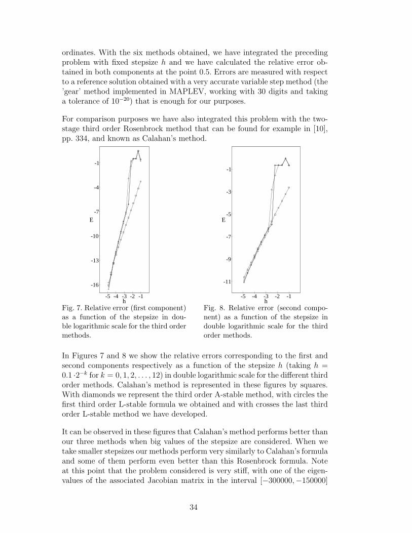
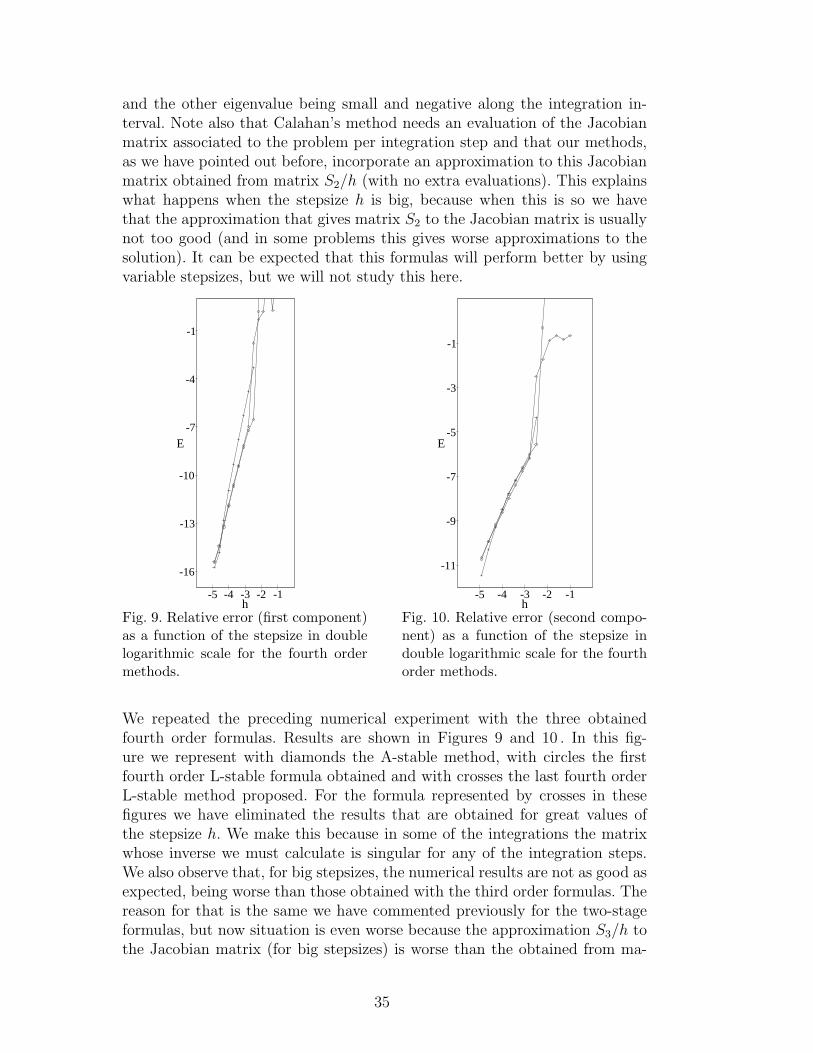
We repeated the preceding numerical experiment with the three obtainedfourth order formulas. Results are shown in Figures 9 and 10 . In this fig-ure we represent with diamonds the A-stable method, with circles the firstfourth order L-stable formula obtained and with crosses the last fourth orderL-stable method proposed. For the formula represented by crosses in thesefigures we have eliminated the results that are obtained for great values ofthe stepsize h. We make this because in some of the integrations the matrixwhose inverse we must calculate is singular for any of the integration steps.We also observe that, for big stepsizes, the numerical results are not as good asexpected, being worse than those obtained with the third order formulas. Thereason for that is the same we have commented previously for the two-stageformulas, but now situation is even worse because the approximation S3/h tothe Jacobian matrix (for big stepsizes) is worse than the obtained from ma-

35

trix S2/h. However, it can be observed that reducing the stepsize situation israpidly much better.

Even though the two and three-stage formulas proposed have some problemsfor moderate stepsizes (as we have pointed out before) they give good ap-proximations to the exact solution of the problem. In fact, we obtain goodapproximations to the solution integrating with stepsizes much greater thanthose we can consider when integrating with any classical explicit formula.The order reduction observed for this problem also occurs for other A-stableand L-stable Runge-Kutta type formulas (see [11], pp. 403–404).

14 Numerical experiments with the two and three-stage A-stableand L-stable methods: Burgers’ equation.

Now we will consider another problem. More precisely, we will repeat thenumerical experiment of a preceding section with the system of ODEs givenby (23). In this problem, obtained by the method of lines approach to theBurgers’ equation, we will consider the values N = 24 and ν = 0.2.

-8

-6

-4

-2

E

-3 -2 -1h

Fig. 11. Error as a function of the step-size in double logarithmic scale for thethird order methods.

-10

-8

-6

-4

-2

E

-3 -2 -1h

Fig. 12. Error as a function of the step-size in double logarithmic scale for thefourth order methods.

In Figure 11 we show in double logarithmic scale the error E (measured withthe Euclidean norm in IR24) at the point t = 1, obtained by integrating thisproblem with the different third order methods, taking fixed stepsize h = 2−k

for the values k = 3, 4, . . . , 10. We have represented the methods in this figure

36

with the same symbols as in Figures 7 and 8. It can be observed in the figurethat Calahan’s method performs slightly better than our proposed formulaswhen big values of the stepsize h are considered, but when this stepsize isreduced our methods perform very similarly to Calahan’s formula and someof them perform even better than the Calahan’s formula. For this problem thethree proposed formulas give very similar approximations to solution, as canbe seen in the figure. It is easily seen that the slopes of the curves representedin the figure are near to three (as expected).

When we repeat the last numerical experiment taking the three fourth ordermethods, we get Figure 12. We have represented the formulas in this figurewith the same symbols as in Figures 9 and 10. It can be observed that, for bigvalues of the stepsize, the approximations we get from the the fourth ordermethods are in some cases slightly worse than those obtained from the thirdorder methods. However, for smaller stepsizes the fourth order methods per-form much better than the third order ones. We also observe that the methodthat gives the better approximations for small stepsizes is that represented bycrosses in the figure (but this is also the method with the greatest computa-tional cost associated). The slopes of the curves represented in the figure arenearly four when the stepsize considered is reduced.

15 Conclusions.

In this second part we have introduced and studied a new family of methodsfor the numerical integration of some systems of ODEs. These new methodsseem quite promising, for instance in the context of solving some nonlinearparabolic equations (by the method of lines approach). We have shown thatwith the family of linearly implicit methods we have proposed here, it is possi-ble to attain order three with only two stages and order four with three stages,as well as some interesting linear stability properties such as A-stability andL-stability. Our methods do not require Jacobian evaluations in their imple-mentation and therefore require less computational work than other classicalimplicit and linearly implicit methods that can be applied to stiff problems.

In subsequent works we will study as in [2] how to obtain formulas (belongingto the family of GRK-methods) from any prefixed linear stability function.This can be of great interest when considering perturbed problems for whichthe exact solution of the unperturbed problem is known in advantage, be-cause we can obtain methods specifically designed to integrate exactly theunperturbed problem.

We will also extend our GRK-methods in order to obtain formulas with built-in error estimates, that is, embedded GRK-methods.

37

References

[1] R. Alexander, Diagonally implicit Runge-Kutta methods for stiff O.D.E.’s,SIAM J. Numer. Anal. 14 (1977) 1006–1021.

[2] J. Alvarez, Obtaining New Explicit Two-Stage Methods for the ScalarAutonomous IVP with Prefixed Stability Functions, Intl. Journal of AppliedSc. & Computations 6 (1999) 39–44.

[3] J. Alvarez, Metodos GRK para ecuaciones diferenciales ordinarias, Universidadde Valladolid, Spain, Dpto. de Matematica Aplicada a la Ingenierıa, Tesis -Ph.D. Thesis, 2002, 149 pp.

[4] J. Alvarez and J. Rojo, New A-stable explicit two-stage methods of order threefor the scalar autonomous IVP, in: P. de Oliveira, F. Oliveira, F. Patrıcio, J.A.Ferreira, A. Araujo, eds., Proc. of the 2nd. Meeting on Numerical Methods forDifferential Equations, NMDE’98 (Coimbra, Portugal, 1998) 57–66.

[5] J. Alvarez and J. Rojo, A New Family of Explicit Two-Stage Methods oforder Three for the Scalar Autonomous IVP, Intl. Journal of Applied Sc. &Computations 5 (1999) 246–251.

[6] J. Alvarez and J. Rojo, Special methods for the numerical integration of someODE’s systems, Nonlinear Analysis: Theory, Methods and Applications, 47(2001) 5703–5708.

[7] J. Alvarez and J. Rojo, An improved class of generalized Runge-Kuttamethods for stiff problems, Part I: The scalar case. Applied Mathematics andComputations 130 (2002) 537–560.

[8] J. Alvarez and J. Rojo, An improved class of generalized Runge-Kutta-Nystrom methods for special second order differential equations, in Proc. ofthe International Conference on Computational and Mathematical Methodsin Science and Engineering, CMMSE 2002 (Alicante, Spain, 2002) I 11–20.(Alicante, Spain).

[9] J.C. Butcher, Implicit Runge-Kutta processes, Math. Comp. 18 (1964) 50–64.

[10] J.C. Butcher, The Numerical Analysis of Ordinary Differential Equations:Runge-Kutta and General Linear Methods (Wiley, Chichester, 1987).

[11] E. Hairer and G. Wanner, Solving Ordinary Differential Equations II. Stiff andDifferential-Algebraic Problems (Springer-Verlag, Berlin, 1996).

[12] P. Kaps, Rosenbrock-type methods, in: G. Dahlquist and R. Jeltsch, eds.,Numerical methods for solving stiff initial value problems, Proceedings,Oberwolfach 28/6–4/7 1981, Bericht Nr. 9, Inst. fur Geometrie und PraktischeMathematik der RWTH Aachen (Aachen, Germany, 1981) 5 pp.

[13] P. Kaps, S. W. H. Poon and T. D. Bui, Rosenbrock Methods for StiffODEs: A Comparison of Richardson Extrapolation and Embedding Technique,Computing 34 (1985) 17–40.

38

[14] P. Kaps and P. Rentrop, Generalized Runge-Kutta Methods of Order Fourwith Stepsize Control for Stiff Ordinary Differential Equations, Numer. Math.33 (1979) 55–68.

[15] P. Kaps and G. Wanner, A Study of Rosenbrock-Type Methods of High Order,Numer. Math. 38 (1981) 279–298.

[16] J.D. Lambert, Numerical Methods for Ordinary Differential Systems. TheInitial Value Problem (Wiley, Chichester, 1991).

[17] S.P. Nørsett and A. Wolfbrandt, Order Conditions for Rosenbrock TypeMethods, Numer. Math. 32 (1979) 1–15.

[18] A. Prothero and A. Robinson, On the stability and accuracy of one-stepmethods for solving stiff systems of ordinary differential equations, Math.Comput. 28 (1974) 145–162.

[19] H.H. Rosenbrock, Some general implicit processes for the numerical solution ofdifferential equations, Comput. J. 5 (1963) 329–330.

[20] J.M. Sanz-Serna and M.P. Calvo, Numerical Hamiltonian Problems (Chapman-Hall, London, 1993).

[21] S. Scholz, Order Barriers for the B-Convergence of ROW Methods, Computing41 (1989) 219–235.

[22] T. Steihaug and A. Wolfbrandt, An Attempt to Avoid Exact Jacobian andNonlinear Equations in the Numerical Solution of Stiff Differential Equations,Math. Comp. 33 (1979) 521–534.

[23] J. G. Verwer, S-Stability Properties for Generalized Runge-Kutta Methods,Numer. Math. 27 (1977) 359–370.

[24] H. Zedan, Avoiding the exactness of the Jacobian matrix in Rosenbrockformulae, Comput. Math. Appl. 19 (1990) 83–89.

39