Applied Numerical Mathematics 34 (2000) 59–84

The choice of parameters in parallel general linear methods forstiff problems

J.C. Butcher∗, A.D. Singh1

Department of Mathematics, The University of Auckland, New Zealand

Abstract

The special type of general linear method known as a DIMSIM can be specialized to parallel computation forstiff initial value problems by considering type 4 methods. In this paper we consider an implementation of type 4methods withA = λI andp = s. We also consider some generalizations of the type 4 DIMSIMs in an effort tomake these methods more efficient. 2000 IMACS. Published by Elsevier Science B.V. All rights reserved.

Keywords:Linear methods; Stiff problems; Parallel computation; DIMSIM

1. Introduction

Many algorithms have been proposed for the numerical solution of stiff initial value problems

y′(x)= f (x, y(x)), y(x0)= y0, f :R×Rm→Rm. (1)

The most popular codes for solving such problems are based on the backward differentiation formula; forexample, LSODE and VODE. Recently Runge–Kutta methods have also been successfully implementedfor the solution of stiff initial value problems; for example, RADAU5. Although general linear methodswere proposed about 30 years ago they have never been widely adopted as practical numericalmethods. The main difficulty has been identifying practical methods from this very large class. RecentlyButcher [1] has identified from the class of general linear methods a set of methods calleddiagonallyimplicit multistage integration methods, DIMSIMs. In this paper we consider the solution of stiffdifferential equations in a parallel environment using type 4 DIMSIMs. Such a method is characterizedby a partitioned(s + r)× (s + r) matrix[

A U

B V

],

∗ Corresponding author. E-mail: butcher@math.auckland.ac.nr1 Present address: Department of Mathematics, The University of Queensland, Australia.

0168-9274/00/$20.00 2000 IMACS. Published by Elsevier Science B.V. All rights reserved.PII: S0168-9274(99)00035-5

60 J.C. Butcher, A.D. Singh / Applied Numerical Mathematics 34 (2000) 59–84

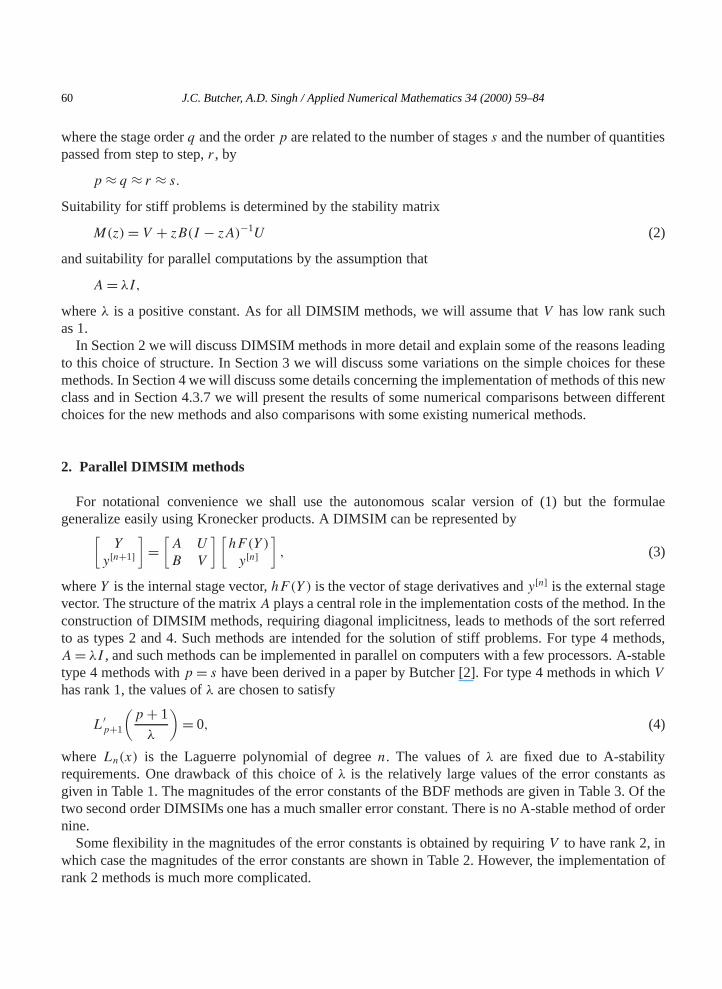
where the stage orderq and the orderp are related to the number of stagess and the number of quantitiespassed from step to step,r , by

p ≈ q ≈ r ≈ s.Suitability for stiff problems is determined by the stability matrix

M(z)= V + zB(I − zA)−1U (2)

and suitability for parallel computations by the assumption that

A= λI,whereλ is a positive constant. As for all DIMSIM methods, we will assume thatV has low rank suchas 1.

In Section 2 we will discuss DIMSIM methods in more detail and explain some of the reasons leadingto this choice of structure. In Section 3 we will discuss some variations on the simple choices for thesemethods. In Section 4 we will discuss some details concerning the implementation of methods of this newclass and in Section 4.3.7 we will present the results of some numerical comparisons between differentchoices for the new methods and also comparisons with some existing numerical methods.

2. Parallel DIMSIM methods

For notational convenience we shall use the autonomous scalar version of (1) but the formulaegeneralize easily using Kronecker products. A DIMSIM can be represented by[

Y

y[n+1]]=[A U

B V

][hF(Y )

y[n]], (3)

whereY is the internal stage vector,hF(Y ) is the vector of stage derivatives andy[n] is the external stagevector. The structure of the matrixA plays a central role in the implementation costs of the method. In theconstruction of DIMSIM methods, requiring diagonal implicitness, leads to methods of the sort referredto as types 2 and 4. Such methods are intended for the solution of stiff problems. For type 4 methods,A= λI , and such methods can be implemented in parallel on computers with a few processors. A-stabletype 4 methods withp = s have been derived in a paper by Butcher [2]. For type 4 methods in whichV

has rank 1, the values ofλ are chosen to satisfy

L′p+1

(p+ 1

λ

)= 0, (4)

whereLn(x) is the Laguerre polynomial of degreen. The values ofλ are fixed due to A-stabilityrequirements. One drawback of this choice ofλ is the relatively large values of the error constants asgiven in Table 1. The magnitudes of the error constants of the BDF methods are given in Table 3. Of thetwo second order DIMSIMs one has a much smaller error constant. There is no A-stable method of ordernine.

Some flexibility in the magnitudes of the error constants is obtained by requiringV to have rank 2, inwhich case the magnitudes of the error constants are shown in Table 2. However, the implementation ofrank 2 methods is much more complicated.

J.C. Butcher, A.D. Singh / Applied Numerical Mathematics 34 (2000) 59–84 61

Table 1Error constants for methods withs = p andV of rank 1

p 1 2 2 3 4 5 6 7 8 10

|Cp+1| 0.5 0.25 4.08 1.03 8.39 2.78 22.98 8.56 71.55 240.06

Table 2Error constants for methods withs = p, V of rank 2and the smallestλ in the stability interval

p 3 4 5 6 7 8

|Cp+1| 0.24 0.45 0.33 0.53 2.21 5.01

Table 3Error constants for BDF methods

p 1 2 3 4 5

|Cp+1| 12

29

322

12125

10137

3. Some implementation details

The implementation of any numerical method requires some basic procedures such as stepsize control,order control if necessary, as well as procedures for the computation of more general quantities such asJacobian and LU factorizations. In this paper we only discuss issues which are specific to our methods.Some of the other issues are discussed in [8].

3.1. Nordsieck representation

An efficient implementation of any numerical method for solving ODEs requires variable stepsize andpossibly variable order. This enables the solver to choose the most appropriate stepsize/order to solve agiven problem at a particular point. One way of implementing type 4 DIMSIMs in a variable stepsizemode is to modify the external stages vectory[n], which hasp components, to the Nordsieck vector,

y[n] = [yn, hy′n, h2y′′n, . . . , hpy(p)n

]T,

with p + 1 components. Hereyn, y′n, y′′n , . . . , y(p)n are approximations toy(xn), y′(xn), y′′(xn), . . . ,y(p)(xn), respectively. This change is achieved by modifying the DIMSIM characterized by (3) whereA,U , B andV are allp× p matrices, to the method characterized by[

Y

y[n+1]]=[A U

B V

][hF(Y )

y[n]], (5)

whereU , B andV , which are of sizesp×p, p×(p+1), (p+1)×p and(p+1)×(p+1), respectively.Then changing stepsize from sayh to ρh, involves rescaling the the Nordsieck vector to

y[n] = [yn, ρhy′n, ρ2h2y′′n, . . . , ρphpy(p)n

]T.

62 J.C. Butcher, A.D. Singh / Applied Numerical Mathematics 34 (2000) 59–84

It is possible to derive these methods characterized by the matricesA, U , B and V directly usingthe order conditions. However, this will not lead to any practical routine for deriving these coefficientsaccurately. The coefficients of the methods characterized by theA, U , B andV matrices can be easilycalculated using the routines based on their derivation as outlined in [2]. Assuming thatA, U , B andVcoefficients are already available, the matricesU , B andV can be derived very easily as shown below.

3.2. DefiningU

We consider the DIMSIMs represented by (3) withU = I andA= λI for the type 4 methods. Fromthe first equation after rearrangement, we have

y[n]i = Yi − λhf (Yi)+O

(hp+1)

= y(xn + cih)− λhy′(xn + cih)+O(hp+1)

= y(xn)+ (ci − λ)hy′(xn)+(c2i

2! − λci)h2y′′(xn)+ · · · +

(cpi

p! − λcp−1i

(p− 1)!)hpy(p)(xn)

+O(hp+1)

for i = 1,2, . . . , s. Putting these equations together gives

y[n] = U y[n], (6)

wherey[n] = [yn, hy′n, . . . , hpy(p)n ]T is the Nordsieck vector. The elements ofU can be obtained as

U =

1 c11

2!c21 . . .

1

p!cp1

1 c21

2!c22 . . .

1

p!cp2

......

......

1 cp1

2!c2p . . .

1

p!cpp

− λ

0 1 c11

2!c21 . . .

1

(p− 1)!cp−11

0 1 c21

2!c22 . . .

1

(p− 1)!cp−12

......

......

...

0 1 cp1

2!c2p . . .

1

(p− 1)!cp−1p

. (7)

Theorem 3.1. When the original DIMSIM method given by(3) with U = I is modified to the form(5),where the output vector is the Nordsieck vector,y[n], then

U B = B, (8)

U V = V U . (9)

Proof. The original method (3) can be written as

Y =AhF(Y )+Uy[n], (10)

y[n+1] = BhF(Y )+ Vy[n], (11)

while the modified method can be written as

Y =AhF(Y )+ U y[n], (12)

y[n+1] = BhF (Y )+ V y[n]. (13)

J.C. Butcher, A.D. Singh / Applied Numerical Mathematics 34 (2000) 59–84 63

Premultiply (13) byU to get

U y[n+1] = UBhF (Y )+ U V y[n] (14)

and using (6) in (11) we get

U y[n+1] = BhF(Y )+ V U y[n]. (15)

By comparing Eqs. (14) and (15) we obtain the result.2We, therefore, need to determine the matricesB andV to satisfy Eqs. (8) and (9). However, the choice

of B andV is not unique in the sense that we can choose the rank of theV matrix. Since the calculationof matricesB and V depend on the rank of theV matrix, we look at these separately in the followingsections.

3.3. Modification to rank 1 methods

3.3.1. Determination ofVSinceV is a rank 1 matrix, we letV = e[v1, v2, . . . , vp]. B and V are interrelated as they need to

satisfy (13). With the choice ofB given in the next section, the(p + 1) × (p + 1) matrix V takes theform

V =

v1 v2 . . . vp+1

0 0 . . . 0...

......

0 0 . . . 0

.We now have

U V = e[v1, v2, . . . , vp+1]

and

V U = e[

p∑i=1

vi,

p∑i=1

vi ui,2,

p∑i=1

viui,3, . . . ,

p∑i=1

viui,p+1

].

Since we haveUV = V U , by equating terms, we get

v1=p∑i=1

vi = 1,

vj =p∑i=1

vi ui,j , j = 2,3, . . . , p+ 1.

Hence, the matrixV can be easily calculated sinceU is known explicitly.

64 J.C. Butcher, A.D. Singh / Applied Numerical Mathematics 34 (2000) 59–84

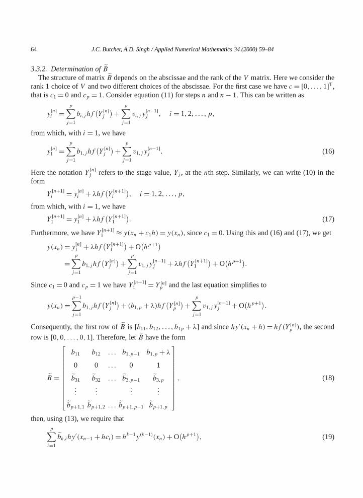
3.3.2. Determination ofBThe structure of matrixB depends on the abscissae and the rank of theV matrix. Here we consider the

rank 1 choice ofV and two different choices of the abscissae. For the first case we havec = [0, . . . ,1]T,that isc1= 0 andcp = 1. Consider equation (11) for stepsn andn− 1. This can be written as

y[n]i =

p∑j=1

bi,j hf(Y[n]j

)+ p∑j=1

vi,j y[n−1]j , i = 1,2, . . . , p,

from which, withi = 1, we have

y[n]1 =

p∑j=1

b1,jhf(Y[n]j

)+ p∑j=1

v1,j y[n−1]j . (16)

Here the notationY [n]j refers to the stage value,Yj , at thenth step. Similarly, we can write (10) in theform

Y[n+1]i = y[n]i + λhf

(Y[n+1]i

), i = 1,2, . . . , p,

from which, withi = 1, we have

Y[n+1]1 = y[n]1 + λhf

(Y[n+1]1

). (17)

Furthermore, we haveY [n+1]1 ≈ y(xn + c1h)= y(xn), sincec1= 0. Using this and (16) and (17), we get

y(xn)= y[n]1 + λhf(Y[n+1]1

)+O(hp+1)

=p∑j=1

b1,jhf(Y[n]j

)+ p∑j=1

v1,j y[n−1]j + λhf (Y [n+1]

1

)+O(hp+1).

Sincec1= 0 andcp = 1 we haveY [n+1]1 = Y [n]p and the last equation simplifies to

y(xn)=p−1∑j=1

b1,jhf(Y[n]j

)+ (b1,p + λ)hf (Y [n]p )+ p∑j=1

v1,j y[n−1]j +O

(hp+1).

Consequently, the first row ofB is [b11, b12, . . . , b1p + λ] and sincehy′(xn + h)= hf (Y [n]p ), the second

row is [0,0, . . . ,0,1]. Therefore, letB have the form

B =

b11 b12 . . . b1,p−1 b1,p + λ0 0 . . . 0 1

b31 b32 . . . b3,p−1 b3,p

......

......

bp+1,1 bp+1,2 . . . bp+1,p−1 bp+1,p

, (18)

then, using (13), we require thatp∑i=1

bk,ihy′(xn−1+ hci)= hk−1y(k−1)(xn)+O

(hp+1), (19)

J.C. Butcher, A.D. Singh / Applied Numerical Mathematics 34 (2000) 59–84 65

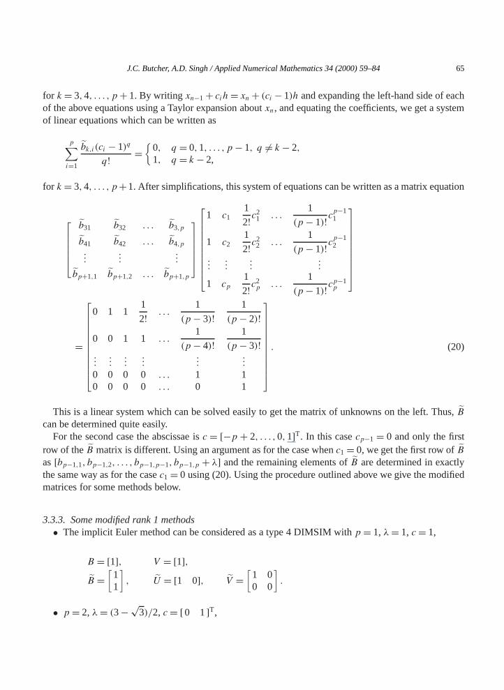
for k = 3,4, . . . , p+ 1. By writing xn−1+ cih= xn+ (ci − 1)h and expanding the left-hand side of eachof the above equations using a Taylor expansion aboutxn, and equating the coefficients, we get a systemof linear equations which can be written as

p∑i=1

bk,i(ci − 1)q

q! ={

0, q = 0,1, . . . , p− 1, q 6= k− 2,1, q = k − 2,

for k = 3,4, . . . , p+1. After simplifications, this system of equations can be written as a matrix equation

b31 b32 . . . b3,p

b41 b42 . . . b4,p...

......

bp+1,1 bp+1,2 . . . bp+1,p

1 c11

2!c21 . . .

1

(p− 1)!cp−11

1 c21

2!c22 . . .

1

(p− 1)!cp−12

......

......

1 cp1

2!c2p . . .

1

(p− 1)!cp−1p

=

0 1 11

2! . . .1

(p− 3)!1

(p− 2)!0 0 1 1 . . .

1

(p− 4)!1

(p− 3)!...

......

......

...

0 0 0 0 . . . 1 10 0 0 0 . . . 0 1

. (20)

This is a linear system which can be solved easily to get the matrix of unknowns on the left. Thus,B

can be determined quite easily.For the second case the abscissae isc = [−p + 2, . . . ,0,1]T. In this casecp−1 = 0 and only the first

row of theB matrix is different. Using an argument as for the case whenc1= 0, we get the first row ofBas[bp−1,1, bp−1,2, . . . , bp−1,p−1, bp−1,p + λ] and the remaining elements ofB are determined in exactlythe same way as for the casec1= 0 using (20). Using the procedure outlined above we give the modifiedmatrices for some methods below.

3.3.3. Some modified rank 1 methods• The implicit Euler method can be considered as a type 4 DIMSIM withp = 1, λ= 1, c= 1,

B = [1], V = [1],B =

[11

], U = [1 0], V =

[1 00 0

].

• p = 2, λ= (3−√3)/2, c= [0 1]T,

66 J.C. Butcher, A.D. Singh / Applied Numerical Mathematics 34 (2000) 59–84

B =

18− 11

√3

4

−12+ 7√

3

422− 13

√3

4

−12+ 9√

3

4

, V =

3− 2√

3

2

−1+ 2√

3

23− 2√

3

2

−1+ 2√

3

2

,

B =

18− 11

√3

4

−6+ 5√

3

40 1−1 1

, U =

1−3+√3

20

1−1+√3

2

−2+√3

2

,

V =

1−4+ 3

√3

2

8− 5√

3

40 0 00 0 0

.• p = 3, λ= 1.21013831273,c = [0 1

2 1]T,

B =

−6.4518297302 14.0277199958 −5.2353370147

0 0 11 −4 34 −8 4

,

U =1 −1.2101383127 0 0

1 −0.7101383127 −0.4800691564 −0.13043395581 −0.2101383127 −0.7101383127 −0.4384024897

,

v =

1 −1.3405532509 −1.2785229832 1.03087017450 0 0 00 0 0 00 0 0 0

.For the case wherep = 3, 4/λ is a zero of the cubic polynomialL′4(x).

3.4. Error estimation for stepsize control in rank 1 methods

In a variable stepsize implementation, in order to control the stepsize we need procedures forestimating the local truncation error,Cp+1h

p+1y(p+1)(xn). The methods used for estimating these errorsdepend on the rank of theV matrix. We first consider estimates for methods withp = s with the Vmatrix of rank 1. It is possible to take various linear combination of stage derivatives of two consecutivesteps, in order to get an estimate ofhp+1y(p+1)(xn). We can either take all the past and present stagevalues or ignore some of these in getting these estimates. Since the components of the Nordsieck vectorare calculated by a linear combination of the stage derivatives in that step, it is also possible to use thesecomponents. This is equivalent to using all the stage derivatives in each step. In the following derivationwe use the notationY [n] to denote the stage valuesY at stepn.

Theorem 3.2. If we use a type4 DIMSIM method of rank1 and orderp, and the stepsize changes fromh/ρ to h, then the local truncation error satisfies

J.C. Butcher, A.D. Singh / Applied Numerical Mathematics 34 (2000) 59–84 67

hp+1y(p+1)(xn)=(

ρp

p+ (ρ − 1)∑pj=1 cj

)(y[n]p+1− ρpy[n−1]

p+1

)+O(hp+2). (21)

Proof. Consider the last component of the external stage vectors of stepsn andn − 1. Matrix V is asparse matrix with only the first row which is nonzero. We therefore have

y[n]p+1− ρpy[n−1]

p+1 =p∑i=1

bp+1,ihf(Y[n]i

)− ρp p∑i=1

bp+1,ih

ρf(Y[n−1]i

)≈

p∑i=1

bp+1,ihy′(xn−1+ cih)− ρp

p∑i=1

bp+1,ih

ρy′(xn−2+ ci h

ρ

)

= hpy(p)(xn + θh)− ρp(h

ρ

)py(p)

(xn−1+ θ h

ρ

)+O

(hp+2)

= hp[y(p)(xn + θh)− y(p)

(xn + h

(−1+ θ

ρ

))]+O

(hp+2)

=(θ

(1− 1

ρ

)+ 1

)h(p+1)y(p+1)(xn)+O

(hp+2).

Since the elements ofB satisfy (19) it is seen thatθ is the coefficient of the next term in the Taylor series,that is,

θ =p∑i=1

bp+1,i(ci − 1)p

p! =p∑i=1

bp+1,icpi

p! − 1, (22)

where the following relationships are satisfied:

p∑i=1

bp+1,icqi = 0, q = 0,1, . . . , p− 2, (23)

p∑i=1

bp+1,icp−1i

(p− 1)! = 1. (24)

We can determine an alternative expression forθ , which does not involvebp+1,i , by considering

p∑i=1

bp+1,i

p∏j=1

(ci − cj )= 0.

By expanding the left-hand side and using (23) we findp∑i=1

bp+1,icpi −

p∑j=1

cj

p∑i=1

bp+1,icp−1i = 0.

Therefore, we havep∑i=1

bp+1,icpi =

p∑j=1

cj

p∑i=1

bp+1,icp−1i ,

68 J.C. Butcher, A.D. Singh / Applied Numerical Mathematics 34 (2000) 59–84

and using (24), we havep∑i=1

bp+1,icpi

p! =p∑j=1

cj

p∑i=1

bp+1,icp−1i

p! =∑pj=1 cj

p.

Substituting this into (22), we obtain

θ =∑pj=1 cj

s− 1, (25)

and

θ

(1− 1

ρ

)+ 1= 1

ρ+(

1− 1

ρ

)∑pj=1 cj

p. (26)

Hence, it is found that

y[n]p+1− ρpy[n−1]

p+1 =(

1

ρ+(

1− 1

ρ

)∑pj=1 cj

p

)hp+1y(p+1)(xn)+O

(hp+2),

from which the result of the theorem follows.2Other linear combinations of the stage derivatives of two consecutive steps can also be used to obtain

estimates ofhp+1y(p+1)(xn). In doing this, we can either use all of the stage derivatives of two consecutivesteps or leave out some of them. In our experiments it was observed that error estimation using all of thestage derivatives of two consecutive steps, as given by (21), gave smoothest error estimates.

3.5. Modification to rank 2 methods

3.5.1. Determination ofVFor rank 2 methods the form of theB matrix is the same as the case for rank 1 methods as given

by (18). However, the contents of theB matrix are chosen in a more complicated way as detailed in thenext section. With this form of matrixB, if V has rank 2 thenV has form

V =

v1,1 v1,2 . . . v1,p−1 v1,p v1,p+1

0 0 . . . 0 0 00 0 . . . 0 v3,p v3,p+1...

......

......

0 0 . . . 0 vp+1,p vp+1,p+1

.

Using Eq. (9), we need to satisfyUV = V U . By multiplying the relevant matrices and equating termswe obtain the elements in the first row of theV matrix as

v1,1=p∑i=1

v1,i = 1,

v1,k =p∑i=1

v1,i ui,k, k = 2,3, . . . , p− 1.

The remaining elements ofV can be determined by solving the equationU V = VU , whereU , V andUare submatrices defined as

J.C. Butcher, A.D. Singh / Applied Numerical Mathematics 34 (2000) 59–84 69

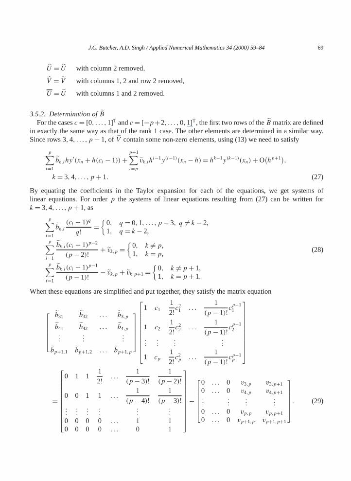
U = U with column 2 removed,

V = V with columns 1, 2 and row 2 removed,

U = U with columns 1 and 2 removed.

3.5.2. Determination ofBFor the casesc= [0, . . . ,1]T andc= [−p+2, . . . ,0,1]T, the first two rows of theB matrix are defined

in exactly the same way as that of the rank 1 case. The other elements are determined in a similar way.Since rows 3,4, . . . , p+ 1, of V contain some non-zero elements, using (13) we need to satisfy

p∑i=1

bk,ihy′(xn + h(ci − 1))+

p+1∑i=p

vk,ihi−1y(i−1)(xn − h)= hk−1y(k−1)(xn)+O

(hp+1),

k = 3,4, . . . , p+ 1. (27)

By equating the coefficients in the Taylor expansion for each of the equations, we get systems oflinear equations. For orderp the systems of linear equations resulting from (27) can be written fork = 3,4, . . . , p+ 1, as

p∑i=1

bk,i(ci − 1)q

q! ={

0, q = 0,1, . . . , p− 3, q 6= k− 2,1, q = k − 2,

p∑i=1

bk,i(ci − 1)p−2

(p− 2)! + vk,p ={

0, k 6= p,1, k = p,

(28)

p∑i=1

bk,i(ci − 1)p−1

(p− 1)! − vk,p + vk,p+1={

0, k 6= p+ 1,1, k = p+ 1.

When these equations are simplified and put together, they satisfy the matrix equation

b31 b32 . . . b3,p

b41 b42 . . . b4,p...

......

bp+1,1 bp+1,2 . . . bp+1,p

1 c11

2!c21 . . .

1

(p− 1)!cp−11

1 c21

2!c22 . . .

1

(p− 1)!cp−12

......

......

1 cp1

2!c2p . . .

1

(p− 1)!cp−1p

=

0 1 11

2! . . .1

(p− 3)!1

(p− 2)!0 0 1 1 . . .

1

(p− 4)!1

(p− 3)!...

......

......

...

0 0 0 0 . . . 1 10 0 0 0 . . . 0 1

−

0 . . . 0 v3,p v3,p+1

0 . . . 0 v4,p v4,p+1...

......

...

0 . . . 0 vp,p vp,p+1

0 . . . 0 vp+1,p vp+1,p+1

. (29)

70 J.C. Butcher, A.D. Singh / Applied Numerical Mathematics 34 (2000) 59–84

Comparing this with the corresponding matrix equation for the rank 1 case, (20), we see that the matrixbeing subtracted here is theV matrix for the rank 2 case, with its first two rows and the first columnremoved. Since the right-hand side is known, this matrix equation can be solved by a linear equationsolver to get the unknown elements inB.

3.5.3. Some modified rank 2 methodsFor L-stability of these methods, the values ofλ lie in an interval as given in [2]. For the methods given

below the smallest values ofλ are used.• p = 3, λ= 0.81,c= [0 1

2 1]T,

B =

0.0718823104 2.5821330578 −0.5973239704

0 0 1−4.1749003488 3.9088099671 0.2660903817−12.6932269318 17.5122902165 −4.8190632847

,

U =1 −0.81 0 0

1 −0.31 −0.28 −0.08041666671 0.19 −0.31 −0.2383333333

,V =

1 −1.0566913978 −0.1937425585 0.14256201960 0 0 00 0 −1.2204953653 0.3783535632

.• p = 4, λ= 1.081,c= [0 1

323 1]T,

B =

3.0648114293 −13.4012626618 19.3782582549 −7.1368070224

0 0 0 1−35.4590194154 98.6708013894 −93.9645445325 30.7527625585−36.4288776113 110.9585864510 −112.6305400681 38.1008312284−74.2097721365 210.0164999157 −197.4036834218 61.5969556427

,

U =

1 −1.0810000000 0 0 01 −0.7476666667 −0.3047777778 −0.0538827160 −0.00615843621 −0.4143333333 −0.4984444444 −0.1908395062 −0.04515226341 −0.0810000000 −0.5810000000 −0.3738333333 −0.1385000000

,

V =

1 −0.9050000000 −0.8149442602 0.1733051580 0.35690732240 0 0 0 00 0 0 1.0229174285 −0.59431502600 0 0 0.8142273759 −0.4730661054

.3.5.4. Error estimation for rank 2 methods

There are a few different ways in which error estimators can be chosen for methods where the matrixV

has rank 2. The following method is equivalent to (21) for rank 1 methods.

Theorem 3.3. If we use a type4 DIMSIM method of rank2 and orderp, and the stepsize changes fromh/ρ to h, then the local truncation error satisfies:

hp+1y(p+1)(xn)= 1

ξ

(y[n]p+1− ρpy[n−1]

p+1

)+O(hp+2), (30)

J.C. Butcher, A.D. Singh / Applied Numerical Mathematics 34 (2000) 59–84 71

where

ξ =(

1− 1

ρ

)(( p∑j=1

cj

)(1− vp+1,p+1)

p−(p−1∑i=1

p∏j=i+1

cicj

)vp+1,p

p(p− 1)

)+ 1

ρ.

Proof. As for rank 1 methods, we have

y[n]p+1− rpy[n−1]

p+1 =(θ

(1− 1

ρ

)+ 1

)hp+1y(p+1)(xn)+O

(hp+2). (31)

When theV matrix is of rank 2, the elements of theB matrix satisfy (27), from which an expression forθ can be obtained by considering the next term in the Taylor series expansion whenk = p+1. This gives

θ =p∑i=1

bp+1,i(ci − 1)p

p! + vp+1,p

2− vp+1,p+1, (32)

where the coefficients satisfy the conditionsp∑i=1

bp+1,icqi = 0, q = 0,1, . . . , p− 3, (33)

p∑i=1

bp+1,icp−2i

(p− 2)! + vp+1,p = 0, (34)

p∑i=1

bp+1,icp−1i

(p− 1)! + vp+1,p+1= 1. (35)

By expanding the first term of (32), and simplifying it using (33)–(35), it can be shown that

θ =p∑i=1

bp+1,icpi

p! − 1. (36)

As for rank 1 methods, we can look for an equivalent expression forθ , by consideringp∑i=1

bp+1,i

p∏j=1

(ci − cj )= 0.

Expand the left-hand side and use (33) to obtainp∑i=1

bp+1,icpi −

(p∑j=1

cj

)p∑i=1

bp+1,icp−1i +

(p−1∑i=1

p∏j=i+1

cicj

)p∑i=1

bp+1,icp−2i = 0.

On rearrangement of this last equation and using (34)–(35), we havep∑i=1

bp+1,icpi =

(p∑j=1

cj

)(1− vp+1,p+1

)(p− 1)! −

(p−1∑i=1

p∏j=i+1

cicj

)vp+1,p(p− 2)!

orp∑i=1

bp+1,icpi

p! =(

p∑j=1

cj

)(1− vp+1,p+1)

p−(p−1∑i=1

p∏j=i+1

cicj

)vp+1,p

p(p− 1).

72 J.C. Butcher, A.D. Singh / Applied Numerical Mathematics 34 (2000) 59–84

Substituting this expression into (36), we obtain

θ =(

p∑j=1

cj

)(1− vp+1,p+1)

p−(p−1∑i=1

p∏j=i+1

cicj

)vp+1,p

p(p− 1)− 1 (37)

and it follows that

ξ = θ(

1− 1

ρ

)+ 1=

(1− 1

ρ

)(( p∑j=1

cj

)(1− vp+1,p+1)

p−(p−1∑i=1

p∏j=i+1

cicj

)vp+1,p

p(p− 1)

)+ 1

ρ,

completing the proof. 2Other error estimators, which take linear combinations of the stage derivatives of two consecutive

steps, can also be used. It can be shown that one such estimator is

hp+1y(p+1)(xn)= η(

p∑i=1

bihf(Y[n]i

)− ρp p∑i=1

bih

rf(Y[n−1]i

))+O(hp+2), (38)

where

η=(

ρp

p+ (ρ − 1)∑pj=1 cj

).

hf (Y[n]i ) and hf (Y [n−1]

i ), i = 1,2, . . . , p, are the internal stages derivatives at stepn and n − 1respectively, from the rank 2 method andbi, i = 1,2, . . . , p, are the weightings which are numericallyequal to the last row of theB matrix of the corresponding rank 1 method, that is,

bi = bp+1,i of the corresponding rank 1 method.

For rank 2 methods (38) was used in the actual implementation because we observed smoother stepsizecontrol using this estimator.

3.6. Error estimates for variable order

When using a method of orderp, we need an estimate of the error,hp+2y(p+2)(xn), in order to estimatethe stepsizeh, that will be used by the method of orderp+1. This error estimate can be calculated usinga difference of error estimates which are used for controlling stepsize. In order to do this, we needtwo such estimates, ofhp+1y(p+1)(xn) and ofhp+1y(p+1)(xn−1), which can be obtained by keeping thestepsize constant for three steps. Thus, we have

hp+1y(p+1)(xn)≈∇hpy(p)n ,

hp+1y(p+1)(xn−1)≈∇hpy(p)n−1

and it follows that

hp+2y(p+2)(xn)≈∇hpy(p)n −∇hpy(p)n−1=∇2hpy(p)n .

Therefore, we have all the ingredients for a successful parallel implementation of type 4 methods.Using the standard stepsize control technique as in [5], the type 4 DIMSIMs were implemented in avariable stepsize, variable order code. It was observed that the choice of abscissae was not critical to

J.C. Butcher, A.D. Singh / Applied Numerical Mathematics 34 (2000) 59–84 73

the performance of the integrator. Although we successfully solved some well known stiff problems,we found that using these the integrator usually took many smaller steps to solve any particular problemwhen compared to VODE or RADAU5. Even if the internal stages are calculated in parallel these methodsare usually much slower.

As stated earlier, these methods have relatively large error constants and we think that this is onereason why they are not very efficient as solvers of stiff initial value problems. In order to make themmore efficient, we consider methods in which the error constants can be made arbitrarily small.

4. Generalizations

In order to construct methods with small error constants we consider two approaches. The first is toallow the diagonal elements of the matrixA of the method to vary and the second approach is to have anadditional stage.

4.1. Methods with differentλ

Type 4 methods are for parallel implementation. However, the diagonal elements of matrixA do notneed to be equal in order to take advantage of parallelism. Making the assumption that they are allequal, simplifies the derivation a great deal, leading to a simple form of the stability polynomial andtransformations which are used to derive the method coefficients. We consider type 4 methods withs = p and in which the matrixA has the generalized form,A= diag{λ1, λ2, . . . , λs}. The implementationof methods of this type will be slightly more complicated than the methods whereA = λI . However,once the method coefficients have been derived, the details of the Nordsieck implementation are verysimilar to the case whereA = λI , except that we need to allow for the different values ofλ. Theparallel computational cost for a method based on this choice of matrixA is not likely to be any higherthan the case where theλ are chosen to be equal. Although each of the stages requires a differentLU

decomposition, these can be computed in parallel along with the stage iterations. Thus the overall parallelcost remains the same. The derivation and analysis of methods whereA takes this more general form ismuch more difficult since the transformations considered earlier do not apply anymore. By using theorder conditions directly in the next section, we see that it is possible to derive methods with smallererror constants.

4.2. A second order method

We use the order conditions as given in [1] to derive a method withp = q = r = s = 2, abscissaec= [0,1]T and

A=[λ1 00 λ2

], B =

[b11 b12

b21 b22

], U =

[1 00 1

], V =

[1− v v

1− v v

].

We substitute the second order approximations

ez = 1+ z+ 12z

2+O(z3),

ecz =[

11+ z+ 1

2z2

]+O

(z3),

74 J.C. Butcher, A.D. Singh / Applied Numerical Mathematics 34 (2000) 59–84

in the first order condition as in [1]. Dropping the terms involving O(z3) fromw= ecz−zAecz, we obtain

w =[

1− zλ1

1+ z(1− λ2)+ z2(12 − λ2)

].

Using this expression forw in the second order condition as in [1], we find

ezw− zBecz − Vw=[

(1− v − λ1v + λ2v− b11− b12)z+ (12 − λ1− 1

2v+ λ2v − b12)z2

(2+ λ1− λ2− v − λ1v + λ2v− b21− b22)z+ (2− 2λ2− 12v + λ2v− b22)z

2

].

Since this is a second order method, the coefficients ofz andz2 should be zero. This gives the expressionsfor the elements of matrixB in terms ofλ1, λ2 andv. For a second order method, the stability polynomialsatisfies

φ(

exp(z), z)= det

(exp(z)I −M(z))=O

(z3),

whereM(z) is given by (2). Using this in a Mathematica program it is found thatλ1 satisfies

λ1= −3+ 8λ2− 5λ22

−2+ 3λ2. (39)

If we put λ1 = λ2 = λ and solve this last equation, we obtainλ= (3±√3)/2, which are precisely thevalues obtained for the second order method withA= λI . Since we require positive values ofλ1 andλ2,the last equation requires that

35 < λ2<

23 or λ2> 1.

The A-stability of a method with stability polynomial,φ(q, z), is equivalent to the statement that theredo not exist complex numbersw andz such that

(i) φ(q, z)= 0,(ii) Re(z)6 0,(iii) |q|> 1.

By the maximum modulus principle, we can replace (ii) by Re(z)= 0. In order to investigate the possiblevalues ofλ2 for A-stability, we can use a recursive argument based on theSchur criterionfor a polynomialhaving all its zeros in the closed unit disc. We recall that a polynomial, all of whose zeros lie within theopen unit disc in the complex plane, is called a Schur polynomial [7]. By a well-known property ofSchur polynomials we can reduce these polynomials to lower order polynomials, which are also Schurpolynomials [7]. Thus, the value ofλ2 needs to be chosen to ensure that the reduced stability polynomialis always positive. In this case the reduced polynomial is a quadratic whose coefficientsa, b andc arepolynomials inλ2. For A-stability we need to ensure that this quadratic is always positive for the chosenvalue ofλ2. The simplest way of doing this is by choosingλ2 such thata > 0, b > 0 andc > 0. Thisgives the following intervals ofλ2 for an A-stable method

0.5740< λ2<23 or 0.6712< λ2< 3.03815.

Consequently, the values ofλ2 which lead to A-stable methods fall in the interval35 < λ2<

23 or 1.0<λ2< 3.03815.

The error constant of the method is given by

C = 2312− 5λ2+ 5

2λ22.

J.C. Butcher, A.D. Singh / Applied Numerical Mathematics 34 (2000) 59–84 75

Values ofλ2 near the zeros of this quadratic will give methods with small error constants. The zerowhich falls in the A-stability interval is about 1.48. Choosingλ2 = 3

2, we get the A-stable method withthe following coefficient matrices.

A=[ 9

10 0

0 32

], B =

[ 6340 −21

4010340 −9

8

], V =

[ 98 −1

898 −1

8

].

This method has an error constant of124 = 0.04167, which is much smaller than the error constants,

0.2484, 4.0817, of the two second order methods in whichA= λI .As the second order method derived above illustrates, it is possible to derive type 4 methods with much

smaller error constants, if we allow the diagonal elements of matrixA to vary. However, the derivationof higher order methods of this type, using the procedure used above, is much more difficult, especiallythe part involving the verification of A-stability, and unless we can find a systematic procedure for thisderivation, it is not practical. Hence, we do not consider higher order methods based on this approach inthis paper.

4.3. Methods withs = p+ 1

We consider the derivation of A-stable type 4 methods in whichA = λI , but λ does not satisfy (4).By not requiring this condition to hold the methods proposed have order one less than the number ofstages. The stage order of such methods can still be equal to the order. We hope to be able to control themagnitude of the error constants by the appropriate choice ofλ.

4.3.1. A first-order method with two stagesConsider a method with coefficient matrices,A= λI , U , B, V , andc = [0,1]T. Using the Nordsieck

vector as the external stage vector, we havew = [1, z]T. Using the order conditions as given in [1] wehave

ecz = zλecz + Uw+O(z2),

ezw = zBecz + V w+O(z2).

Using these we get

U =[

1 −λ1 1− λ

], B =

[b1 b2

1− k k

], V =

[1 v

0 0

],

where

b1+ b2+ v = 1. (40)

Using the stability matrix for the method,

M(z)= V + z

1− λzBU,we obtain

M(∞)= V − BUλ.

76 J.C. Butcher, A.D. Singh / Applied Numerical Mathematics 34 (2000) 59–84

In order to get L-stability we require that the characteristic polynomial

p(q)= det(qI −M(∞))= (1− b2

λ+ b1k

λ2+ b2k

λ2− kλ+ vλ

)+(−2− b1

λ+ b2

λ+ kλ

)q + q2

has a single zero Hence, we set the constant term and the coefficient ofw equal to zero. Solving thesetwo equations forb1 andb2 gives

b1= 2λ− λ2− k − λk + k2− λv,b2= λ2+ λk− k2+ λv,

and adding them together gives

b1+ b2= 2λ− k.Using this equation with (40) and solving forq gives

k =−1+ 2λ+ v.Putting these together we have

B =[

2− 3λ+ λ2− 3v + 2λv + v2 −1+ 3λ− λ2+ 2v − 2λv − v2

2− 2λ− v −1+ 2λ+ v].

Using the Schur criterion we obtain the region of A-stability as

3−√3

26 λ6 3+√3

2. (41)

Whenλ= (3±√3)/2 the method has an error constant equal to zero and reduces to the second ordermethod which has previously been derived by Butcher [2]. The error constant of this new method is givenby

C = 3

2− 3λ+ λ2.

Since this is a positive quadratic with zeros at(3±√3)/2, it is clear that the error constant can be keptsmall by selecting a value ofλ near these zeros but inside the interval (41). The free parameter,v, can bechosen in any way, as it does not affect the size of the error constant. For example, by choosingλ= 3

4,andv = 0, we haveA= λI and the following method:

B =[ 5

161116

12

12

], U =

[1 −3

4

1 14

], V =

[1 0

0 0

],

which has an error constant,C =− 316. With the same value ofλ but v = 1− λ, the method has the same

error constant but theB andV become

B =[

0 34

14

34

], V =

[1 1

4

0 0

].

In this last method, the final internal stage is calculated in exactly the same way as the first external stage,in much the same way as stiffly accurate Runge–Kutta methods in which the final stage is calculatedusing exactly the same coefficients as the output solution.

J.C. Butcher, A.D. Singh / Applied Numerical Mathematics 34 (2000) 59–84 77

Apart from arbitrary choices ofv, as in the above examples, one can choosev to minimize some normof theB matrix. This was investigated using the MATLAB functionfmins after having chosenλ. Usingλ= 7

10 it was found that the value ofv near 0 which minimizes the infinity norm of matrixB is close to− 1

20. Using these the we get

B =[ 189

400231400

1320

720

], V =

[1 − 1

20

0 0

].

This method has an error constant equal to 0.11, a value much smaller than the error constant of theimplicit Euler method. In practice it is expected to perform better than the implicit Euler method, ifthe two stages are computed in parallel. Of course, in serial computation this new method is morecostly because of the extra stage but we do not see this as a disadvantage in a parallel implementa-tion.

4.3.2. Higher order methodsUsing the stability polynomial and the numerical investigation outlined in [2], the intervals ofλ

required for A-stability of the new methods have been determined. These are shown in Table 4. Forp = 8 and forp > 10 there are no A-stable methods.

The intervals forλ have been obtained experimentally and there is some uncertainty about the cut-offvalues. However, from the perspective of getting smaller error constants, we need to choose values ofλ

that are close to the values ofλ for the methods wheres = p, which are given in the final column inTable 4. As the orders increase, the choice ofλ becomes very sensitive to the size of the error constants,since the error constants are polynomials inλ of increasing orders. Table 5 shows a set of choices ofλ andthe corresponding error constants. Hereλ values have been chosen so that the error constants decrease inmagnitude as order increases.

Table 4Intervals ofλ for A-stability

p Interval forλ λ for s = p1

[3−√3

2 , 3+√32

]3±√3

2

2 [0.576,3.833] 1.2101383127

3 [0.875,1.9449] 1.9442883555

4 [1.053,2.665] 1.3012832613

5 [1.052,1.8059] 1.8056866912

6 [1.265,2.290] 1.3521971029

7 [1.211,1.739] 1.7368002358

8 – –

9 [1.548,1.703] 1.6956068006

78 J.C. Butcher, A.D. Singh / Applied Numerical Mathematics 34 (2000) 59–84

Table 5Error constants for methods in whichs = p+ 1

p λ Cp+1

1 0.7 1.1× 10−1

2 1.2 2.1× 10−2

3 1.944 2.2× 10−3

4 1.3012 5.5× 10−4

5 1.80568 2.1× 10−4

6 1.352193 9.9× 10−5

7 1.7368 3.1× 10−5

9 1.6956068 7.3× 10−6

4.3.3. Choice of abscissae and free parametersFor these new methods, the abscissae remains a free parameter just as they do for the methods in which

s = p. Therefore we can choose the abscissae as we like, as long as they are distinct. We have investigatedthree choices in which the abscissae are equally spaced in[0,1], [−1,1] and in[−s + 2,1]. The choiceof the abscissae determines the magnitude of the coefficients. When the abscissae is chosen to be ineach of the three intervals mentioned, the coefficients have the largest magnitude in the first case for anyparticular order. The smallest magnitude of coefficients result in the last case. When these coefficientsbecome very large their use in the solution of an initial value problem will result in rounding errors. Soalthough it is preferable to keep the abscissae inside the integration interval, the resulting methods havevery large coefficients as the order increases. These high order methods will be of no practical use due tothe influence of rounding errors.

It is possible to choose abscissae to be unequally spaced in[0,1], for example, they can be based onthe roots of the shifted Chebyshev polynomials of the second kind, as in [3]. However, we have no reasonto think that this choice will be in any way superior to the equally spaced choice. Hence, we have notconsidered this any further.

The other remaining free parameters arev2, v3, . . . , vs , which come from the first row of matrixV . Wechose thesevi , i = 2, . . . , s, in such a way that we minimize the maximum norm of theB matrix. Weused the MATLAB functionfmins to do this minimization.

After having chosen the abscissae,c, we use the values ofλ listed in Table 5 and the values ofv whichminimizes the coefficients of theB matrix, to derive methods using aMathematicaprogram.

4.3.4. Some examples of methodsAn example of a third order method• p = 3, λ= 1944

1000, c= [0 13

23 1]T,

J.C. Butcher, A.D. Singh / Applied Numerical Mathematics 34 (2000) 59–84 79

B =

77346972523976562500 −120810497847

488281250250790917569

976562500 −42711572199488281250

1440314641953125 −432094392

19531254320943921953125 −142078339

1953125109608131250 −1620684

15625310074331250 −477728

15625

−13464125

41517125 −42642

12514589125

,

U =

1 −243

125 0 0

1 −604375 −1333

2250 − 103110125

1 −479375 −1208

1125 − 387410125

1 −118125 −361

250 −302375

,v = [1 − 3

25 −1925

2950

], b = [−27 81 −81 27].

• p = 3, λ= 19441000, c= [−1 −1

313 1]T ,

B =

144048861771953125000 −45851377281

1953125000490740335311953125000 −15283792427

195312500021101211915625000 −633036357

1562500063303635715625000 −195387119

1562500013741962500 −182691

3125022475762500

160331250

−143191000

452071000 −47457

1000165691000

,

U =

1 −368

125611250 −427

375

1 −854375

15832250 − 1156

10125

1 −604375 −1333

2250 − 103110125

1 −118125 −361

250 −302375

,v = [1 −1

5 −12

310

], b = [−27

8818 −81

8278

].

• p = 3, λ= 19441000, c= [−2 −1 0 1]T,

B =

761244196311718750000 −25571700889

117187500003322795088911718750000 − 3315566963

1171875000025662589346875000 −256625893

1562500025662589315625000 −209750893

46875000132443187500 −101193

62500744362500

148807187500

−1189250

3817250 −4067

2501439250

,

U =

1 −493

125736125 −1958

375

1 −368125

611250 −427

375

1 −243125 0 0

1 −118125 −361

250 −302375

,v = [1 − 1

50 − 110

110

], b = [−1 3 −3 1] .

In an implementation of these methods we need to have these coefficients calculated to the highestpossible precision. We investigate the effect of the choice of the abscissae on computations.

4.3.5. Error estimation for stepsize control for methods withs = p+ 1For these new methods, one can find an estimate ofhp+1y(p+1)(xn)+O(hp+2) within a single step

by taking a linear combination of the stage derivatives in much the same way as the calculation of the

80 J.C. Butcher, A.D. Singh / Applied Numerical Mathematics 34 (2000) 59–84

final component of the external stage vector for methods in whichs = p. For example, for the first ordermethods listed in the previous section, we have

h2y(2)(xn)+O(h3)=−hf (Y1)+ hf (Y2),

and for a second order method with three stages andc= [0, 12,1]T, the error estimator is

h3y(3)(xn)+O(h4)= 4hf (Y1)− 8hf (Y2)+ 4hf (Y3).

Forp = 3 andc= [−1,0,1]T the error estimator becomes

h3y(3)(xn)+O(h4)= hf (Y1)− 2hf (Y2)+ hf (Y3).

For a method of orderp, with s = p+ 1 stages, the error estimator is given by

hp+1y(p+1)(xn)+O(hp+2)= s∑

i=1

bihf (Yi), (42)

where the weightings,bi , are numerically equal to thebs+1,i of the methods in whichs = p and thesamec, and satisfy (20). This procedure for obtaining error estimates is much simpler to implement,as this estimate is available within a single step, unlike the methods withs = p in which one needs tocalculate at least two estimates of the solution before any error estimate can be obtained. Using these errorestimates these methods can be implemented in a variable stepsize code. The other details concerning thevariable stepsize implementation are exactly the same as for methods in whichp = s.

4.3.6. Error estimates for order control for methods withs = p+ 1In order to implement these methods in a variable order code we require an estimate of the higher

order error,hp+2y(p+2)(xn)+O(hp+3). To obtain this estimate we consider the following modification tothe methods which we assume has been implemented using variable stepsize. Let us examine the outputstage vectory[n] = [y(xn), hy′(xn), . . . , hpy(p)(xn)]T for its error terms. Since there ares stages it is moreconvenient to uses instead ofp. Each of the output stages, except the first, can be expressed as

y[n]k = hk−1y(k−1)(xn)+ φkhsy(s)(xn)+O

(hs+1), k = 2,3, . . . , s, (43)

whereφ2, φ3, . . . , φs depend on the abscissae and can be calculated by considering (13) and leaving outthe first equation resulting from this. Since theV matrix has all rows of zeros except the first, we have

s∑i=1

bkihf (Yi)= hk−1y(k−1)(xn)+ φkhsy(s)(xn)+O(hs+1), k = 2,3, . . . , s. (44)

Substitutingf (Yi)= y′(xn−1+ cih) in the last equation and using a Taylor series expansion we obtain

φk =s∑i=1

bk,i(ci − 1)s−1

(s − 1)! , k = 2,3, . . . , s,

where thebk,i satisfy the following conditions fork = 2,3, . . . , s:

s∑i=1

bk,i(ci − 1)q

q! ={

0, q = 0,1, . . . , s − 2, q 6= k− 2,1, q = k − 2.

J.C. Butcher, A.D. Singh / Applied Numerical Mathematics 34 (2000) 59–84 81

Then, if we change stepsize fromh to rh, we want the components of the external stages, (43), tobe rescaled correctly not only for the first term, which is the usual case, but also for the second term,φkh

sy(s)(xn), k = 2,3, . . . , s. This can be done using an estimate forε[n] = hsy(s)(xn) + O(hs+1) andmodifying the appropriate components of the external stage vector toy[n], where we want to obtain

y[n]k = rk−1hk−1y(k−1)(xn)+ φkrshsy(s)(xn)+O

(hs+1), k = 2,3, . . . , s, (45)

using

y[n]k = rk−1y

[n]k + θkε[n] +O

(hs+1), k = 2,3, . . . , s. (46)

Substituting (43) into this last equation and comparing it with (45), we obtain

θk = φk(rs − rk−1), k = 2,3, . . . , s.

Substituting this expression forθk into (45), we obtain

y[n]k = rk−1y

[n]k + φk

(rs − rk−1)ε[n] +O

(hs+1), k = 2,3, . . . , s.

In an implementation of these methods, the external stage vector can either be directly modified as statedby this equation or theB matrix can be modified as outlined below. Using the last equation and

y[n]k =

s∑i=1

bk,ihf (Yi)+O(hs+1), k = 2,3, . . . , s,

ε[n] = hsy(s)(xn)+O(hs+1)= s∑

i=1

bihf (Yi),

wherebi, i = 1,2, . . . , s, are the weights for error estimation, we obtain

y[n]k =

s∑i=1

[rk−1bk,i + φk(rs − rk−1)bi]hf (Yi)+O

(hs+1).

Hence, if we let the modified method be defined usingB, then its elements are defined as

b1,i = b1,i , i = 1,2, . . . , s,

bk,i = rk−1bk,i + φk(rs − rk−1)bi, i = 1,2, . . . , s, k = 2,3, . . . , s.

Example. p = 1, λ= 710, c= [ 0 1]T,

B =[ 189

400231400

1320

720

], U =

[1 − 7

10

1 310

],

V =[

1 − 120

0 0

], b= [−1 1] ,

B =[ 189

400231400

1320r

2 r − 1320r

2

].

82 J.C. Butcher, A.D. Singh / Applied Numerical Mathematics 34 (2000) 59–84

Example. p = 2, λ= 65, c= [ 0 1

2 1]T,

B =

89250 −314

125739250

− 825

1625

1725

215 −52

5315

, U =1 −6

5 0

1 − 710 −19

40

1 −15 − 7

10

,V =

1 15 −6

50 0 00 0 0

, b = [ 4 −8 4] ,

B =

89250 −314

125739250

− 825r

3 1625r

3 r(1− 8

25r2)

r2(1+ 16

5 r)

r2(−4− 32

5 r)

r2(3+ 16

5 r) .

With this modification, we can obtain an estimate ofhp+2y(p+2)(xn)+O(hp+3) by taking the differenceof hp+1y(p+1)(xn) + O(hp+2) and hp+1y(p+1)(xn−1) + O(hp+2) which are obtained from the errorestimates of two consecutive steps with constant stepsizeh. It has been observed that this modificationhas a mild effect on the error estimates for stepsize control.

4.3.7. Numerical verificationIn order to compare the performance of these methods with the some of the well known stiff solvers

we have solved the Ring Modulator problem which is a stiff problem with a dimension of 15 and a fullJacobian. We have also solved the Medical Akzo Nobel problem, which has a dimension 400 and resultsfrom the semi-discretization of a partial differential equation. These test problems are taken from theCWI testset [6]. We have solved these problems using the solvers VODE, RADAU5 and PSIDE. PSIDEis a relatively new parallel implementation of a four stage Radau IIA method [4].

The problems were solved using a variable stepsize, variable order parallel implementation of the type4 DIMSIMs with s = p+1 of orders 1 to 5. Since the abscissae are free parameters we have investigatedthree choices:• DIMSIM E: c= [0,1/(s − 1),2/(s − 2), . . . ,1]T, s > 2,• DIMSIM F: c= [−1,−1+ 2/(s − 1), . . . ,1]T, s > 2,• DIMSIM G: c= [−s + 2,−s + 3, . . . ,0,1]T, s > 2.

For DIMSIM E the abscissae are equally spaced in[0,1], for DIMSIM F they are equally spaced in[−1,1] except for the method of order 1, and for DIMSIM G they are equally spaced in[−s + 2,1].They all share the same method of order one with two stages which has the abscissaec = [0,1]T. Apartfrom the abscissae all the other details are same for these three sets of methods. The CPU times asmeasured by the subroutine DTIME, taken by the different integrators are displayed in Figs. 1 and 2. ForVODE and RADAU5 we measured the sequential CPU times while for PSIDE we measured the parallelCPU times.

The choice of abscissae does not seem to be critical to the performance of these methods. However,from the point of view of minimizing the number of iterations required in solving the stages, the methodwith the abscissae inside the integration interval is a slightly better choice. Another factor which affectsthe computational cost is the starting values for the stage iterations. For sequential methods the convergedvalues for one stage can be used for the starting values for the next stage. However, when the stages arecalculated in parallel, this is not possible. Thus, at the beginning of a step, there is a need for starting

J.C. Butcher, A.D. Singh / Applied Numerical Mathematics 34 (2000) 59–84 83

values for all the stages in that step. The present implementation uses the Nordsieck vector of the paststep for this purpose. The performance of these methods is likely to improve with better stage predictorsthan the current one.

The methods withs = p + 1 performed slightly better than the methods withs = p. Although thetype 4 DIMSIMs can be successfully implemented in parallel, it is apparent from the results that thepresent implementation, for methods withs = p + 1, is not as efficient as the best of the sequentialsolvers; VODE and RADAU5. By measuring the serial and the parallel times for our code we have

Fig. 1. Results for the Ring Modulator problem using DIMSIMs withs = p+ 1.

Fig. 2. Results for the Medical Akzo Nobel problem using DIMSIMs withs = p+ 1.

84 J.C. Butcher, A.D. Singh / Applied Numerical Mathematics 34 (2000) 59–84

obtained speedup factors of up to 2.5. Our variable order code starts the computation with a methodof order one and two stages. The maximum order is set to five with six stages. Thus, the number ofprocessors used can vary from two to six. One of the reasons for the low speedups obtained could bethe relatively high cost of communication between the processors on modern parallel computers withfew processors. The variable order strategy further complicates parallelism. A reduction of order incursa loss of parallelism. Any change of order would incur a massive movement of data between processors.The order change strategy would need to be much more sophisticated so as to take this into account. Toovercome some of these problems would require much more sophisticated parallel coding.

4.4. Concluding remarks and future work

The computational experience gained with these methods suggests that the serial aspects of themethods are working well. For DIMSIMs that have been investigated in this paper, the importantquantities that are used are the error estimates. Some of the error estimation procedures are effectiveand the methods generally converge at the anticipated rates. Although we now have an effective theorder control strategy, there is a need for a more sophisticated strategy which takes into account thecommunication costs between processors when order is varied.

We have investigated methods in which theV matrix has rank 1 or 2 only. Since we have observeda slight performance gain for rank 2 methods, there is a need to investigate methods with higher ranks.Although the standard assumption has been that the number of stagess is equal to orderp, we have alsoinvestigated the cases = p+ 1. There is no reason whys should not even be greater. The generalizationthat the diagonal elements of theA matrix are equal may not necessarily be the best choice. As we havebeen able to derive a second order method of two stages with different diagonal elements, we furtherneed to investigate higher order methods of this type. Thus, there is a long way to go before we can bereally sure which of these large class of methods give the best performance.

The development of efficient software for the solution of ODEs requires many years of experience.Our methods are new and the computational experience gained with them so far is very limited. It ishoped that further computational experience and understanding of these methods, along with a deeperunderstanding of the issues relating to parallel computation, will enable a more efficient implementation.

References

[1] J.C. Butcher, Diagonally-implicit multi-stage integration methods, Appl. Numer. Math. 11 (1993) 347–363.[2] J.C. Butcher, Order and stability of parallel methods for stiff problems, Adv. Comput. Math. 7 (1997) 79–96.[3] J.C. Butcher, P. Chartier, Parallel general linear methods for stiff ordinary differential and differential algebraic

equations, Appl. Numer. Math. 17 (1995) 213–222.[4] J.J.B. de Swart, Parallel software for implicit differential equations, Ph.D. Thesis, CWI, Amsterdam, 1997.[5] E. Hairer, G. Wanner, Solving Ordinary Differential Equations II, Stiff Problems, 2nd revised edition,

Springer, Berlin, 1996.[6] W.M. Lioen, J.J.B. de Swart, W.A. van der Veen, Test set for IVP solvers, http://www.cwi.nl/cwi/projects/

IVPtestset.shtml, 1996.[7] J.J.H. Miller, On the location of zeros of certain classes of polynomials with applications to numerical analysis,

J. Inst. Math. Appl. 8 (1971) 397–406.[8] A.D. Singh, Parallel diagonally implicit multistage integration methods for stiff ordinary differential

equations, Ph.D. Thesis, The University of Auckland, New Zealand, 1999.