Data-parallel polygonization

www.elsevier.com/locate/parco

Parallel Computing 29 (2003) 1381–1401

Data-parallel polygonization q

Erik G. Hoel 1, Hanan Samet *

Department of Computer Science, Institute of Advanced Computer Studies,

Center for Automation Research, University of Maryland, College Park, MD 20742, USA

Received 2 April 2002; accepted 30 May 2003

Abstract

Data-parallel algorithms are presented for polygonizing a collection of line segments rep-

resented by a data-parallel bucket PMR quadtree, a data-parallel R-tree, and a data-parallel

Rþ-tree. Such an operation is useful in a geographic information system (GIS). A sample per-

formance comparison of the three data-parallel structures for this operation is also given.

� 2003 Published by Elsevier B.V.

Keywords: Data-parallel algorithms; Polygonization; Hierarchical spatial data structures; Lines

1. Introduction

Spatial data consists of spatial objects made up of points, lines, regions, rectan-

gles, surfaces, volumes, and even data of higher dimension which includes time.

Examples of spatial data range from locations of cities, rivers, roads, to the areas

that are spanned by counties, states, crop coverages, mountain ranges, etc. Such datais useful in applications in environmental monitoring, space, urban planning, re-

source management, and geographic information systems (GIS) [14,29].

There are many different representations of spatial data, the most prominent be-

ing the quadtree, R-tree, and Rþ-tree (see [26,27] for an overview). There has not

been much research on the use of such representations in a parallel environment.

qThis work was supported in part by the National Science Foundation under grants EIA-99-00268,

EAR-99-05844, IIS-00-86162, and EIA-00-91474 and Los Alamos Scientific Laboratory under Contract

6255U00153Q.*Corresponding author. Tel.: +1-301-405-1755; fax: +1-301-314-9115.

E-mail address: [email protected] (H. Samet).1 Present address: ESRI 380 New York Street Redlands, CA 92373-8100, USA.

0167-8191/$ - see front matter � 2003 Published by Elsevier B.V.

doi:10.1016/j.parco.2003.05.001

mail to: [email protected]

1382 E.G. Hoel, H. Samet / Parallel Computing 29 (2003) 1381–1401

The most notable has been the work of Bestul [3] who considered a number of quad-

tree variants and showed how to construct them, as well as how to conduct a limited

number of operations on data-parallel quadtrees for regions. His approach was con-

ducted under the data-parallel SAM model of computation [3] which is a subset of

the more general scan model [4]. The R-tree research has been limited to the deve-lopment of algorithms for single cpu-multiple parallel disk systems [18], but no work

has been performed on data-parallel R-trees or Rþ-trees.

In this paper we examine the use of data-parallel versions of the quadtree, R-tree,

and Rþ-tree for the polygonization operation. Polygonization is the process of deter-

mining all closed polygons formed by a collection of planar line segments. We iden-

tify each polygon uniquely by the bordering line with the lexicographically minimum

identifier (i.e., line number) and the side on which the polygon borders the line. Poly-

gonization may be performed in a straightforward fashion without relying upon adata-parallel spatial data structure. In essence, the lines could be sorted based upon

their identifier in Oðlog nÞ time. Next, each line, in sorted sequence, would transmit

its endpoint coordinates, line identifier, and current left and right polygon identifiers

to all following lines via a sequence of OðnÞ scan operations. Each line would inde-

pendently be able to determine the identifiers of the left and right polygons. The

drawback of this approach is that it is an OðnÞ operation with a large number of

scans. By employing a data parallel spatial data structure, the number of global scan

operations (i.e., a scan across the entire processor set) may be reduced by, instead,relying upon segmented scans executed in parallel (where each segment consists of

a small number of lines) thereby speeding the computation.

The rest of this paper is organized as follows. Section 2 reviews sequential spatial

data structures. Section 3 presents the data-parallel computation model while Sec-

tion 4 reviews the polygonization process. Sections 5–7 describe how to perform po-

lygonization for the bucket PMR quadtree, the R-tree, and the Rþ-tree. Section 8

contains the results of a small performance study. Concluding remarks are drawn

in Section 9.

2. Sequential spatial data structures

We are interested in representations that are based on spatial occupancy. Spatial

occupancy methods decompose the space from which the data is drawn (e.g., the

two-dimensional space containing the lines) into regions called buckets. They are also

commonly known as bucketing methods. Traditionally, bucketing methods such asthe grid file [23], BANG file [12], LSD trees [16], Buddy trees [31], BV-trees [11],

PK trees [33], etc. have usually been applied to points. In contrast, we are applying

the bucketing methods to the space from which the data is drawn (i.e., two-dimen-

sions in the case of a collection of line segments which is the domain used in the rest

of this paper).

There are four principal approaches to decomposing the space from which the

data is drawn. One approach buckets the data based on the concept of a minimum

bounding (or enclosing) rectangle. In this case, objects are grouped (hopefully by

E.G. Hoel, H. Samet / Parallel Computing 29 (2003) 1381–1401 1383

proximity) into hierarchies, and then stored in another structure such as a B-tree [7].

The R-tree (e.g., [2,15]) is an example of this approach.

The R-tree and its variants are designed to organize a collection of arbitrary spa-

tial objects (most notably two-dimensional rectangles) by representing them as

d-dimensional rectangles. Each node in the tree corresponds to the smallest d-dimen-sional rectangle that encloses its son nodes. Leaf nodes contain pointers to the actual

objects in the database, instead of sons. The objects are represented by the smallest

aligned rectangle containing them.

The basic rules for the formation of an R-tree are very similar to those for a

B-tree. All leaf nodes appear at the same level. Each entry in a leaf node is a 2-tuple

of the form ðR;OÞ such that R is the smallest rectangle that spatially contains object

O. Each entry in a non-leaf node is a 2-tuple of the form ðR; P Þ such that R is the

smallest rectangle that spatially contains the rectangles in the child node pointedat by P . An R-tree of order ðm;MÞ means that each node in the tree, with the excep-

tion of the root, contains between m6 dM=2e and M entries. The root node has at

least two entries unless it is a leaf node.

For example, consider the collection of line segments given in Fig. 1 shown em-

bedded in a 4 · 4 grid. Let M ¼ 3 and m ¼ 2. One possible R-tree for this collection

is given in Fig. 2a. Fig. 2b shows the spatial extent of the bounding rectangles of the

nodes in Fig. 2a, with broken lines denoting the rectangles corresponding to the sub-

trees rooted at the non-leaf nodes. Note that the R-tree is not unique. Its structuredepends heavily on the order in which the individual line segments were inserted into

(and possibly deleted from) the tree.

The drawback of these methods is that they do not result in a disjoint decompo-

sition of space. The problem is that an object is only associated with one bounding

rectangle (e.g., line segment i in Fig. 2 is associated with rectangle R5, yet it passesthrough R1, R2, R4, and R5). In the worst case, this means that when we wish to de-

termine which object is associated with a particular point (e.g., the containing rect-

angle in a rectangle database, or an intersecting line in a line segment database) in

ha

b

e

fi

c

d

g

Fig. 1. Example collection of line segments embedded in a 4 · 4 grid.

R1 R2

R3 R4 R5 R6

a b c i e fg hd

R3R1

R4

R5

R6R2

a b

c

de

f

g h

i

(a) (b)

R0

R0:

R1: R2:

R6:R5:R4:R3:

Fig. 2. (a) R-tree for the collection of line segments in Fig. 1, and (b) the spatial extents of the bounding

rectangles.


the two-dimensional space from which the objects are drawn, we may have to search

the entire database.

The other approaches are based on a decomposition of space into disjoint cells,

which are mapped into buckets. Their common property is that the objects are de-

composed into disjoint subobjects such that each of the subobjects is associated with

a different cell. They differ in the degree of regularity imposed by their underlying

decomposition rules and by the way in which the cells are aggregated. The price paid

for the disjointness is that in order to determine the area covered by a particularobject, we have to retrieve all the cells that it occupies.

The first method based on disjointness partitions the objects into arbitrary dis-

joint subobjects and then groups the subobjects in another structure such as a B-tree.

The partition and the subsequent groupings are such that the bounding rectangles

are disjoint at each level of the structure. The Rþ-tree [32] and the cell tree [13]

are examples of this approach. They differ in the data with which they deal. The

Rþ-tree deals with collections of objects that are bounded by rectangles, while the

cell tree deals with convex polyhedra.The Rþ-tree is an extension of the k-d-B-tree [25]. The Rþ-tree is motivated by a

desire to avoid overlap among the bounding rectangles. Each object is associated

with all the bounding rectangles that it intersects. All bounding rectangles in the tree

(with the exception of the bounding rectangles for the objects at the leaf nodes) are

non-overlapping. 2 The result is that there may be several paths starting at the root

to the same object. This may lead to an increase in the height of the tree. However,

retrieval time is sped up.

Fig. 3 is an example of one possible Rþ-tree for the collection of line segments inFig. 1. This particular tree is of order ð2; 3Þ although in general it is not possible to

guarantee that all nodes will always have a minimum of two entries. In particular,

the expected B-tree performance guarantees are not valid (i.e., pages are not guaran-

teed to be m=M full) unless we are willing to perform very complicated record inser-

2 From a theoretical viewpoint, the bounding rectangles for the objects at the leaf nodes should also be

disjoint. However, this may be impossible (e.g., when the objects are line segments where many line

segments intersect at a point).

R1 R2

R3 R4 R5 R6

d g a b c fh ic

R5R0

R3

R1

R6R4

ab

c

d

e

f

g h

i

(a) (b)

R2

R0:

R1: R2:

R6:R5:R4:R3: h e i i

Fig. 3. (a) Rþ-tree for the collection of line segments in Fig. 1 and (b) the spatial extents of the bounding

rectangles.


tion and deletion procedures. Notice that line segments c and h appear in two differ-ent nodes, while line segment i appears in three different nodes. Ofcourse, other vari-

ants are possible since the Rþ-tree is not unique.

Methods such as the Rþ-tree and the cell tree (as well as the R*-tree [2]) have the

drawback that the decomposition is data-dependent. This means that it is difficult to

perform tasks that require composition of different operations and data sets (e.g.,

set-theoretic operations such as overlay). In contrast, the remaining two methods,

while also yielding a disjoint decomposition, have a greater degree of data-indepen-

dence. They are based on a regular decomposition. The space can be decomposedeither into blocks of uniform size (e.g., the uniform grid [10]) or adapt the decompo-

sition to the distribution of the data (e.g., a quadtree-based approach such as [28]).

In the former case, all the blocks are of the same size (e.g., the 4 · 4 grid in Fig. 1). In

the latter case, the widths of the blocks are restricted to be powers of two, and their

positions are also restricted.

There are a number quadtree-based approaches [27] for storing collections of line

segments. They differ by being either vertex-based [28] or edge-based [21,22]. Their

implementations make use of the same basic data structure. All are built by applyingthe same principle of repeatedly breaking up the collection of vertices and edges (mak-

ing up the collection) into groups of four blocks of equal size (termed brothers) until

obtaining a subset that is sufficiently simple so that it can be organized by some other

data structure. This is achieved by successively weakening the definition of what con-

stitutes a legal block, thereby enabling more information to be stored in each bucket.

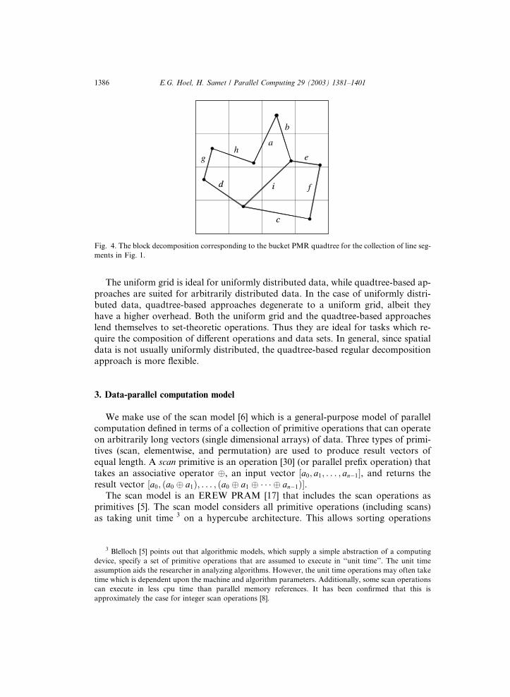
The bucket PMR quadtree [19] is an example of an edge-based quadtree represen-

tation. Each block (or bucket) is split repeatedly until each sub-block contains no

more than b lines, where b is the bucket capacity. For example, Fig. 4 shows theblock decomposition corresponding to the bucket PMR quadtree for the collection

of line segments in Fig. 1 with a bucket capacity 2 and maximal tree height 3. We do

not show the tree representation. There are a total of 10 blocks or buckets with three

of the blocks or buckets being empty. Note that unless the bucket capacity is greater

than or equal to the maximal number of possible intersections, the recursive decom-

position will continue to the maximal depth allowed by the bucket PMR quadtree

(e.g., the endpoints of line segment i in Fig. 4 subdivide until reaching depth 3).

ha

b

e

fi

c

d

g

Fig. 4. The block decomposition corresponding to the bucket PMR quadtree for the collection of line seg-

ments in Fig. 1.


The uniform grid is ideal for uniformly distributed data, while quadtree-based ap-

proaches are suited for arbitrarily distributed data. In the case of uniformly distri-

buted data, quadtree-based approaches degenerate to a uniform grid, albeit they

have a higher overhead. Both the uniform grid and the quadtree-based approaches

lend themselves to set-theoretic operations. Thus they are ideal for tasks which re-

quire the composition of different operations and data sets. In general, since spatial

data is not usually uniformly distributed, the quadtree-based regular decompositionapproach is more flexible.

3. Data-parallel computation model

We make use of the scan model [6] which is a general-purpose model of parallel

computation defined in terms of a collection of primitive operations that can operate

on arbitrarily long vectors (single dimensional arrays) of data. Three types of primi-tives (scan, elementwise, and permutation) are used to produce result vectors of

equal length. A scan primitive is an operation [30] (or parallel prefix operation) that

takes an associative operator �, an input vector ½a0; a1; . . . ; an�1�, and returns the

result vector ½a0; ða0 � a1Þ; . . . ; ða0 � a1 � � � � � an�1Þ�.The scan model is an EREW PRAM [17] that includes the scan operations as

primitives [5]. The scan model considers all primitive operations (including scans)

as taking unit time 3 on a hypercube architecture. This allows sorting operations

3 Blelloch [5] points out that algorithmic models, which supply a simple abstraction of a computing

device, specify a set of primitive operations that are assumed to execute in ‘‘unit time’’. The unit time

assumption aids the researcher in analyzing algorithms. However, the unit time operations may often take

time which is dependent upon the machine and algorithm parameters. Additionally, some scan operations

can execute in less cpu time than parallel memory references. It has been confirmed that this is

approximately the case for integer scan operations [8].


to be performed in Oðlog nÞ time using a simple radix sort. Despite being a general-

purpose model of parallel computation, the scan model has been efficiently imple-

mented on massively parallel processors such as the Thinking Machines CM-2

and CM-5.

Scan operations may be classified in a number of ways. Given a linear ordering ofn processors ½a0; a1; . . . ; an�1�, a scan may be classified as either upward or downward.

An upward scan (also termed a forward scan or a parallel prefix operation), returns

the vector ½a0; ða0 � a1Þ; . . . ; ða0 � a1 � � � � � an�1Þ�. In essence, the ith processor in

the linear ordering receives the result of applying an associative operator to the val-

ues of the preceding i� 1 processors. Analogously, a downward scan (also termed a

backward scan or a parallel suffix operation), returns the vector ½ða0 � a1 � � � ��an�1Þ; ða1 � a2 � � � � � an�1Þ; . . . ; an�1�.

In addition to being classified as either upward or downward, scan operationsmay be segmented or unsegmented. An unsegmented scan is a simple scan across

all processors in the linear ordering. A segmented scan, however, may be thought

of as multiple parallel scans, where each scan operates independently on a segment

of contiguous processors. The segmented groups of processors in the linear ordering

(or segment groups) are commonly delimited by a segment flag, where a value of 1

denotes the first processor in the segment.

Finally, scan operations may be classified as being either inclusive or exclusive.

For example, an upward inclusive scan operation returns the result vector½a0; ða0 � a1Þ; . . . ; ða0 � a1 � � � � � an�1Þ�, while an upward exclusive scan returns the

vector ½0; a0; . . . ; ða0 � a1 � � � � � an�2Þ�.An elementwise primitive is an operation that takes two vectors of equal length

and produces an answer vector, also of equal length. The ith element in the answer

vector is the result of the application of an arithmetic or logical primitive to the ithelements of the input vectors. A permutation primitive takes two vectors, the data

vector and an index vector, and rearranges (permutes) each element of the data vec-

tor to the position specified by the index vector. Note that the permutation must beone-to-one; two or more data elements may not share the same index vector value.

The SAM (scan-and-monotonic-mapping) model [3] is a similar but more restric-

tive model of parallel computation. It makes use of one or more linearly ordered sets

of processors which allow elementwise and scanwise operations to be performed. In

addition, both within and between each linearly ordered set of processors, monotonic

mappings may be performed. A monotonic mapping is defined as one in which the

destination processor indices are a monotonically increasing or monotonically de-

creasing function of the source processor indices. Thus arbitrary permutations arenot allowed in the SAM model. The SAM model affords more efficient hypercube

routing than the standard scan model, thus providing motivation for the more re-

strictive model [3].

The SAM model was useful for the bucket PMR quadtree for which, because of

its regular disjoint decomposition, a unique linear ordering may readily be obtained

(given a particular linear ordering methodology such as a Peano curve [24]). How-

ever, the R-tree and the Rþ-tree, because of their irregular decomposition, do not

have a unique linear ordering thereby necessitating expensive processor reorderings


if we wish to maintain monotonic mappings between their leaf nodes. Thus we ad-

here to the scan model in the rest of this paper.

4. Polygonization

The goal of the polygonization process is to label each line segment with two uni-

que identifiers: one for the polygon on its left and one for the polygon on its right.

The polygons are represented by a partial winged-edge representation [1]. The

winged-edge representation enables us to determine all edges that comprise a poly-

gon in time proportional to the number of edges in the polygon, and all edges that

meet at a vertex in time proportional to the number of edges that are incident at the

vertex. We illustrate our discussion with the aid of Fig. 5. Each line segment z in thecollection is assumed to be directed which means that z has a source and destination

vertex. The partial winged-edge representation contains an association between the

incident line segments at each of the endpoints of z. In particular, there are two poly-

gons associated with each side of z: one on the left and one on the right, where left

and right are with respect to the direction of z. For example, for the polygon on the

left of z, the incoming edge (i.e., at the source vertex) is the one at the minimal angle

formed by the edges incident at the source vertex and z. Similarly, the outgoing edge

(i.e., at the destination vertex) is the one at the maximal angle formed by the edgesincident at the destination vertex and z. On the other hand, for the polygon on the

right of z, the incoming edge (i.e., at the source vertex) is the one at the maximal an-

gle formed by the edges incident at the source vertex and z. Similarly, the outgoing

edge (i.e., at the destination vertex) is the one at the minimal angle formed by the

edges incident at the destination vertex and z.Using Fig. 5 as an example, the left polygon identifier for line segment z is selected

from the minimum identifiers (assuming a lexicographic ordering) of the source end-

point minimal angle (wR, where w is the line identifier and R denotes the right side ofw), the destination endpoint maximal angle (yR), and the line identifier itself (zL). Forthe right polygon identifier, select the minimum identifier among the source endpoint

maximum angle (xR), the destination endpoint minimal angle (vR), and the line iden-

tifier (zR). Therefore, in Fig. 5, line z is assigned wR as the initial left polygon identi-

fier, and vR as the right polygon identifier.

minmax max

min

zw

x

y

v

Fig. 5. Selecting the initial polygon identifiers.


5. Polygonization using the bucket PMR quadtree

The data-parallel PMR quadtree is formed in the same way as the sequential vari-

ants. Given a bucket PMR quadtree, the polygonization process begins by construct-

ing a partial winged-edge representation as described in Section 4. In constructingthe partial winged-edge representation, the endpoints of each line in a node are

broadcast to all other lines in the node through a series of segmented scans. By

broadcast we mean the process of transmitting a constant value from a single proces-

sor to all other processors in the same segment group via a scan operation (i.e., the

vector ½a0; a0; . . . ; a0�). This iterative process is bounded by the maximal number of

lines contained in any node within the quadtree. In most cases, this will equal the

bucket capacity of the quadtree. Locally, each line processor maintains the minimal

and maximal angles formed at each endpoint as well as the identities of the corre-sponding lines. Once the broadcasts are completed, each line processor locally as-

signs an initial polygon identifier to the bordering polygon on the left and right

side (moving from source to destination endpoint).

Next, nodes are merged and duplicate line segments are eliminated. As the dupli-

cated line segments are eliminated, we update the polygon identifiers that are asso-

ciated with their sides to the minimum of the identifiers that are currently associated

with them. For example, if two instances of line z are merged so that the polygon

identifiers associated with the left and right sides of the first instance are aL anddR, respectively, and the polygon identifiers associated with the left and right sides

of the second instance are bL and cR, respectively, then, assuming a lexicographic

minimum, the result is that aL and cR are the polygon identifiers that are now asso-

ciated with the left and right sides of the surviving instance of z. In addition, the up-

date step ensures that all instances of bL and dR are replaced by aL and cR,respectively.

We now show how the polygonization process works for the bucket PMR quad-

tree corresponding to the collection of line segments given in Fig. 1. Fig. 6 shows theinitial polygon assignment for the depicted example where the left and right polygon

identifiers are contained in the LID and RID fields, respectively. The nodes on the left

side of the figure are labeled with numbers corresponding to the order in which they

would be visited by a traversal of the corresponding quadtree in the recursive NW, NE,

SW, and SE order. For each node n in the left side of the figure, we show a pair of

a b

cd

ef

g

h

LID

nodes

lines a f h a b b b ea f a a a b b eL L R L L L L La f a a a b b bR R L R R R R L

RID

1 2 3 4

g c e d f c d gb c c d d c d dR L L L L L L Le c c d d c c cL R R R R R R L

5 6 7 8 9 10

Fig. 6. Initial polygon assignments.

a b

cd

ef

g

h

LID

nodes

lines a f h a b b b ea f a a a b b eL L R L L L L La f a a a b b bR R L R R R R L

RID

1 2 3 4

g c e d f c d gb c c d d c d dR L L L L L L Le c c d d c c cL R R R R R R L

5 6 7

Fig. 7. Result after merging and prior to duplicate deletion.


lines demarcating the set of line segments associated with n. For example, lines a, f ,and h are associated with node 1, while line segments a and b are associated with

node 2. On the other hand, no line segments are associated with nodes 3, 4, and 6.

Starting at the leaf level, sibling nodes are merged together into their parent

nodes. For example, in Fig. 6, leaf nodes 4–7 are merged together, resulting in leaf

node 4 in Fig. 7. All the lines in the merged sibling leaf nodes are sorted, and anyduplicate lines are marked. In Fig. 6, the merging of sibling leaf nodes 4–7 will result

in one pair of duplicate lines (line b) as there is a line b in nodes 5 and 7. The dupli-

cate occurrences of line b are highlighted in Fig. 7 which shows the results of merging

nodes 4–7 prior to duplicate deletion. Duplicate deletion (also known as concentrate

[20]) is accomplished using an upward exclusive scan operation, followed by an ele-

mentwise subtraction, and finally by a permutation operation.

At this point, let us explain the parallel implementation of merging in more detail.

First perform an elementwise operation to tag those nodes that must merge (basedupon tree height). This is followed by a broadcast from the tagged merging nodes

to their corresponding lines telling them they will be merging. Third, perform an up-

ward scan (exclusive, addition) and a permutation to delete the merged nodes (4 sib-

ling nodes become 1 node). Fourth, execute a broadcast operation from nodes to

lines establishing where the node is now located in the linear ordering. Fifth, sort

(via a permutation) the merging lines based upon their line identifiers. Sixth, perform

an elementwise operation to tag the duplicate lines in a node. Seventh, for each set of

duplicate line identifiers (in one merged node), two upward scans (inclusive, seg-mented) are made to update the left and right polygon identifier sets. Eighth, delete

the duplicate lines. Ninth, do a broadcast from the first line in each segment group to

its associated quadtree node.

In order to ensure that each duplicate line has consistent polygon identifiers as

well as correct winged-edge representations, each duplicate line has its endpoints

and polygon identifiers broadcast to the other duplicate lines in the merged node.

If any of the polygon identifiers of the duplicates are updated, then the identifier up-

dates must also then be broadcast among all other lines in the merged nodes. By up-

date, we mean assigning a lexicographically smaller polygon identifier. For instance,

in Fig. 8 the merging of sibling leaf nodes 2–5 will result in two pairs of duplicate

lines (lines b and e) as shown in Fig. 9. For the duplicate occurrence of line b in

the merged node, initially one instance has left and right polygon identifiers aL

a b

cd

ef

g

h

LID

nodes

lines a f h a b b ca f a a a b cL L R L L L La f a a a b cR R L R R R R

RID

1 2 3 4

e e g d f c d ge c b d d c d dL L R L L L L Lb c e d d c c cL R L R R R R R

Fig. 9. Second round of merging prior to duplicate deletion. Duplicate lines b and e in node 2 are shaded.

a b

cd

ef

g

h

LID

nodes

lines a f h a b b ea f a a a b eL L R L L L La f a a a b bR R L R R R L

RID

1 2 3 4

g c e d f c d gb c c d d c d dR L L L L L L Le c c d d c c cL R R R R R R R

5 6 7

Fig. 8. Polygon assignments after the first iteration.


and aR, respectively, while the second instance has left and right polygon identifiers

bL and bR, respectively. The left and right polygon identifiers of the second instanceof line b are updated from bL to aL, and bR to aR, respectively.

If any line has its polygon identifiers updated during the first round of rebroad-

casting, then the polygon identifier update must be communicated in a second round

of broadcasting to all other lines in the merged node. Locally, if the transmitted poly-

gon update matches either the left or right polygon identifiers of the local line, then

the local polygon identifier is updated to reflect the polygon identifiers that have been

broadcast.

For example, consider the situation depicted in Fig. 10 which is taken from themerging nodes shown in Fig. 9. The duplicate occurrences of line b result in two

polygon updates (i.e., bL to aL and bR to aR) being broadcast to the other lines in

a b b c e e g

a a b c b c e

lines

RID

L L L L L L Ra a b c e c bLID

R R R R L R LbL

bR

aL

aR

(a)

eL

cR

cL

aL

(b) (c)

a b b c e e g

a a a c a c eL L L L L L Ra a a c e c a

R R R R L R L

a b b c e e g

a a a a a a cL L L L L L Ra a a c c c a

R R R L L L L

Fig. 10. Updating duplicate line b’s polygon identifier.


the segment group. The other lines whose left or right polygon identifiers are then

updated are shown as circled items in Fig. 10a. Specifically, these are the right poly-

gon identifier of the first occurrence of line e, and the left polygon identifier of line gin the figure. Additionally, the two occurrences of line e also result in two broad-

casted polygon updates (eL to cL and cR to aL) in Fig. 10b. The final result of thebroadcasting of polygon identifiers necessitated by the duplicate occurrence of lines

b and e is shown in Fig. 10c.

When the second instance of line b is updated, the two identifier updates are then

broadcast to all other lines in the merged node. For each other line in the merged

node, if the transmitted polygon identifier update matches either of its current left

or right polygon identifiers, then the line’s polygon identifier is changed to aL in or-

der to reflect the broadcast update and the lexicographically smaller identifier. In the

example, the bL to aL update matches any line whose left or right polygon identifierhave the value bL. Similarly, the two occurrences of line e result in two additional

identifier updates––that is, cR to bL, and eL to cL. Actually, line e’s bL was previouslyupdated to aL during the update broadcasts for line b.

Finally, when merging four sibling nodes together, any line whose endpoint falls

on the shared node border (e.g., lines a and b in Fig. 11a), must also have its end-

points and polygon identifiers broadcast among the merged nodes. for example, con-

sider Fig. 11a where four sibling nodes labeled A–D are being merged. For the sake

of clarity, the contents of nodes C and D are not shown. There are no duplicate linesin the merging nodes, but lines a and b have an endpoint that intersects the common

node border. The endpoint coordinates and polygon identifiers of these two lines are

broadcast among the merged lines, and any appropriate winged-edge updates are

made. In the figure, the source endpoint of line b is updated to reflect the incidence

of line a. For all lines whose winged-edge representations are updated, the polygon

identifiers are checked for possible updates. Fig. 11b shows the resulting polygon

identifiers.

The merging and updating process continues up the entire bucket PMR quadtreeuntil all lines are contained in a single node and all necessary broadcasts have been

made. Fig. 12 depicts the polygon assignments after the second round of leaf node

merging. Fig. 13 shows the result of the final round of merging, prior to duplicate

deletion. In this figure, duplicate lines a, c, d, f , and g are shaded. In this case, line

c’s cR is updated to aL; line d’s dR and cR to aL; line f ’s fR and dR to aL; line f ’s fL and

(a) (b)

ag

c

h

eb

f

daL

aLaLaR

aRaRcL

cL

bL

bR

bL

bL

bR

dR

dR

dR

A B

C D

ag

c

h

eb

f

daL

aLaLaR

aRaRcL

cL

aL

aR

aL

aL

aR

dR

dR

dR

Fig. 11. Example of merging two leaf nodes.

a b

cd

ef

g

h

LID

nodes

lines a a b c c da a a c c dL L L L L La a a a c dR R R L R R

RID

1

d e f f g g hd c f d a d aL L L L R L Rc a f d c c aR L R R L L L

Fig. 13. Final round of merging, prior to duplicate deletion. Duplicate lines a, c, d, f , and g are shaded.

a b

cd

ef

g

h

LID

nodes

lines a f h a b ca f a a a cL L R L L La f a a a aR R L R R L

RID

1 2 3 4

e g d f c d gc a d d c d dL R L L L L La c d d c c cL L R R R R L

Fig. 12. Polygon assignments after the second round of merging.

a b

cd

ef

g

h

LID

nodes

lines a b c d e fa a c a c aL L L R L Ra a a a a aR R L L L L

RID

1

g ha aR Rc aL L

aR cL

aL

Fig. 14. Completion of the polygonization operation.


dL to aR; and line g’s dL and cL to aR and aL, respectively. Finally, Fig. 14 depicts the

completion of the polygonization operation, with the final assigned polygon identi-

fiers circled.

The bucket PMR quadtree’s spatial sort greatly limits the amount of inter-seg-

ment communication necessary as compared with a non-spatially sorted dataset

where all lines would have to communicate their endpoints and polygon identifiers

to all others. In the worse-case, the bucket PMR quadtree polygonization algorithm

has time complexity Oðn log sÞ, where n is the number of lines in the map that cor-responds to a s� s image. However, this is usually not the case as the maximum

number of lines in a segment is really the determinative cost factor and this number

is usually considerably smaller than n. In particular, at each of the Oðlog sÞ stages of


the merging process, the number of scans is proportional to the number of lines in-

tersecting the shared borders of the merging siblings. In the worse-case, all n lines areactive at the final round of merging.

6. Polygonization using the R-tree

The data-parallel R-tree is formed in a different way than the sequential variant.

The difference is that instead of inserting the line segments one-by-one into the data

structure, all line segments are inserted simultaneously. There are a number of ways

of determining the split with differing complexity. The goal is usually one of minimiz-

ing the overlap among the resulting nodes while retaining a certain minimal occu-

pancy level. We do not discuss these issues further here.The polygonization process for the data-parallel R-tree is similar to that described

for the bucket PMR quadtree in Section 5. Given a data-parallel R-tree, we start by

constructing a partial winged-edge representation. Once the partial winged-edge rep-

resentation is completed, each line processor locally assigns an initial polygon iden-

tifier for the bordering polygon on the left and right side (see Section 5 for details).

The initial polygon assignment is shown in Fig. 15 for our example dataset where

the left and right polygon identifiers are contained in processor sets LID and RID, re-

spectively. Next, beginning with the nodes at the leaf level of the R-tree, we merge allsibling lines together into the parent nodes. All lines that intersect any of the over-

lapping regions formed by the bounding boxes of the nodes that have been merged

are marked for rebroadcasting among the lines in the merged nodes. This is neces-

sary in order to propagate the equivalence between the different identifiers in the

merged nodes which represent the same polygon. We do not discuss the merging pro-

cess further here.

For example, consider Fig. 16a where we have two R-tree nodes A and B that are

to be merged. In this example, node A contains lines ða; c; g; hÞ, and node B contains

ab

cd

ef

g

h

LID

N0

lines

N1

N2

45

6 7

2

3

1

f h a b d g c ef f a a d d c cL L L L L L L Lf f a a d d c c

R R R R R R R RRID

4 5 6 7

2 3

1

Fig. 15. Initial polygon assignments.

ag

c

h eb

f

d

aL

aL

aL

aR

aR

aRcL

cL

bL

bR

bL

bL

bR

dR

dR

dR

A

B

(a) (b)

ag

c

h eb

f

d

aL

aL

aL

aR

aR

aRcL

cL

aL

aR

aL

aL

aR

dR

dR

dR

Fig. 16. Two R-tree nodes merging during polygonization.


lines ðb; d; e; f Þ. In the figure, lines ða; b; dÞ must be rebroadcast to the merged set of

lines ða; b; c; d; e; f ; g; hÞ as they intersect the overlapping region formed by thebounding boxes of nodes A and B. The purpose of this operation is to update the

winged-edge representations of any necessary lines. In Fig. 16a, lines a and b require

updating to take place. When the winged-edge representation is updated, we note

any polygon identifiers that must also be updated. In the example in Fig. 16, line

b has both its left and right polygon identifiers updated; bL in Fig. 16a becomes aLin Fig. 16b, and similarly, bR becomes aR. Line a does not have either of its polygon

identifiers updated because its left and right polygon identifiers are lexicographically

minimal.For all such polygon identifier updates (e.g., bL to aL and bR to aR in Fig. 16), we

broadcast the updates to all other lines in the merged node via scan operations. Lo-

cally, if the transmitted polygon update matches either the left or right polygon iden-

tifiers of the local line, then the local polygon identifier is updated to reflect the

polygon identifiers that have been broadcast. For example, in Fig. 16a, the right

polygon identifier of line e is updated to reflect the fact that polygon identifier bR be-

comes aR. Similarly, the left side polygon identifiers of lines d and f are updated to

reflect the fact that polygon identifier bL becomes aL. The resulting polygon identi-fiers and merged nodes are depicted in Fig. 16b. The status of the R-tree polygoniza-

tion operation for Fig. 15 after the first round of leaf node merging is shown in Fig.

17. This process continues up the entire R-tree until all lines are contained in a single

node and all necessary broadcasts have been completed. The final configuration of

our original example dataset is depicted in Fig. 18. Fig. 18 results from merging

nodes 2 and 3 in Fig. 17, and performing the polygon identifier updates. In particu-

lar, the intersection of b and e leads to cR being replaced by aL, the intersection of band g leads to dL being replaced by aR, and the intersection of d and f leads to dRbeing replaced by aL. The identifiers assigned to the three polygons are shown in

the figure by enclosing the identifiers within circles.

The R-tree’s spatial sort greatly limits the amount of inter-segment communica-

tion necessary as compared with a non-spatially sorted dataset where all lines would

have to communicate their endpoints and polygon identifiers to all others. How-

ever, the non-disjoint decomposition of the R-tree causes increased computa-

tional complexities in the local broadcasting phase of the sibling merge operation

ab

cd

ef

g

h

2

3

1

LID

lines

N1

N2

a b f h c d e ga a a a c d c dL L R R L L L La a a a c d c cR R L L R R R L

RID

2 3

1

Fig. 17. Polygonization after first round of leaf node merging.

ab

cd

ef

g

h

1

aR cL

aL

LID

lines

N2

a b c d e f g ha a c a c a a aL L L R L R R Ra a a a a a c aR R L L L L L L

RID

1

Fig. 18. Completion of the polygonization operation.


in comparison to an analogous disjoint decomposition spatial data structure such as

the bucket PMR quadtree or the Rþ-tree (see Section 7). This is because it is often

the case that many lines fall in the intersecting areas when the R-tree nodes aremerged. With representations based on a disjoint decomposition of space, only those

lines that intersect the decomposition lines would need to be locally broadcast during

the sibling merge operation.

Now, let us estimate the number of broadcasts necessary during the polygon iden-

tification process due to the lines intersecting overlapping regions. In the average-

case, assume that each R-tree node has a fan-out of M . Let c (where 06 c6 1) be

the fraction of the lines in each node that intersect one or more of the overlapping

regions formed by the bounding boxes of the nodes that have been merged. Also,let h denote the height of the R-tree; without loss of generality, h ¼ logM n, wheren is the number of lines in the tree. Using the fact that Mh ¼ n, it can be shown that

the number of local broadcasts b that must be made during the merging phases due

to the intersection of lines with the overlapping regions is

b ¼Xh

i¼2

cMi6 n

MM � 1

� �:

This is in the worst-case OðnÞ. However, the average-case complexity is expected to

be lower. In particular, the average-case complexity of the line broadcasting step is


dependent upon the ability of the node splitting algorithm to partition the buckets as

much as possible (therefore lowering the fraction c of lines intersecting the over-

lapping regions).

7. Polygonization using the R+-tree

As in the case of the R-tree, the data-parallel Rþ-tree is formed in a different way

than the sequential variant. Again, the difference is that instead of inserting the line

segments one-by-one into the data structure, all line segments are inserted simulta-

neously with splits being made in accordance with the disjointness requirements as

well as a minimal occupancy level. We do not discuss these issues further here.

The Rþ-tree polygonization algorithm is very similar to that for the R-tree as des-cribed in Section 6. Because the Rþ-tree employs a disjoint decomposition, a single

line may reside in more than one leaf node, similar to the bucket PMR quadtree. In

order to handle this difference with respect to the R-tree, the polygonization algo-

rithm must be changed somewhat during the node-merging phase.

Instead of marking all lines that intersect any of the overlapping regions formed

by the bounding boxes of the nodes that are being merged (as there are none with a

disjoint decomposition), the update procedure follows the technique described for

the bucket PMR quadtree polygonization algorithm in Section 5. All the lines inthe merged sibling node are first sorted according to identifier, and all duplicate lines

are marked for rebroadcasting among the lines in the merged nodes. This enables the

correct updating of duplicate lines in the merged nodes. The duplicate node rebroad-

casting operation is used to update the winged-edge representations of all duplicate

lines and maintain consistency. During the update, we note any polygon identifiers

that must also be updated. Among duplicate lines, if one line has polygon identifiers

that are less than the polygon identifiers of the second line, then this inconsistency

must be resolved, with the smaller identifier taking precedence over the larger. In ad-dition, all lines whose endpoint falls on a common node border are marked for the

rebroadcast of their endpoint coordinates in order to update the winged-edge repre-

sentations and polygon identifiers of any line that may share an endpoint but lie in

another node.

If any line has its polygon identifiers updated during the first round of rebroad-

casting, then the polygon identifier update must be communicated in a second round

of broadcasting to all other lines in the merged node. Locally, if the transmitted poly-

gon update matches either the left or right polygon identifiers of the local line, thenthe local polygon identifier is updated to reflect the polygon identifiers that have been

broadcast. This operation was described in Section 5.

As is the case for the bucket PMR quadtree and R-tree polygonization algo-

rithms, the merging and updating process continues up the entire Rþ-tree until all

lines are contained in a single node and all necessary broadcasts have been made.

The execution time is analyzed in the same manner as that for the bucket PMR

quadtree since the Rþ-tree also makes use of a disjoint decomposition. However,

the merging process is considerably more complex as we need to determine which


of the nodes being merged are adjacent so that we can perform the necessary update

broadcasts.

8. Performance study

Experiments were conducted on a Thinking Machines CM-5 with 32 RISC pro-

cessors and a total of 1 GB of RAM which implies 32 MB per processor. Fig. 20 dis-

plays the execution times for map polygonization for each of the three spatial data

structures using the Prince Georges County map shown in Fig. 19. The Prince

Georges County map contains approximately 35,000 line segments. Due to the per-

Fig. 19. Map of Prince Georges County, Maryland.

50

100

250

500

1000

1500

2000

0 10 20 30 40 50

CPU

Sec

onds

(lo

g sc

ale)

Node Capacity

R+-treeR-tree

bucket PMR quadtree

Fig. 20. Polygonization times for the three structures.


formance inefficiencies of the Rþ-tree, a minimal occupancy level of 49.5% was em-

ployed, while the R-tree used the thirty percent level. From the figure it is clear that

the bucket PMR quadtree offers significant performance advantages over both the

R-tree and the Rþ-tree. The difference is roughly one order of magnitude. It is attri-buted primarily to the considerable amount of time that the R-tree and the Rþ-tree

must spend in determining which nodes are intersecting (or adjoining in the case of

the Rþ-tree) when merging sibling nodes. For the bucket PMR quadtree, this com-

putation is immediate as a result of regular decomposition. In addition, at each stage

of the polygonization process, the R-tree and Rþ-tree merge many more nodes/lines

together; a node occupancy of n implies a fan-out of n. Alternatively, with the bucket

PMR quadtree, four nodes are merged together at each stage of the computation.

Essentially, the bucket PMR quadtree performs a larger number (equal to the heightof the tree) of smaller node merges (with respect to the number of nodes being

merged) than the R-tree and the Rþ-tree.

The fact that the CPU time of the algorithms increases with node capacity,

although slowly, is a result of the need to broadcast the endpoints of each line segment

to all other lines in the node. As we pointed out in Section 5, this process is bounded

by the maximal number of lines in a node. Clearly, modifying the node capacity does

not necessarily prevent a decomposition from taking place which is why the execution

time does not necessarily increase with every incremental increase in node capacity.This is especially true in light of the limited number of data sets that we used.

9. Concluding remarks

Data-parallel algorithms were presented for polygonizing a collection of line seg-

ments represented by a data-parallel bucket PMR quadtree, a data-parallel R-tree,


and a data-parallel Rþ-tree. A sample performance comparison of the three data-

parallel structures showed the data-parallel bucket PMR quadtree to be superior.

Our performance comparison focussed on varying the data structure configurations

(splitting thresholds, node capacities, search radii for range queries, etc.) rather than

on the dataset sizes or the number of processors. Scalability and speedup are direc-tions for future research, as is the implementation of other operations such as spatial

join which is a special case of the join operation [9] where the join condition usually

involves coverage of the same part of space. The spatial join is of interest because it

involves more than one dataset and its performance depends on how well the data

structure can correlate the areas of interest on the different datasets.

References

[1] B.G. Baumgart, Winged-edge polyhedron representation, Artificial Intelligence Laboratory AIM-179,

Stanford University, Stanford, CA, October 1972.

[2] N. Beckmann, H.-P. Kriegel, R. Schneider, B. Seeger, The R*-tree: an efficient and robust access

method for points and rectangles, in: Proceedings of the 1990 ACM SIGMOD International

Conference on Management of Data, Atlantic City, NJ, May 1990, pp. 322–331.

[3] T. Bestul, Parallel Paradigms and Practices for Spatial Data, Ph.D. Thesis, University of Maryland,

College Park, MD, April 1992, also University of Maryland Computer Science Technical Report CS–

TR–2897.

[4] G.E. Blelloch, Scans as primitive parallel operations, IEEE Transactions on Computers 38 (11) (1989)

1526–1538, also Proceedings of the 1987 International Conference on Parallel Processing, St Charles,

IL, August 1987.

[5] G.E. Blelloch, Vector Models for Data-Parallel Computing, MIT Press, Cambridge, MA, 1990.

[6] G.E. Blelloch, J.J. Little, Parallel solutions to geometric problems on the scan model of computation,

in: D.H. Bailey (Ed.), Proceedings of the 1988 International Conference on Parallel Processing, vol. 3,

St Charles, IL, August 1988, pp. 218–222.

[7] D. Comer, The ubiquitous B-tree, ACM Computing Surveys 11 (2) (1979) 121–137.

[8] D. Culler, R. Karp, D. Patterson, A. Sahay, K.E. Schauser, E. Santos, R. Subramonian, T. von

Eicken, Log P : towards a realistic model of parallel computation, in: Proceedings of the Fourth ACM

SIGPLAN Symposium on Principles and Practice of Parallel Programming, San Diego, May 1993,

pp. 1–12.

[9] R. Elmasri, S.B. Navathe, Fundamentals of Database Systems, third ed., Addison-Wesley, Reading,

MA, 2000.

[10] W.R. Franklin, Adaptive grids for geometric operations, Cartographica 21 (2–3) (1984) 160–167.

[11] M. Freeston, A general solution of the n-dimensional B-tree problem, in: Proceedings of the ACM

SIGMOD International Conference on Management of Data, San Jose, CA, May 1995, pp. 80–91.

[12] M.W. Freeston, The BANG file: a new kind of grid file, in: Proceedings of the 1987 ACM SIGMOD

International Conference on Management of Data, San Francisco, May 1987, pp. 287–300.

[13] O. G€uunther, Efficient structures for geometric data management, Ph.D. Thesis, University of

California, Berkeley, CA, 1987, Lecture Notes in Computer Science 337, Springer-Verlag, Berlin,

1988.

[14] R.H. G€uuting, D. Papadias, F.H. Lochovsky (Eds.), Advances in Spatial Databases––Sixth

International Symposium, SSD’99, Hong Kong, July 1999, also Springer-Verlag Lecture Notes in

Computer Science 1651.

[15] A. Guttman, R-trees: a dynamic index structure for spatial searching, in: Proceedings of the 1984

ACM SIGMOD International Conference on Management of Data, Boston, June 1984, pp. 47–

57.


[16] A. Henrich, H.W. Six, P. Widmayer, The LSD tree: spatial access to multidimensional point and non-

point data, in: P.M.G. Apers, G. Wiederhold (Eds.), Proceedings of the Fifteenth International

Conference on Very Large Data Bases, Amsterdam, August 1989, pp. 45–53.

[17] J. J�aaJ�aa, P.Y. Wang, Special issue on data parallel algorithms and programming: guest editors’

introduction, Journal of Parallel and Distributed Computing 21 (1) (1994) 1–3.

[18] I. Kamel, C. Faloutsos, Parallel R-trees, in: Proceedings of the 1992 ACM SIGMOD International

Conference on Management of Data, San Diego, June 1992, pp. 195–204.

[19] M. Lindenbaum, H. Samet, A probabilistic analysis of tree-based sorting of large collections of line

segments, Computer Science Department CS-TR-3455, University of Maryland, College Park, MD,

April 1995.

[20] D. Nassimi, S. Sahni, Data broadcasting in SIMD computers, IEEE Transactions on Computers C 30

(2) (1981) 101–107.

[21] R.C. Nelson, H. Samet, A consistent hierarchical representation for vector data, Computer Graphics

20 (4) (1986) 197–206, also Proceedings of the SIGGRAPH’86 Conference, Dallas, August 1986.

[22] R.C. Nelson, H. Samet, A population analysis for hierarchical data structures, in: Proceedings of the

1987 ACM SIGMOD International Conference on Management of Data, San Francisco, May 1987,

pp. 270–277.

[23] J. Nievergelt, H. Hinterberger, K.C. Sevcik, The grid file: an adaptable symmetric multikey file

structure, ACM Transactions on Database Systems 9 (1) (1984) 38–71.

[24] G. Peano, Sur une courbe qui remplit toute une aire plaine, Mathematische Annalen 36 (1890) 157–

160.

[25] J.T. Robinson. The k-d-B-tree: a search structure for large multidimensional dynamic indexes, in:

Proceedings of the 1981 ACM SIGMOD International Conference on Management of Data, Ann

Arbor, MI, April 1981, pp. 10–18.

[26] H. Samet, Applications of Spatial Data Structures: Computer Graphics, Image Processing, and GIS,

Addison-Wesley, Reading, MA, 1990.

[27] H. Samet, The Design and Analysis of Spatial Data Structures, Addison-Wesley, Reading, MA, 1990.

[28] H. Samet, R.E. Webber, Storing a collection of polygons using quadtrees, ACM Transactions on

Graphics 4 (3) (1985) 182–222, also Proceedings of Computer Vision and Pattern Recognition 83,

Washington DC, June 1983, pp. 127–132, and University of Maryland Computer Science Technical

Report CS–TR–1372.

[29] M. Scholl, A. Voisard (Eds.), Advances in Spatial Databases––Fifth International Symposium,

SSD’97, Berlin, Germany, July 1997, also Springer-Verlag Lecture Notes in Computer Science 1262.

[30] J.T. Schwartz, Ultracomputers, ACM Transactions on Programming Languages and Systems 2 (4)

(1980) 484–521.

[31] B. Seeger, H.-P. Kriegel. The Buddy-tree: an efficient and robust access method for spatial data base

systems, in: D. McLeod, R. Sacks-Davis, H. Schek (Eds.), Proceedings of the Sixteenth International

Conference on Very Large Data Bases, Brisbane, Australia, August 1990, pp. 590–601.

[32] T. Sellis, N. Roussopoulos, C. Faloutsos, The Rþ-tree: a dynamic index for multi-dimensional

objects, in: P.M. Stocker, W. Kent, P. Hammersley (Eds.), Proceedings of the Thirteenth

International Conference on Very Large Data Bases, Brighton, England, September 1987, pp. 507–

518, also University of Maryland Computer Science Technical Report CS–TR–1795.

[33] W. Wang, J. Yang, R. Muntz, PK-tree: a spatial index structure for high dimensional point data, in:

K. Tanaka, S. Ghandeharizadeh (Eds.), Proceedings of the Fifth International Conference on

Foundations of Data Organization and Algorithms (FODO), Kobe, Japan, November 1998, pp. 27–

36.

Data-parallel polygonization

Documents

Transcript of Data-parallel polygonization