Data-Parallel Algorithms for Agent-Based Model Simulation of Tuberculosis OnGraphics Processing Units

Roshan M. D’SouzaDept. of Mechanical EngineeringMichigan Tech. UniversityHoughton, MI, 49931

Email: rmdsouza@mtu.eduSimeone Marino and Denise KirschnerDept. of Immunology and Microbiology

University of MichiganAnn Arbor, MI

Email: simeonem@gmail.com, kirschne@unmich.edu

Keywords: Agent-Based Models, Integrative Systems Biol-ogy,GPGPU

AbstractAgent-based modeling has been recognized as a method tobridge the translational gap in integrative systems biology.However, the computational complexity of agent-based mod-els at biologically relevant scales makes simulation impracti-cal on traditional CPU-based serial computing. In this paperwe present a series of algorithms for simulating large scaleagent-based models on graphics processing units (GPUs).GPUs have recently emerged as a powerful and economicalcomputing platform for certain applications in scientific com-puting. As a test case, we have implemented an agent-basedmodel of tuberculosis. This model simulates the interaction ofthe human immune system in the lung with MycobacteriumTuberculosis and tracks the formation of characteristic struc-ture called garnulomas. The model represents immune cellssuch as T-Cells and Macrophages using mobile agents, effec-tor chemokines using field equations, and bacteria. Our im-plementation is is two orders of magnitude larger and runsthree orders of magnitude faster than the original CPU-basedimplementation.

1. INTRODUCTIONIn the past two decades, there has been much progress

in understanding intra cellular processes. Research in the”omics” fields such as proteomics and genomics has gen-erated vast amount of knowledge. However, this knowledgehas not resulted in many usable clinical therapies. The tra-ditional reductionist approach use in systems biology wherecomplex systems are reduced to a set of linear models has notworked[1]. This is because biological systems are inherentlycoupled, non-linear and heterogeneous. Moreover the under-lying processes span multiple scales in time and space.Increasingly mathematical formulations are being used to

build computer models of these phenomena. Processes suchas diffusion-reaction dynamics of chemicals can be modeledusing deterministic partial differential equations. In case ofinteractions that are intrinsically random, stochastic differen-tial equations are being used[2]. These two approaches arereferred to as equation based modeling as algebraic equationsare used to describe system dynamics. These approaches arevalid if the continuum assumptions hold. For systems wherecontinuum analysis fails due to the paucity in number ofthe molecules, there are stochastic methods such Gillespie’sStochastic Simulation Algorithm (SSA)[3][4]. SSAs have be-come extremely important in characterizing intra-cellular sig-naling events[5][6]. However, all these previous methods arenot suited to the mutli-scale nature of biological systems.

1.1. Agent-BasedModeling in Systems BiologyAgent-based modeling has been recently recognized as

a method to overcome the translational gap in systems bi-ology[7]. Agent-based models(ABM) are direct computa-tional representations of discrete dynamics systems wherethe system level behaviors emerge from the local interac-tion of constituent entities called agents[8]. On a computer,agent are represented as concurrent objects whose state tran-sitions are governed by rules. Agent-based modeling is wellsuited to capture the multi-scale nature of biological sys-tems. ABMs are well suited to capture stochasticity, het-erogeneity, and hierarchy that is present in biological sys-tems. Agent rules can be explicitly derived from the de-scription of biological functions obtained through bench re-search. Unlike equation based modeling, ABMs are descrip-tive and it is easier for biologists with limited mathematicalbackground to relate to this modeling technique. It has beenpreviously used to simulate inflammatory cell tracking[9][10], to model tumor growth[11][12], to simulate intracel-lular processes[13][14][15] bio-molecular reactions, woundhealing[16][17], morphogenesis[18] [19] [20], microvascular

patterning[21], pharmacodynamics[22][23][24][25], tubercu-losis[26], and sepsis[7][27].

1.2. Limitations of Agent-Based ModelingABMs suffer from two major limitations. Due to their

emergent nature, their behaviors cannot be characterized an-alytically. Consequently, techniques for phase plane, bifurca-tion, and stability analysis are non existent[28]. ABMs areto be used in a manner similar to experimentation where sev-eral Monte Carlo runs have to be done to generate statisticallydense data sets[27]. The emergent nature also means that thesystem level behaviors are sensitive to agent populations. Itis therefore required to have representative agent populationsin the model. In systems biology, this can range anywherefrom a few hundred thousand agents to hundreds of millionsof agents.There are several ABM toolkits that have been developed

over the previous two decades[29][30][31]. Most of thesetoolkits provide a set of libraries for canonical agent actionsthat can be extended to implemented model specific agent ac-tions using OOP concepts such as inheritance. These toolk-its are essentially discrete-event simulators[32] that modelagent actions as discrete events. A scheduler queues all theagent actions for a given time step and executes them oneat a time. They are designed to execute serially on the cen-tral processing unit (CPU). Large-scale biological models canhave billions of agent actions for every time step. Such largescale simulations are infeasible on contemporary ABM toolk-its. Parallel computing solutions using computing clusters aremarginally more scalable as compared to single computer im-plementations. Large scale ABM simulation requires entirenew architectures and algorithms.

1.3. ABM Simulation on Graphics ProcessingUnits

GPUs were originally developed to handle computationsrelated to the shaded display of 3D objects. The need fornovel shading effects particularly in video games led ven-dors to enable customized shading through user-defined func-tions that could be programmed directly into hardware. Thisprogrammability enabled computational scientists to use thesame hardware for general purpose scientific computing. Re-cently, the increased use of GPU in scientific computing hasled to the development of specialized computing cards anddirect APIs.GPUs follow the stream programming model[33]. Data is

represented as a stream of elements of the same type. The dataelements could be atomic variables such as integers, floats,characters etc. or user defined complex data structures. Func-tions called kernels mutate the data. In a typical update step,several thousand instances of a single kernel act in parallel ofdifferent elements of the data stream. One major restriction

on the data is that the update of the ith element in the streamis not dependent on the updates of other elements in the sametime step, i.e., there are no precedence constraints. While asmall number of precedence constraints could be handled, astrict ordering of events does not facilitate parallel execution.The main challenege lies in formulating the ABM in terms ofthe stream programming model.

2. PREVIOUS WORKThere are several research efforts related to ABM simu-

lation on the GPU. Harris et al.[34] developed an extensionof Cellular Automata called Coupled Lattice Maps to simu-late boiling, react-diffusion, and convection. Kolb et al. [35]developed a particle simulator implemented almost entirelyon the GPU. For spawning, they used a CPU-based allocator.However, this allocator can be prohibitively time consumingfor large model sizes. Millan and Rudomın[36] developed asystem to simulate crowd behaviors on the GPU. However,their work did not incorporate agent replication and colli-sion avoidance. More recently Perumalla et al. [37] developedan extended cellular automata approach to simulate severalcanonical ABMs on the GPU. While their technique did in-clude collision avoidance, it does not incorporate replication.In addition, mobile agents are bound to lattice sites with amaximum of one agent per site. Richmond et al. [38] haverecently developed techniques to simulated agents in a grid-free environment. Their method is similar to many particlesystems developed previously. However, their agents are ableto communicate with each other in a user-defined radius.The authors previously developed techniques for simulat-

ing large-scale ABMs on GPUs [39]. They demonstrated theirtechniques by implementing a large-scale version of the Sug-arScape ABM. Their incorporated incorporated features suchas environmental resource growth, agent replacement, agentmovement, agent mating, pollution formation, and pollutiondiffusion. They develop a randomized memory allocator thatexecuted entirely on the GPU. In addition, they developed acollision resolution algorithm based on z-culling. This workhas greatly expanded the size and complexity of models thatcan be handled by performing all computations entirely onthe GPU.

3. PAPER OVERVIEWIn this paper we describe our data-parallel implementa-

tion of an ABM to simulate the formation of characteristicstructures called granulomas in the infection pathology ofMycobacterium Tubersculosis (MTb). This model was pre-viously developed by Segovia et al. [26]. The MTb ABMis a discrete-time, discrete-space representation of the com-plex dynamics resulting from the interactions of human im-mune cells with theMTb pathogen in the lung. Mobile agentsare used to represent immune cells such as T-Cells and

Macrophages. The environment represents an section of theaveolar lung tissue. Effects captured in the simulation includeagent motion, chemotaxis, diffusion-decay of chemokines,lysis of bacteria by macrophages, and adaptive immune re-sponse. We begin by briefly describing different elements ofthe MTb ABM. Next, we describe various data-parallel al-gorithms that have been developed to implement the ABM.The results section describe the bench mark studies againsta serial implementation of the same ABM. We conclude thepaper with a discussion of results and future work.

3.1. EnvironmentThe environment in the MTb ABM is modeled using as

a grid of static agents. These agents keep track on the levelof chemokines, bacteria, and the number of mobile immunecells present at each grid location. Chemokine dynamics aremodeled using a linear diffusion decay equation given by:

dEdt

= λ∇2E! γE (1)

where E is the field, λ is the diffusion constant, and γ is the de-cay constant. Infected macrophages act as sources that releasechemokines at the grid point on which they are located at agiven time. Since the chemokines dynamics are two orders ofmagnitude faster than mobile agent dynamics, a quasi staticassumption is used. In between every mobile agent update,the chemokine field is advanced by hundred time steps as-suming stationary agents. Subsequently, the chemokine fieldis updated to account for chemokine release by mobile agentsusing equation given by:

E(t+δt) = E(t)+Cm "δt (2)

where Cm is the chemokine released by an infectedmacrophage per unit time, and δt is the time period of mobileagent update. In the current version of the model, bacteria areseeded at the center of the environment grid. Extra-cellularbacteria grow in the environment according to the equation:

B(t+δt) =min{B(t)+B(t)"αBE(1!B(t)

1.1"KBE),KBE} (3)

where B(t) is the bacteria count at a grid location, αBE isthe bacteria growth rate, KBE is the maximum bacteria countthat can be held at any grid location. In addition, there is aconstraint that any grid cell can contain no more than onemacrophage and one t-cell simultaneously. A randomly cho-sen sub-set of the grid locations act as source compartments.These source compartments model blood vessels and are con-duits for macrophages and t-cells to appear into the simula-tion.

3.2. MacrophagesMacrophages are the most complex of the agent types

in the simulation. Every macrophage is represented us-ing a mobile finite state machine (FSM). The macrophageFSM has five states, namely: RESTING, INFECTED, AC-TIVATED, CHRONICALLY INFECTED, and DEAD. Eachmacrophage has a finite life span. When the enter the sim-ulation, all macrophages are in the RESTING state. In thisstate, they are capable of killing small amounts of extra-cellular bacteria. They can also uptake extra-cellular bacte-ria and become INFECTED. Intra-cellular bacteria BI(t) inINFECTED macrophages grow according to the equation:

BI(t+δt) = B(t)I +BI(t)"αBI (4)

where αBI is the bacteria growth rate. An INFECTEDmacrophage can become ACTIVATED with a small probabil-ity if it encounters a T-Cell in its vicinity. In the ACTIVATEDstate, the macrophage kills all internal and extra-cellular bac-teria it encounters. An INFECTED macrophage can also be-come CHRONICALLY INFECTED if the intra-cellular bac-teria grow and cross a pre-defined threshold. Intracellularbacteria in CHRONICALLY INFECTED macrophage growaccording to:

BI(t+δt) =min{B(t)I +BI(t)"αBI(1!BI(t)KI +30

),KBI} (5)

CHRONICALLY INFECTED macrophages burst when theintra-cellular bacteria reach another threshold KBI andspread the bacteria in the vicinity. CHRONICALLY IN-FECTEDmacrophages can also die if they encounter T-Cells.Macrophages also die when the age exceeds the lifespan.

3.3. T-CellsT-Cells are immune effectors which start appearing in

the simulation on the tenth day of the infection. They havetwo states, namely, LIVE and DEAD. T-Cells move aboutin the environment and perform the task of activating IN-FECTED macrophages and killing CHRONICALLY IN-FECTED macrophages.

3.4. Agent MotionIn the absence of a chemokine field, both T-Cells and

Macrophages perform random motion. In the presence of achemokine field, motion occurs in the direction of the highestgradient. All motion is governed by speed which is depen-dent on the state of the agent. An agent moves to a grid pointif and only if the grid point is not occupied by an agent of thesame type. Otherwise, the agent remains stationary for thattime step. In case the grid point is occupied by another typeof agent, motion occurs with a small probability.

3.5. Cell RecruitmentAt the beginning of the simulation, the environment is

seeded randomly with macrophages. As the simulation pro-ceeds, macrophages and t-cells are recruited from outside theenvironment through the source compartments. Cell recruit-ment occurs only if there is a perceptible chemokine field andthe source compartment is not already occupied by an cell ofthe same type.

4. DATA-PARALLEL TECHNIQUES FORMTB ABM SIMULATION

The main challenge lies in formulating the ABM in termsof stream computation. Model data is to be represented asstream, while as model update function are to be representedas kernels. In our implementation, we use flat arrays to rep-resent model data. Various agent actions such motion, .. areformulated as kernels.

4.1. Data RepresentationThere are five arrays to represent model data. The first

is an array for representing macrophage state data. Themacrophage data structure is given by:

struct Macrophage{position pos; //environment cell location

unsigned int state; // agent statefloat bacteria; //bacteria loadfloat age; //remaining life span};

The second array is for representing T-cell state data. The T-cell data structure is given by:

struct TCell{int x, y; //environment cell locationfloat fx, fy; //actual positionunsigned int state; // agent statefloat age; //remaining life span};

The third array holds the environment state data. The envi-ronment data structure is given by:

struct env{float bacteria;int sourceIndex;}Env[];

Note that the environment data structure does not have spacefor spatial location. Since environment agents are static,

their location is implicitly defined by the location in mem-ory. The variable ”sourceIndex” indicates if the environmentgrid point is a source location and if so, the index of thesource compartment. The value of sourceIndex ranges from 0to MAX SOURCE COMPARTMENTS. Source location areplaces where cell recruitment occurs. The chemokine field isrepresented using a separate array ”E” of floats. This is to fa-cilitate manipulation using Fourier Transforms. Finally, thereare two bit arrays ”Tcmap” and ”Mcmap”, one for resolvingT-Cell collision and the other for resolving Macrophage col-lisions respectively.

4.2. Agent State UpdateAgent state update is accomplished using a set of kernels.

The CPU is used to allocate memory on the GPU for variousagent state arrays as well as to initialize these arrays beforethey are copied to the GPU (left side of figure 1). On the righthand side in figure 1 is the illustration of the order in whichvarious kernels are invoked. In the following sections, each ofthe kernels is described briefly.

Figure 1. Data-parallel simulation loop

4.2.1. Chemokine UpdateAs described previously, the chemokine dynamics are two

orders of magnitude faster than mobile agent dynamics.Therefore, the model requires 100 updates of the chemokinediffusion-decay equation before the mobile agents are up-dated. The application of the diffusion decay kernel on thechemokine field can be thought of as a convolution given by:

E(i, j) =m

∑l=0

m

∑k=0

f (i! k, j! l)E(k, l) (6)

The size of f is a function of the number of time steps m.The overall complexity of this operation is given byO(m2n2),where n is the width of the chemokine field. Ifm<< n, then itis best to do a direct convolution. However, for large m, com-puting this convolution in the Fourier Domain improves thecomplexity to O(m2log(m)+ n2log(n)). Computation in the

Fourier domain is possible because the governing equation islinear time-invariant and the domain has periodic boundaryconditions. At the beginning of the simulation, the diffusion-decay kernel for 100 time steps in the spatial domain is com-puted on the CPU. It is then transferred to the GPU and theFFT is computed and stored on the GPU. Algorithm 3 illus-trates this procedure. f is the FFT of the convolution kernelf .

Algorithm 1 Computer Diffusion Decay Kernel1: procedure compute-diffusion-decay-kernel()2: On the CPU3: f # compute time domain kernel for 100 times steps4: Transfer f to the GPU5: f # FFT( f )

Algorithm 3 illustrates the procedure to update thechemokine field in the Fourier domain. This procedure is runalong with the mobile agent update. This essentially elimi-nates the ”stiffness” associated with the fast chemokine dy-namics. Lines 2-4 solve the diffusion decay equation in thefrequency domain. Lines 6-9 account for chemokine releaseby INFECTED, CHRONICALLY INFECTED, and ACTIVEmacrophages.

Algorithm 2 Update Chemokine Field1: procedure update-chemokine-field(E,M)2: E(t) # FFT(E)3: E(t+δt) # f " E(t)4: E(t+δt) # invFFT(E(t+δt))5: for all m $M in parallel do6: loc# find loc(m.pos)7: if m.state == INFECTED OR CHRONICALLY IN-

FECTED OR ACTIVATED then8: E[loc]+ =CI9: end if10: end for

4.2.2. Environment KernelThe environment kernel is the simplest. It only handles

extra-cellular bacteria growth according to equation . Algo-rithm 1 illustrates the pseudo-code for environment updates.

Algorithm 3 Calculating Extra-Cellular Bacteria Growth1: procedure update-extra-cellular-bacteria(Env)2: for all e $ Env in parallel do3: b# e.bacteria4: b#min{b+b"αBE(1! b

1.1"KBE ),KBE}5: e.bacteria# b6: end for

4.2.3. Macrophage Update

Macrophages are the most complicated agents in the MTbABM. The behaviors of the macrophages are determined bythe agent state. Each of the agent states has different behav-ioral rules. The variable ID is the index of the macrophage inthe array M. It is implicitly calculated by the thread of exe-cution. The main kernel function listed in Algorithm 4 firstaccounts macrophage death due to aging (lines 4-8). Line 9handles agent motion. Next based on the current state of themacrophage, different sub-kernels are called (lines 10-22).

Algorithm 4 Update Macrophages1: procedure update-macrophages(M)2: for all m $M in parallel do3: ID# threadID4: m.age# m.age-Δt5: if m.age < 0 then6: m.state = DEAD7: return8: end if9: update position(ID,m.speed,m.pos,Mcmap)10: if m.state == RESTING then11: restingRules(m)12: end if13: if m.state == INFECTED then14: infectedRules(m)15: end if16: if m.state == CHRONICALLY INFECTED then17: chronicallyInfectedRules(m)18: end if19: if m.state == ACTIVATED then20: activatedRules(m)21: end if22: end for

Algorithm 5 accounts for RESTING behaviors. If themacrophage is at an environment grid where there is sufficientbacteria (NRK , with a small probability pk it can get infected.During infection, it uptakes Nrk amount of bacteria. Its speedalso changes (lines 5-10).

Algorithm 5 Resting Rules1: procedure restingRules(m)2: loc# find loc(m.pos)3: bac# Env[loc].bacteria4: r# rand[0,1]5: if bac > Nrk then6: bac# max(bac-Nrk, 0)7: if r < pk then8: m.bacteria = Nrk9: m.state = INFECTED10: m.speed = INFECTED SPEED11: else12: return13: end if14: end if

Algorithm 6 accounts for INFECTED behaviors. Infectedmacrophages grow intra-cellular bacteria (line 2). Lines 3-6implement state change to CHRONICALLY INFECTED ifthe intra-cellular bacteria grow beyond a threshold Nc. Lines8-14 handle macrophage activation by T-Cells in the Mooreneighborhood.

Algorithm 6 Infected Rules1: procedure infectedRules(m)2: m.bacteria = m.bactera *(1+αBI)3: if m.bacteria > Nc then4: m.state = CHRONICALLY INFECTED5: m.speed = CHRONICALLY INFECTED SPEED6: return7: end if8: n# number of T-Cells in the Moore neighborhood9: r# rand[0,1]10: if r < n" tactm then11: m.state = ACTIVATED12: m.bacteria = 0.013: m.speed = ACTIVATED SPEED14: end if

Algorithm 7 accounts for CHRONICALLY INFECTEDbehaviors. Line 2-4 handle intra-cellular bacteria growth.Lines 5-10 handle the case where the intra-cellular bacteriaload is less than a threshold KBI and the macrophage is killedby a T-Cell. Lines 14-16 handle the case where macrophagesdie because of bacteria overload.

Algorithm 7 Chronically Infected Rules1: procedure chronicallyInfectedRules(m)2: bac# m.bacteria3: bac = min{ bac+ bac*αBI (1- bac

KI+30 ), KBI}4: m.bactera# bac5: if bac < KBI then6: n # min number of T-Cells in the Moore neighbor-

hood7: r# rand[0,1]8: if n> 0 AND r < pTk then9: m.bacteria *= 0.510: burst(m)11: else12: return13: end if14: else15: burst(m)16: end if

Algorithm 8 handles macrophage death. When amacrophage dies, the intra-cellular bacteria load is evenlydistributed between the environment cells in the Mooreneighborhood (lines 2-5).

Algorithm 8 Killing Macrophages1: procedure burst(m)2: for p $Moore neighborhood of m.pos do3: loc# find loc(p)4: Env[loc].bacteria += m.bacteria/9.0f5: end for6: m.state = DEAD7: return

4.2.4. T-Cell UpdateThe T-Cell update is much simpler compared to

macrophages. In the current model, T-Cells have just twostates, namely, LIVE, and DEAD. The T-Cell update kernelincrements the age of the kernel and calls the motion sub-kernel. The motion sub-kernel for the T-Cells is the same asthat of macrophages.

Algorithm 9 Updating T-Cells1: procedure update T-Cells() FOR all t $ T in parallel2: ID# threadID3: t.age# t.age-Δt4: if t.age < 0 then5: t.state = DEAD6: return7: end if8: update position(ID,t.speed,t.pos,Tcmap)

4.2.5. Handling MotionBoth T-Cells and Macrophages move about in the environ-

ment. While T-Cells have a single speed, macrophage speedchanges based on the state. Additionally, the motion is con-strained by the fact that no two cells of the same type can beco-located at the same grid location. Algorithm.. illustratesmotion handling. The input arguments include speed, the po-sition p, and the collision map array. The arrays Deltap con-tain possible motion vectors. The variable ”loc” is an indexinto the chemokine and collision map array corresponding tothe location of the agent. Lines 5-7 select a random motiondirection if the chemokine level at the given location is lessthan the threshold Ethresh. Lines 10,11 generates the possiblenew location and index. If the new index is the same as theold, only the position is updated. If the new index already hasan agent that the motion is rejected. Lines 19-22 handle theconflict if more than one agent try to move to the same lo-cation. We use the atomic compare and swap functionality toaccomplish collision resolution. The variable

Algorithm 10 Handling Agent Motion1: procedure update-position(ID,speed,p,collisionMap)2: loc# find loc(p)3: Δp[] # array of unit vectors to moore neigbhorhood4: e# E[loc]5: if e< Ethresh then6: k# rand[0,8]7: else8: k# direction of maximum chemokine gradient9: end if10: pnew # p+Δp[k]*speed11: new loc# find loc(pnew)12: if collisionMap[loc] == OCCUPIED then13: return14: end if15: if loc == old loc then16: p# pnew17: return18: end if19: if atomicCAS(collisionMap[loc],EMPTY,ID) ==

EMPTY then20: collisionMap[old loc]# EMPTY21: p# pnew22: end if

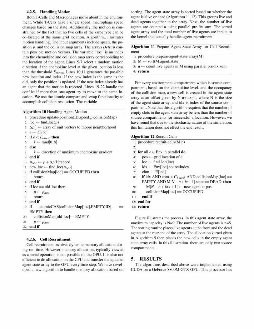
4.2.6. Cell RecruitmentCell recruitment involves dynamic memory allocation dur-

ing run-time. However, memory allocation, typically viewedas a serial operation is not possible on the GPU. It is also notefficient to do allocation on the CPU and transfer the updatedagent state array to the GPU every time step. We have devel-oped a new algorithm to handle memory allocation based on

sorting. The agent state array is sorted based on whether theagent is alive or dead (Algorithm 11,12). This groups live anddead agents together in the array. Next, the number of liveagents are counted n using parallel pre-fix sum. The sortedagent array and the total number of live agents are inputs tothe kernel that actually handles agent recruitment

Algorithm 11 Prepare Agent State Array for Cell Recruit-ment1: procedure prepare-agent-state-array(M)2: M# sort(M,agent state)3: n# count live agents in M using parallel pre-fix sum4: return

For every environment compartment which is source com-partment, based on the chemokine level, and the occupancyof the collision map, a new cell is created in the agent statearray at an offset given by N-n+idx+1, where N is the sizeof the agent state array, and idx is index of the source com-partment. Note that this algorithm requires that the number ofempty slots in the agent state array be less than the number ofsource compartments for successful allocation. However, wehave found that due to the stochastic nature of the simulation,this limitation does not effect the end result.

Algorithm 12 Recruit Cells1: procedure recruit-cells(M,n)2:3: for all e $ Env in parallel do4: pos# grid location of e5: loc# find loc(loc)6: idx# Env[loc].sourceIndex7: chm# E[loc]8: if idx AND chm >CThresh AND collisionMap[loc] ==

EMPTYANDM[N!n+ ix+1].state == DEAD then9: M[N!n+ idx+1] # new agent at pos10: collisionMap[loc] == OCCUPIED11: end if12: end for13: return

Figure illustrates the process. In this agent state array, themaximum capacity is N=9. The number of live agents is n=5.The sorting routine places live agents at the front and the deadagents at the rear end of the array. The allocation kernel givenin Algorithm 5 then places the new cells in the empty agentstate array cells. In this illustration, there are only two sourcecompartments.

5. RESULTSThe algorithms described above were implemented using

CUDA on a GeForce 8800M GTX GPU. This processor has

Figure 2. Parallel memory allocation for cell recruitment

Figure 3. Screen shot of simulation. In this figure, green pix-els represent resting macrophages, orange pixels represent in-fected macrophages, red pixels represent chronically infectedmacrophages, and purple pixels represent T-Cells. All thesecells are chemotactically moving towards the center whereinfected macrophages are releasing chemokines.

96 core and has 360 GFlops processing rate. The GPU imple-mentation was benchmarked against a CPU implementationrunning on a Intel Centrino processor. For the purpose of thebenchmarks, the simulation was run to account for 4 days ofreal time with T-Cells arriving at the begining of the secondday. Figure 1 show the performance scaling with respect tothe increase in the environment size. It is clear that time forsimulation for the GPU implementation barely changes. Ata environment resolution of 256x256, the GPU implementa-tion is .. faster than the CPU implementation. Figure 2 shows

Figure 4. Performance scaling with environment size. Theinitial macrophage population is set to 100. The simulation isrun for 4 days worth of updates with T-Cells being recruitedon the 2nd day

Figure 5. Perfomance scaling with initial macrophage pop-ulation. The environment size is set to 128x128

the scaling with the number of initial macrophages. The envi-ronment resolution for this benchmark was set to 100x100. Itis apparent that the performance for both the CPU and GPUdoes not degrade much in the ranges that we tested. Heretoo, the GPU performance is much better. This clearly indi-cates that most of the computational load is due to the cal-culation of the diffusion decay equation in the environment.Our implementation on the GPU has two advantages. First,the multi-core GPU provides much better computing poweras compared to the CPU. Second, and more importantly, theuse of spectral methods(FFT) for solving the diffusion de-cay equation provides an enhanced speed up due to the sizeof the diffusion decay kernel. Figure shows the comparrisonbetween the output of the two implementations for the sameinitial parameters. Here we track the amount of intra-cellularbacteria over time. The two curves were generated by aver-aging the results of 5 simulation runs. Clearly, the output ofboth simulation show the same trend.

Figure 6. Tracking intra-cellular bacteria with respect totime for the CPU implementation and the GPU implemen-tation. The simulation is run for 15 days with T-Cells beingrecruited on the 10th day. The environment is set to 128x128with initial macrophage population set to 100.

6. CONCLUSIONSWe have successfully developed and implemented a se-

ries of data-parallel algorithms for simulating the Mycobac-terium Tuberculosis ABM. Key innovation that have madethis possible include the collision handling algorithm basedon atomic compare and swap, and the parallel memory allo-cation algorithm based on sorting. Our implementation exe-cutes entirely on the GPU with no communication with theCPU and therefore avoids the bottleneck posed by the slowerCPU-GPU memory bus. Our current simulation only mod-els the dynamics of MTb in the lung. The perfomance gainsobtained through data-parallel execution opens up the pos-sibility of scaling ABMs to realistic levels. We are workingon building an extended model that will include other organssuch as lymphnodes that are involved in the pathology. Ourultimate goal is to build the complete organs system modelwith each organ modeled as a separate ABM with intercon-nects that will model the lymphatic and circulatory system.This model will then be used to virtually test drug protocols.

BiographyREFERENCES[1] Y Vodovotz, M Csete, J Bartels, S Chang, and G An.

Translational systems biology of inflammation. PLoSComputational Biology, 4(4):1–6, 2008.

[2] Bernt Oksendahl. Stochastic differential equations: anintroduction with applications. Springer - Verlag, 2002.

[3] D T Gillespie. General method for numerically simu-lating the stochastic time evolution of coupled chemicalreactions. J. Comput. Phys., 22:403–434, 1976.

[4] D T Gillespie. Exact stochastic simulation of coupledchemical reactions. J. Phy. Chem., 81:2340–2361, 1977.

[5] Quan Liu and Ya Jia. Fluctuations-induced switch inthe gene transcriptional regulatory system. Phys. Rev.E, 70(4):041907, Oct 2004.

[6] Mukund Thattai and Alexander van Oudenaarden.Stochastic gene expression in fluctuating environments.Genetics, 167:523–530, 2004.

[7] G An. Agent-based computer simulation and sirs: build-ing a bridge between basic science and clinical trials.Shock, 16(4):266–273, 2001.

[8] E Boanbeau. Agent-based modeling: methods and tech-niques to simulate human systems. PNAS, 99(3):7280–7287, 2002.

[9] A M Bailey, B C Thorne, and S M Peirce. Multi-cellagent-based simulation of the microvasculature to studythe dynamics of circulating inflammatory cell traffick-ing. Ann. Biomed. Engg., 35(6):916–936, 2007.

[10] J Tang and et al. Simulating leukocyte-venuleinteractions–a novel agent-oriented approach. In Conf.Proc. IEEE Eng. Med. Biol. Soc., volume 7, pages4978–4981, 2004.

[11] L Zhang, C A Athale, and T S Deisboeck. Develop-ment of a three-dimensional multiscale agent-based tu-mor model: simulating gene-protien interaction profiles,cell phenotypes and multicellular patterns in brain can-cer. J. Theor. Biology, 244(1):96–107, 2007.

[12] T S Deisboeck and et al. Pattern of self-organization intumour systems: complex growth dynamics in a novelbrain tumour spheroid model. Cell Prolif., 34(2):115–134, 2001.

[13] D YWong, A Qutub, and C A Hunt. Modeling transportkinetics with starlogo. In Conf. Proc. IEEE Eng. Med.Biol. Soc., volume 2, pages 845–848, 2004.

[14] G Broderick, M Ruaini, E Chan, and M J Ellison. Alife-like virtual cell membrane using discrete automata.In Silico Biol., 5(2):163–178, 2005.

[15] M Pogson, R Smallwood, E Owarnstrom, and M Hol-combe. Formal agent-based modelling of intracellularchemical interactions. Biosystems, 85(1):37–45, 2006.

[16] D C Walker. Agent-based computational modelingof wounded epithelial cell monolayers. IEEE Trans.Nanobioscience, 3(3):153–163, 2004.

[17] Q Mi, B Riviere, G Clermont, D L Steed, andY Vodovotz. Agent-based model of inflammation andwound healing: insights into diabetic foot ulcer pathol-ogy and the role of transforming growth factor-beta1.Wound Repair Regen., 15(5):671–682, 2007.

[18] D Longo, S M Peirce, T C Skalak, L Davidson,M. Marsden, B Dzamba, and DWDeSimone. Multicel-lular computer simulation of morphogenesis: blastocoelroof thinning and matrix assembly in xenopus laevis.Dev. Biol., 271(1):210–222, 2004.

[19] M R Grant, S H Kim, and C A Hunt. Simulatingin vitro epithelial morphogenesis in multiple environ-ments. In Comput. Syst. Bioinformatics Conf., pages381–384, 2006.

[20] S Chen, S Ganguli, and C A Hunt. An agent-based com-putational approach for representing aspects of in vitromulti-cellular tumor spheroid growth. In Conf. Proc.IEEE Eng. Med. Biol. Soc., volume 1, pages 691–694,2004.

[21] S M Peirce, E J van Gieson, and T C Skalak. Multicellu-lar simulation predicts microvascular patterning and in-silico tissue assembly. FASEB J., 18(6):731–733, 2004.

[22] C A Hunt, G E P Ropella, L Yan, D Y Hung, and M SRoberts. Physiologically based synthetic models of hep-atic disposition. J. Pharmacokinetics and Pharmacody-namics, 33(6):737–772, 2006.

[23] L X Garmire, D G Garmire, and C A Hunt. An insilico transwell device for the study of drug transportand drug-drug interactions. Pharm. Res., 24(12):2171–2186, 2007.

[24] T N Lam and C A Hunt. Applying models of targeteddrug delivery to gene delivery. In Proc. IEEE Eng. Med.Biol. Soc., number 5, pages 3535–3538, 2004.

[25] Y Li and C A Hunt. Studies of intestinal drug transportusing an in silico epithelio-mimetic device. Biosystems,82(2):154–167, 2005.

[26] J L Segovia-Juarez, S Ganguli, and D. Kirschner. Iden-tifying control mechanisms of granuloma formationduring m. tuberculosis infection using an agent-basedmodel. J. Theor. Biol., 231(3):357–376, 2004.

[27] G An. In silico experiments of existing and hypotheticalcytokine-directed clinical trials using agent-based mod-eling. Critc. Care Med., 32(10):2050–2060, 2004.

[28] H K Khalil. Nonlinear systems. Prentice Hall, 2002.

[29] M J North, N T Collier, and J R Vos. Experiences increating three implementations of the repast agent mod-eling toolkit. ACM Transactions on Modeling and Com-puter Simulations, 16(1):1–25, 2006.

[30] R Burkhart. The swarm multi-agent simulation system.In OOPSLA ’94 Workshop on ”The Object Engine”,1994.

[31] S Luke, C-R Claudio, K Sullivan, and G Balan. Ma-son: A multiagent simulation environment. Simulation,81(7):517–527, 2005.

[32] B P Zeigler, H Praehofer, and T G Kim. Theory ofmodeling and simulation: integrating discrete event andcontinuous complex dynamic systems. Academic Press,2000.

[33] U J Kapasi, S Rixner, W J Dally, B Khailany, J H Ahn,P Matson, and J Owens. Programmable stream proces-sors. IEEE Computer, pages 54–62, 2003.

[34] M Harris, G. Coombe, T Scgeuermann, and A Lastra.Physically-based visual simulation on graphics hard-ware. In Proceedings Eurographics/SIGGRAPH Work-shop on Graphics Hardware, 2002.

[35] A Kolb, L Latta, and C Rezk-Salama. Hardware-basedsimulation and collision detection for large particle sys-tems. In Proceedings of the ACM 2004 Graphics Hard-ware Conference, Grenoble, France, 2004.

[36] E Millan and I Rudomın. Impostors and pseudo-instancing for gpu crowd rendering. In GRAPHITEa06: Proceedings of the 4th international conference onComputer graphics and interactive techniques in Aus-tralasia and Southeast Asia, pages 49–55, New York,NY, USA, 2006.

[37] K Perumalla and B Aaby. Data parallel execution chal-lenges and runtime performance of agent simulations onthe gpu. In Proceedings of the 2008 ACM Spring simu-lation multi conference. ACM, 2008.

[38] P Richmond and R Daniela. A high performance frame-work for agent based pedestrian dynamics on gpu hard-ware. In Proceedings of EUROSIS ESM 2008, Univer-site du Havre, Le Havre, France, 2008.

[39] R M D’Souza, M Lysenko, and K Rahmani. Sugarscapeon steroids: simulating over a million agents at interac-tive rates. In Proceedings of the Agent2007 Conference,2007.