Ballistic Shadow ArtXiaozhong Chen Sheldon Andrews Derek Nowrouzezahrai Paul G. Kry

McGill University, Montreal, Canada

Figure 1: An example of our ballistic shadow art: a set of chess pieces in an initial arrangement (left) undergo ballistic motion until they cast atargeted THE THINKER-shaped shadow (middle), before continuing on through their ballistic trajectories.

ABSTRACT

We present a framework for generating animated shadow art usingoccluders under ballistic motion. We apply a stochastic optimizationto find the parameters of a multi-body physics simulation thatproduce a desired shadow at a specific instant in time. We performsimulations across many different initial conditions, applying a set ofcarefully crafted energy functions to evaluate the motion trajectoryand multi-body shadows. We select the optimal parameters, resultingin a ballistics simulation that produces ephemeral shadow art. Userscan design physically-plausible dynamic artwork that would beextremely challenging if even possible to achieve manually. Wepresent and analyze number of compelling examples.

Keywords: Shadows, animation, optimization, physics simulation.

Index Terms: I.3.7 [Computer Graphics]: Three-DimensionalGraphics and Realism—Animation

1 INTRODUCTION

The use of shadows in artwork dates back to pre-renaissance timeperiods, and many contemporary artworks still rely on the use ofshadows as their central visual medium. Specifically, shadow artuses sculptures or arrangements of objects to create desired targetsilhouettes under precise lighting conditions. Constructing theseartworks can, however, be a complex and time consuming task.

We propose a method that simplifies the task of dynamic shadowart creation by partially automating the process. Furthermore, ourapproach creates shadows that form recognizable silhouettes whilethe objects are in motion, introducing a dynamic aspect that allowsthe visualized result to be appreciated as both shadow art and kineticsculpture. Figure 1 gives an example of how ballistic motionsproduce shadow art of THE THINKER sculpture’s profile.

The user provides a binary image that represents a target shadowshape, along with a set of occluders and their starting configurations(i.e., static positions and orientations). We then apply a stochasticoptimization technique to determine the initial velocities for thecollection of objects such that, at a specific instant in time, they casta shadow that matches the target silhouette image. This optimizationis challenging because the objective function involves a forwardmulti-body dynamics simulation with contact, giving rise to an

inherently sensitive and noisy solution space. The dimensionality ofthis space also grows linearly with the number of objects, quicklybecoming large for more complex scenes. Our framework thereforemakes several accommodations that improve the convergence rateand tractability of the optimization problem.

2 RELATED WORK

Our work is built on a foundation of prior art in many domains.Specifically, our work involves three aspects. First, shadowrendering techniques allow us to efficiently produce shadows foruse in our image formation objectives. Second, we are inspired byprevious work on controlling shadows . Finally, certain techniquesfrom the trajectory optimization literature are of particular interestto our ballistic shadow art problem.

Shadow rendering. Shadow rendering remains a fundamen-tal problem in interactive and offline rendering. Shadows helpdisambiguate spatial relationships and lighting conditions, and arethus crucial to realistic image synthesis. We require an efficientand accurate shadow rendering technique. Generally there are threeoptions for such high-performance shadow rendering: projectedshadows, shadow mapping, and shadow volumes.

Blinn [5] proposes an algorithm to create shadows by projectingpolygons onto a planar surface. This method is straightforwardbut has artifacts. It produces false shadows when occluders are notcompletely above the receiver, and anti-shadows when light source isbetween occluders and the planar receiver. Furthermore, it requiresan offset between the shadow geometry and the planar receiver toavoid co-planar polygon fighting.

Williams [30] first proposed the shadow mapping method. By pre-rendering the geometry from the light source viewpoint to a depthbuffer, this technique can compute light-scene occlusion regardlessof the geometric complexity. Zhang [34] introduce a forward shadowmapping method to improve performance, and Reeves et al. [21]improve shadow quality with a filtering and self-shadowing bias.

Crow [6] introduces the shadow volume algorithm capable ofcomputing shadows from point and directional sources by extrudingthe volume along the lighting direction from the geometry silhouettesvisible to the light. Heidmann [10] proposes GPU optimizations forthis approach, and Bergeron [3] reduces the volume complexity byeliminating superfluous shadow polygons.

There are many other techniques and variations for improving therendering of shadows. Woo and Poulin [33] provide a comprehensivesurvey on this topic. Given the performance, shadow quality,

190

16-19 May, Edmonton, Alberta, CanadaCopyright held by authors. Permission granted toCHCCS/SCDHM to publish in print and digital form, andACM to publish electronically.

Scene initialization: Initial position and orientation of O1,O2,…,On and light source

arg min𝑉,Ω

𝐸image + 𝐸physics + 𝐸scene

Ballistic shadow optimization𝑉∗, Ω∗

Ishadow

Physics simulation

time = 0 time = tItarget

Optimal trajectory

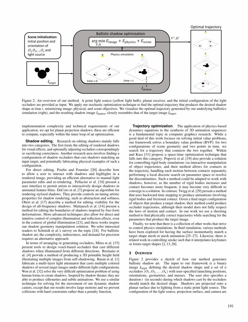
Figure 2: An overview of our method. A point light source (yellow light bulb), planar receiver, and the initial configuration of the lightoccluders are provided as input. We apply our stochastic optimization technique to find the optimal trajectory that produces the desired shadowshape at time t, minimizing image, physical, and scene objectives. We visualize the optimal trajectory generated by our underlying ballisticssimulation (right), and the resulting shadow image Ishadow closely resembles that of the target image Itarget.

implementation complexity and technical requirements of ourapplication, we opt for planar projection shadows; these are efficientto compute, especially within the inner loop of an optimization.

Shadow editing. Research on editing shadows mainly fallsinto two categories. The first treats the editing of rendered shadowsfor visual effects, and optionally adjusting occluders correspondinglyor sacrificing correctness. Another research area involves finding aconfiguration of shadow occluders that cast shadows matching aninput target, and potentially fabricating physical examples of such aconfiguration.

For direct editing, Poulin and Fournier [20] describe howto allow a user to interact with shadows and highlights in arendered image, providing an efficient alternative to manual lightparameter edits and re-rendering. Pellacini et al. [18] present auser interface to permit artists to interactively design shadows inanimated feature films. DeCoro et al. [7] propose an algorithm forrendering stylized shadows. They provide controls on tuning artisticproperties for shadow rendering, such as abstraction and softness.Obert et al. [17] describe a method for editing visibility for thedesign of all-frequency shadows. Mattausch et al. [14] present amethod for editing the boundaries of shadows inspired by free-formdeformations. More advanced techniques also allow for direct andintuitive control of complex illumination and reflection effects, evenin the context of global illumination [23], and these works inspireour shadow geometry manipulation solution. We refer interestedreaders to Schmidt et al.’s survey on the topic [24]. For ballisticshadow art, the complexity, indirectness, and demand for precisionrequires an alternative approach.

In terms of arranging or generating occluders, Mitra et al. [15]present tools to design voxel-based occluders that cast differentshadows when illuminated from different directions. Bermano etal. [4] provide a method of producing a 3D printable height fieldillustrating multiple images from self-shadowing. Baran et al. [1]fabricate a multi-layer light attenuator that casts multiple coloredshadows of several target images under different light configurations.Won et al. [32] solve the very difficult optimization problem of usinghuman forms to create shadows. Inspired by shadow theater, they areable to produce silhouettes and subtle animations. We use a similartechnique for solving for the movement of our dynamic shadowcasters, except that our results involve large motions and we preventcollisions with hard constraints rather than a penalty function.

Trajectory optimization. The application of physics-baseddynamics equations to the synthesis of 3D animation sequencesis a fundamental topic in computer graphics research. While agood deal of this work focuses on solving initial value problems,our framework solves a boundary value problem (BVP): for twoconfigurations of scene geometry and two points in time, wesearch for a trajectory that connects the two together. Witkinand Kass [31] propose a space-time optimization technique thatfalls into this category. Popovic et al. [19] also provide a solutionfor controlling rigid body simulations via interactive manipulationof object trajectories, and their method allows for contacts inthe trajectory, handling each motion between contacts separately,performing a local discrete search on parameter space to resolvethe discontinuities. Such a method could be adapted to work withshadows, however, as the number of rigid bodies increases andcontact becomes more frequent, it may become very difficult toconverge to a solution. In contrast, Twigg et al. [29] present a methodthat uses backward time stepping to produce animations involvingrigid bodies and frictional contact. Given a final target configurationof objects that produce a target shadow, their method could produceoccluder trajectories, although their model does not fully respectthe laws of motion and contact. In our work we use a shootingmethod to find physically correct trajectories while searching for theparameters that produce the target image.

Finally, we note that there is a collection of other works that striveto control physics simulations. In fluid simulation, various methodshave been explored for having the surface momentarily match atarget shape mesh or mesh animation [25–27]. Likewise, there isrelated work in controlling smoke such that it interpolates keyframesor forms target shapes [2, 13, 28].

3 OVERVIEW

Figure 2 provides a sketch of how our method generatesballistic shadow art. The input to our framework is a binaryimage Itarget defining the desired shadow shape and a set of noccluders (O1,O2, . . . ,On) with user-specified launching positions,orientations, geometries, and masses. The user also specifies aduration t (in seconds) during which shadows cast by the occludersshould match the desired shape. Shadows are projected onto aplanar surface due to lighting from a static point light source. Theconfiguration of the light source, projection surface, and camera are

191

part of the scene definition.The core of our framework is a multi-objective optimization that

determines the initial velocities of each occluder such that, at timet, the shadows cast by the occluders closely resemble the targetimage Itarget. Vectors vi ∈ R3 and ωi ∈ R3 store the initial linearand angular velocities, respectively, of each occluder body i, andcollectively for all occluders this is denoted

V = (v1,v2, . . . ,vn) and Ω = (ω1,ω2, . . . ,ωn) .

The optimization finds velocities that minimize a multi-objectivecost function, or formally

argminV, Ω

Eimage +Ephysics +Escene, (1)

where Eimage, Ephysics and Escene are energy functions that introducepenalties pertaining to image, physics, and scene criteria.

We apply a forward dynamics simulation with gravity to updatethe position and orientation of each body. This produces ballistictrajectories that are the signature feature of our framework. Collisiondetection is also enabled, and intersecting bodies generate contactforces to resolve penetration. Since we are optimizing for the initialconditions of a physics simulation involving contacts, the solutionspace is non-convex and highly discontinuous. The CMA-ES [8]method is a stochastic optimization technique that is well-suited tothese conditions, and we use it to minimize Equation 1.

In the next section, we detail the terms that compose each energyfunction and how we compute their values.

4 ENERGY FUNCTIONS

Our energy functions are categorized into three groups: imagecomparison, physics simulation, and scene settings. The imagecomparison functions focus on matching the simulated shadow withthe target image. The physics simulation functions are designedto avoid unreasonable or implausible solutions. Finally, the scenesetting functions penalize unwanted scene arrangements, and alsoprovide an opportunity for users to optionally guide the solution. Forinstance, the user may want a sharp feature of a specific occluder tocorrespond with a particular feature in the target shadow image.

4.1 Image comparisonEnergy functions on image comparison take a simulated shadowimage, Ishadow, and a target shape image, Itarget, as input. Bothimages are represented in binary format, such that

I(x,y) =

1, pixel at (x,y) is in shadow,0, pixel at (x,y) is not in shadow.

The energy function on image space is defined as

Eimage =2

∑i=0

widi +wXOREXOR +winEin +woutEout

where w denotes the weight of the energy term with the correspond-ing subscript, and di is the distance between image moments ofith-order. The simulated shadow and target image are compared withan exclusive-OR operation in EXOR. Finally, Ein and Eout encouragethe inner and outer boundaries of the images to match, respectively.

Image moments distanceImage moments [16] are succinct descriptors of an image andthey are widely used in computer vision and computer graphicsapplications [12, 22]. Because they are effective for carrying low-dimensional information, we include them in our framework.

The energy functions d0, d1, and d2 are the distance between the0th- through to 2nd-order moments of the shadow image, and thetarget shape,

di =∥∥Mi(Ishadow)−Mi(Itarget)

∥∥ ,where Mi is a function computing the ith-order moment of an image.

The 0th-order moment is the total area of the image expressed inpixels. Thus the distance gives the difference of the shadow size.This moment is computed as

M0(I) = ∑x

∑y

I(x,y).

The 1st-order moment represents the 2D centroid of a binaryimage in pixels and the distance is computed by the Euclidean norm.This moment is computed by

M1(I) =(

∑x ∑y x I(x,y) / M0(I)∑x ∑y y I(x,y) / M0(I)

)=

(xy

).

Finally the 2nd-order image moment is a 2×2 matrix[µ20 µ11µ11 µ02

],

whereµpq = ∑

x∑y(x− x)p(y− y)qI(x,y) / M0(I).

This matrix represents the inertia tensor of the input image in twodimensional space. Due to symmetry, the off-diagonal elementsare both µ11. To avoiding repeated calculations in the distance, the2nd-order image moment is defined as a vector

M2(I) =(µ20, µ11, µ02

),

and the distance computed by the Euclidean norm.

Image differenceThe image moments help during early stages of the optimizationby encouraging the shadow to coarsely match the target image. Tosubsequently improve the alignment, we use energy functions thatcompare shadow images at the pixel level. For comparison of thefull image, a binary exclusive-OR operation is performed betweenthe simulated shadow image and the desired shape image:

EXOR = ∑x

∑y

Ishadow(x,y)Y Itarget(x,y).

To improve detail matching, we also design energy functions tomatch the boundaries of the target shape. There are two types ofboundary considered: the inner boundary and the outer boundary.The inner boundary, Ein is defined as

Ein = ∑x

∑y

Ishadow(x,y)∧ Iin(x,y),

with Iin as the inner boundary image. This energy functionencourages the shadow to cover the target silhouette outline byusing the AND operation. For outer boundary matching, we defineEout as

Eout = ∑x

∑y

1− (Ishadow(x,y)∧ Iout(x,y)),

with Iout as the outer boundary image. Similar to the inner boundary,the matching is calculated with a negative-AND operation. With thisdesign, the shadow is discouraged from intersecting the outline.

192

Figure 3: The results obtained with our method for various examples. From left-to-right: Mickey, “fly” Chinese character, “to be continued” inJapanese, and THE THINKER. The target images (top row) are closely matched by the simulated results found by running the optimizationalgorithm (middle row). A comparison of the target and shadow images (bottom row) clearly demonstrates the accuracy. The target images,drawn in black, differ from the simulated shadow images, drawn in red, in only a few small regions.

To compute the boundary images, we apply erosion and dilationoperations to the target image. For the inner and outer boundary,they are computed as

Iin = Itarget− ItargetK,

Iout = Itarget⊕K− Itarget.

We use a simple kernel for image dilation and erosion. We let K bea 5×5 matrix with all elements set to 1.

4.2 Physics simulationThe physics simulation objective guide our optimization towardplausible solutions and avoids unwanted ballistic trajectories. Thereare two terms in this energy function

Ephysics = wcontactEcontact +wregEreg

where Econtact penalizes contact between occluder objects beforetime t, and Ereg serves as a regularization term on the initial linearand angular velocity of shadow casters.

Since contacts are difficult to predict and add noise to the solutionspace, we try to avoid solutions where contact occurs before themoment at which the target shadow shape is formed. The simulationtherefore terminates whenever (i) contact occurs or (ii) the simulationtime reaches t. This ensures a collision free trajectory before time t.

To smoothly guide the optimizer towards a collision free solution,the contact penalty is computed as the difference between the actualsimulation time and the target time t. In other words, it consists

of the time remaining for the simulation to reach the designatedshadow casting moment, and therefore it will be zero if contacts donot occur, or if they only happen at the moment of shadow formation.Formally, this penalty is computed as

Econtact = (t− tsim)ncontact

where tsim is the actual duration of the simulation. The factorncontact is used to scale the time difference by the number of contactsdetected at termination.

We also apply a regularization term, Ereg, to avoid large velocitiesfor the occluders, such that

Ereg = α ∑v∈V‖v‖+(1−α) ∑

ω∈Ω

‖ω‖.

The scalar α ∈ [0,1] is used to balance linear and angular velocitiesin case their magnitudes are significantly different. A value ofα = 0.5 for our examples.

4.3 Scene settingsThe scene setting function ensures that the occluder objectscontribute to the target image in a reasonable way, and we alsotake advantage of human intuition to guide the final configuration ofoccluders. With these objectives in mind, the scene setting energyfunction is defined as

Escene = whintEhint +wbarEbar

193

where Ehint denotes how well the occluders in the scene make useof user defined hints, and Ebar is a barrier function that penalizesoccluders casting shadows out of the desired region.

The energy term for hints is similar to the one used by Wonand Lee [32], which is used to align the projected 3D features of acharacter model to points on the target shadow contour. In our case,we match points on the occluder surface to pixels in the target image.The energy term is defined as

Ehint = ∑h∈H

wh‖P(xh)− ph‖,

where H = h1,h2, . . . ,hk denotes a collection of k hint pointsgiven by the user. Each h is defined as

h = Oi, x, p, w | i ∈ [1,n], x ∈ R3, p ∈ R2, w ∈ R,

and denotes a single hint that matches a location p in image spacewith a position x on occluder Oi; a weighting factor w is used toprioritize hints. The light to plane projection P : R3 7→ R2 is usedto map the 3D coordinate x on the occluder at the time of imageformation to its position in the shadow image. Note that the projectedpoint can be outside the region of the shadow image. The hints usedfor THE THINKER example are shown in Figure 4.

Figure 4: The diagram illustrates how hints are specified as positionson an occluder object, and then mapped to corresponding locationsin the target shadow images (left). All hints used for THE THINKERexample are shown in image space (right).

We design the energy function Ebar to avoid “wasting” occluders.There are cases when one or more occluders do not contribute tothe shadow image because they cast shadows completely outside theimage region. Previous energy functions may fail to prevent this.For instance, if two occluder shadows move outside the region, itis possible that nearby solutions also move the occluders outsideshadow casting region. The energy function could plateau for thesesolutions and convergence will be difficult.

The barrier function is specifically designed to avoid thesesituations and encourage viable solutions. It is defined as

Ebar = ∑i

B(P(Ci)),

with P : R3 7→ R2 the same projection as above, Ci denoting thecenter of mass of occluder i in model space, and B : R2 7→ R thebarrier function on a single occluder:

B(x) =

0, ‖x− c‖< r,‖x− c‖, ‖x− c‖ ≥ r.

Here, c is a point in image space, in this cases we use the centerof the whole image, and r is a user-defined radius. In our case, wechoose half of the image height for the radius.

5 OPTIMIZATION STRATEGIES

As previously noted, the optimization is highly non-linear, duemainly to discontinuities introduced by contacts and the use ofenergy functions computed over binary images. The optimization isalso affected by the “curse of dimensionality” if n is large. For thesereasons, we apply various strategies to guide the optimization andimprove its convergence toward viable solutions. This is especiallyhelpful when there are more than just a few occluders.

We use two main strategies to improve convergence: (i) ascheduled optimization that explores the solution space in stages,and (ii) sequentially solving for trajectories one occluder at a time.We describe these strategies in the following sections.

5.1 Scheduled optimization

Early on in the optimization, the solution space is unexplored.It can therefore be difficult for the optimizer to make progresstowards a viable solution in an error landscape that is wroughtwith local minima. We therefore perform a preliminary stage ofoptimization using only a subset of the energy functions. This tendsto produce a smoother landscape dominated by the image momentand barrier functions, which tend to be less noisy and less proneto high frequency variations. This initial stage helps to guide theparameter sampling and narrow down the solution space.

A subsequent stage of optimization is then seeded using thesolution of the first stage. High frequency energy functions,specifically the XOR comparison, are enabled during this phaseto refine the solution and improve fine scale detail. Figure 6 showsthe solutions at the end of the first and second stages for the Mickeyexample. The energy function weights for this example are alsoprovided in Table 2. Note that the XOR energy is assigned a zeroweight during the first stage, which is then enabled during the secondstage to refine the shadow shape.

During each stage of the optimization, we visualize the best resultof the most recent iteration. The user then stops the current stage andmoves onto the next stage once they are satisfied with the results. Theaccompanying videos demonstrates this visualization. Alternatively,CMA-ES iterations can be stopped once the total energy function issufficiently small, or stagnation occurs and reduction in its value isbelow some small tolerance.

5.2 Sequential optimization of occluders

For complex scenes involving many projectiles, avoiding contactsbetween them becomes difficult if we try to optimize all trajectoriessimultaneously. In particular, when the shadow occluders arelaunched from clustered positions, most of the early solutionsproduce motions that cause the occluders to collide. Even smalldeviations in the parameters result in dramatically different motions.The optimizer converges poorly in such cases since the errorlandscape is noisy.

We improve convergence by optimizing for only one occluderat a time. That is, the initial linear and angular velocity of just asingle occluder is considered during each step of the optimization.Meanwhile, the velocities and trajectories for all other occludersremains fixed. This compromises the automation of our system, butin practice we found that plausible solutions are found much morequickly. This strategy also facilitates backtracking solutions foundfor a specific occluder, since they may be revisited. The order ofoccluders may be automatically generated or defined by the user.This further emphasizes the human-in-the-loop aspect of our system,and provides additional artistic control.

After iterating on all occluders, the user can perform a finalstage of optimization that considers all projectiles at once, but withsmaller sampling deviations.This refines the previous result, and canpotentially help to escape local minima.

194

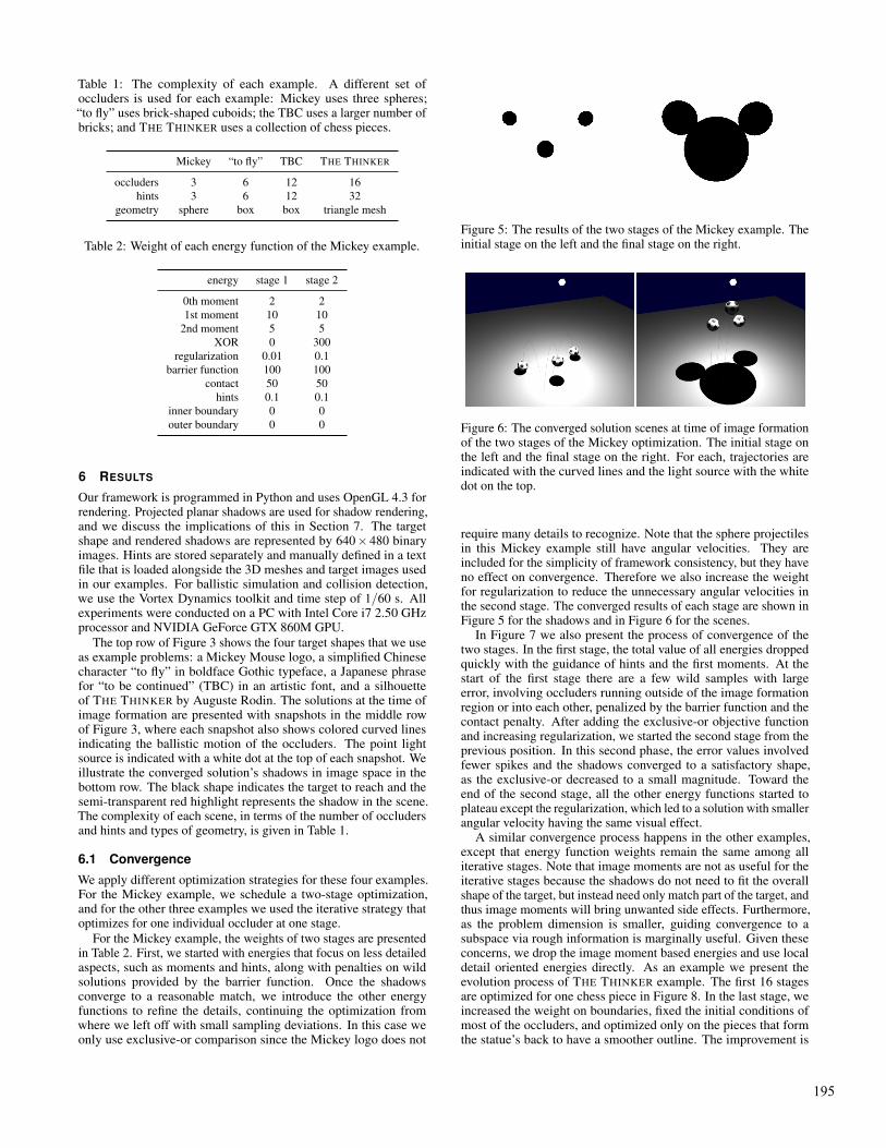
Table 1: The complexity of each example. A different set ofoccluders is used for each example: Mickey uses three spheres;“to fly” uses brick-shaped cuboids; the TBC uses a larger number ofbricks; and THE THINKER uses a collection of chess pieces.

Mickey “to fly” TBC THE THINKER

occluders 3 6 12 16hints 3 6 12 32

geometry sphere box box triangle mesh

Table 2: Weight of each energy function of the Mickey example.

energy stage 1 stage 2

0th moment 2 21st moment 10 10

2nd moment 5 5XOR 0 300

regularization 0.01 0.1barrier function 100 100

contact 50 50hints 0.1 0.1

inner boundary 0 0outer boundary 0 0

6 RESULTS

Our framework is programmed in Python and uses OpenGL 4.3 forrendering. Projected planar shadows are used for shadow rendering,and we discuss the implications of this in Section 7. The targetshape and rendered shadows are represented by 640× 480 binaryimages. Hints are stored separately and manually defined in a textfile that is loaded alongside the 3D meshes and target images usedin our examples. For ballistic simulation and collision detection,we use the Vortex Dynamics toolkit and time step of 1/60 s. Allexperiments were conducted on a PC with Intel Core i7 2.50 GHzprocessor and NVIDIA GeForce GTX 860M GPU.

The top row of Figure 3 shows the four target shapes that we useas example problems: a Mickey Mouse logo, a simplified Chinesecharacter “to fly” in boldface Gothic typeface, a Japanese phrasefor “to be continued” (TBC) in an artistic font, and a silhouetteof THE THINKER by Auguste Rodin. The solutions at the time ofimage formation are presented with snapshots in the middle rowof Figure 3, where each snapshot also shows colored curved linesindicating the ballistic motion of the occluders. The point lightsource is indicated with a white dot at the top of each snapshot. Weillustrate the converged solution’s shadows in image space in thebottom row. The black shape indicates the target to reach and thesemi-transparent red highlight represents the shadow in the scene.The complexity of each scene, in terms of the number of occludersand hints and types of geometry, is given in Table 1.

6.1 Convergence

We apply different optimization strategies for these four examples.For the Mickey example, we schedule a two-stage optimization,and for the other three examples we used the iterative strategy thatoptimizes for one individual occluder at one stage.

For the Mickey example, the weights of two stages are presentedin Table 2. First, we started with energies that focus on less detailedaspects, such as moments and hints, along with penalties on wildsolutions provided by the barrier function. Once the shadowsconverge to a reasonable match, we introduce the other energyfunctions to refine the details, continuing the optimization fromwhere we left off with small sampling deviations. In this case weonly use exclusive-or comparison since the Mickey logo does not

Figure 5: The results of the two stages of the Mickey example. Theinitial stage on the left and the final stage on the right.

Figure 6: The converged solution scenes at time of image formationof the two stages of the Mickey optimization. The initial stage onthe left and the final stage on the right. For each, trajectories areindicated with the curved lines and the light source with the whitedot on the top.

require many details to recognize. Note that the sphere projectilesin this Mickey example still have angular velocities. They areincluded for the simplicity of framework consistency, but they haveno effect on convergence. Therefore we also increase the weightfor regularization to reduce the unnecessary angular velocities inthe second stage. The converged results of each stage are shown inFigure 5 for the shadows and in Figure 6 for the scenes.

In Figure 7 we also present the process of convergence of thetwo stages. In the first stage, the total value of all energies droppedquickly with the guidance of hints and the first moments. At thestart of the first stage there are a few wild samples with largeerror, involving occluders running outside of the image formationregion or into each other, penalized by the barrier function and thecontact penalty. After adding the exclusive-or objective functionand increasing regularization, we started the second stage from theprevious position. In this second phase, the error values involvedfewer spikes and the shadows converged to a satisfactory shape,as the exclusive-or decreased to a small magnitude. Toward theend of the second stage, all the other energy functions started toplateau except the regularization, which led to a solution with smallerangular velocity having the same visual effect.

A similar convergence process happens in the other examples,except that energy function weights remain the same among alliterative stages. Note that image moments are not as useful for theiterative stages because the shadows do not need to fit the overallshape of the target, but instead need only match part of the target, andthus image moments will bring unwanted side effects. Furthermore,as the problem dimension is smaller, guiding convergence to asubspace via rough information is marginally useful. Given theseconcerns, we drop the image moment based energies and use localdetail oriented energies directly. As an example we present theevolution process of THE THINKER example. The first 16 stagesare optimized for one chess piece in Figure 8. In the last stage, weincreased the weight on boundaries, fixed the initial conditions ofmost of the occluders, and optimized only on the pieces that formthe statue’s back to have a smoother outline. The improvement is

195

100

101

102

103

total

100

101

102

103

104

total

10-1

100

101

0th moment

10-510-410-310-210-1100101102

0th moment

10-2

10-1

100

101

1st moment

10-5

10-4

10-3

10-2

10-1

100

101

1st moment

10-1

100

101

2nd moment

10-3

10-2

10-1

100

101

2nd moment

10-1

100

101

102

103

barriercontact

10-1

100

101

102

103

104

barriercontact

10-1

100

101

102

103

hints

10-1

100

101

102

103

hints

10-1

100

reg

100

101

reg

10-1

100

101

102

103

xor

Figure 7: Convergence of the two stages of the Mickey example. The left column presents convergence of the first stage and the right presentsthe second stage. Each figure plots the evaluated value of every sampling instance along the convergence. The red denotes the total of allapplied energies, and the blues denote the weighted value of each energy, short named in the legends. The contact and barrier function areplotted together for space saving purpose. Each plot has a y-axis on log10 scale and therefore the missing values indicate 0. Note the newlyadded exclusive-or function’s plot at the right bottom, and the y-axis with scale may have changed.

196

Figure 8: The evolution of THE THINKER shadows. Each image indicates the converged result of each stage. For every stage there is only onechess piece being manipulated with initial conditions for optimization. The rest of the chess pieces are kept untouched, either remaining still attheir launching positions, casting the small pieces of shadow that line up straight, or adopting the same velocities from last stage convergenceand casting the same shadows.

Figure 9: THE THINKER shadow from the extra stage andcomparisons with the last stage and target. From left to right: thecomparison between the shadow from last stage (blue) and the target(black); the comparison between the shadow of the extra stage (red)and the target (black); the comparison between the shadows of theextra stage (red) and the last stage (blue) where purple indicatesoverlap.

demonstrated in Figure 9. The back of THE THINKER becomessmoother, with a minor trade-off over the stomach. Meanwhile,the rest of THE THINKER is left untouched as the overall shapeis satisfactory given the optimized trajectories of the other chesspieces.

6.2 Performance

In Table 3, we present data indicating how long it takes to convergefor each example. Notice that for more complicated problems, weneed more iterations and samplings to converge. Moreover, usingdifferent optimization strategies makes a difference on convergencetime, as the latter three examples have a low average sampling anditeration number on each stage.

In Table 4, we list the time it takes for computing each energyfunction in milliseconds, except for the energies of regularizationand contacts, which both take less than 0.1 milliseconds. We alsoconducted profiling on ballistic simulations and included thesetimings in the first row of the table. From this we can identify thatone obvious bottle-neck on performance is the physics simulation.Synchronization of threads, the optimization algorithm, hard-driveIO, and other explanations of compute time are not taken intoaccount.

7 DISCUSSION AND FUTURE WORK

The results in Section 6 demonstrate that our framework is capableof synthesizing compelling examples of ballistic shadow art, evenwhen the simulation involves more than a dozen objects and thetarget shadow is complex. The user-in-the-loop aspect of ourframework allows visually pleasing solutions to be found by guidingthe optimization.

Table 3: Performance of optimizations. The optimization processof each example is presented with the numbers of stages, iterations,and samplings. The convergences are also timed and the results aredenoted in minutes and seconds.

Mickey “to fly” TBC THE THINKER

stages 2 6 12 17total iterations 283 458 987 1572

average iterations 141.5 76.3 82.25 98.25total samplings 20376 10992 23688 54048

average samplings 10188.0 1832.0 1974.0 3378.0total running time 29m07s 16m55s 44m57s 396m15s

Table 4: Performance of energy functions. All functions in differentexamples are all timed in milliseconds. For those energy functionsthat are not applied in some examples, the value is labeled as “N/A”;for those not included in this table, the evaluation is trivial and lastsless than 0.1 milliseconds. Besides energy functions, the physicssimulation is also timed and presented.

Mickey “to fly” TBC THE THINKER

simulation 15.2 19.8 31.7 621.00th moment 1.6 N/A N/A N/A1st moment 4.9 N/A N/A N/A

2nd moment 16.1 N/A N/A N/AXOR 8.4 8.3 6.2 7.4

inner boundary N/A N/A N/A 18.7outer boundary N/A N/A N/A 17.2

hints 1.2 1.4 1.4 3.9barrier 1.0 1.6 1.6 2.3

We render shadows by planar projection. Compared to shadowmaps or shadow volumes, projected shadows are easy to implement,efficient to render, and have a perfect resolution, which is usefulfor image comparison purposes. However, this method producesfake shadows when an occluder is located behind the plane, oranti-shadows when it is located behind the light. We note that it ispossible to fix these issues using existing methods [9, 33], but ourtechnique remains limited to shadows cast onto planar receivers. Toexploit the full potential of our framework, we believe it would beinteresting to experiment with shadow mapping or shadow volumes.

There are some factors defining the shadow art problem other thantarget or occluders that we did not enumerate in our experiments. Forinstance, we assume that our shadow art effects are only supposedto be captured from a static camera, which is pointing to thereceiver plane perpendicularly. The light source generally liesabove the shadow center in all cases. To demonstrate the powerof our framework, there should be experiments on problems with

197

more diverse configurations. Scene construction could be furtherautomated by optimizing for the light configuration and cameraparameters. However, this would introduce additional non-linearitiesto the optimization, not to mention increasing the dimensionality ofthe problem.

When comparing the captured and target shadow images, theoptimization attempts to find a perfect match at the target locationthat is specified by the user. An interesting extension for futurework, could investigate translated, rotated or scaled matching. Wecould further improve our framework by accepting slightly deformedshapes [11]. Our framework supports optimizing only a single target,while it is interesting to consider synthesizing shadows for multipletargets. One possibility is to use multiple light sources for thestatic placement of occluders [4, 15] and apply our framework tofind a set of ballistic trajectories. However, this may require verycomplex arrangements of the occluders and thus the convergenceand simulation will be challenging. Another route could be tomatch different target images at different instances along the ballistictrajectory. For example, the projectiles cast a shadow of a targetshape at one instant, and at a later instant they form another targetshadow. Timing becomes critical in such cases, as a poor selection ofinstants by the user may mean there is no feasible physical solution.

Another drawback of our framework is that the resulting effect istransient, and the desired shadow image is formed during only a fewframes of animation. However, we hypothesize that the optimizationcould be coaxed to find solutions where the perceived effect lastsfor a longer duration. For example, by adding an energy functionthat minimizes the spatial velocity of the occluders at time t thiswould implicitly lengthen the duration of the effect. Alternatively,an energy function that explicitly tries to increase the duration of theeffect could also be introduced by evaluating the image differencefunction, EXOR, over a window of frames in the neighborhood of t.

Contacts have been one factor we try to suppress in the framework.The friction and the bounce that contacts produce will lead to atremendous amount of differences in the final status of ballisticmotions, even with minor adjustments to starting conditions.Therefore in the solution space, regions with contacts are filledwith high frequency changes. The sampling on this type of regionis not representative unless small enough deviations are employed.However, because of the dramatic changes that contacts can bring,allowing contacts to occur before matching the target may producemore solutions. For example, we can have two projectiles deflectfrom each other to change their trajectories, so that they can reachplaces in a way that was otherwise impossible. Therefore, this maybe useful for multi-target problems, but it requires the capabilityof optimization algorithms to search within the contact subspaceeffectively.

Finally, successfully fabricating this ballistic shadow art in realitywould be exciting but difficult. To build it we need the physicssimulations to be accurate with respect to air drag and collisionevents. Finally, we would also need to design reliable and accuratemethods for physically launching occluders into desired ballistictrajectories.

ACKNOWLEDGMENTS

The authors gratefully acknowledge the financial support of NSERCand FRQNT.

REFERENCES

[1] I. Baran, P. Keller, D. Bradley, S. Coros, W. Jarosz, D. Nowrouzezahrai,and M. Gross. Manufacturing layered attenuators for multipleprescribed shadow images. Computer Graphics Forum, 2012.

[2] A. Barnat, Z. Li, J. McCann, and N. S. Pollard. Mid-level smokecontrol for 2d animation. In Proc. of Graphics Interface 2011, 2011.

[3] P. Bergeron. A general version of Crow’s shadow volumes. IEEEComputer Graphics and Applications, 1986.

[4] A. Bermano, I. Baran, M. Alexa, and W. Matusk. Shadowpix: Multipleimages from self shadowing. Computer Graphics Forum, 2012.

[5] J. Blinn. Me and my (fake) shadow. IEEE Comput. Graph. andApplications, 1988.

[6] F. C. Crow. Shadow algorithms for computer graphics. SIGGRAPHComput. Graph., 1977.

[7] C. DeCoro, F. Cole, A. Finkelstein, and S. Rusinkiewicz. Stylizedshadows. In Intl. Symp. on Non-Photorealistic Animation andRendering (NPAR). ACM, 2007.

[8] N. Hansen and A. Ostermeier. Adapting arbitrary normal mutationdistributions in evolution strategies: The covariance matrix adaptation.In Proc. of the IEEE Intl. Conf. on Evolutionary Computation, 1996.

[9] P. S. Heckbert and M. Herf. Simulating soft shadows with graphicshardware. Technical report, DTIC Document, 1997.

[10] T. Heidmann. Real shadows, real time. Iris Universe, 1991.[11] T. Igarashi, T. Moscovich, and J. F. Hughes. As-rigid-as-possible shape

manipulation. ACM Trans. on Graph., 2005.[12] J. Lee, J. Chai, P. S. Reitsma, J. K. Hodgins, and N. S. Pollard.

Interactive control of avatars animated with human motion data. ACMTrans. on Graph., 2002.

[13] J. Madill and D. Mould. Target particle control of smoke simulation.In Proc. of Graphics Interface 2013, 2013.

[14] O. Mattausch, T. Igarashi, and M. Wimmer. Freeform shadow boundaryediting. Computer Graphics Forum, 2013.

[15] N. J. Mitra and M. Pauly. Shadow art. ACM Trans. on Graph., 2009.[16] R. Mukundan and K. Ramakrishnan. Moment functions in image

analysis: theory and applications. World Scientific, 1998.[17] J. Obert, F. Pellacini, and S. Pattanaik. Visibility editing for all-

frequency shadow design. Computer Graphics Forum, 2010.[18] F. Pellacini, P. Tole, and D. P. Greenberg. A user interface for interactive

cinematic shadow design. ACM Trans. on Graph., 2002.[19] J. Popovic, S. M. Seitz, M. Erdmann, Z. Popovic, and A. Witkin.

Interactive manipulation of rigid body simulations. In Proc. ofSIGGRAPH 2000, 2000.

[20] P. Poulin and A. Fournier. Lights from highlights and shadows. InProc. of the Symp. on Interactive 3D Graphics, 1992.

[21] W. T. Reeves, D. H. Salesin, and R. L. Cook. Rendering antialiasedshadows with depth maps. SIGGRAPH Comput. Graph., 1987.

[22] L. Ren, G. Shakhnarovich, J. K. Hodgins, H. Pfister, and P. Viola.Learning silhouette features for control of human motion. ACM Trans.on Graph., 2005.

[23] T.-W. Schmidt, J. Novak, J. Meng, A. S. Kaplanyan, T. Reiner,D. Nowrouzezahrai, and C. Dachsbacher. Path-space manipulation ofphysically-based light transport. ACM Trans. on Graph., 2013.

[24] T.-W. Schmidt, F. Pellacini, D. Nowrouzezahrai, W. Jarosz, andC. Dachsbacher. State of the art in artistic editing of appearance,lighting and material. Computer Graphics Forum, 2015.

[25] L. Shi and Y. Yu. Controllable smoke animation with guiding objects.ACM Trans. Graph., 2005.

[26] L. Shi and Y. Yu. Taming liquids for rapidly changing targets. In Proc.of the ACM SIGGRAPH/Eurographics Symp. on Comput. Anim., 2005.

[27] N. Thurey, R. Keiser, M. Pauly, and U. Rude. Detail-preserving fluidcontrol. In Proc. of the ACM SIGGRAPH/Eurographics Symp. onComput. Anim., 2006.

[28] A. Treuille, A. McNamara, Z. Popovic, and J. Stam. Keyframe controlof smoke simulations. ACM Trans. Graph., 2003.

[29] C. D. Twigg and D. L. James. Backward steps in rigid body simulation.ACM Trans. on Graph., 2008.

[30] L. Williams. Casting curved shadows on curved surfaces. SIGGRAPHComput. Graph., 1978.

[31] A. Witkin and M. Kass. Spacetime constraints. SIGGRAPH Comput.Graph., 1988.

[32] J. Won and J. Lee. Shadow theatre: discovering human motion from asequence of silhouettes. ACM Trans. on Graph., 2016.

[33] A. Woo and P. Poulin. Shadow algorithms data miner. CRC Press,2012.

[34] H. Zhang. Forward shadow mapping. In Rendering Techniques.Springer, 1998.

198