An Efficient Parallel Approachfor Identifying Protein Families in Large-scale

Metagenomic Data SetsChangjun Wu, Ananth Kalyanaraman

School of Electrical Engineering and Computer Science

Washington State University

Pullman, WA 99164-2752

Email: cwu2@eecs.wsu.edu, ananth@eecs.wsu.edu

Abstract—Metagenomics is the study of environmental micro-bial communities using state-of-the-art genomic tools. Recentadvancements in high-throughput technologies have enabledthe accumulation of large volumes of metagenomic data thatwas until a couple of years back was deemed impracticalfor generation. A primary bottleneck, however, is in the lackof scalable algorithms and open source software for large-scale data processing. In this paper, we present the designand implementation of a novel parallel approach to identifyprotein families from large-scale metagenomic data. Given aset of peptide sequences we reduce the problem to one of de-tecting arbitrarily-sized dense subgraphs from bipartite graphs.Our approach efficiently parallelizes this task on a distributedmemory machine through a combination of divide-and-conquerand combinatorial pattern matching heuristic techniques. Wepresent performance and quality results of extensively testingour implementation on 160K randomly sampled sequences fromthe CAMERA environmental sequence database using 512 nodesof a BlueGene/L supercomputer.

I. INTRODUCTION

Proteins are fundamental molecules responsible for per-

forming most of the cellular functions in an organism. Proteins

that are evolutionarily- (and thereby functionally-) related are

said to belong to the same “family”. Identifying protein fam-

ilies is of fundamental importance to document the diversity

of the known protein universe. It also provides a means to

determine the functional roles of newly discovered protein

sequences. This latter cause has become highly significant of

late because numerous genome projects have been completed

and as a result there is a sudden expansion of the protein

universe. The most dominant contributor to this information-

revolution has been the projects in metagenomics.

Metagenomics1 [18], the sequencing and analysis of geneticcontent obtained from environmental samples, is a rapidly

emerging area that promises to unravel thousands of pre-

viously unknown microbial species. Among several applica-

tions, metagenomics is expected to create high impact on

bioenergy, environmental biotechnology, pharmaceuticals and

agriculture [17]. In a typical metagenomics project, DNA

1The area has also come to be known as environmental genomics andmicrobial community genomics.

material is collected from a target environment of interest (e.g.,

ocean, acid mine, human gut) and passed through a shotgun

sequencing facility [22]. The collected DNA represents a

pool of microbes living in that environmental sample, and

the shotgun sequencing approach shreds the DNA pool into

millions of tiny “fragments”, each measuring only a few

hundred base pairs (bp). Each of these fragments can then be

individually “sequenced” in a laboratory to have its nucleotide

sequence determined. The resulting environmental sequence

data collection is now ready for computational analysis and

discovery.

Over the last couple of years, numerous metagenomics

projects have been initiated — [13], [25], [30], [31] to name

a few. A continued analysis of their DNA pool is leading to

collections of millions of new amino acid sequences (called

ORFs for Open Reading Frames)2 with a potential to befunctional proteins. The Sorcerer II Global Ocean Sampling

project (henceforth, GOS) [33], which was completed in

March 2007, alone reported over 17 million new ORFs. There

is an immediate need to develop software capable of process-

ing large volumes of ORF sequences along with already known

proteins (also in millions) for an accurate identification of new

protein families or expansion of known families.

There are several accepted ways to define a protein family

[2] — based on protein’s global sequence, domain-level, or

structural similarities. In this paper we consider protein fami-

lies with global and domain similarities. Figure 1 illustrates an

example of a protein domain family. Current approaches for

detecting protein families operate by computing all-versus-all

pairwise sequence similarity, and subsequently using heuristic

techniques to deduce family relationships from pairwise simi-

larities [3], [26], [33]. There are two key limitations to this

approach: (i) Computing all-versus-all pairwise similarities

could become computationally prohibitive even for hundreds

of thousands of sequences because for n sequences the run-

time complexity is Ω(n2). This high complexity is often timesoffset by compromising the quality of the output; and (ii) The

2Henceforth, we use the terms “ORFs” and “amino acid sequences”interchangeably.

Permission to make digital or hard copies of all or part of this work for personal or classroom use is granted without fee provided that copies are not made or distributedfor profit or commercial advantage and that copies bear this notice and the full citation on the first page. To copy otherwise, to republish, to post on servers or to redistribute to lists, requires prior specific permission and/or a fee. SC2008 November 2008, Austin, Texas, USA 978-1-4244-2835-9/08 $25.00 ©2008 IEEE

Fig. 1. A partial alignment of the CRAL/TRIO domain family of proteins, which contains 51 protein members (not all shown). The alignments are fromthe SUPERFAMILY database of structural and functional protein annotations [14].

algorithms to deduce family relationships from pairwise simi-

larities store all pairwise results making the space complexityΘ(n2). While such high complexity in time and space shouldmake the problem an ideal candidate to benefit from parallel

computing, there are hardly any parallel approaches. Even

those that deploy parallelism resort to brute-force allocation of

tasks across multiple computers and to using specialized large-

memory high-end platforms for tackling the space problem.

For example, a recent analysis [33] of ∼28.6 million ORFstook an aggregate 106 CPU hours. The task was parallelized

using 125 dual processors systems and 128 16-processor nodes

each containing between 16GB-64GB of RAM.

In this paper, we present the development of a novel

parallel approach suited to exploit the aggregate memory and

compute power of large scale distributed memory machines

for identifying protein families in large-scale inputs. The key

strengths of our approach are as follows: (i) Using pattern

matching heuristics our approach overcomes the necessity to

compute all-pairs sequence similarities thereby resulting in a

drastic computation reduction in practice; (ii) To overcomethe memory bottleneck, our approach breaks a large problem

instance into numerous small sub-problems, such that each

sub-problem can be solved individually on one compute node.

This divide-and-conquer step is also parallel with an overall

linear memory requirement in the input size; and (iii) Toensure high quality output, our approach reduces the problemto one of finding dense subgraphs in bipartite graphs wherein

there exist several well-studied approximation algorithms. Our

approach is built on ideas from methods developed earlier for

two other applications — genome assembly [19] and dense

subgraph detection for internet data [12].

In what follows, we evaluate existing approaches (Sec-

tion II), outline our approach (Section III), describe our

algorithms (Section IV), and present and discuss the results of

our performance and quality experiments (Section V). Sections

VI and VII summarize the findings and provide new directions

for further research.

II. EXISTING APPROACHES

Several public repositories are available for documenting

proteins along with their family and functional annotation

information [2], [8], [11], [14]–[16], [28]. Protein family

relationships are based on sharing conserved domains [3] or

full-length similarity [26], [33]. Given two sequences, either

of these relationships can be evaluated in time proportional to

the product of sequence lengths using dynamic programming

[23], [27] or even faster using approximate techniques such

as BLAST [1]. Both these techniques account for sequence

mismatches and other differences while trying to maximize

matches.

To the best of our knowledge, the GOS project [33] is

the only work that implements a large-scale methodology for

protein family identification in metagenomic data. Given n

input ORF sequences , the GOS approach can be outlined as

follows:

1) Redundancy removal: Sequences that are more than95% contained in another sequence are deemed re-

dundant and are eliminated from further analysis. This

is accomplished by performing all-versus-all sequence

comparison using the BLASTP program [1].

2) Graph generation: A graph is created with verticesrepresenting the set of non-redundant sequences. An

edge is created between two vertices i and j if and

only if sequences i and j share a “significant” sequence

similarity. The graph is constructed by running the

BLASTP program on all pairs of sequences using a

corresponding similarity cutoff. In their implementation,

the GOS team reports using a 70% similarity cutoff [33].

3) Dense subgraph detection: Because of the expectationthat each sequence in a family is similar to a majority

of its family members, the next step is to analyze the

graph for “dense” subgraphs. However, as a related

optimization problem is NP-Hard [9], the GOS approach

adopts a heuristic strategy of creating sequence core

sets of a bounded size, expanding each core set using

a more relaxed criteria, and merging expanded sets that

intersect.

For parallelization, the set of BLASTP tasks in step (1) are

distributed in parallel to multiple computers. Steps (2) and

(3) require creation of adjacency list and random access and

therefore are implemented using large-memory SMP nodes.

While this approach has been successfully applied to the

..

....

....

....

..

RedundancyRemoval

Connected

DetectionComponentInput

Sequences

NR ...

DenseSubgraphDetection

BipartiteGraph

Generation

Sequences

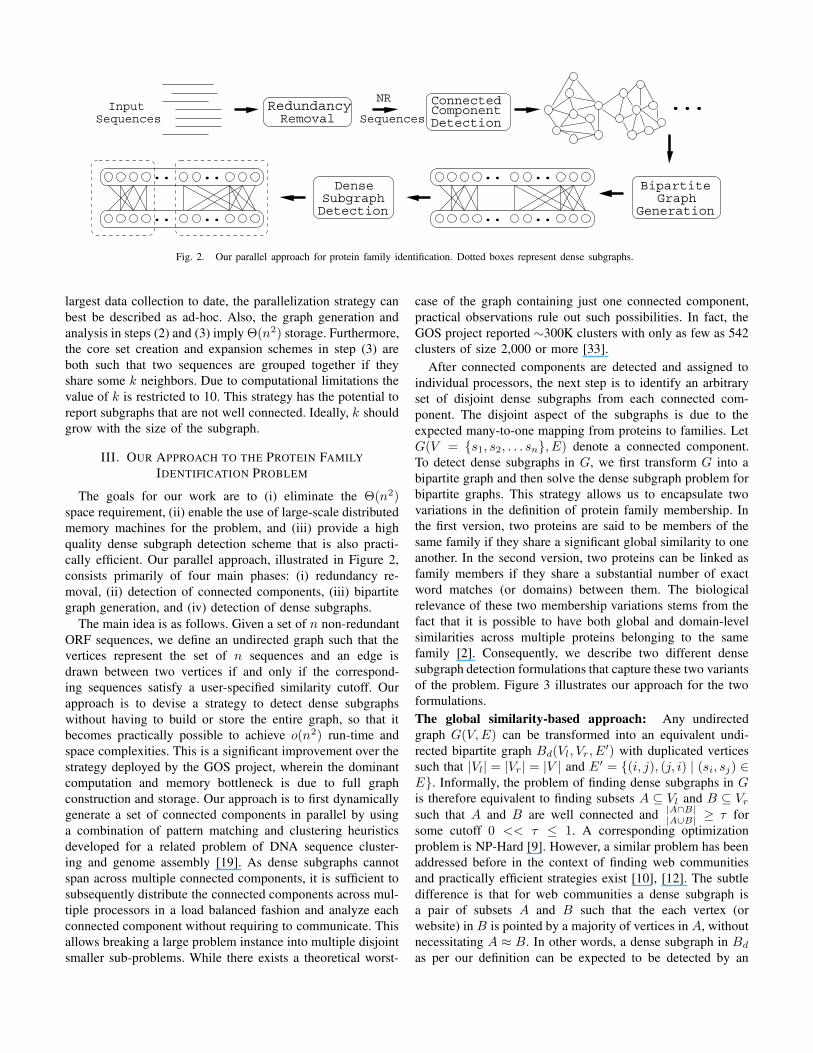
Fig. 2. Our parallel approach for protein family identification. Dotted boxes represent dense subgraphs.

largest data collection to date, the parallelization strategy can

best be described as ad-hoc. Also, the graph generation and

analysis in steps (2) and (3) implyΘ(n2) storage. Furthermore,the core set creation and expansion schemes in step (3) are

both such that two sequences are grouped together if they

share some k neighbors. Due to computational limitations the

value of k is restricted to 10. This strategy has the potential to

report subgraphs that are not well connected. Ideally, k should

grow with the size of the subgraph.

III. OUR APPROACH TO THE PROTEIN FAMILY

IDENTIFICATION PROBLEM

The goals for our work are to (i) eliminate the Θ(n2)space requirement, (ii) enable the use of large-scale distributed

memory machines for the problem, and (iii) provide a high

quality dense subgraph detection scheme that is also practi-

cally efficient. Our parallel approach, illustrated in Figure 2,

consists primarily of four main phases: (i) redundancy re-

moval, (ii) detection of connected components, (iii) bipartite

graph generation, and (iv) detection of dense subgraphs.

The main idea is as follows. Given a set of n non-redundant

ORF sequences, we define an undirected graph such that the

vertices represent the set of n sequences and an edge is

drawn between two vertices if and only if the correspond-

ing sequences satisfy a user-specified similarity cutoff. Our

approach is to devise a strategy to detect dense subgraphs

without having to build or store the entire graph, so that it

becomes practically possible to achieve o(n2) run-time andspace complexities. This is a significant improvement over the

strategy deployed by the GOS project, wherein the dominant

computation and memory bottleneck is due to full graph

construction and storage. Our approach is to first dynamically

generate a set of connected components in parallel by using

a combination of pattern matching and clustering heuristics

developed for a related problem of DNA sequence cluster-

ing and genome assembly [19]. As dense subgraphs cannot

span across multiple connected components, it is sufficient to

subsequently distribute the connected components across mul-

tiple processors in a load balanced fashion and analyze each

connected component without requiring to communicate. This

allows breaking a large problem instance into multiple disjoint

smaller sub-problems. While there exists a theoretical worst-

case of the graph containing just one connected component,

practical observations rule out such possibilities. In fact, the

GOS project reported ∼300K clusters with only as few as 542clusters of size 2,000 or more [33].

After connected components are detected and assigned to

individual processors, the next step is to identify an arbitrary

set of disjoint dense subgraphs from each connected com-

ponent. The disjoint aspect of the subgraphs is due to the

expected many-to-one mapping from proteins to families. Let

G(V = {s1, s2, . . . sn}, E) denote a connected component.To detect dense subgraphs in G, we first transform G into a

bipartite graph and then solve the dense subgraph problem for

bipartite graphs. This strategy allows us to encapsulate two

variations in the definition of protein family membership. In

the first version, two proteins are said to be members of the

same family if they share a significant global similarity to one

another. In the second version, two proteins can be linked as

family members if they share a substantial number of exact

word matches (or domains) between them. The biological

relevance of these two membership variations stems from the

fact that it is possible to have both global and domain-level

similarities across multiple proteins belonging to the same

family [2]. Consequently, we describe two different dense

subgraph detection formulations that capture these two variants

of the problem. Figure 3 illustrates our approach for the two

formulations.

The global similarity-based approach: Any undirected

graph G(V, E) can be transformed into an equivalent undi-rected bipartite graph Bd(Vl, Vr, E

′) with duplicated verticessuch that |Vl| = |Vr | = |V | and E′ = {(i, j), (j, i) | (si, sj) ∈E}. Informally, the problem of finding dense subgraphs in G

is therefore equivalent to finding subsets A ⊆ Vl and B ⊆ Vr

such that A and B are well connected and|A∩B||A∪B| ≥ τ for

some cutoff 0 << τ ≤ 1. A corresponding optimizationproblem is NP-Hard [9]. However, a similar problem has been

addressed before in the context of finding web communities

and practically efficient strategies exist [10], [12]. The subtle

difference is that for web communities a dense subgraph is

a pair of subsets A and B such that the each vertex (or

website) in B is pointed by a majority of vertices in A, without

necessitating A ≈ B. In other words, a dense subgraph in Bd

as per our definition can be expected to be detected by an

..

....

.. ..

....

..

....

....

....

....

GraphSubgraphDetection

DenseSubgraphDetection

Transformation

A

B

Domain−based Graph Reduction

Dense

Global Similarity−based Graph Reduction

TransformationGraph

Connected Component

VmVm

V

V

V

V

V

V

G = (V, E)

Bd :

Bm :

Fig. 3. Illustration of the two dense bipartite subgraph reduction schemes. Dotted boxes represent dense subgraph outputs.

algorithm that solves the corresponding web community dense

subgraph problem. But not every dense subgraph reported by

the latter may satisfy our A ≈ B criterion. But this is an added

constraint that can be tested in a post-processing step. This is

the main idea behind our “global similarity-based” approach.

We use the algorithm by Gibson et al. [12] for generating ourshortlist of dense subgraphs because it is suited for very large

inputs. Henceforth, we refer to this algorithm as the “Shingle”

algorithm.

The domain-based approach: This approach makes a differ-ent bipartite graph reduction which stems from the following

observation: Protein sequences that share multiple domains

can also be expected to share substantially long and possibly

non-contiguous exact matches (as shown in the example in

Figure 1). Therefore, if multiple sequences share a sufficiently

large number of fixed-length exact matches, then they are

likely to belong to the same family. Thus fixed-length exact

matches can be used as supporting evidence to group ORF se-

quences together. To implement this idea, we consider the fol-

lowing bipartite graph construction: Given G = (V, E) as be-fore, let Vm = {e1, e2, . . . em} denote the set of all w−lengthstrings that are present as substrings in at least two different in-

put sequences si and sj , for some fixed w (≈ 10). Let Vr = V .

Then construct a bipartite graph Bm = {Vm, Vr, E′} such that

E′ = {(ei, sj) | ei is a substring in sj}. This constructionmakes the dense subgraph problem equivalent to the web

community version because in the latter’s context websites

are grouped based on the supporting evidence provided by in-

linking websites. Hence, for any pair of subsets A ⊆ Vm and

B ⊆ Vr reported by the Shingle algorithm, our desired dense

subgraph output is B.

IV. ALGORITHMS FOR PARALLEL DETECTION OF PROTEIN

FAMILIES

Let S = {s1, s2, . . . , sn} be the set of n input ORFs; and

� = Σni=1

|si|n. Let p denote the number of processors.

A. Redundancy Removal

Definition 1: Sequence si is said to be “contained” in sj

if an optimal alignment of si with sj satisfies the following

properties: (i) the similarity of the overlapping region is at least

95%; and (ii) at least 95% of si is included in the overlapping

region3.

Problem 1: Given S, remove any si that is contained in any

other sequence.

While this problem can be solved by comparing each pair of

sequences as in the all-versus-all strategy, such an approach

would take Θ(n2�2) run-time. Instead, we apply a standardpattern matching heuristic of designing an exact-match based

filtering technique for shortlisting a set of sequence pairs that

show high promise to exhibit sequence similarity, and later

performing alignment computations [27] only on this reduced

subset. This is achieved by first constructing a generalized

suffix tree (GST) [21] data structure on S and then using it

as a string index for detecting sequence pairs that share a

maximal match of a specified length ψ or greater. To generate

pairs containing maximal matches, we use the optimal parallel

algorithm described in [19]. The value of ψ is determined

by the expected rates of mutation and error tolerance. For

example, if two sequences aligning over a length of 100

characters must contain at least 98% similarity then they

can differ in at most 2 positions, implying that there should

exist at least one matching segment of length 33 characters

or more. Therefore, a 33-character or longer exact match

can be used as a necessary but not sufficient condition for

sequence similarity. The run-time complexity of this phase is

O(n�p

+#pairs generated), and the space complexity is O( n�p

).

The parallel GST construction algorithm runs in O(n�2

p) and

requires O(n�p

) space. Due to lack of space, the algorithmicdetails are omitted. The purpose of redundancy removal is to

eliminate the less trustworthy contained sequences in order to

avoid possible false grouping later during the dense subgraph

stage. Let S′ be the set of non-redundant sequences, and let

|S′| = n′.

3It is to be noted that the cutoffs mentioned as part of our approachthroughout the paper are values that can be specified by the user as soft-ware parameters. The absolute values specified in the paper denote defaultparameter settings.

B. Detection of Connected Components

Definition 2: Two sequences are said to “overlap” if theyshare a local alignment such that the similarity is at least

30% and the alignment includes at least 80% of the longer

sequence.

Problem 2: Given S ′, detect all maximal subsets (or “clus-

ters”) such that each sequence in a cluster overlaps with at

least one other cluster member.

The PaCE parallel algorithm [19] was originally designed

to address this problem although in the context of clustering

DNA sequences. The key steps can be outlined as follows:

1) The algorithm uses the master-worker paradigm.

2) A distributed representation of a GST is generated using

the input S′ on all the worker processors such that each

processor stores a unique O(n′�p

) portion of the tree.3) The master processor initializes the set of clusters such

that each sequence is placed in a cluster of its own.

The clustering is implemented using the union-find data

structure [29] to allow for near-constant time find() andmerge() operations.

4) An iterative process of data exchange between the mas-

ter and workers is started. At each iteration, a worker

processor is responsible for (i) sending new pairs of

sequences that have a significantly long (≥ ψ) maximal

match; these pairs are called promising pairs becausethey have a high likelihood of passing the overlap test,

and (ii) computing alignments [23], [27] over the pairs

of sequences that the master assigned to it. Alternatively,

the master processor is responsible for (i) updating the

current clustering based on the alignment results each

worker returns, (ii) identifying maximal matching pairs

that need alignment computation, and (iii) dynamically

distributing the pending alignment workload to the

worker processors.

Drastic savings in run-time are brought about by heuristic

strategies. At any given time, if two sequences si and sj are

found to have an overlap, then their corresponding clusters are

immediately merged. This is implemented using two find()and one union() operations. This transitive closure mergingscheme is useful because later, if two sequences are reported

as a promising pair and if the master processor locates them

in the same cluster, then there is no necessity to compute

their alignment. To maximize the chance that pairs leading to

cluster merges are found earlier in the process, the dynamic

promising pair detection algorithm generates them directly in

the decreasing order of their maximal match length using an

on-demand scheme as described in [19].

C. Bipartite Graph Generation

For each connected component generated in the previous

phase, a bipartite graph consistent with the reductions de-

scribed in Section III is to be generated. As long as the

connected components are still small enough to fit in the

memory of a single compute node, storing and analyzing a

bipartite graph on a single node is a feasible option. For

example, our implementation can handle a bipartite graph

with up to a total of 16K vertices on a 512 MB RAM, or

equivalently connected components with up to 8K vertices. For

generating these bipartite graphs, however, all pairs of possible

vertices need to be explored for a possible edge, although

the maximal match heuristic can help reduce the work to

some extent. For this reason, we parallelized bipartite graph

generation using a modified version of the PaCE approach in

which we apply only the maximal matching heuristic (and skip

clustering). For the domain-based approach, the algorithm is

much simpler as each fixed-length match identified is to be

connected to their container sequences.

D. Dense Subgraph Detection in Bipartite Graphs

Once bipartite graphs consistent with the preferred

reduction scheme are generated, the next step is to distribute

them to multiple processors and apply the Shingle algorithm

[12] on each bipartite graph serially. We made a few subtle

modifications to the Shingle algorithm to suit the context. To

assess the effectiveness of the algorithm’s application it is

necessary to understand the fundamentals of this algorithm.

Like in the case of the PaCE algorithm, a thorough discussion

is beyond the scope of this paper, and so we focus primarily

on its major steps and the effect of its parameters on our

dense subgraph problem. Most of the following discussions

apply to both the duplicate (Bd) and match-based (Bm)

bipartite approaches.

The Shingle Algorithm: Given a vertex v in an undirected

bipartite graph B = (Vl, Vr, E), Γ(v) denotes the set of itsout-links and is given by {u | (v, u) ∈ E}.

Definition 3: Given parameters (s, c), a “shingle” [7] of avertex v is an arbitrary s−element subset of Γ(v), and an“(s, c)−shingle set” of v is a set of c shingles of v.

Intuitively, two vertices sharing a shingle, by definition,

share s of their out-links. In case of a dense bipartite subgraph,

such pairs of vertices should be plenty on either side. The

Shingle algorithm seeks to group such vertices together and

use them for building dense subgraphs. Larger the value of

s, lesser the probability that two vertices share a shingle, and

vice versa. This implies that a smaller value of s is suited to

enhance the chance of detecting not-so-dense subgraphs. The

parameter c is intended to create the opposite effect. Also,

it is not computationally practical to exhaustively compare

all shingles of each pair of vertices, and the parameter c

offers an alternative to restrict this computation space. This

is achieved by using the min-wise independent permutation

property [6]. Instead of generating c arbitrary shingles for

a vertex v, the algorithm first generates c randomly sorted

permutations of Γ(v) and selects the s minimum elements

from each permutation. Even if two vertices share a modest

number of out-links, the randomness in this property will

ensure that the probability of the vertices sharing a shingle is

sufficiently high. This will be particularly helpful for detecting

large subgraphs, as they are expected to be less dense. These

Report Dense SubgraphPASS I PASS II

B

A

t

s1 ∗ s2s1 ∗ s2Γ(vi)

vjvi

2nd level shingle

1st level shingle

Vl

Vr

Vl

Vr Vr

Vl

S(vi)

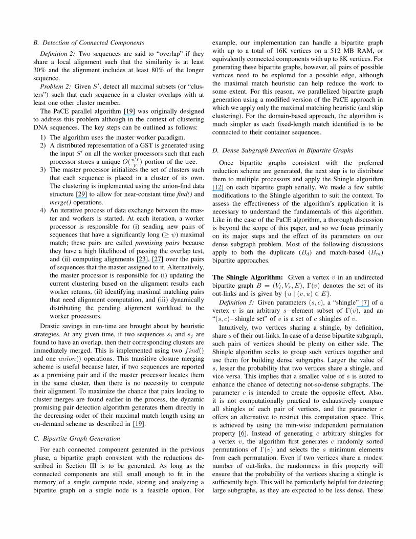
Fig. 4. Illustration of the two-pass Shingle algorithm.

parametric controls make the Shingle algorithm an ideal choice

for our dense subgraph problem.

The algorithm is implemented in two-passes. See Figure 4

for an illustration.

• Pass I: An (s1, c1)-shingle set (denoted by S(vi)) isgenerated for each vertex vi ∈ Vl. For ease of imple-

mentation, each shingle is mapped to an integer using

a hash function. The results are recorded as a 2-tuple

<s(vi), vi>, where s(vi) ∈ S(vi). Let S1 denote the

union of all shingles generated in this pass. Next, vertices

sharing the same shingle are grouped. This is achieved by

sorting the tuples based on shingle values. The resulting

tuple list is input to the second pass.

• Pass II: The algorithm reverses direction and generatesan (s2, c2)-shingle set for each first level shingle s(vi).The result is a set of second level shingles S2, represent-

ing vertices from Vl.

In the final reporting step, all connected components (defined

by S2 shingle to S1 shingle edges) are enumerated and their

constituent vertices recorded. We implemented this using the

union-find data structure. Two subsets of vertices A and B

are reported for each connected component, where A and B

denote the sets of vertices from Vl and Vr respectively. For the

global similarity-based graph approach, we output each A∪B

as one dense subgraph provided it also satisfies the|A∩B||A∪B| ≥ τ

test. For the domain-based approach, we output B directly.

E. Implementation

We implemented our algorithms in C and MPI. The current

version of our implementation only supports global similarity-

based graph approach. To ensure code reuse wherever possible,

we modularized the PaCE software code into separate mod-

ules for generalized suffix tree construction, maximal match

detection, and the master-worker phase for clustering, and

modified them for to work for ORF/amino acid sequences.

The modularized codes were used as the implementation for

the redundancy removal and connected component detection

phases. For bipartite generation we used the maximal match

detection code while implementing a new code for creating

the adjacency list corresponding to each bipartite graph. For

the dense subgraph detection using the Shingle algorithm, we

implemented the code from scratch. Additional scripts were

written to streamline the individual phases into an automated

pipeline.

V. EXPERIMENTAL RESULTS

Our experimental studies were conducted on two platforms:

i) a 512-node BlueGene/L supercomputer with each node

containing two 700 MHz PPC cores and 512 MB RAM; and

ii) a 24-node Linux commodity cluster with a gigabit ethernet

interconnect and each node containing 8 2.33GHz Xeon CPUs

and an 8 GB RAM. All our experiments on the BlueGene/L

were run using the co-processor mode. For the redundancy

removal (RR) and connected component detection (CCD)

phases, we use the BlueGene/L supercomputer. For the dense

subgraph detection (DSD) phase, we used the Linux cluster.

The rationale for using two different platforms is multi-fold.

The BlueGene/L platform enabled us to conduct scalability

studies up to 512 processors; while the Linux cluster provided

a higher per node memory that was required by the DSD code

on connected components with more than 8K vertices. Also,

the 64-bit CPUs in the Linux cluster were more suited for

our implementation of the hash function and random number

generation functionalities.

Data Preparation: The data for our experiments were

downloaded from the CAMERA web portal (http://camera.

calit2.net/), which contains a total of 28.6 million ORFs

spanning different data classes: NCBI-nr [32], PG [32], TGI-

EST [24], ENS [4], [5] and environmental sequences from

the GOS project. The database also hosts the collection of

predicted ORF families (henceforth, referred to as “clusters”)

reported by their team [33]. We extracted two sets of data

from an arbitrary set of clusters such that all sequences

from the selected clusters were used in the analysis. The

first data set contained 160,000 ORFs spanning 221 clusters

with an average sequence length of 163 amino acid residues.

Subsets of this data (10K, 20K, 40K, 80K) were used for

performance evaluation. The second data set contained 22,186

ORFs spanning one large cluster with an average sequence

length of 256 residues.

Qualitative Evaluation: We conducted quality evaluation onthe 22K and 160K data sets. The RR step reduced the two

sets to 21K and 138K respectively. All subsequent analysis

were conducted only on these non-redundant sets. A dense

subgraph minimum size cutoff of 5 was used in our method,

and a fine tuned set of parameters of (5, 300) was usedfor (s, c). The CCD code on the 138K data produced 1.8Kconnected components of size 5 or more. These components

included 95K (out of the 138K) sequences. Each component

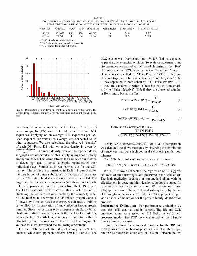
TABLE ITABLE SUMMARY OF OUR QUALITATIVE ASSESSMENT ON THE 22K AND 160K DATA SETS. RESULTS ARE

REPORTED FOR ONLY THOSE CONNECTED COMPONENTS CONTAINING 5 SEQUENCES OR MORE.

#Input seq. #NRaseq. #CCb #DSc #Seq in DS Mean degree Mean density Size of largest DS

160,000 138,633 1,861 850 66,083 26 76% 13,26322,186 21,348 1 134 11,524 20 78% 6,828

a “NR” stands for non-redundant.b “CC” stands for connected components.c “DS” stands for dense subgraphs.

0

10

20

30

40

50

5-910-14

15-1920-24

25-2930-34

40-4445-49

50-5455-59

60-6465-69

70-7475-79

85-8990-94

100-104

120-124

130-134

135-139

165-169

180-184

285-289

Num

ber

of d

ense

sub

grap

hs

Dense subgraph size

Fig. 5. Distribution of our dense subgraphs as a function of their sizes. Thelargest dense subgraph contains over 7K sequences and is not shown in theplot.

was then individually input to the DSD step. Overall, 850

dense subgraphs (DS) were detected, which covered 66K

sequences, implying on an average ∼78 sequences per DS.Each sequence (or vertex) on average was connected to 26

other sequences. We also calculated the observed “density”

of each DS. For a DS with m nodes, density is given by#mean degree

m−1. The mean density over all the reported dense

subgraphs was observed to be 76%, implying high connectivity

among the nodes. This demonstrates the ability of our method

to detect high quality dense subgraphs regardless of their

individual sizes. Similar study was carried out for the 22K

data set. The results are summarized in Table I. Figure 5 shows

the distribution of dense subgraphs as a function of their sizes

for the 22K data. The distribution is skewed as expected. The

largest cluster had over 7K sequences (not shown in the plot).

For comparison we used the results from the GOS project.

The GOS clustering involves several stages. After the initial

clustering (called core set identification), the similarity crite-

ria are relaxed to accommodate far related proteins, and is

followed by a model-based clustering, which uses a training

set to allow for incorporation of knowledge on known protein

families. Since we perform only a sequence similarity based

clustering a direct comparison with the final GOS clustering

cannot be fair. Nevertheless, it is only the sensitivity that is

affected by this discrepancy in the two methodologies. To

validate this, we performed the following assessment.

For the 160K data set, the GOS clustering had 221 final

clusters, while our approach detected 850 DS. For 22K one

GOS cluster was fragmented into 134 DS. This is expected

as per the above sensitivity claim. To evaluate agreements and

discrepancies, we treated our DS-based clustering as the “Test”

clustering and the GOS clustering as the “Benchmark”. A pair

of sequences is called (i) “True Positive” (TP) if they are

clustered together in both schemes; (ii) “True Negative” (TN)

if they separated in both schemes; (iii) “False Positive” (FP)

if they are clustered together in Test but not in Benchmark;

and (iv) “False Negative” (FN) if they are clustered together

in Benchmark but not in Test.

Precision Rate (PR) =TP

TP+FP(1)

Sensitivity (SE) =TP

TP+FN(2)

Overlap Quality (OQ) =TP

TP+FP+FN(3)

Correlation Coefficient (CC) =TP.TN-FP.FN√

(TP+FP).(TN+FN).(TP+FN).(TN+FP)(4)

Ideally, OQ=PR=SE=CC=100%. For a valid comparison,

we calculated the above measures by observing the distribution

of sequences that were included in the clustering under both

schemes.

For 160K the results of comparison are as follows:

PR=95.75%; SE=56.89%; OQ=55.49%; CC=73.04%

While SE is low as expected, the high value of PR suggests

that most of our clustering is also preserved in the Benchmark.

The high prediction accuracy of our method along with its

effectiveness in detecting high density subgraphs is suited for

generating a more accurate core set. We believe our dense

subgraph detection scheme followed subsequently by the set

of thorough evaluations performed in the GOS project can pro-

vide an ideal combination for the protein family identification

problem.

Performance Evaluation: For performance evaluation we

used the 160K data set and its subsets. The RR and CCD

implementations were tested on 512 BG/L nodes (in co-

processor mode). The DSD code was tested on the 24-node

Linux commodity cluster.

Figure 6a shows the combined run-time for the RR and

CCD phases as a function of processor size. The 160K input

run on 512 processors completed in 3h 20m. Between the two

0

4000

8000

12000

16000

20000

24000

4 5 6 7 8 9 10

Run

-tim

e (s

ec)

lg(Number of processors)

n=10kn=20kn=40k n=80k

n=160k

0

4000

8000

12000

16000

20000

24000

0 20 40 60 80 100 120 140 160

Run

-tim

e (s

ec)

Number of sequences (in thousands)

p=32p=64

p=128 p=512

(a) (b)

Fig. 6. Parallel run-times (in seconds) on BG/L for the RR and CCD phases as a function of (a) processor size, and (b) input size.

0

2

4

6

8

10

12

14

16

18

20

4 5 6 7 8 9 10

Spe

edup

lg(Number of processors)

n=10kn=20kn=40kn=80k

ideal

0

400

800

1200

1600

2000

2400

2800

0 20 40 60 80

Run

-tim

e (s

ec)

Number of sequences (in thousands)

S=5, C=100S=5, C=200S=5, C=300S=5, C=400

(a) (b)

Fig. 7. (a) Speedup of the RR and CCD phases for varying input sizes on 512 nodes of a BlueGene/L supercomputer. The minimum processor size usedwas 32 nodes, and hence the speedup figures are calculated relative to a 32-node system. Also, due to a technical (resource management) restriction it wasnot possible to launch jobs on a 256 node system. (b) Serial run-time for dense subgraph detection as a function of input size and (s, c) parameter values.

phases, the RR phase accounted for more than 90% of all

run-times. This is as expected because detection of redundant

sequences do not lead to any clustering. The CCD phase is

faster when compared to the RR phase because successfully

tested alignments lead to merging of clusters, and thereby

result in drastic reductions in alignment work. For example,

on the 40K input 168 million promising pairs were generated

based on maximal matches of length 10 residues, and of which

only 7 million pairs were selected for alignment computations.

This corresponds to a 99% in work reduction when compared

to any scheme that deploys an all-versus-approach approach

((40K

2

) ≈ 800 million alignment computations). Figure 6bshows run-times as a function of the input size. While the

run-time has an asymptotic worst-case quadratic complexity,

the efficacy of the clustering heuristic technique varies with

the input data.

Figure 7a shows the speedup of executing the RR and CCD

phases. As can be observed, the speedup figures are closer

to linear for larger input sizes; while for higher number of

processors (e.g., 128 to 512) there is only a modest increase

in speedup (e.g., from 3.6 to 6.7 vs. an ideal 4 to 16). Upon

investigation, we found that this loss in expected speedup was

due to the CCD phase. As a concrete example, consider the

80K input case, for which the respective run-times for the

RR and CCD are tabulated in Table II. As can be noted, the

scaling of the RR phase, which is the most dominant phase, is

mostly linear; whereas, there is poor scaling of the CCD phase.

During the CCD phase, the clustering heuristic eliminates an

overwhelming majority (more than 99.9%) of the promising

pairs generated based on maximal matches. As a result, the

work generated by the worker processors were being too

aggressively filtered out on the master node, thereby leaving

very little alignment work to be redistributed to the worker

nodes. This is both a beneficial and undesirable outcome

— beneficial because only an insignificant fraction of the

overall pairs generated are actually aligned thereby drastically

reducing the overall time to solution; and undesirable because

the work reduction adversely affects the scaling. A more

aggressive work generation scheme is required to compensate

for work loss.

TABLE IIRUN-TIMES (IN SECONDS) FOR THE RR AND CCD PHASES FOR THE 80K

INPUT CASE.

PhaseNumber of processors

32 64 128 512

RR 17,476 10,296 4,560 2,207CCD 1,068 777 528 670

The dense subgraph detection phase was relatively faster

when compared to the previous phases. Even on the largest

connected component recorded in our experiments (∼20K),the serial code took less than 10 minutes on a single processor

of the linux cluster. The average run-time for connected

components generated for the 160K input was ∼3 minutes.Because of the short run-times for each connected component,

we grouped multiple connected components into batches of

roughly the same size and distributed the batches across

processors. The plot in Figure 7b shows the run-time statistics

on these groupings as a function of input size and shingle

parameters, s and c. It can be observed that the run-time

increases with increasing values of the c parameter. This is

because more shingles will be generated and hence increase

the overall workload.

VI. FUTURE WORK

We plan to continue the development effort in several

directions.

• Quality testing: The effect of similarity cutoffs and otherparameters on the quality of the protein family prediction

is to be studied. More extensive qualitative validations

are necessary to ascertain the merits of our approach for

large-scale identification of protein families in metage-

nomic data sets. In addition, we plan to implement, test

and compare the domain-based family detection approach

proposed in this paper.

• Parallelization of the Shingle algorithm: While timeis not likely to be an issue for the dense subgraph

detection phase (at least for the range of inputs tested),

our goal is to parallelize the shingle step to address the

need for memory. Currently, if all shingles on either side

of the bipartite graph are unique then the peak space

requirement is proportional to O(m×c2), where m is the

cardinality of the smaller of the partitions in the bipartite

graph.

• Large-scale application: While our experiments on

small to medium-sized inputs show promising perfor-

mance and quality results, tens of millions of new se-

quence data are becoming rapidly available. Perhaps a

greater challenge will be to extend the methodologies

developed here to solve problems of much larger scales

with improved quality.

VII. CONCLUSIONS

We presented a novel parallel approach for protein fam-

ily identification. This is a challenging problem of growing

significance, and is an ideal application to benefit from super-

computing technologies. We draw from the strengths of two

methods (PaCE and Shingle) previously developed for other

applications, and apply them in context of a new problem.

Overall the results presented in this paper demonstrate the high

potential and positive impact of parallelism for metagenomic

protein family identification. They have also pointed us to

many new research directions for further investigation.

ACKNOWLEDGMENTS

We would like to thank Prof. Srinivas Aluru at Iowa State

University for granting access to BlueGene/L. We also wish to

thank the anonymous reviewers for their detailed and insightful

comments on a preliminary version of this manuscript. This

research was supported in parts by the Washington State

University Foundation and the Office of Research.

REFERENCES

[1] S.F. Altschul, W. Gish, W. Miller et al. Basic local alignment search tool.Journal of Molecular Biology, 215:403–410, 1990.

[2] R. Apweiler, A. Bairoch and C.H. Wu. Protein sequence databases.Current Opinion in Chemical Biology, 8(1):76–80, 2004.

[3] A. Bateman, L. Coin, R. Durbin et al. The Pfam protein families database.Nucleic Acids Research, 32:D138–141, 2004.

[4] E. Birney, T.D. Andrews, P. Bevan et al. An overview of Ensembl.Genome Research, 14(5):925–928, 2004.

[5] E. Birney, T.D. Andrews, P. Bevan et al. Ensembl 2004.. Nucleic AcidsResearch, 32(Database issue):D468–470, 2004.

[6] A.Z. Broder, M. Charikar, A. Frieze and M. Mitzenmacher. Min-wiseindependent permutations. Journal of Computer and System Sciences,60:630–659, 2000.

[7] A.Z. Broder, S. Glassman, M. Manasse and G. Zweig. Syntactic clusteringof the web. WWW6/Computer Networks, 29:1157–1166, 1997.

[8] F. Corpet, J. Gouzy and D. Kahn. The ProDom database of proteindomain families. Nucleic Acids Research, 26(1):323–326, 1998.

[9] U. Feige, D. Peleg and G. Kortsarz. The dense k-subgraph problem.Algorithmica, 29(3):410–421, 2001.

[10] G.W. Flake, S. Lawrence and C.L. Giles. Efficient identification of webcommunities. In Proc. ACM SIGKDD, pages 150–160, 2000.

[11] E. Gasteiger , E. Jung and A. Bairoch SWISS-PROT: connectingbiomolecular knowledge via a protein database. Current Issues inMolecular Biology, 3(3):47–55, 2001.

[12] D. Gibson, R. Kumar and A. Tomkins. Discovering large densesubgraphs in massive graphs. In Proc. VLDB Conference, pages 721–732, 2005.

[13] S.R. Gill, M. Pop, R.T. DeBoy et al. Metagenomic analysis of thehuman distal gut microbiome. Science, 312(5778):1355–1359, 2006.

[14] J. Gough, K. Karplus, R. Hughey and C. Chothia. Assignment ofhomology to genome sequences using a library of Hidden Markov Modelsthat represent all proteins of known structure. Journal of MolecularBiology, 313(4):903–919, 2001.

[15] D.H. Haft, B.J. Loftus, D.L. Richardson et al. TIGRFAMs: a proteinfamily resource for the functional identification of proteins. Nucleic AcidsResearch, 29(1):41–3, 2001.

[16] D.H. Haft, J.D. Selengut and O. White. The TIGRFAMs database ofprotein families. Nucleic Acids Research, 31(1):371–373, 2003.

[17] J. Handelsman. Metagenomics: Application of genomics to uncul-tured microorganisms. Microbiology and Molecular Biology Reviews,68(4):669–685, 2004.

[18] J. Handelsman, M.R. Rondon, S.F. Brady et al. Molecular biologicalaccess to the chemistry of unknown soil microbes: a new frontier fornatural products. Chemistry & Biololgy, 5:R245–R249, 1998.

[19] A. Kalyanaraman, S.J. Emrich, P.S. Schnable and S. Aluru. Assemblinggenomes on large-scale parallel computers. Journal of Parallel andDistributed Computing, 67:1240–1255, 2007.

[20] R. Kumar, P. Raghavan, S. Rajagopalan and A. Tomkins. Extractinglarge scale knowledge bases from the web. In Proc. VLDB Conference,pages 639–650, 1999.

[21] E. McCreight. A space economical suffix tree construction algorithm.Journal of the ACM, 23:262–272, 1976.

[22] E.W. Myers, G.G. Sutton, A.L. Delcher et al. A Whole-GenomeAssembly of Drosophila. Science, 287:2196–2204, 2000.

[23] S.B. Needleman and C.D. Wunsch. A general method applicable tothe search for similarities in the amino acid sequence of two proteins.Journal of Molecular Biology, 48:443–453, 1970.

[24] J. Quackenbush, F. Liang, I. Holt et al. The TIGR gene indices:reconstruction and representation of expressed gene sequences.. NucleicAcids Research, 28(1):141–145, 2000.

[25] D.B. Rusch, A.L. Halpern, G. Sutton et al. The Sorcerer II GlobalOcean Sampling Expedition: Northwest Atlantic through Eastern TropicalPacific. PLoS Biology, 5(3):e77, 2007.

[26] O. Sasson, A. Vaaknin, H. Fleischer et al. ProtoNet: hierarchicalclassification of the protein space. Nucleic Acids Research, 31(1):348–352, 2003.

[27] T.F. Smith and M.S. Waterman. Identification of common molecularsubsequences. Journal of Molecular Biology, 147:195–197, 1981.

[28] E.L. Sonnhammer, S.R. Eddy, E. Birney et al. Pfam: multiple sequencealignments and HMM-profiles of protein domains. Nucleic Acids Re-search, 26(1):320–322, 1998.

[29] R.E. Tarjan. Efficiency of a good but not linear set union algorithm.Journal of the ACM, 22(2):215–225, 1975.

[30] S.G. Tringe, C. Mering, A. Kobayashi et al. Comparative metagenomicsof microbial communities. Science, 308(5721):554–557, 2005.

[31] J.C. Venter, K. Remington, J.F. Heidelberg et al. Environmental genomeshotgun sequencing of the Sargasso Sea. Science, 304(5667):66–74, 2004.

[32] D.L. Wheeler, C. Chappey, A.E. Lash et al. Database resources of theNational Center for Biotechnology Information. Nucleic Acids Research,28(1):10–14, 2000.

[33] S. Yooseph, G. Sutton, D. B. Rusch et al. The Sorcerer II Global OceanSampling Expedition: Expanding the Universe of Protein Families. PLoSBiology, 5(3):e16, 2007.