The Language of Julia Donaldson: Rhetoric, Style and Cognition
arX
iv:m
ath/
0610
340v
2 [
mat
h.D
S] 2
9 Se
p 20
07
COMPUTABILITY OF JULIA SETS
MARK BRAVERMAN, MICHAEL YAMPOLSKY
Abstract. In this paper we settle most of the open questions on algorithmic computabil-ity of Julia sets. In particular, we present an algorithm for constructing quadratics whoseJulia sets are uncomputable. We also show that a filled Julia set of a polynomial is alwayscomputable.
Contents
1. Foreword 12. Introduction to computability 23. Julia sets of rational mappings 114. Preliminary results on computability of Julia sets 235. Positive results 266. Computability of Julia sets of Siegel quadratics and negative results 307. Interpretation of the results 36Appendix A. Proof of Proposition 3.18 43Appendix B. Proof of Lemmas 6.8, 6.9 and 6.10 44References 48
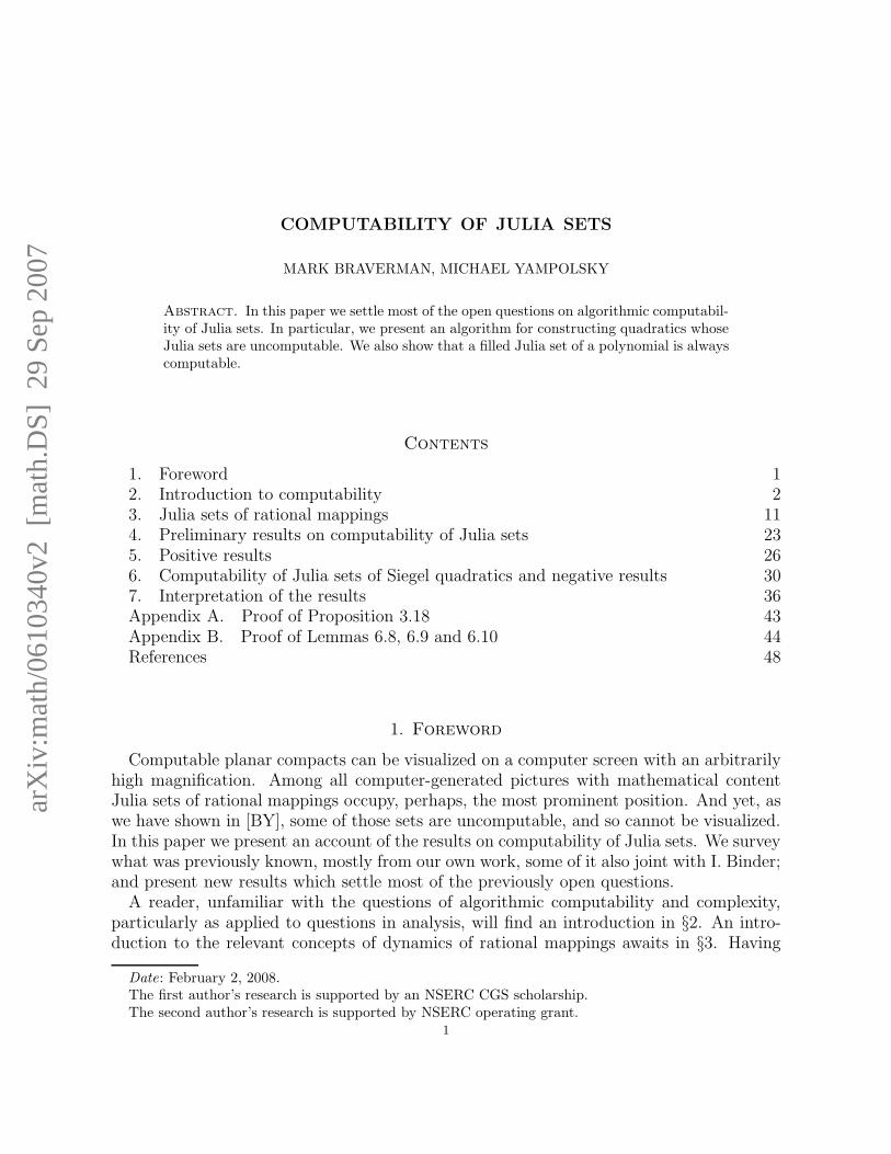
1. Foreword
Computable planar compacts can be visualized on a computer screen with an arbitrarilyhigh magnification. Among all computer-generated pictures with mathematical contentJulia sets of rational mappings occupy, perhaps, the most prominent position. And yet, aswe have shown in [BY], some of those sets are uncomputable, and so cannot be visualized.In this paper we present an account of the results on computability of Julia sets. We surveywhat was previously known, mostly from our own work, some of it also joint with I. Binder;and present new results which settle most of the previously open questions.
A reader, unfamiliar with the questions of algorithmic computability and complexity,particularly as applied to questions in analysis, will find an introduction in §2. An intro-duction to the relevant concepts of dynamics of rational mappings awaits in §3. Having
Date: February 2, 2008.The first author’s research is supported by an NSERC CGS scholarship.The second author’s research is supported by NSERC operating grant.
1

2 MARK BRAVERMAN, MICHAEL YAMPOLSKY
thus set the stage, we derive some preliminary results on computability of Julia sets in §4.In §5 we present our first new result:
All filled Julia sets of polynomial mappings are algorithmically computable.
This answers in the positive a question put to us by John Milnor. In the following §6 wediscuss negative results. In particular, we show:
There exist computable complex parameters c, such that the Julia set of J(z2 + c) is notalgorithmically computable.
Previously, we could only show the existence of parameters for which the Julia set isuncomputable. Now we can give an algorithm for their construction. The question whethersuch a thing is possible would be invariably asked by our colleagues after our talks on thesubject. The general feeling was, perhaps, that the uncomputability of Julia sets is in someways connected to lack of computability of c’s. As we see now, this is not the case.
In the final §7 we interpret our results, and attempt to describe a toy model for uncom-putable Julia sets. We also try to answer the “naıve” question: “What would a computerreally draw, when J(z2 + c) is uncomputable?” Much of the discussion in this section ismotivated by a problem posed to us by Michael Shub.
We now have a good understanding of computable properties of rational Julia sets. Inthis paper, however, we completely avoid discussing the related computational complexityquestions. In this area we know comparatively little. In [BBY2], jointly with I. Binder,we have shown that computational complexity of quadratic Julia sets can be arbitrarilyhigh. Evidently, there is an interplay between dynamical properties of Julia sets, and thehardness of drawing their picture on a computer screen. However, as the work [Brv3] of thefirst author suggests, this connection may not be straightforward: it shows that a class ofmaps with “bad” dynamical properties has poly-time computable Julia sets. Undoubtedly,many similar surprises still await us in this line of investigation.
Acknowledgements. It is our pleasure to thank our friend and colleague Ilia Binderfor the many useful discussions on computability of Julia sets. We thank John Milnorfor posing the question on computability of filled Julia sets to us. We are grateful toMichael Shub for formulating a question which has motivated much of the discussion on the“shape” of uncomputable Julia sets in this paper. We also wish to thank many colleagueswho have invariably asked us if parameters for uncomputable Julia sets can be producedalgorithmically.
2. Introduction to computability
One of the main goals of computability theory is to classify problems according towhether or not they can be solved algorithmically. In fact, such questions existed beforecomputers. A famous example is Hilbert’s Tenth Problem:
“Given a diophantine equation with any number of unknown quantities and with rationalintegral numerical coefficients: to devise a process according to which it can be determined

COMPUTABILITY OF JULIA SETS 3
by a finite number of operations whether the equation is solvable in rational integers.”[Bulletin of the American Mathematical Society 8 (1902), 437-479.]
In other words:
Is it algorithmically possible to determine if a given diophantine equation is solvable?
It is fairly clear what an affirmative answer would mean in this case – a method to checkif an equation has a solution. Giving a negative answer (which turns out to be the correctone) requires a more formal definition of “methods” that can be used in the solution – asone would need to prove that none of these methods work. A universaly accepted modelwas introduced in 1936 in a seminal work by Turing [Tur] in the form of a Turing Machine.
2.1. Discrete computability and the Turing Machine. The definition of a TuringMachine (TM) is somewhat technical and can be found in all texts on computability eg.[Pap, Sip]. The computational power of a Turing Machine is equivalent to that of a RAMcomputer, and one can think of it as a program on such a computer. The program can use afinite amount of memory at each stage of the computation, but it can always request more,and there is no a-priori limit on the amount of memory that the machine uses. In fact,there is a general belief, usually referred to as the Church-Turing thesis, which states thatany computation performed on a physical device can be simulated using a Turing Machine.Just as an ordinary computer program, any Turing Machine admits a finite description.
The definition of a Turing Machines gives a natural way of classifying the computabilityof functions in the discrete setting, such as functions acting on the set of naturals N or theset of finite binary strings 0, 1∗. Namely, a function f(x) is computable, if there exists aTM which takes x as an input and outputs the value f(x).
Computable functions are sometimes called recursive. They include simple functionssuch as integer arithmetic operations and lexicographical sorting of strings. They alsoinclude problems that appear to be difficult in practice, but can be solved nonethelessif we are willing to wait sufficiently long. These include, for example, finding the primefactorization of an integer and finding the optimal strategy in the game of Go.
On the other hand, there are many functions that are not computable. One argument tosee this is a simple counting argument: any TM has a finite description, and hence thereare countably many TMs. On the other hand, there are uncountably many functions fromN to N, or even from N to 0, 1 – and thus “most” functions are not computable. It ismuch more iteresting to have specific examples of non-computability.
One such example is the Halting Problem. The halting function H maps a pair (T, w)where T is an encoding of a TM M and w is a binary input to 1 if the machine M runningon input w eventually halts, and 0 otherwise.
Sketch of proof that H is not computable. The proof is by a simple diagonalization argu-ment. Suppose there were a TM M1 computing the halting function. Let M2 be thefollowing machine: on an input w, M2 uses M1 to compute H(w,w). If H(w,w) = 0, thenM2 halts, otherwise it goes into an infinite loop.

4 MARK BRAVERMAN, MICHAEL YAMPOLSKY
Let w2 be the encoding of M2. What will be the outcome of running M2(w2)? If M2
halts on w2, then H(w2, w2) = 1, and thus M2 cannot halt on w2 by definition. If M2 failsto halt on w2, then H(w2, w2) = 0, and by its definition M2 halts on input w2. In eithercase we arrive at a contradiction.
Consider a predicate A : N×N→ 0, 1 defined as follows. On an input (x, t), A viewesx as an encoding of a pair (M,w) of a TM and an input. A(x, t) is 1 if and only if x gives avalid encoding and M halts on w in exactly t steps. It is easy to see that A is a computablepredicate using a simple simulation. On the other hand, computing the predicate
B(x) = ∃t A(x, t)
is as difficult as solving the Halting Problem, and thus B is non-computable. This examplewill be useful later on. More generally, a predicate of the form P (x) = ∃y R(x, y) for acomputable predicate R(x, y) is said to be recursively enumerable. Moreover, R(x, y) canbe modified, so that for every x there exists at most one y such that R(x, y) holds. Weemphasize this by writing P (x) = ∃!y R(x, y) Note that any recursive predicate is alsorecursively enumerable.
Another explicit example of a non-conputable function is given by the negative solutionto Hilbert’s Tenth Problem, which is due to Matiyasevich (see [Mat] for details and thehistory of the problem).
Theorem 2.1. The function that maps an encoding of a diophantine equation E to 1 if Eis solvable and to 0 otherwise, is non-compuable.
One of Turing’s original motivations for introducing the Turing Machine was classifyingreal numbers into computable and non-computable ones. A number is said to be com-putable if there exists a TM that writes its (infinite) decimal expansion digit by digit. Anequivalent, but slightly less representation dependent is the following definition.
Definition 2.1. A real number α is said to be computable, if there is a computable function
φ : N→ N such that for all n,∣∣∣α− φ(n)
2n
∣∣∣ < 2−n. The set of the computable reals is denoted
by RC.
In other words, there exists an algorithm to approximate α with any desired degree ofprecision. As with discrete functions, “most” numbers are non-computable, while most“nice” numbers such as π and e are. It can be shown that RC with the usual arithmeticoperations forms a closed real field.
Here we give an extension of the computable numbers that will be useful later on in thepaper.
Definition 2.2. A real number α is said to be right computable, if there is a computablefunction φ : N→ Q such that
• the sequence φ(n) is nonincreasing: φ(1) ≥ φ(2) ≥ . . .; and• the sequence φ(n) converges to α: limn→∞ φ(n) = α.

COMPUTABILITY OF JULIA SETS 5
It is obvious that a computable real number is also right-computable. The converse isnot true in general:
Proposition 2.2. Right computable numbers form a dense subset in R \ RC.
Proof. It is obviously sufficient to present a single right computable number which is notcomputable, as then a dense set can be produced using simple arithmetic manipulations.Let P (x) = ∃!y R(x, y) be a non-computable predicate on N such that R(x, y) is com-putable, as discussed above. Consider the number
α = 1−∞∑
x=1
P (x) · 4−x.
Then α is non-computable, since computing α would also enable us to compute the pred-icate P . On the other hand, α is right computable, as demonstrated by the followingcomputable function:
φ(n) = 1−n∑
x=1
n∑
y=1
R(x, y) · 4−x.
φ(n) is obviously non-increasing, and
limn→∞
φ(n) = 1−∞∑
x=1
∞∑
y=1
R(x, y) · 4−x = 1−∞∑
x=1
P (x) · 4−x = α.
A more detailed discussion on the different extensions of the concept of a computablenumber can be found in [Wei].
The above definition of computability using Turing Machines directly applies only tocomputability questions for discrete objects. It has to be extended if we want to discusscomputability of continuous objects such as functions over R or subsets of Rk.
2.2. Oracle computation, computable real functions. The history of defining com-putability for real objects probably begins with the work of Banach and Mazur [BM] of1937, only one year after Turing’s paper. This work has founded the tradition of Com-putable Analysis (sometimes also called Constructive Analysis). Interrupted by war, itwas further developed in the book by Mazur [Maz]. Much research took place in the mid1950’s in the works of Grzegorczyk [Grz], Lacombe [Lac], and others. A parallel schoolof Constructive Analysis was founded by A. A. Markov in Russia in the late 1940’s. Amodern treatment of the field can be found in [Ko1] and [Wei].
The definition of computability over the reals presented here falls into this framework.Consider the simplest case in which we would like to compute a function f : R→ R. On
an input x, we are trying to compute f(x). As in the case with real numbers, the machineM computing f should be able to output f(x) with any given precision 2−n. The machineM , as well as a practical computer, can only handle a finite amount of information, andthus is not capable of reading or storing an entire input x. Instead, it is allowed to request
6 MARK BRAVERMAN, MICHAEL YAMPOLSKY
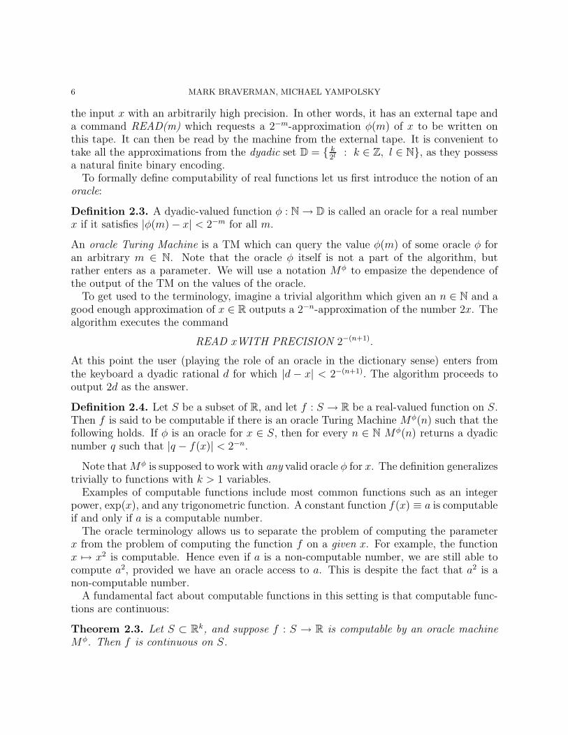
the input x with an arbitrarily high precision. In other words, it has an external tape anda command READ(m) which requests a 2−m-approximation φ(m) of x to be written onthis tape. It can then be read by the machine from the external tape. It is convenient totake all the approximations from the dyadic set D = k
2l : k ∈ Z, l ∈ N, as they possessa natural finite binary encoding.
To formally define computability of real functions let us first introduce the notion of anoracle:
Definition 2.3. A dyadic-valued function φ : N→ D is called an oracle for a real numberx if it satisfies |φ(m)− x| < 2−m for all m.
An oracle Turing Machine is a TM which can query the value φ(m) of some oracle φ foran arbitrary m ∈ N. Note that the oracle φ itself is not a part of the algorithm, butrather enters as a parameter. We will use a notation Mφ to empasize the dependence ofthe output of the TM on the values of the oracle.
To get used to the terminology, imagine a trivial algorithm which given an n ∈ N and agood enough approximation of x ∈ R outputs a 2−n-approximation of the number 2x. Thealgorithm executes the command
READ xWITH PRECISION 2−(n+1).
At this point the user (playing the role of an oracle in the dictionary sense) enters fromthe keyboard a dyadic rational d for which |d − x| < 2−(n+1). The algorithm proceeds tooutput 2d as the answer.
Definition 2.4. Let S be a subset of R, and let f : S → R be a real-valued function on S.Then f is said to be computable if there is an oracle Turing Machine Mφ(n) such that thefollowing holds. If φ is an oracle for x ∈ S, then for every n ∈ N Mφ(n) returns a dyadicnumber q such that |q − f(x)| < 2−n.
Note thatMφ is supposed to work with any valid oracle φ for x. The definition generalizestrivially to functions with k > 1 variables.
Examples of computable functions include most common functions such as an integerpower, exp(x), and any trigonometric function. A constant function f(x) ≡ a is computableif and only if a is a computable number.
The oracle terminology allows us to separate the problem of computing the parameterx from the problem of computing the function f on a given x. For example, the functionx 7→ x2 is computable. Hence even if a is a non-computable number, we are still able tocompute a2, provided we have an oracle access to a. This is despite the fact that a2 is anon-computable number.
A fundamental fact about computable functions in this setting is that computable func-tions are continuous:
Theorem 2.3. Let S ⊂ Rk, and suppose f : S → R is computable by an oracle machineMφ. Then f is continuous on S.

COMPUTABILITY OF JULIA SETS 7
Proof. Let x ∈ S and ε > 0 be given. Choose an integer m such that 2−m < ε/2. Letφ(n) be an oracle for x such that |φ(n) − x| < 2−(n+1) for all n (thus “exceeding” theminimum requirement from an oracle). Then Mφ(m) otputs a number d ∈ D such that|d − f(x)| < 2−m. It terminates after finitely many steps, and hence φ is only queriedup to some finite precision 2−k. It is now not hard to see that for any x′ such that|x− x′| < 2−k−1, there is a valid oracle φ′ which agrees with φ up to precision 2−k. Thusfor any x′ ∈ S ∩ (x− 2−k−1, x+ 2−k−1), Mφ′
(m) outputs the same answer d, and we musthave |d− f(x′)| < 2−m. Hence for every x′ ∈ S such that |x− x′| < 2−k−1, we have
|f(x)− f(x′)| ≤ |f(x)− d|+ |f(x′)− d| < 2−m + 2−m < ε.
In particular, it shows that discontinuous functions, such as arcsin or χQ cannot be com-puted by a single machine on the whole domain of definition.Same considerations can be used to prove a stronger result:
Theorem 2.4. In the conditions of Theorem 2.3 there exists a computable function µ(x, k) :S ×N→ N such that
|f(y)− f(x)| < 2−k whenever y ∈ S and |y − x| < 2−µ(x,k).
We will refer to the this property by saying that f has a computable local modulus ofcontinuity.
Remark 2.1. In some cases, for example when S = [0, 1], the global modulus of continuity(or simply the modulus of continuity) of f on S is also computable. That is, we cancompute a function µ : N→ N such that
(2.1) for any x, y ∈ S with |x− y| < 2−µ(k) ⇒ |f(x)− f(y)| < 2−k.
More generally, this is true whenever S is a compact computable set (as will be defined inthe next section). In particular, this is true whenever S = [a, b] with computable endpointsa and b, or when S is the unit circle in R2.
2.3. Computability of subsets of Rk. Let K ⊂ Rk be a compact set. We would liketo give a definition for K being computable. In the discrete case the distinction betweencomputability of functions and sets is not as important, since a set S is usually said to becomputable, or decidable, if and only if its characteristic function χS is computable. Thesame definition would not work over R, since only continuous functions can be computable,hence χK would not be computable unless K = ∅.
We say that a TM M computes the set K if it approximates K in the Hausdorff metric.Recall that the Hausdorff metric is a metric on compact subsets of Rk defined by
dH(X, Y ) = infǫ > 0|X ⊂ Uǫ(Y ) and Y ⊂ Uǫ(X).We approximate K using a class C of sets which is dense in metric dH among compact sets,and such that elements of C have a natural binary encoding. Namely C is the set of finite

8 MARK BRAVERMAN, MICHAEL YAMPOLSKY
unions of dyadic balls:
C =
n⋃
i=1
B(di, ri) | where di ∈ Dk, ri ∈ D
.
Members of C can be encoded as binary strings in a natural way. The following definitionis equivalent to the set computability definition given in [Wei], and in earlier works (e.g.[RW]).
Definition 2.5. We say that a compact set K ⊂ Rk is computable, if exists a TM M(m),such that on input m, M(m) outputs an encoding of Cm ∈ C such that dH(K,Cm) < 2−m.
To illustrate the robustness of this definition we present the following two equivalentcharacterizations of computable sets (see e.g. [Brv]). The first one relates the definitionto computer graphics. It is made more precise in the discussion below. The second onerelates the computability of sets to the computability of functions as per Definition 2.4.
Theorem 2.5. For a compact K ⊂ Rk the following are equivalent:(1) K is computable as per definition 2.5,(2) (in the case k = 2) K can be drawn on a computer screen with arbitrarily high
resolution,(3) the distance function dK(x) = inf|x − y| | y ∈ K is computable as per definition
2.4.
Let us elaborate further on part (2) of the theorem. A “drawing” P of the set K on thecomputer screen is just a collection of pixels that serve as an accurate description of K (ora portion of K, if the image is zoomed-in). We would expect the following properties fromP :
• P should include all pixels that intersect with K, this guarantees that we get apicture of the entire set P ; and• P should not include pixels that are “far” from K, for example pixels that are at
least one pixel diameter away from the set K.
By switching from the rectangular computer pixels to the mathematically more convenientround pixels, we see that to “draw” K one should be able to compute a function fK :D×Dk → 0, 1 from the family
(2.2) fK(d, r) =
1 if B(d, r) ∩K 6= ∅0 if B(d, 2 · r) ∩K = ∅0 or 1 otherwise
fK then can be used to decide whether to include a round pixel with center d and radiusr in P . Sample values of the function fK are illustrated on Figure 1.
2.4. Weakly computable sets. In this section we present a different definition of set-computability, we call weak computability. If was first introduced by Chou and Ko [CK].

COMPUTABILITY OF JULIA SETS 9
Figure 1. Sample values of the function fK
Definition 2.6. We say that a set S is weakly computable if there is an oracle TuringMachine Mφ(n) such that if φ = (φ1, φ2, . . . , φk) represents a point x = (x1, . . . , xk) ∈ Rk,then the output of Mφ(n) is
(2.3) Mφ(n) =
1 if x ∈ K0 if B(x, 2−(n−1)) ∩K = ∅0 or 1 otherwise
Condition (2.3) is similar to condition (2.2). The difference is that now we allow x to beany point in Rk (not just Dk), and we do not require the machine to output 1 if x is notin K but is “close”. It is evident from Figure 2 that Definition 2.6 requires less effort fromthe algorithm computing K than the original definition. Thus, the new definition appearsto be weaker than the defintion of set computability from last section, but it turns out thatthey are equivalent.
Theorem 2.6. [Brv2] A compact set K ⊂ Rk is weakly computable if and only if it iscomputable as per definition 2.5.
It is sometimes easier to use weak computability when proving that a certain set iscomputable. We will use Theorem 2.6 in §7.
2.5. Set-valued functions and uniformity. The problem of computing Julia sets isessentially that of mapping the coefficients of a rational function R(z) to the set JR. Thuswe need a notion of computability of set-valued functions to discuss computability questionsabout Julia sets.
We can now combine the definitions from previous sections to define computability ofset valued functions.
Definition 2.7. Let S be a subset of Rk. Denote by K∗ℓ the set of all the compact subsets
of Rℓ. Let F : S → K∗ℓ be a set-valued function mapping points in S to compact subsets of

10 MARK BRAVERMAN, MICHAEL YAMPOLSKY
Figure 2. The values of fK(•, 2−n) in the definitions of regular (left) andweak set computability
Rℓ. F is said to be computable on S if there is an oracle TM Mφ1,...,φk(n) that for oraclesrepresenting a point x = (x1, x2, . . . , xk) ∈ S outputs an encoding of a set Cn ∈ C suchthat the Hausdorff distance dH(F (x), Cn) < 2−n.
In fact, the computability definitions for real functions, sets, and set-valued functionspresented above fit in nicely within the much more general framework of Type Two Effi-ciency (TTE). See [Wei], and references therein for more details. In particular, Theorem2.3 stating that computable ⇒ continuous holds in a very broad variety of settings. Wewill only need it in the case of set-valued functions. The proof is very similar to the proofof Theorem 2.3 (see e.g. [BY]).
Theorem 2.7. Suppose F : S ⊂ Rk → K∗ℓ is computable as per Definition 2.7, then F is
continous on S in the Hausdorff metric.
Example. Let the complex plane C be naturally identified with R2. Let d > 1 be aninteger. Consider the multi-valued function fd = d
√: C → C. There is no continuous
single-valued branch of fd on the entire complex plane, hence there is no computable branchif fd that is defined on the entire C. There is a computable branch of fd that is definedeverywhere except for a slit connecting 0 to ∞.
On the other hand, if we view the function fd as a set-valued function that maps anumber z = r · e2πiθ to its d roots r1/d · e2πiθ/d, r1/d · e2πi(θ+1)/d, . . . , r1/d · e2πi(θ+d−1)/d, thenit is not hard to see that fd becomes computable. And indeed, the map fd : R2 → K∗
2 iscontinuous in the Hausdorff metric.

COMPUTABILITY OF JULIA SETS 11
Note that Definition 2.7 makes sense even when S = s is a singleton. In this casewe say that F is nonuniformly computable on s. Otherwise, we say that F is uniformlycomputable on the set S.
Remark on the BSS computability model. We note that another approach to com-putability of subsets of Rk has been developed by Blum, Shub, and Smale [BCSS]. It isbased on the concept of decidability in the Blum-Shub-Smale (BSS) model of real com-putation. The BSS model is very different from the Computable Analysis model we use,and can be very roughly described as based on computation with infinite-precision realarithmetic. Some discussion of the differences between the models may be found in [BrC]and [Brv2]. Algebraic in nature, BSS decidability is not well-suited for the study of fractalobjects, such as Julia sets. It turns out (see Chapter 2.4 of [BCSS]) that in the BSS modelall, but the most trivial Julia sets are not decidable. More generally, sets with a fractionalHausdorff dimension, including ones with very simple description, such as the Cantor set,are BSS-undecidable.
3. Julia sets of rational mappings
3.1. Basic properties of Julia sets. An excellent general reference for the material inthis section is the book of Milnor [Mil]. For a rational mapping R of degree degR = d ≥ 2considered as a dynamical system on the Riemann sphere
R : C→ C
the Julia set is defined as the complement of the set where the dynamics is Lyapunov-stable:
Definition 3.1. Denote F (R) the set of points z ∈ C having an open neighborhood U(z)on which the family of iterates Rn|U(z) is equicontinuous. The set F (R) is called the Fatou
set of R and its complement J(R) = C \ F (R) is the Julia set.
In the case when the rational mapping is a polynomial
P (z) = a0 + a1z + · · ·+ adzd : C→ C
an equivalent way of defining the Julia set is as follows. Obviously, there exists a neigh-borhood of ∞ on C on which the iterates of P uniformly converge to ∞. Denoting A(∞)the maximal such domain of attraction of ∞ we have A(∞) ⊂ F (R). We then have
J(P ) = ∂A(∞).
The bounded set C \ A(∞) is called the filled Julia set, and denoted K(P ); it consists ofpoints whose orbits under P remain bounded:
K(P ) = z ∈ C| supn|P n(z)| <∞.
For future reference, let us summarize in a proposition below the main properties of Juliasets:

12 MARK BRAVERMAN, MICHAEL YAMPOLSKY
Proposition 3.1. Let R : C → C be a rational function. Then the following propertieshold:
• J(R) is a non-empty compact subset of C which is completely invariant: R−1(J(R)) =J(R);• J(R) = J(Rn) for all n ∈ N;• J(R) has no isolated points;
• if J(R) has non-empty interior, then it is the whole of C;
• let U ⊂ C be any open set with U ∩ J(R) 6= ∅. Then there exists n ∈ N such thatRn(U) ⊃ J(R);• periodic orbits of R are dense in J(R).
Let us further comment on the last property. For a periodic point z0 = Rp(z0) of periodp its multiplier is the quantity λ = λ(z0) = DRp(z0). We may speak of the multiplier of aperiodic cycle, as it is the same for all points in the cycle by the Chain Rule. In the casewhen |λ| 6= 1, the dynamics in a sufficiently small neighborhood of the cycle is governed bythe Mean Value Theorem: when |λ| < 1, the cycle is attracting (super-attracting if λ = 0),if |λ| > 1 it is repelling. Both in the attracting and repelling cases, the dynamics can belocally linearized:
(3.1) ψ(Rp(z)) = λ · ψ(z)
where ψ is a conformal mapping of a small neighborhood of z0 to a disk around 0.In the case when |λ| = 1, so that λ = e2πiθ, θ ∈ R, the simplest to study is the paraboliccase when θ = n/m ∈ Q, so λ is a root of unity. In this case Rp is not locally linearizable; itis not hard to see that z0 ∈ J(R). The description of the dynamics in a small neighborhoodof a parabolic orbit will be discussed below in some detail.
In the complementary situation, two non-vacuous possibilities are considered: Cremercase, when Rp is not linearizable, and Siegel case, when it is. In the latter case, thelinearizing map ψ from (3.1) conjugates the dynamics of Rp on a neighborhood U(z0) tothe irrational rotation by angle θ (the rotation angle) on a disk around the origin. Themaximal such neighborhood of z0 is called a Siegel disk.
A different kind of a rotation domain may occur only for a non-polynomial rationalmapping R. A Herman ring A is a conformal image
ν : z ∈ C| 0 < r < |z| < 1 → A,
such that
Rp ν(z) = ν(e2πiθz),
for some p ∈ N and θ ∈ R \Q.The term basin in what follows will describe the set of points whose orbits converge to agiven periodic orbit under the iteration of R. We will denote Postcrit(R) the post-criticalset of R, defined as the closure of the union of the orbits of critical points of R. Fatoumade the following observation:

COMPUTABILITY OF JULIA SETS 13
Proposition 3.2. Let p1, . . . , pk be a periodic orbit of a rational mapping R. If it is eitherattracting, or parabolic, then its basin contains a critical point of R.
By a perturbative argument, Fatou then concluded that for a rational mapping R withdegR = d ≥ 2 at most finitely many periodic orbits are non-repelling. A sharp bound ontheir number depending on d has been established by Shishikura; it is equal to the numberof critical points of R counted with multiplicity:
Fatou-Shishikura Bound. For a rational mapping of degree d the number of the non-repelling periodic cycles taken together with the number of cycles of Herman rings is atmost 2d− 2. For a polynomial of degree d the number of non-repelling periodic cycles in C
is at most d− 1.
Therefore, we may refine the last statement of Proposition 3.1:
• repelling periodic orbits are dense in J(R).
Classical results of Fatou also imply the following:
Proposition 3.3. Every Cremer point of a rational mapping R as well as every point ofthe boundary of a Siegel disk or a Herman ring is contained in Postcrit(R).
By definition, the basin of an attracting or a parabolic point, as well as preimagesof Siegel disks and Herman rings belong to the Fatou set. Fatou-Sullivan ClassificationTheorem formulated below rules out other possibilities:
Fatou-Sullivan Classification. For every connected component W ⊂ FR there existsm ∈ N such that the image H = Rm(W ) is periodic under the dynamics of R. Moreover,each periodic Fatou component H is of one of the following types:
• a component of the basin of an attracting or a super-attracting periodic orbit;• a component of the basin of a parabolic periodic orbit;• a Siegel disk;• a Herman ring.
To conclude the discussion of the basic properties of Julia sets, let us consider the sim-plest examples of non-linear rational endomorphisms of the Riemann sphere, the quadraticpolynomials. Every affine conjugacy class of quadratic polynomials has a unique represen-tative of the form fc(z) = z2 + c, the family
fc(z) = z2 + c, c ∈ C
is often referred to as the quadratic family. For a quadratic map the structure of the Juliaset is governed by the behavior of the orbit of the only finite critical point 0. In particular,the following dichotomy holds:
Proposition 3.4. Let K = K(fc) denote the filled Julia set of fc, and J = J(fc) = ∂K.Then:
• 0 ∈ K implies that K is a connected, compact subset of the plane with connectedcomplement;
14 MARK BRAVERMAN, MICHAEL YAMPOLSKY
• 0 /∈ K implies that K = J is a planar Cantor set.
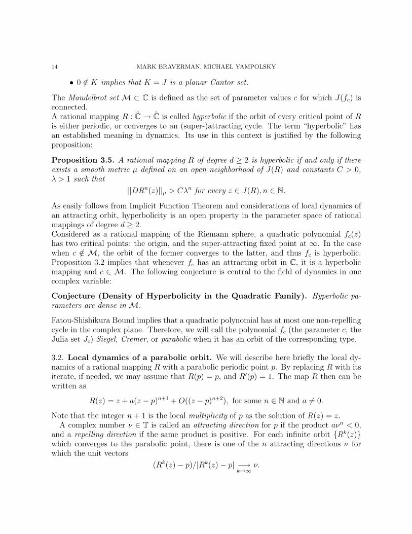
The Mandelbrot set M ⊂ C is defined as the set of parameter values c for which J(fc) isconnected.A rational mapping R : C→ C is called hyperbolic if the orbit of every critical point of Ris either periodic, or converges to an (super-)attracting cycle. The term “hyperbolic” hasan established meaning in dynamics. Its use in this context is justified by the followingproposition:
Proposition 3.5. A rational mapping R of degree d ≥ 2 is hyperbolic if and only if thereexists a smooth metric µ defined on an open neighborhood of J(R) and constants C > 0,λ > 1 such that
||DRn(z)||µ > Cλn for every z ∈ J(R), n ∈ N.
As easily follows from Implicit Function Theorem and considerations of local dynamics ofan attracting orbit, hyperbolicity is an open property in the parameter space of rationalmappings of degree d ≥ 2.Considered as a rational mapping of the Riemann sphere, a quadratic polynomial fc(z)has two critical points: the origin, and the super-attracting fixed point at ∞. In the casewhen c /∈ M, the orbit of the former converges to the latter, and thus fc is hyperbolic.Proposition 3.2 implies that whenever fc has an attracting orbit in C, it is a hyperbolicmapping and c ∈ M. The following conjecture is central to the field of dynamics in onecomplex variable:
Conjecture (Density of Hyperbolicity in the Quadratic Family). Hyperbolic pa-rameters are dense in M.
Fatou-Shishikura Bound implies that a quadratic polynomial has at most one non-repellingcycle in the complex plane. Therefore, we will call the polynomial fc (the parameter c, theJulia set Jc) Siegel, Cremer, or parabolic when it has an orbit of the corresponding type.
3.2. Local dynamics of a parabolic orbit. We will describe here briefly the local dy-namics of a rational mapping R with a parabolic periodic point p. By replacing R with itsiterate, if needed, we may assume that R(p) = p, and R′(p) = 1. The map R then can bewritten as
R(z) = z + a(z − p)n+1 +O((z − p)n+2), for some n ∈ N and a 6= 0.
Note that the integer n + 1 is the local multiplicity of p as the solution of R(z) = z.A complex number ν ∈ T is called an attracting direction for p if the product aνn < 0,
and a repelling direction if the same product is positive. For each infinite orbit Rk(z)which converges to the parabolic point, there is one of the n attracting directions ν forwhich the unit vectors
(Rk(z)− p)/|Rk(z)− p| −→k→∞
ν.

COMPUTABILITY OF JULIA SETS 15
We say in this case that the orbit converges to p in the direction of ν. For each attractingdirection ν, we say that a topological disk U is an attracting petal of R at p if the followingproperties hold:
• U ∋ p;• Rn(U) ⊂ U ∪ p;• an infinite orbit Rk(z) is eventually contained in U if and only if it converges top in the direction of ν.
Similarly, U is a repelling petal for R if it is an attracting petal for the local branch of R−1
which fixes p.
Figure 3. A Leau-Fatou flower with three attracting petals (shaded) andthree repelling petals (emphasized). The attracting and repelling directionsare also indicated. The arrows show the direction of the orbits in one of thepetals; the image of this petal is also indicated.
The petals form a Leau-Fatou Flower at p:
Theorem 3.6. There exists a collection of n attracting petals P ai , and n repelling petals P r
j
such that the following holds. Any two repelling petals do not intersect, and every repellingpetal intersects exactly two attracting petals. Similar properties hold for attracting petals.The union
(∪P ai ) ∪ (∪P r
j ) ∪ pforms an open simply-connected nighborhood of p.
The proof of this statement is based on a multivalued change of coordinates
w = κ(z) =c
(z − p)n, where c = − 1
na.

16 MARK BRAVERMAN, MICHAEL YAMPOLSKY
The map κ conformally transforms the infinite sector between two repelling directions intothe plane with the negative real axis removed. In this sector, it changes the map R into
F (w) = w + 1 +O(1/ n√|w|), as w →∞.
Selecting a right half-plane Hr = Re z > r for a sufficiently large r > 0, we have
ReF (w) > Rew + 1/2, and hence F (H) ⊂ H.
The corresponding attracting petal can then be chosen as the domain κ−1(H), using theappropriate branch of the inverse. Note, that given the coefficients of the rational mappingR, the description of the petal is constructive. Let us formulate this last statement in alanguage suitable for later references:
Lemma 3.7. For each degree d ≥ 2 there exists an oracle Turing Machine Mφ such thatthe following holds. Let R be a rational mapping of degree d with a parabolic periodic pointp, with period m and multiplier e2πis/t. Let n be the number of attracting (and repelling)directions at p. The machine Mφ takes as input the values of m, n, s, t and a naturalnumber k; it is given oracle access to the coefficients of R and the value of p. It outputs aset Lk ∈ C such that the following is true:
• Lk+1 ⊃ Lk and ∪ Lk = P is the union of attracting petals of R at p, covering allthe attracting directions;• distH(Lk, P ) < 2−k.
The dynamics inside a petal is described by the following:
Proposition 3.8. Let P be an attracting or repelling petal of R. Then the quotient man-ifold P/z∼R(z) is conformally isomorphic to the cylinder C/Z.
In other words, in each of the petals there exists a conformal change of coordinates trans-forming R(z) into the unit translation z 7→ z + 1.
Suppose now that the multiplier of the fixed point p is a q-th root of unity, R′(p) = e2πip/q,where (p, q) = 1. A fixed petal for the iterate Rq corresponds to a cycle of q petals for R.It thus follows that q divides the number n of attracting/repelling directions of p as a fixedpoint of Rq. We make note of the following proposition, due to Fatou:
Proposition 3.9. Each cycle of attracting petals of a rational mapping R captures an orbitof a critical point of R.
This implies, in particular, that a quadratic polynomial fc with a parabolic periodic pointζ with multiplier e2πip/q has a Leau-Fatou flower at ζ with a single cycle of q attractingpetals.
3.3. Occurence of Siegel disks and Cremer points in the quadratic family. Let usdiscuss in more detail the occurrence of Siegel disks in the quadratic family. For a number

COMPUTABILITY OF JULIA SETS 17
θ ∈ [0, 1) denote [r1, r2, . . . , rn, . . .], ri ∈ N ∪ ∞ its possibly finite continued fractionexpansion:
(3.2) [r1, r2, . . . , rn, . . .] ≡1
r1 +1
r2 +1
· · ·+ 1
rn + · · ·Such an expansion is defined uniquely if and only if θ /∈ Q. In this case, the rationalconvergents pn/qn = [r1, . . . , rn] are the closest rational approximants of θ among thenumbers with denominators not exceeding qn. In fact, setting λ = e2πiθ, we have
|λh − 1| > |λqn − 1| for all 0 < h < qn+1, h 6= qn.
The difference |λqn − 1| lies between 2/qn+1 and 2π/qn+1, therefore the rate of growth ofthe denominators qn describes how well θ may be approximated with rationals.
Definition 3.2. The diophantine numbers of order k, denoted D(k) is the following classof irrationals “badly” approximated by rationals. By definition, θ ∈ D(k) if there existsc > 0 such that
qn+1 < cqk−1n
The numbers qn can be calculated from the recurrent relation
qn+1 = rn+1qn + qn−1, with q0 = 0, q1 = 1.
Therefore, θ ∈ D(2) if and only if the sequence ri is bounded. Dynamicists call suchnumbers bounded type (number-theorists prefer constant type). An extreme example of anumber of bounded type is the golden mean
θ∗ =
√5− 1
2= [1, 1, 1, . . .].
The set
D(2+) ≡⋂
k>2
Dk
has full measure in the interval [0, 1). In 1942 Siegel showed:
Theorem 3.10 ([Sie]). Let R be an analytic map with a periodic point z0 ∈ C of period p.Suppose the multiplier of the cycle
λ = e2πiθ with θ ∈ D(2+),
then the local linearization equation (3.1) holds.
The strongest known generalization of this result was proved by Brjuno in 1972:

18 MARK BRAVERMAN, MICHAEL YAMPOLSKY
Theorem 3.11 ([Bru]). Suppose
(3.3) B(θ) =∑
n
log(qn+1)
qn<∞,
then the conclusion of Siegel’s Theorem holds.
Figure 4. The Julia set of Pθ for θ = [1, 1, 1, 1, . . .] (the inverse golden mean).
Note that a quadratic polynomial with a fixed Sigel disk with rotation angle θ after anaffine change of coordinates can be written as
(3.4) Pθ(z) = z2 + e2πiθz.
In 1987 Yoccoz [Yoc] proved the following converse to Brjuno’s Theorem:
Theorem 3.12 ([Yoc]). Suppose that for θ ∈ [0, 1) the polynomial Pθ has a Siegel point atthe origin. Then B(θ) <∞.
The numbers satisfying (3.3) are called Brjuno numbers; the set of all Brjuno numbers willbe denoted B. It is evident that ∪D(k) ⊂ B and thus the set B has full measure in theunit circle. On the other hand, it can be shown that its complement is dense-Gδ.
The sum of the series (3.3) is called the Brjuno function. For us a different character-ization of B will be more useful. Inductively define θ1 = θ and θn+1 = 1/θn. In thisway,
θn = [rn, rn+1, rn+2, . . .].
We define the Yoccoz’s Brjuno function as
Φ(θ) =
∞∑
n=1
θ1θ2 · · · θn−1 log1
θn.
One can verify thatB(θ) <∞⇔ Φ(θ) <∞.

COMPUTABILITY OF JULIA SETS 19
The value of the function Φ is related to the size of the Siegel disk in the following way.
Definition 3.3. Let P (θ) be a quadratic polynomial with a Siegel disk ∆θ ∋ 0. Considera conformal isomorphism φ : D 7→ ∆ fixing 0. The conformal radius of the Siegel disk ∆θ
is the quantityr(θ) = |φ′(0)|.
For all other θ ∈ [0,∞) we set r(θ) = 0.
By the Koebe One-Quarter Theorem of classical complex analysis, the internal radius of∆θ is at least r(θ)/4. Yoccoz [Yoc] has shown that the sum
Φ(θ) + log r(θ)
is bounded from below independently of θ ∈ B. Recently, Buff and Cheritat have greatlyimproved this result by showing that:
Theorem 3.13 ([BC2]). The function θ 7→ Φ(θ) + log r(θ) extends to R as a 1-periodiccontinuous function.
We remark that the following stronger conjecture exists (see [MMY]):
Marmi-Moussa-Yoccoz Conjecture. [MMY] The function υ : θ 7→ Φ(θ) + log r(θ) isHolder of exponent 1/2.
Let us remark here, even though we will not use it in the present paper, that in [BY] wehave demonstrated:
Theorem 3.14. There exists θ0 ∈ B such that the function θ 7→ Φ(θ) is uncomputable onthe domain consisting of a single point θ0 by a Turing Machine with an oracle access toθ.
Assuming Marmi-Moussa-Yoccoz Conjecture holds, Theorem 3.14 would be sufficient todemonstrate that r(θ) is not computable for some values of θ ∈ T; which in turn, byTheorem 3.22 below, would imply non-computability of J(Pθ):
Conditional Implication. If the function
υ : θ 7→ Φ(θ) + log r(θ)
has a computable modulus of continuity, then it is uniformly computable on the entireinterval [0, 1].
The proof of the above implication uses the following result of Buff and Cheritat ([BC2]).
Lemma 3.15 ([BC2]). For any rational point θ = pq∈ [0, 1] denote, as before,
Pθ(z) = e2πiθz + z2,
and let the Taylor expansion of P qθ (z) at 0 start with
P qθ (z) = z + Azq+1 + . . . , for q ∈ N

20 MARK BRAVERMAN, MICHAEL YAMPOLSKY
Let L(θ) =(
1qA
)1/q
. Denote by Φtrunc the modification of Φ applied to rational numbers
where the sum is truncated before the infinite term. Then we have the following explicitformula for computing υ(θ):
(3.5) υ(θ) = Φtrunc(θ) + logL(θ) +log 2π
q.
Equation (3.5) allows us to compute the value of υ easily at every rational θ ∈ Q∩[0, 1] withan arbitrarily good precision. Assuming that υ has a computable modulus of continuity, itis computable by a single machine of the interval [0, 1] (see for example Proposition 2.6 in[Ko2]). This implies the Conditional Implication.The following conditional result follows:
Lemma 3.16 (Conditional). Suppose the Conditional Implication holds. Let θ ∈ [0, 1]
be such that Φ(θ) is finite. Then there is an oracle Turing Machine Mφ1 computing Φ(θ)
with an oracle access to θ if and only if there is an oracle Turing Machine Mφ2 computing
r(θ) with an oracle access to θ.
Proof. Suppose that Mφ1 computes Φ(θ) for some θ. Let Mφ be the machine uniformly
computing the function υ. Then we can use Mφ1 and Mφ to compute log r(θ) = υ(θ)−Φ(θ)
with an arbitrarily good precision. We can then use this construction to give a machineMφ
2 which computes r(θ).The opposite direction is proved analogously.
Figure 5. The figure on the left is an attempt to visualize the (uncom-putable!) function Φ, by plotting the heights of exp(−Φ(θ)) over a gridof Brjuno irrationals. On the right is the graph of the (conjecturally com-putable) function υ(x).
Both figures courtesy of Arnaud Cheritat

COMPUTABILITY OF JULIA SETS 21
A note on topological properties of Siegel and Cremer quadratic Julia sets. ByProposition 3.3, the Julia set of any Siegel or Cremer quadratic polynomial is connected.The following result is due to Sullivan and Douady (see [Sul]):
Theorem 3.17. If the Julia set of a polynomial mapping f is locally connected, then f hasno Cremer points. Moreover, every cycle of Siegel disks of f contains at least one criticalpoint in its boundary.
Thus, in particular, Cremer quadratic Julia sets are never locally connected. There is avast amount of recent work on pathological properties of Cremer quadratics, and we willnot attempt to give a survey of results here. Let us only mention a paper of Sørensen [Sør]in which there is a discussion of the mechanism of non local-connectedness in some suchsets, which also gives some indication of the visual complexity of pictures of Cremer Juliasets. We cannot offer an illustration with a Cremer Julia set to the reader – even thoughwe will see that all such sets are computable, no informative pictures of them have beenproduced to this day.
As for Siegel Julia sets, Petersen [Pet] showed that J(Pθ) is locally connected for θof bounded type. A different proof of this was later given by the second author [Yam].Petersen and Zakeri [PZ] further extended this result to a set of angles θ which has a fullmeasure in T.
On the other hand, Herman in 1986 presented first examples of Pθ with a Siegel diskwhose boundary does not contain any critical points. By Theorem 3.17 the Julia set ofsuch a map is not locally-connected. In recent papers of Buff-Cheritat [BC1], and Avila-Buff-Cheritat [ABC] it is shown that the boundary ∂∆θ of the Siegel disk itself can havesmoothness just a hair breadth short of analytic in such cases.
For θ of bounded type, the boundary ∂∆θ is a quasi-fractal Jordan curve (a quasi-circle,see [Ahl]) passing through the critical point cθ of Pθ. To visualize it, we can use thefollowing fact:
Proposition 3.18. Let θ be of bounded type, and denote pn/qn its continued fractionconvergents. Let B > 0 be an upper bound on sup qn+1/qn. There exist constants K > 0,τ < 1 which depend only on B, such that
distH(Ωn, ∂∆θ) < Kτn, where Ωn = P iθ(cθ), i = 0, . . . , qn.
The proof is given in the Appendix. Proposition 3.18 gives a recipe for drawing boundariesof Siegel disks of bounded type, see, for instance, Figure 4.
Dependence of the conformal radius of a Siegel disk on the parameter. In thissection we will show that the conformal radius of a Siegel disk varies continuously with theJulia set. To that end we will need a preliminary definition:
Definition 3.4. Let (Un, un) be a sequence of topological disks Un ⊂ C with marked pointsun ∈ Un. The kernel or Caratheodory convergence (Un, un)→ (U, u) means the following:
• un → u;

22 MARK BRAVERMAN, MICHAEL YAMPOLSKY
• for any compact K ⊂ U and for all n sufficiently large, K ⊂ Un;• for any open connected set W ∋ u, if W ⊂ Un for infinitely many n, then W ⊂ U .
The topology on the set of pointed domains which corresponds to the above definition ofconvergence is again called kernel or Caratheodory topology. The meaning of this topologyis as follows. For a pointed domain (U, u) denote
φ(U,u) : D→ U
the unique conformal isomorphism with φ(U,u)(0) = u, and (φ(U,u))′(0) > 0. We again
denote r(U, u) = |(φ(U,u))′(0)| the conformal radius of U with respect to u.
By the Riemann Mapping Theorem, the correspondence
ι : (U, u) 7→ φ(U,u)
establishes a bijection between marked topological disks properly contained in C and uni-valent maps φ : D → C with φ′(0) > 0. The following theorem is due to Caratheodory, aproof may be found in [Pom]:
Theorem 3.19 (Caratheodory Kernel Theorem). The mapping ι is a homeomorphismwith respect to the Caratheodory topology on domains and the compact-open topology onmaps.
Proposition 3.20. The conformal radius of a quadratic Siegel disk varies continuouslywith respect to the Hausdorff distance on Julia sets.
Proof. To fix the ideas, consider the family Pθ with θ ∈ B and denote ∆θ the Siegeldisk of Pθ. It is easy to see that the Hausdorff convergence J(Pθn) → J(Pθ) implies theCaratheodory convergence of the pointed domains
(∆θn, 0)→ (∆, 0).
The proposition follows from this and the Caratheodory Kernel Theorem.
In fact, we can state the following quantitative version of the above result. For a pointeddomain (U, u) denote ρ(U, u) the inner radius ρ(U, u) = dist(u, ∂U).
Lemma 3.21. Let U be a simply-connected bounded subdomain of C containing the point 0in the interior. Suppose V ⊂ U is a simply-connected subdomain of U , and ∂V ⊂ B(∂U, ǫ).Then
r(U, 0)− r(V, 0) ≤ 4√r(U, 0)
√ǫ.
Moreover, denote F (x) = 4x/(1 + x)2. Then
r(V, 0) ≤ r(U, 0)F
(ρ(V, 0)
ρ(U, 0)
).
The first inequality is based on Koebe Theorem, see e.g. [RZ] for a proof. The left-handside is a standard refinement of Schwarz Lemma.An immediate corollary is:

COMPUTABILITY OF JULIA SETS 23
Corollary 3.22. Suppose the function r(θ) is uncomputable on the set θ0. Then thefunction θ 7→ J(Pθ) is also uncomputable at the same point.
Proof. Assume that J(Pθ0) is computable. Using the output of the TM computing this
Julia set in an obvious way, for each ǫ > 0 we can obtain a domain V ∈ C such that
V ⊂ ∆θ0and dH(∂V, ∂∆θ0
) < ǫ.
It is elementary to verify that for every θ ∈ T, the set J(Pθ) ⊂ B(0, 2). This implies, bySchwarz Lemma, that the conformal radius r(θ0) < 2. Hence, by Lemma 3.21,
|r(V, 0)− r(θ0)| < δ = 8√ǫ.
Using any constructive version of the Riemann Mapping Theorem (see e.g. [BB]), we cancompute r(V, 0) to precision δ, and hence know r(θ0) up to an error of 2δ. Given that δcan be made arbitrarily small, we have shown that r(θ0) is computable.
We also state for future reference the following proposition:
Proposition 3.23. Let θi be a sequence of Brjuno numbers such that θi → θ andlim r(θi) = l > 0. Then θ is also a Brjuno number and r(θ) ≥ l.
Proof. Denote φi ≡ φ(∆θi,0).Note that by Schwarz Lemma, the inverse ψi ≡ (φi)
−1 linearizesPθi
on ∆θi. By passing to a subsequence we can assure that φi → φ locally uniformly, and
φ′(0) ≥ l. By continuity, φ−1 is a linearizing coordinate for Pθ, so θ is a Brjuno number.Moreover, φ(D) ⊂ ∆θ, and so by Schwarz Lemma r(θ) ≥ l.
4. Preliminary results on computability of Julia sets
4.1. Computability without oracle access to c. It is a natural question to ask howeasy or how difficult it is to draw a picture of a quadratic Julia set without an oracle accessto the value of c. As we see below, in such conditions even very simple Julia sets becomealgorithmically uncomputable. Note first the following elementary statement:
Proposition 4.1. If c ∈ (−∞,−2) then fc is hyperbolic, and Jc is a Cantor set. Moreover,
Jc ⊂ B(0, βc), where βc =√
1/4− c+ 1/2 > 2 is a fixed point of fc.
Proof. Let z ∈ C with |z| = βc + δ, for some δ > 0. By the Triangle Inequality,
|fc(z)| = |z2 + c| ≥ |z2|+ |c| = |z|2 + c = (βc + δ)2 + c >
> β2c + c+ 2βcδ = fc(βc) + 2βcδ > βc + 4δ.
It follows immediately that fnc (z)→∞, and hence Jc ⊂ B(0, βc). It remains to note that
c = βc(1− βc) < −βc, and hence fc(c) > βc.
Theorem 4.2. Let c < −2 be an uncomputable real number. Then the Julia set Jc isuncomputable by a Turing Machine without oracle access to c.
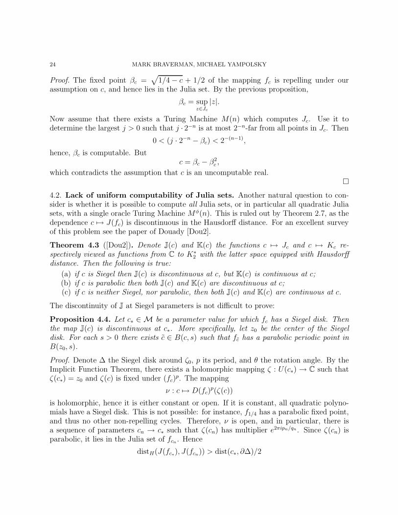
24 MARK BRAVERMAN, MICHAEL YAMPOLSKY
Proof. The fixed point βc =√
1/4− c + 1/2 of the mapping fc is repelling under ourassumption on c, and hence lies in the Julia set. By the previous proposition,
βc = supz∈Jc
|z|.
Now assume that there exists a Turing Machine M(n) which computes Jc. Use it todetermine the largest j > 0 such that j · 2−n is at most 2−n-far from all points in Jc. Then
0 < (j · 2−n − βc) < 2−(n−1),
hence, βc is computable. Butc = βc − β2
c ,
which contradicts the assumption that c is an uncomputable real.
4.2. Lack of uniform computability of Julia sets. Another natural question to con-sider is whether it is possible to compute all Julia sets, or in particular all quadratic Juliasets, with a single oracle Turing Machine Mφ(n). This is ruled out by Theorem 2.7, as thedependence c 7→ J(fc) is discontinuous in the Hausdorff distance. For an excellent surveyof this problem see the paper of Douady [Dou2].
Theorem 4.3 ([Dou2]). Denote J(c) and K(c) the functions c 7→ Jc and c 7→ Kc re-spectively viewed as functions from C to K∗
2 with the latter space equipped with Hausdorffdistance. Then the following is true:
(a) if c is Siegel then J(c) is discontinuous at c, but K(c) is continuous at c;(b) if c is parabolic then both J(c) and K(c) are discontinuous at c;(c) if c is neither Siegel, nor parabolic, then both J(c) and K(c) are continuous at c.
The discontinuity of J at Siegel parameters is not difficult to prove:
Proposition 4.4. Let c∗ ∈ M be a parameter value for which fc has a Siegel disk. Thenthe map J(c) is discontinuous at c∗. More specifically, let z0 be the center of the Siegeldisk. For each s > 0 there exists c ∈ B(c, s) such that fc has a parabolic periodic point inB(z0, s).
Proof. Denote ∆ the Siegel disk around ζ0, p its period, and θ the rotation angle. By theImplicit Function Theorem, there exists a holomorphic mapping ζ : U(c∗) → C such thatζ(c∗) = z0 and ζ(c) is fixed under (fc)
p. The mapping
ν : c 7→ D(fc)p(ζ(c))
is holomorphic, hence it is either constant or open. If it is constant, all quadratic polyno-mials have a Siegel disk. This is not possible: for instance, f1/4 has a parabolic fixed point,and thus no other non-repelling cycles. Therefore, ν is open, and in particular, there isa sequence of parameters cn → c∗ such that ζ(cn) has multiplier e2πipn/qn. Since ζ(cn) isparabolic, it lies in the Julia set of fcn . Hence
distH(J(fc∗), J(fcn)) > dist(c∗, ∂∆)/2
COMPUTABILITY OF JULIA SETS 25
for n large enough.
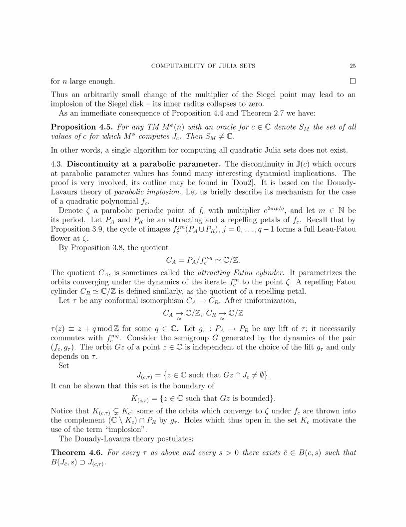
Thus an arbitrarily small change of the multiplier of the Siegel point may lead to animplosion of the Siegel disk – its inner radius collapses to zero.
As an immediate consequence of Proposition 4.4 and Theorem 2.7 we have:
Proposition 4.5. For any TM Mφ(n) with an oracle for c ∈ C denote SM the set of allvalues of c for which Mφ computes Jc. Then SM 6= C.
In other words, a single algorithm for computing all quadratic Julia sets does not exist.
4.3. Discontinuity at a parabolic parameter. The discontinuity in J(c) which occursat parabolic parameter values has found many interesting dynamical implications. Theproof is very involved, its outline may be found in [Dou2]. It is based on the Douady-Lavaurs theory of parabolic implosion. Let us briefly describe its mechanism for the caseof a quadratic polynomial fc.
Denote ζ a parabolic periodic point of fc with multiplier e2πip/q, and let m ∈ N beits period. Let PA and PR be an attracting and a repelling petals of fc. Recall that byProposition 3.9, the cycle of images f jm
c (PA∪PR), j = 0, . . . , q−1 forms a full Leau-Fatouflower at ζ .
By Proposition 3.8, the quotient
CA = PA/fmqc ≃ C/Z.
The quotient CA, is sometimes called the attracting Fatou cylinder. It parametrizes theorbits converging under the dynamics of the iterate fm
c to the point ζ . A repelling Fatoucylinder CR ≃ C/Z is defined similarly, as the quotient of a repelling petal.
Let τ be any conformal isomorphism CA → CR. After uniformization,
CA 7→≈
C/Z, CR 7→≈
C/Z
τ(z) ≡ z + qmod Z for some q ∈ C. Let gτ : PA → PR be any lift of τ ; it necessarilycommutes with fmq
c . Consider the semigroup G generated by the dynamics of the pair(fc, gτ ). The orbit Gz of a point z ∈ C is independent of the choice of the lift gτ and onlydepends on τ .
SetJ(c,τ) = z ∈ C such that Gz ∩ Jc 6= ∅.
It can be shown that this set is the boundary of
K(c,τ) = z ∈ C such that Gz is bounded.Notice that K(c,τ) ( Kc: some of the orbits which converge to ζ under fc are thrown intothe complement (C \ Kc) ∩ PR by gτ . Holes which thus open in the set Kc motivate theuse of the term “implosion”.
The Douady-Lavaurs theory postulates:
Theorem 4.6. For every τ as above and every s > 0 there exists c ∈ B(c, s) such thatB(Jc, s) ⊃ J(c,τ).

26 MARK BRAVERMAN, MICHAEL YAMPOLSKY
Figure 6. Before and after a parabolic implosion. The Julia sets (black)and filled Julia sets (light gray) of a parabolic quadratic f1/4 (left), and off1/4+ǫ for a small complex ǫ.
Thus the Julia set of fc grows “bigger” under the perturbation from c to c.
5. Positive results
5.1. Computability of filled Julia sets. In this section we show:
Theorem 5.1. For any polynomial p(z) there is an oracle Turing Machine Mφ(n) thatgiven an oracle access to the coefficients of p(z), outputs a 2−n-approximation of the filledJulia set Kp ≡ K(p(z)).
Moreover,
Theorem 5.2. In the case when p(z) = z2 + c is quadratic, only two oracle machinessuffice to compute all non-parabolic filled Julia sets: one for c ∈M, and one for c /∈M.
Theorem 5.1 answers in the affirmative the question posed to us by J. Milnor, after we firstdemonstrated the existence of non-computable quadratic Julia sets in [BY].
Let us first formulate a general fact:
Proposition 5.3. Let Q(z) be a complex polynomial. Then there exists a Turing MachineMφ with an oracle input for the coefficients of Q(z) such that the following holds. Considerany dyadic ball B = B(x, r) ⊂ C, x ∈ D2, r ∈ D, and let α1, . . . , αm be the roots of Q(z)contained in B. For any natural number n, the machine Mφ will take n, r, and x as inputs,

COMPUTABILITY OF JULIA SETS 27
and will output a finite sequence of complex numbers β1, . . . , βk with dyadic rational realand imaginary parts for which:
• βi ∈ B(x, r + 2−n);• each βi lies at a distance not more than 2−n from some root of Q(z);• for every αj there exists βi with |αj − βi| < 2−n.
For a classical reference, see [Wey]; a review of modern approaches to iterative root findingalgorithms may be found in [BCSS].
For a given polynomial p(z) we construct a machine computing the corresponding filledJulia set Kp. We will use some combinatorial information about p in the construction, sothe algorithm will, in general, vary with the polynomial. Note that all the information wewill need can be encoded using a finite number of bits.
• Information that would allow us to compute the non-repelling orbits of the polyno-mial with an arbitrary precision, as well as their type: attracting, parabolic, Siegel,or Cremer. By Fatou-Shishikura bound, there are at most deg p− 1 of them.
By Proposition 5.3, such information could, for example, consist of the list ofperiods ki of such orbits; and for each i a finite collection of dyadic balls Dj
i kij=1
separating the points of the corresponding orbit from the other solutions of theequation pki(z) = z.• For each (super)attracting periodic orbit ζ = ζ1, . . . , ζk, a finite union of dyadic
balls Dζ = ∪B(ζi, ri) with the property
pk(Dζ) ⋐ Dζ.
• For each parabolic periodic point with period m and multiplier p/q, the values ofm, p, q.• In the case of a Siegel disc D, information that would allow us to identify a re-
pelling periodic point ζD in the same connected component of Kp as D. Again, byProposition 5.3, it is sufficient to know its period, and a small enough dyadic ballaround it, which separates it from all other points, periodic with the same period.
5.2. Computing Kp. We are given a dyadic point d ∈ D and an n ∈ N. Our goal is toalways terminate and output 1 if B(d, 2−n)∩Kp 6= ∅ and to output 0 if B(d, 2·2−n)∩Kp = ∅.We do it by constructing five machines. They are guaranteed to terminate each on adifferent condition, always with a valid answer. Together they cover all the possible cases.
Lemma 5.4. There are five oracle machines Mext, Mjul, Mattr, Mpar, Msieg such that
(1) if d is at distance ≥ 43· 2−n from Kp, Mext(d, n) will halt and output 0. If d is at
distance ≤ 2−n from Kp, Mext(d, n) will never halt;(2) if d is at distance ≤ 5
3· 2−n from Jp, Mjul(d, n) will halt and output 1. If d is at
distance ≥ 2 · 2−n from Jp, Mjul(d, n) will never halt;(3) Mattr(d, n) halts and outputs 1 if and only if d is inside the basin of an attracting
orbit of p;

28 MARK BRAVERMAN, MICHAEL YAMPOLSKY
(4) Mpar(d, n) halts and outputs 1 if and only if d is inside the basin of a parabolic orbitof p;
(5) Msieg(d, n) halts and outputs 1 if the orbit of d reaches a Siegel disc, and d is atdistance ≥ 4
3· 2−n from Jp. It never halts if d is at distance ≥ 2 · 2−n from Kp.
Proof of Theorem 5.1, given Lemma 5.4. By Fatou-Sullivan classification it is clear that foreach (d, n) at least one of the machines halts. Moreover, by the definition of the machines,they always output a valid answer whenever they halt. Hence running the machines inparallel and returning the output of the first machine to halt gives the algorithm forcomputing Kp.
We now prove Lemma 5.4.
Proof. (of Lemma 5.4) We give a simple construction for each of the five machines.
(1) Mext: Take a large ball B such that p−1(B) ⋐ B. Intuitively, we pull the ball backunder p to get a good approximation of Kp. Let Bk be a 2−(n+3)-approximation ofthe set p−k(B). Output 0 iff Bk ∩ B(d, 7
6· 2−n) = ∅. It is not hard to see that this
algorithm satisfies the conditions on Mext.(2) Mjul: By Proposition 5.3 for each k we can compute all periodic orbits of p(z) in
B with periods j ≤ k, as roots of the equation
pj(z)− z = 0
with an arbitrarily high precision. Moreover, by our assumptions, we have themeans to distinguish the non-repelling orbits from the repelling ones.
Let Ck be a finite collection of complex numbers with dyadic rational real andimaginary parts which approximate the repelling periodic orbits with periods up tok with precision 2−(n+3). Output 1 iff d(d, Ck) <
116· 2−n. The repelling periodic
orbits are all in Jp and are dense in this set. Hence the algorithm satisfies theconditions on Mjul.
(3) Mattr : For each attracting orbit ζ of period mζ find lζ such that
B(pmζ (Dζ), 2−lζ) ⊂ Dζ .
Letl = 1 + sup lζ , and m =
∏mζ .
Let zk be a 2−(l+3)-approximation of pmk(d). If d is inside the basin of an attractingorbit ζ, then zk will be inside Dζ for some k. Output 1 if zk is inside Dζ and at
least 2−l-far from the boundary of Dζ .(4) Mpar: We make use of Lemma 3.7. Since we can produce arbitrarily good approxi-
mations of every parabolic periodic point ζ of p(z), we do not need an oracle for the
value of this point. Let Lζk be the sets from Lemma 3.7 corresponding to the point
ζ . Let zk = pk(d) computed with precision 2−(k+2). We output 1 if zk is inside Lζk
for some ζ and at least 2−k-away from its boundary.

COMPUTABILITY OF JULIA SETS 29
(5) Msieg: This is the most interesting case. It is not hard to see that for each k, wecan compute a union Ek of dyadic balls such that
k⋃
i=0
pi
(B(d,
4
3· 2−n)
)⊂ Ek ⊂
k⋃
i=0
pi
(B(d,
5
3· 2−n)
).
Let ζ∗ be the center of the Siegel disc (one of the centers, in case of an orbit), andlet y be the given periodic point in the connected component of ζ∗. We terminateand output 1 if Ek separates ζ∗ from y in C (or covers either one of them) for somek.
Clearly, if d is inside the Siegel disc, then the forward images of B(d, 43· 2−n) will
cover an annulus in the disc that will separate ζ∗ from the boundary of the disc,and in particular from y. Hence Msieg will terminate and output 1.
On the other hand, if the distance from d to Kp is ≥ 2 · 2−n, then Ek ∩Kp = ∅for all k. In particular, Ek cannot separate ζ∗ from y, since they are connected inKp.
The proof is simplified in the case of a quadratic polynomial.
Proof of Theorem 5.2. . If we assume that p(z) = fc(z) then by the Fatou-Shishikurabound, there is at most one non-repelling orbit. By our assumption, it is not parabolic.Moreover, if it is a Siegel orbit, then the Julia set is connected. Therefore, any repellingperiodic orbit will be in the same connected component of Kp as the Siegel disk.
If c /∈ M, we run Mext and Mjul. One and only one of them is guaranteed to halt andoutput a correct answer.
For c ∈ M we will use a modified Turing Machine Msieg. It will compute the set Ek asbefore. If Ek separates the plane, it will use Proposition 5.3 to search for a periodic pointof period at most k both in the exterior and the interior components of Ek. If a k is foundfor which such two orbits are located, or if Ek covers a periodic orbit, it will terminate andoutput 1.
If c ∈M, then we run Mext, Mjul, Mhyp, and Msieg. As before, it is easy to see that oneof them will terminate, and its output will be a correct one.
Corollary 5.5. Denote by P the set of c’s for which Jc is parabolic. The function K : c 7→Kz2+c is continuous in the Hausdorff metric on the set M\P.
5.3. Computability of Julia sets in the absense of rotation domains. Similar ideaswere used in [BBY1] to prove the following theorem:
Theorem 5.6. Let f be a rational map f : C → C without rotation domains. Then itsJulia set is computable in the spherical metric by an oracle Turing machine Mφ with theoracle representing the coefficients of f . The algorithm uses the following non-uniforminformation about each parabolic periodic point ζ of f with period m and multiplier e2πip/q:

30 MARK BRAVERMAN, MICHAEL YAMPOLSKY
• a dyadic ball B(w, r) ∋ p such that B(w, 2r) does not contain any other pointsperiodic with period m;• the values of m, p, and q.
Proof. For every natural n we can compute a sequence of rationals qi such that
(5.1) B(Jf , 2−(n+2)) ⋐
∞⋃
i=1
B(qi, 2−(n+1)) ⋐ B(Jf , 2
−n).
To do that, for each k > n+2 we compute 2−k-approximations of the periodic points of fin C with periods at most k using Proposition 5.3. Let M > 0 be some bound on |D2fm(z)|in the area of an approximate periodic orbit ri with period m. Then |Dfm(ri)| > 1+2−kMimplies that |Dfm(w)| > 1 for the periodic point w which ri approximates. In this case weadd the point ri to our sequence of rationals. Clearly, for each repelling periodic point of fwe will eventually obtain in this way a rational point which approximates it with precisionat least 2−(n+3). Since such points are contained in Jf , and dense there, our sequence hasthe desired property.
Of course, we can similarly eventually find every attracting orbit ζ of f with an arbitraryprecision. In this case, we will compute a set Dζ for this orbit with the same properties asbefore. Set D = ∪ζDζ .
Finally, for each parabolic periodic point ζ of f let Lζk be the sets from Lemma 3.7. Set
Lk = ∪ζLζk.
We are now ready to present an algorithm to find a set Cm ∈ C with distH(Cm, Jf) < 2−m.Fix m ∈ N. Our algorithm to find Cm ∈ C works as follows. At the k-th step:
• compute the finite union Bk = ∪ki=1B(qi, 2
−(m+1)) ∈ C;• compute with precision 2−(m+3) the complement of the preimage
f−k(D ∪ Lk),
that is, find Wk ∈ C such that
dH(Wk, C \ (f−k(D ∪ Lk))) < 2−(m+3);
• if Wk ⊂ Bk output Cm = Bk and terminate. Otherwise, go to step k + 1.
By Fatou-Sullivan classification, the algorithm will eventually terminate. Now supposethat the algorithm terminates on step k. Since Wk ⊂ Bk and Jf ⊂ B(Wk, 2
−(m+3)) we haveJf ⊂ B(Cm, 2
−(m+3)). On the other hand, ∪qi ⊂ Jf , and thus Bk = Cm ⊂ B(Jf , 2−(m+1)).
6. Computability of Julia sets of Siegel quadratics and negative results
6.1. Computabilty of r(θ) is equivalent to computability of Jθ. . Recall the dis-cussion of the family Pθ(z) = z2 + e2πiθz from §3.3. As before, if θ is a Brjuno number,we denote ∆θ its Siegel disk, and r(θ) the conformal radius of ∆θ. When θ /∈ B, we setr(θ) = 0. Let us denote rsup = sup r(θ). We let Jθ stand for J(Pθ).

COMPUTABILITY OF JULIA SETS 31
Of course, the change in parametrization from c to θ makes it natural to talk aboutcomputabilty of Jθ by a TM with an oracle for θ, rather than for c. However, these notionsare obviously equivalent, as c = c(θ) is found by the formula:
(6.1) c = c(θ) = λ/2− λ2/4, where λ = e2πiθ.
To address the question of computability of Jθ for θ ∈ B we first make note of thefollowing result, proven in [BBY1]:
Proposition 6.1. Suppose rθ is computable by a Turing Machine Mφ with an oracle forθ. Then so is Jθ.
To clarify the logic of the argument, let us break the proof into two steps:
Lemma 6.2. Suppose rθ is computable by a Turing Machine Mφ with an oracle for θ.Then so is the inner raidus ρ(∆θ, 0) ≡ ρθ.
Proof. The algorithm works as follows:
(I) For k ∈ N compute a set Dk ∈ C which is a 2−m-approximation of the preimageP−k
θ (D), for some sufficiently large disk D;(II) evaluate the conformal radius r(Dk, 0) with precision 2−(m+1) (this can be done,
for example, by using one of the numerous existing methods for computing theRiemann Mapping of a computable domain, see [BB]);
(III) as before, denote
F (x) = 4x/(1 + x)2, for x ∈ [0, 1].
Note that this function is monotone, and let ψ(w) = F−1(w). This function iscomputable, and ψ(1) = 1.
Evaluatep = ψ(rθ/r(Dk, 0))
with precision 2−(m+5)/ρ(D, 0). If
|1− p| < 2−(m+3)/ρ(D, 0),
then compute the inner radius ρ(Dk, 0) ≡ rk around 0 with precision 2−(m+1) andoutput this number. Else, increment k and return to step (I).
Termination. Let K = K(Pθ) be the filled Julia set of Pθ. Then
∩∞k=0Dk = K ⊃ ∆θ
and D0 ⊃ D1 ⊃ D2 ⊃ . . ..Hence for every δ > 0 there will be a step k = k(ǫ) after which
dist(∂Dk, Jθ) < δ.
Since ∂∆θ ⊂ Jθ, by Lemma 3.21 this implies that
|r(Dk, 0)− r(∆θ, 0)| = |r(Dk, 0)− rθ| < 4√r(D, 0)
√δ −→
δ→00.

32 MARK BRAVERMAN, MICHAEL YAMPOLSKY
Since for every large enough k, the value of
ψ(rθ/r(Dk, 0)) > 1− 2−(m+4)/ρ(D, 0),
the algorithm will eventually terminate on step (III).
Correctness. Now suppose the algorithm has terminated on step (III). As ∆θ ⊂ Dk,Lemma 3.21 implies that
1 ≥ ρθ
ρ(Dk, 0)≥ 1− 2−(m+1)
ρ(D, 0),
and so|ρ(Dk, 0)− ρθ| ≤ 2−(m+1).
Lemma 6.3. Suppose ρθ is computable by a Turing Machine Mφ with an oracle for θ.Then so is Jθ.
Proof. The algorithm to produce the 2−n approximation of the Julia set is the following.First, compute a large disk D around 0 with Pθ(D) ⋑ D. Then,
(I) compute a set Dk ∈ C which is a 2−(n+3)-approximation of the preimage P−kθ (D);
(II) set Wk to be the round disk with radius ρθ − 2−k about the origin. Compute a setBk ∈ C which is a 2−(n+3)-approximation of P−k
θ (Wk);(III) ifDk is contained in a 2−(n+1)-neighborhood ofBk, then output a 2−(n+1)-neighborhood
of Dk \Bk, and stop. If not, go to step (I).
A proof of the validity of the algorithm is obvious, and we leave it to the reader.
Figure 7. A figure produced by the algorithm of Lemma 6.3 for θ = (√
5−1)/2. It does not have the same artistic quality as Figure 4, but has aguaranteed accuracy up to the selected size of a pixel.
By Proposition 6.1 and Corollary 3.22 we have:
Theorem 6.4. The conformal radius r(θ) is computable by a Turing Machine with anoracle for θ if and only the same is true for the Julia set Jθ.

COMPUTABILITY OF JULIA SETS 33
Let us make a note:
Proposition 6.5. Let θ be of bounded type. Then Jθ is computable by a TM with an oraclefor θ.
Proof. By Proposition 3.18, ρθ is computable. The claim follows by Lemma 6.3.
Showing that there exist noncomputable Siegel Julia sets is much more delicate. In thenext section we will prove that this can happen even if θ itself is computable.
6.2. Conformal radius of a Siegel quadratic with a computable θ. The theorem weformulate below characterizes the values of r(θ) which correspond to computable parametersθ:
Theorem 6.6. Let r ∈ (0, rsup) be a real number. Then r = r(θ) is the conformal radiusof a Siegel disc of the Julia set Jθ for some computable number θ if and only if r is right-computable.
Before proving this theorem, let us formulate a corollary:
Corollary 6.7. There exist computable values of parameter c, such that the Julia set Jc isnot computable by a TM Mφ with an oracle access to c.
Proof. By Proposition 2.2 there exist right computable numbers r∗ ∈ [0, rsup] which arenot in RC . By Theorem 6.6, r∗ = r(θ∗) for θ∗ ∈ RC. Since θ∗ itself is computable, r∗ isuncomputable by a TM with an oracle access to θ∗. By Theorem 6.4, the Julia set Jθ∗ isuncomputable by a TM with an oracle access to θ∗. The claim follows by (6.1).
Proof of the “only if” direction of Theorem 6.6. We assume that θ is computable, and showthat r(θ) is right-computable. Recall that periodic orbits are dense in the Julia set Jθ. LetHn be the union of all repelling periodic orbits with periods between 1 and n. By Propo-sition 5.3 we can algorithmically find an arbitrarily good approximation of Hn by dyadicrationals.Jθ is connected, and ∪Hn is dense in Jθ. Thus for every l, there exists nl such that the
set B(Hj, 2−(l+1)) is connected. Moreover, such nl can be found algorithmically.
Since Jθ separates α from∞, the same is true for B(Hnl, 2−(l+1)) provided l is sufficiently
large. Hence we can compute a strictly increasing sequence nl∞l=l0⊂ N, and a set Ul ⊂ C
with the property
B(Hnl, 2−(l+1)) ⊂ Ul ⊂ B(Hnl
, 2−l).
such that C \ Ul has a simply-connected component Wl containing α.Using any constructive algorithm for computing the conformal radius [BB] we can ap-
proximate the k-th term of the sequence
Rk = r(B(Wk, 2−(k−1)), α) + 5 · 24− k−1
2

34 MARK BRAVERMAN, MICHAEL YAMPOLSKY
Hn → Jθ in Hausdorff metric and nk → ∞, thus by Lemma 3.21, Rk → r(θ). Moreover,Rk is a non-increasing sequence. Let ρk be a dyadic approximation ofRk that we computeso that |ρk −Rk| < 2−k. Let
rk = ρk + 3 · 2−k.
Then rk is a computable sequence of dyadic numbers. We have
limk→∞
rk = limk→∞
ρk = limk→∞
Rk = r(θ),
and for each k,
rk = ρk + 3 · 2−k ≥ Rk + 2 · 2−k ≥ Rk+1 + 4 · 2−(k+1) ≥ ρk+1 + 3 · 2−(k+1) = rk+1.
This shows that r(θ) is right-computable.Note that we know that Hn → Jθ is Hausdorff metric, which allows us to conclude
that rk → r(θ). However, we do not have (and cannot have) an estimate on the rate ofconvergence of Hn to Jθ, and thus cannot obtain an estimate on the rate of convergence ofrk → r(θ) and compute r(θ).
Proof of the “if” direction of Theorem 6.6. Given a computable sequence rn suchthat rn ց r we claim that we can construct a θ such that r = r(θ). We will be usingthe following three lemmas. The first one is Lemma 3.1 of [BY], and the second one isLemma 4.2 of [BBY2]. The proofs are outlined in Appendix B.
Lemma 6.8. For any initial segment I = [a0, a1, . . . , an], write ω = [a0, a1, . . . , an, 1, 1, 1, . . . ].Then for any ε > 0, there is an m > 0 and an integer N such that if we write β =[a0, a1, . . . , an, 1, 1, . . . , 1, N, 1, 1, . . .], where the N is located in the n+m-th position, then
Φ(ω) + ε < Φ(β) < Φ(ω) + 2ε.
Lemma 6.9. For ω as above, for any ε > 0 there is an m0 > 0, which can be computed from(a0, a1, . . . , an) and ε, such that for any m ≥ m0, and for any tail I = [an+m, an+m+1, . . .]if we denote
βI = [a1, a2, . . . , an, 1, 1, . . . , 1, an+m, an+m+1, . . .],
thenΦ(βI) > Φ(ω)− ε.
Lemma 6.10. Let ω = [a1, a2, . . .] be a Brjuno number, that is Φ(ω) < ∞. Denoteωk = [a1, a2, . . . , ak, 1, 1, . . .]. Then for every ε > 0 there is an m such that for all k ≥ m,
Φ(ωk) < Φ(ω) + ε.
Using Proposition 6.5, we can get a computable version of Lemmas 6.8 and 6.9.
Lemma 6.11. For any given initial segment I = [a0, a1, . . . , an] and m0 > 0, write ω =[a0, a1, . . . , an, 1, 1, 1, . . . ]. Then for any ε > 0, we can uniformly compute m > m0, aninteger t and an integer N such that if we write β = [a0, a1, . . . , an, 1, 1, . . . , 1, N, 1, 1, . . .],where the N is located in the n +m-th position, we have
(6.2) r(ω)− 2ε < r(β) < r(ω)− ε,

COMPUTABILITY OF JULIA SETS 35
(6.3) Φ(β) > Φ(ω),
and for any
γ = [a0, a1, . . . , an, 1, 1, . . . , 1, N, 1, . . . , 1, cn+m+t+1, cn+m+t+2, . . .],
(6.4) Φ(γ) > Φ(ω)− 2−n.
Proof. We first show that such m and N exist, and then give an algorithm to computethem. By Lemma 6.8 we can increase Φ(ω) by any controlled amount by modifying oneterm arbitrarily far in the expansion.
By Theorem 3.13, f : θ 7→ Φ(θ) + log r(θ) extends to a continuous function. Hence forany ε0 there is a δ such that |f(x)− f(y)| < ε0 whenever |x− y| < δ. In particular, thereis an m1 such that |f(β)− f(ω)| < ε0 whenever m ≥ m1.
This means that if we choose m large enough, a controlled increase of Φ closely corre-sponds to a controlled drop of r by a corresponding amount, hence there are m > m0 andN such that (6.2) holds. (6.3) is satisfied almost automatically. The only problem is tocomputably find such m and N .
To this end, we apply Proposition 6.5. Together with Theorem 6.4, it implies that forany specific m and N we can compute r(β). This means that we can find the suitable mand N , by enumerating all the pairs (m,N) and exhaustively checking (6.2) and (6.3) forall of them. We know that eventually we will find a pair for which (6.2) and (6.3) hold.
Finally, t exists and can be computed by Lemma 6.9.
Lemma 6.10 yields the following lemma.
Lemma 6.12. The supremum of r(θ) over all angles is equal to the supremum over theangles whose continued fraction expansion has only finitely many terms that are not 1:
rsup = supθ=[a1,a2,...,ak,1,1,...]
r(θ).
Proof. Let ε > 0 be an arbitrary small positive number. By the definition of rsup there isa θ = [a1, a2, . . .] such that log r(θ) > log rsup − ε. Denote
θk = [a1, a2, . . . , ak, 1, 1, . . .].
Lemma 6.10 states that there is an m such that for k ≥ m, Φ(θk) < Φ(θ) + ε. Moreover,there is a δ such that whenever |φ− θ| < δ we have |υ(φ)− υ(θ)| < ε.θk → θ, hence there is an n ≥ m such that |θn − θ| < δ. θn has the required form, and
we have
log r(θn) = υ(θn)− Φ(θn) > υ(θ)− Φ(θ)− 2ε = log r(θ)− 2ε > log rsup − 3ε.
This shows that we can make r(θn) as close to rsup as we like.
We are given r = lim ց rn < rsup, hence there is an s and an ε > 0 such thatrs < rsup−2ε. By Lemma 6.12, there is a γ0 = [a1, a2, . . . , an, 1, 1, . . .] such that rs + ε/2 <r(γ0) < rs + ε.

36 MARK BRAVERMAN, MICHAEL YAMPOLSKY
We are now ready to give an algorithm for computing a rotation number θ for whichr(θ) = lim ց rn. The algorithm works as follows. On stage k it produces a finite initialsegment Ik = [a0, . . . , amk
] such that the following properties are maintained:
(1) I0 = [a1, a2, . . . , an];(2) Ik has at least k terms, i.e. mk ≥ k;(3) for each k, Ik+1 is an extension of Ik;(4) for each k, denote γk = [Ik, 1, 1, . . .], then rs+k + 2−(k+1)ε < r(γk) < rs+k + 2−kε;(5) for each k, Φ(γk) > Φ(γk−1);(6) for each k, for any extension
β = [Ik, bmk+1, bmk+2, . . .],
Φ(β) > Φ(γk)− 2−k.
The first three properties are very easy to assure. The last three are maintained usingLemma 6.11. By this Lemma we can decrease r(γk−1) by any given amount (possibly inmore than one step) by extending Ik−1 to Ik. Here we use the facts that the rk’s arecomputable and non-increasing.
Denote θ = limk→∞ γk. The continued fraction expansion of θ is the limit of the initialsegments Ik. This algorithm gives us at least one term of the continued fraction expansion ofθ per iteration, hence we would need at most O(n) iterations to compute θ with precision2−n (in fact, much fewer iterations would suffice). The initial segment γ0 can also becomputed as in the proof of Lemma 6.11. It remains to prove that, in fact, θ is the rotationnumber we are looking for.
Lemma 6.13. The following equalities hold:
Φ(θ) = limk→∞
Φ(γk) and r(θ) = limk→∞
r(γk) = r.
Proof. By the construction, the limit θ = lim γk exists. We also know that the sequencer(γk) converges to the number r = lim ց rk, and that the sequence Φ(γk) is monotonenon-decreasing, and hence converges to a value ψ (a priori we could have ψ = ∞). Bythe Caratheodory Kernel Theorem, we have r(θ) ≥ r > 0, so Φ(θ) < ∞. On the otherhand, by the property we have maintained through the construction, we know that Φ(θ) >Φ(γk)− 2−k for all k. Hence Φ(θ) ≥ ψ. In particular, ψ <∞.
From [BC2] we know that
(6.5) ψ + log r = lim(Φ(γk) + log r(γk)) = Φ(θ) + log r(θ).
Hence we must have ψ = Φ(θ), and r = r(θ), which completes the proof.
7. Interpretation of the results
7.1. How difficult is it to produce a θ for which Jθ is uncomputable? As we haveseen, a value of θ for which Jθ is uncomputable can be produced constructively. As we willsee below, under a reasonable assumption, it is not even hard to do so:
COMPUTABILITY OF JULIA SETS 37
Conditional Implication. Assume that the 1-periodic continuous function υ : θ 7→ Φ(θ)+log r(θ) has a computable modulus of continuity (2.1); this follows, for instance, fromMarmi-Moussa-Yoccoz Conjecture. Suppose there is a computable sequence r1, r2, . . . ofdyadic numbers such that
• ri is non-increasing, r1 ≥ r2 ≥ . . ., and• limi→∞ ri = r.
Then there is a poly-time computable θ (and hence a poly-time computable c = c(θ)) suchthat r(θ) = r.
Proof. By the assumption, there is a computable function µ : N→ N such that
|υ(θ1)− υ(θ2)| < 2−n whenever |θ1 − θ2| < 2−µ(n).
The proof goes along the lines of the proof of the “if” direction of Theorem 6.6. Weoutline the modifications made to the proof here and leave the details to the reader. Thekey difference is that in the proof of Theorem 6.6 we used Lemma 6.11 to perform a step indecreasing the conformal radius from r(γk−1) to r(γk). The algorithm there is basically anexhaustive search, which, of course, could take much longer than polynomial time in theprecision of γk to compute. By assuming that υ has a computable modulus of continuity,we can deal with Φ(γk−1) and Φ(γk) instead of the r(•)’s. We have an explicit formula forΦ that converges well, and we can compute the continued fractions coefficients to makeΦ(γk) close to whatever we want relatively fast.
The step of going from γk−1 to γk is as follows. First, we do the following computations:
• compute dk which is the “drop” in r we are trying to achieve; we want
dk/2 < log(r(γk−1))− log(r(γk)) < dk;
• compute using the function µ a value δk such that |υ(x)− υ(y)| < dk/8 whenever|x− y| < δk.
We have no a priori bound on how long these computations would take, but we would stilllike to be computing θ in polynomial time. To achieve this, we use 1’s in the continuedfraction expansion of θ to “pad” the computation.
When asked about the value of θ with precision 2−n which is higher than what the knownterms of the expansion [Ik−1] can provide, we do the following:
• try to compute dk and δk as above, but run the computation for at most n steps;• if the computation does not terminate, output an answer consistent with the initial
segment [Ik−1, 1, 1, . . . , 1︸ ︷︷ ︸2n
];
• if the computation terminates in less than n steps proceed as described below.
Note that so far the computation is polynomial in n. For some sufficiently large n thecomputation will terminate in n steps, at which point we will have computed dk and δk. Ifnecessary, we then add more 1’s to the initial segment to assure that |γk−1 − γk| < δk.

38 MARK BRAVERMAN, MICHAEL YAMPOLSKY
Recall that our goal is to assure that
dk/2 < log(r(γk−1))− log(r(γk)) < dk.
With the current initial segment for γk we have |γk−1−γk| < δk, and hence in the difference
log(r(γk−1))− log(r(γk)) = Φ(γk)− Φ(γk−1) + (υ(γk−1)− υ(γk))
the last term is bounded by dk/8. This means that for the current step it suffices to increaseΦ(γk) relative to Φ(γk−1) by between 5
8dk and 7
8dk.
Let M be the total length of Ik−1 and the 1’s we have added, and let us extend thecontinued fraction by putting N ∈ N in the M + 1-st term, and all 1’s further. IncreasingM if necessary, we can ensure an approximate equality
Φ(γk) ≈ Φ(γk−1) + α(N) logN
up to an error of 132dk. Let pM/qM be the M-th convergent of the resulting continued
fraction. Recall that on an input n we need to compute θ with precision 2−n in timepolynomial in n. If 2−n > 1/
√qM , then we do not need to know anything about N to
compute the required approximation. Suppose 2−n < 1/√qM , which means n > log qM/2.
And we have time polynomial in log qM to perform the computation.Note that M = O(log qM ). It is also not hard to see that α(N) < 2−M/2, so in order
to have a change by ≈ 3dk/4 we must have N > eΩ(2M/2), hence by making M sufficiently
large (depending on the value of dk), we can guarantee that N > e2M/3
. This means thatwe can approximate α(N) with the truncated function Φ at the M-th convergent of thecontinued fraction. Write pM/qM = [a1, a2, . . . , aM ], and denote
β = [a1, a2, . . . , aM ] · [a2, a3, . . . , aM ] · . . . · [aM−1, aM ] · [aM ].
Then β approximates α(N) within a very small relative error. In particular, we can assurethat
β ·(
1− 1
32
)< α(N) < β ·
(1 +
1
32
).
In time polynomial in log qM we can compute the exact expression for β using rationalarithmetic: β = p/q. Now we can estimate N and write it as e6dk/8β in time polynomial inlog(qM). From there we can continue by adding enough 1’s to get Ik and γk = [Ik, 1, 1, . . .].By the construction, it would give us the necessary decrease in the value of r(γk).
7.2. Why is Kθ always computable? To provide some intuition why the filled Julia setis computable even when the Julia set is not, we propose the following toy model.
Let A : N→ 0, 1 be any uncomputable predicate. Consider the set
Ωt =
S1⋃
k∈N, dk=1
re2πi/k| r ∈ [1− 1k, 1] for t = (0.d1d2d3 . . .)2 ∈ [0, 1)
S1⋃
k∈N, A(k)=1
re2πi/k| r ∈ [1− 1k, 1] for t = 1

COMPUTABILITY OF JULIA SETS 39
To avoid ambiguity, we always take the finite expansion for dyadic t’s. An example of aset Ωt is depicted on Figure 8. Firstly, note that if t ∈ (0, 1) is not a computable real, thenthe set Ωt is non-computable by a TM without an oracle for t. Moreover, even for a TMMφ equipped with an oracle input for t, the set Ω1 is clearly non-computable. However,when filled, every Ωt becomes a computable set – the unit disk. This example suggeststhat filling an uncomputable Julia set we gain computability at the expense of losing thelong and narrow fjords of the Siegel disk.
Figure 8. Part of the picture of Ωt for t = (0.10101 . . .)2
7.3. What would a computer really draw? One thing is certain – it is unlikely todraw the true picture of an uncomputable Julia set. Indeed, by definition of computability,there is no systematic way of distinguishing the picture of Jc from all possible pictures ona screen with pixel size 2−n. The likelyhood of stumbling upon the correct image whenthe screen size is, say, 800x600 is very remote. The exact nature of the answer woulddepend, of course, on the specific algorithm being used. However, some insight is providedby considering the following problem, suggested to us by M. Shub.
Let J be the subset of C×C given by
J = (z, c) : z ∈ Jc.Shub has asked us:
Is the set J computable?
The answer again is “yes”:
Theorem 7.1. Let d > 0 be any computable real. Then the set
J ∩ C× B(0, d)
is a computable subset of C×C.

40 MARK BRAVERMAN, MICHAEL YAMPOLSKY
Informally, we may think of projection of J ∩ C × (c − ǫ, c + ǫ) to the first coordinate asthe picture that a computer could produce when Jc itself is uncomputable.
To understand how the mechanism of non-computability is destroyed in this case, con-sider again the set Ωt for t ∈ (0, 1] as the toy model. The set
W = (z, t) : z ∈ Ωt, t ∈ (0, 1] ⊂ C× R
is computable even though Ωt itself is non-computable for t = 1. This happens because inthe closure of W the “slice” corresponding to t = 1 is
S1⋃
k∈N
re2πi/k| r ∈ [1− 1
k, 1] ⊃ Ω1.
This set “masks” the computational hardness of Ω1, and makes W computable.
Computability of the set J. We prove Theorem 7.1 by showing that J is weakly com-putable (Definition 2.6).
We will need the following lemma.
Lemma 7.2. For any point (z, c) in the complement of the closure J, z converges to anattracting periodic orbit of fc : z 7→ z2 + c.
The proof of the lemma will require us to recall the nature of discontinuities in thefunction J(c), particularly the theory of parabolic implosion. We will give it in the end ofthe section.
The following lemma allows us to “cover” all points that belong to J.
Lemma 7.3. There is an algorithm A1(n) that on input n outputs a sequence of dyadicpoints p1, p2, . . . ∈ C×C such that
B(J, 2−(n+3)) ⊂∞⋃
j=1
B(pj , 2−(n+2)) ⊂ B(J, 2−(n+1)).
Proof. The repelling periodic orbits of fc are dense in Jc. Hence, the set
Srep = (z, c) : z is in a repelling periodic orbit of fcis dense in J. Srep is a union of a countable number of algebraic curves Sm
rep given by theconstraints
fmc (z) = z|(fm
c )′(z)| > 1
For each m we can compute a finite number of points pm1 , . . . , p
mrm
approximating Smrep such
that
B(Smrep, 2
−(n+3)) ⊂rm⋃
j=1
B(pmj , 2
−(n+2)) ⊂ B(Smrep, 2
−(n+1)).

COMPUTABILITY OF JULIA SETS 41
We have
J = Srep =∞⋃
m=1
Smrep.
Hence the computable sequence p11, . . . , p
1r1, p2
1, . . . , p2r2, . . . , pm
1 , . . . , pmrm, . . . satisfies the con-
ditions of the lemma.
Corollary 7.4. There is an oracle machine Mφ1,φ2
1 (n), where φ1 is an oracle for z ∈ C
and φ2 is an oracle for c ∈ C, such that Mφ1,φ2
1 always halts whenever d((z, c), J) < 2−(n+4)
and never halts if d((z, c), J) ≥ 2−n.
Proof. Query the oracles for a point p ∈ C× C such that d(p, (z, c)) < 2−(n+4). Then runthe following loop:
i← 0doi← i+ 1generate pi using A1(n) from Lemma 7.3
while d(p, pi) > 2−(n+2)
If d((z, c), J) < 2−(n+4), then d(p, J) < 2−(n+3), hence by Lemma 7.3 there is an i suchthat d(p, pj) ≤ 2−(n+2), and the loop terminates. If d((z, c), J) > 2−n, then d(p, J) >2−n − 2−(n−4) > 1.5 · 2−(n+1). Hence, by Lemma 7.3, p /∈ B(pi, 2
−(n+1)) for all i, and theloop will never terminate.
The following lemma allows us to exclude points outside J from J.
Lemma 7.5. There is an oracle machine Mφ1,φ2
2 , where φ1 is an oracle for z ∈ C and φ2
is an oracle for c ∈ C, such that Mφ1,φ2
2 halts if and only if z converges to an attractingperiodic orbit (or to ∞) under fc : z 7→ z2 + c.
Proof. M2 is systematically looking for an attracting cycle of fc. It also iterates fc on zwith increasing precision and for increasingly many steps until we are sure that either oneof the two things holds:
(1) the orbit of z converges to ∞; or(2) we find an attracting orbit of fc and the orbit of z converges to it.
If the search is done systematically, the machine will eventually halt if one of the possi-bilities above holds. It obviously won’t halt if neither holds.
Proof of Theorem 7.1. The algorithm is: Run the machines Mφ1,φ2
1 (n) from Corollary
7.4 and Mφ1,φ2
2 from Lemma 7.5 in parallel. Output 1 if M1 terminates first and 0 if M2
terminates first.First we observe that M1(n) only halts on points that are 2−n-close to J, in which case
1 is a valid answer according to Definition 2.6. Similarly, M2 only halts on points that areoutside J, in which case 0 is a valid answer. Hence if the algorithm terminates, it outputsa valid answer. It remains to see that it does always terminate. Consider two cases.

42 MARK BRAVERMAN, MICHAEL YAMPOLSKY
Case 1: (z, c) ∈ J. In this case d((z, c), J) = 0 < 2−(n+4), and the first machine isguaranteed to halt.
Case 2: (z, c) /∈ J. By Lemma 7.2, z converges to an attracting periodic orbit of fc inthis case, and hence the second machine is guaranteed to halt.
Proof of Lemma 7.2. Suppose z /∈ Jc and the orbit of z does not belong to an attractingbasin. By the Fatou-Sullivan classification (see e.g. [Mil]), there exists k ∈ N such thatw ≡ fk
c (z) belongs to a Siegel disk or to the immediate basin of a parabolic orbit. Ouraim is to show that for an arbitrary small δ > 0, there exists a pair (z, c) ∈ C × C with|z − z| < δ, |c− c| < δ, and for which z ∈ Jc. We will treat the Siegel case first.
The case when w lies in a Siegel disk. Let us denote ∆ the Siegel disk containing w, andlet m ∈ N be its period, that is, the mapping
fmc : ∆→ ∆
is conjugated by a conformal change of coordinates φ : ∆→ D to an irrational rotation ofD.
By Proposition 4.4, we have the following. Denote ζ = φ−1(0) ∈ ∆ the center of theSiegel disk. For each s > 0 there exists c ∈ B(c, s) such that fc has a parabolic periodic
point ζ of period m in B(ζ, s). In particular, Jc is connected, and B(ζ, s) ∩ Jc 6= ∅.Consider now the fm
c -invariant analytic circle
Sr = φ−1(z = re2πiθ, θ ∈ [0, 2π))which contains w. Let ǫ > 0 be such that
B(w, ǫ) ⊂ fkc (B(z, δ)) ∩∆.
Set B ≡ B(w, ǫ/2) and let n ∈ N be such that the union⋃
0≤i≤n
fmic (B) ⊃ Sr.
By Proposition 4.4 for all δ > 0 small enough, there exist c ∈ B(c, δ) for which Jc isconnected and there is a point of Jc inside the domain bounded by Sr. Since repellingperiodic orbits of fc are dense in ∂∆, again for δ small enough, there are points of Jc onthe outside of Sr as well, and so there exists a point ξ ∈ Jc ∩ Sr. By construction, thereexists j ∈ N such that f j
c (B(z, δ)) ∋ ξ. By invariance of Julia set, if c is close enough to cwe have B(z, δ) ∩ Jc 6= ∅, and the proof is complete.
The case when w lies in a parabolic basin. Denote ζ the parabolic periodic point of fc
whose immediate basin contains w, and let m ∈ N be its period. We employ the notationsof §4.3.
Recall, that by Theorem 4.6, for every s > 0 there exists c ∈ B(c, s) such that B(Jc, s) ⊃J(c,τ).

COMPUTABILITY OF JULIA SETS 43
Since ζ ∈ Jc, and Jc is connected, there exists a point u ∈ Jc ∩ PR. Let w ∈ CA be theorbit of w, and let u ∈ CR be the orbit of u. Choose the translation τ : CA → CR so thatτ(w) = u. Then J(c,τ) ∋ z, and the claim follows by Theorem 4.6.
Appendix A. Proof of Proposition 3.18
Siegel quadratic Julia of bounded type sets may be constructed by means of quasicon-formal surgery (cf. [Dou1]) on a Blaschke product
fγ(z) = e2πiτ(γ)z2 z − 3
1− 3z.
This map homeomorphically maps the unit circle T onto itself with a single (cubic) criticalpoint at 1. The angle τ(γ) can be uniquely selected in such a way that the rotation numberof the restriction ρ(fγ |T) = γ.
For each n, the points1, fγ(1), f 2
γ (1), . . . , f qn+1−1γ (1)
form the n-th dynamical partition of the unit circle. The following result is due to Swiatekand Herman (for the proof see e.g. Theorem 3.1 of [dFdM]):
Theorem A.1 (Universal real a priori bound). There exists an explicit constant B > 1independent of γ and n such that the following holds. Let γ ∈ R \Q and n ∈ N. Then anytwo adjacent intervals I and J of the n-th dynamical partition of fγ are B-commensurable:
B−1|I| ≤ |J | ≤ B|I|.Proposition A.2 ([He]). For each bounded type γ = [a0, . . . , ak, . . .] the Blaschke prod-uct fγ is K1-quasisymmetrically conjugate to the rotation Rγ : x 7→ x + γmod Z. The
quasisymmetric constant may be taken as K1 = (2 sup ai)10B2
.
Let us now consider the mapping Ψ which identifies the critical orbits of fγ and Pγ by
Ψ : f iγ(1) 7→ P i
γ(cγ).
We have the following (see, for example, Theorem 3.10 of [YZ]):
Theorem A.3 (Douady, Ghys, Herman, Shishikura). The mapping Ψ extends to aK-quasiconformal homeomorphism of the plane C which maps the unit disk D onto theSiegel disk ∆γ. The constant K may be taken as the quasiconformal dilatation of anyglobal quasiconformal extension of the K1-qs conjugacy of Proposition A.2. In particular,K ≤ 2K1.
Elementary combinatorics implies that each interval of the n-th dynamical partitioncontains at least two intervals of the (n + 2)-nd dynamical partition. This in conjunctionwith Theorem A.1 implies that the size of an interval of the (n+2)-nd dynamical partitionof fγ is at most τn where
τ =
√B
B + 1.

44 MARK BRAVERMAN, MICHAEL YAMPOLSKY
Hence, setting
Ωn = P iγ(cγ), i = 0, . . . , qn+2,
by Theorem A.3,
distH(Ωn, ∂∆γ) < Kτn.
Appendix B. Proof of Lemmas 6.8, 6.9 and 6.10
We present outlines of proofs for Lemmas 6.8, 6.9 and 6.10. The complete proofs of theintermediate lemmas can be found in [BBY2] and [BY]. For convenience, we restate thelemmas here:
Lemma 6.8 For any initial segment I = [a0, a1, . . . , an], write ω = [a0, a1, . . . , an,1, 1, 1, . . . ]. Then for any ε > 0, there is an m > 0 and an integer N such that if we writeβ = [a0, a1, . . . , an, 1, 1, . . . , 1, N, 1, 1, . . .], where the N is located in the n+m-th position,then
Φ(ω) + ε < Φ(β) < Φ(ω) + 2ε.
Lemma 6.9 For ω as above, for any ε > 0 there is an m0 > 0, which can becomputed from (a0, a1, . . . , an) and ε, such that for any m ≥ m0, and for any tail I =[an+m, an+m+1, . . .] if we denote
βI = [a1, a2, . . . , an, 1, 1, . . . , 1, an+m, an+m+1, . . .],
then
Φ(βI) > Φ(ω)− ε.Lemma 6.10 Let ω = [a1, a2, . . .] be a Brjuno number, that is Φ(ω) < ∞. Denote
ωk = [a1, a2, . . . , ak, 1, 1, . . .]. Then for every ε > 0 there is an m such that for all k ≥ m,
Φ(ωk) < Φ(ω) + ε.
Denote
Φ−(ω) = Φ(ω)− α0(ω)α1(ω) . . . αn+m−1(ω) log1
αm+n(ω).
The value of the integer m > 0 is yet to be determined. Denote
βN = (a0, a1, . . . , an, 1, 1, . . . , 1, N, 1, 1, . . .).
The following estimates are proven by induction.
Lemma B.1. For any N , the following holds:
(1) For i ≤ n +m we have∣∣∣∣log
αi(βN)
αi(βN+1)
∣∣∣∣ < 2i−(n+m)/N ;

COMPUTABILITY OF JULIA SETS 45
(2) for i < n +m, ∣∣∣∣logαi(β
N)
αi(β1)
∣∣∣∣ < 2i−(n+m);
(3) for i < n +m, ∣∣∣∣∣loglog 1
αi(βN )
log 1αi(βN+1)
∣∣∣∣∣ < 2i−(n+m)+1;
(4) for i < n +m− 1, ∣∣∣∣∣loglog 1
αi(βN )
log 1αi(β1)
∣∣∣∣∣ < 2i−(n+m)+1.
The estimates yield the following.
Lemma B.2. For any ω of the form as in lemma 6.8 and for any ε > 0, there is an m0 > 0such that for any N and any m ≥ m0,
|Φ−(βN)− Φ−(β1)| < ε
4.
Proof. (Sketch). The∑
in the expression for Φ(β1) converges, hence there is an m1 > 1such that the tail of the sum
∑i≥n+m1
α1α2 . . . αi−1 log 1αi< ε
16. It can be shown that
• for a sufficiently large m0 > m1, if m > m0, then for any N the influence on thesum of the “head” elements is very small:
∣∣∣∣∣
n+m1−1∑
i=1
α1(βN) . . . αi−1(β
N) log1
αi(βN)−
n+m1−1∑
i=1
α1(β1) . . . αi−1(β
1) log1
αi(β1)
∣∣∣∣∣ <ε
16;
• for the “tail” terms, for i ≥ n+m1 such that i 6= n +m,
α1(βN) . . . αi−1(β
N) log 1αi(βN )
α1(β1) . . . αi−1(β1) log 1αi(β1)
≤ e.
After the change each term of the tail could increase by a factor of e at most. The valueof the “tail” starts at the interval (0, ε
16], hence it remains in the interval (0, eε
16], and the
change in the tail is bounded by eε16< 3ε
16.
So the total change in Φ− is bounded by
change in the “head” + change in the “tail” <ε
16+
3ε
16=ε
4.
Lemma B.2 immediately yields:
Lemma B.3. For any ε and for the same m0(ε) as in lemma B.2, for any m ≥ m0 andN ,
|Φ−(βN)− Φ−(βN+1)| < ε
2.

46 MARK BRAVERMAN, MICHAEL YAMPOLSKY
Denote Φ1(ω) = α0(ω)α1(ω) . . . αn+m−1(ω) log 1αm+n(ω)
= Φ(ω) − Φ−(ω). Using the esti-
mates B.1 one can prove the following:
Lemma B.4. For sufficiently large m, for any N ,
Φ1(βN+1)− Φ1(βN) <ε
2.
Since Φ = Φ− + Φ1, summing the inequalities in Lemmas B.3 and B.4 yields:
Lemma B.5. For sufficiently large m, for any N ,
Φ(βN+1)− Φ(βN) < ε.
It is immediate from the formula of Φ(βN) that:
Lemma B.6.lim
N→∞Φ(βN ) =∞.
We are now ready to prove Lemma 6.8.
Proof of Lemma 6.8. Choose m large enough for lemma B.5 to hold. Increase N by oneat a time starting with N = 1. We know that Φ(β1) = Φ(ω) < Φ(ω) + ε, and by LemmaB.6, there exists an M with Φ(βM) > Φ(ω) + ε. Let N be the smallest such M . ThenΦ(βN−1) ≤ Φ(ω) + ε, and by lemma B.5
Φ(βN) < Φ(βN−1) + ε ≤ Φ(ω) + 2ε.
HenceΦ(ω) + ε < Φ(βN) < Φ(ω) + 2ε.
Choosing β = βN completes the proof.
The second part of the following Lemma follows by the same argument as Lemma B.2 bytaking N ≥ 1 to be an arbitrary real number, not necessairily an integer. The first part isobvious, since the tail of ω has only 1’s.
Lemma B.7. For an ω = β1 as above, for any ε > 0 there is an m0 > 0, such that forany m ≥ m0, and for any tail I = [an+m, an+m+1, . . .] if we denote
βI = [a1, a2, . . . , an, 1, 1, . . . , 1, an+m, an+m+1, . . .],
then ∑
i≥n+m
α1(β1)α2(β
1) . . . αi−1(β1) log
1
αi(β1)< ε,
andn+m−1∑
i=1
∣∣∣∣α1(βI) . . . αi−1(β
I) log1
αi(βI)− α1(β
1) . . . αi−1(β1) log
1
αi(β1)
∣∣∣∣ < ε.
We can now prove Lemma 6.9.

COMPUTABILITY OF JULIA SETS 47
Proof of Lemma 6.9. Applying lemma B.7 with ε2
instead of ε, we get
Φ(βI)− Φ(ω) =∑“head”(βI)− “head”(ω)+
∑“tail”(βI)− “tail”(ω) >
−ε2−
∑“tail”(ω) > −ε
2− ε
2= −ε.
Sketch of the proof of Lemma 6.10. We divide the sum for Φ(ω),
Φ(ω) =s∑
i=1
α1(ω) . . . αi−1(ω) log1
αi(ω)︸ ︷︷ ︸
“head”
+∞∑
i=s+1
α1(ω) . . . αi−1(ω) log1
αi(ω)︸ ︷︷ ︸
“tail”
,
so that “tail” < ε/16. Using the estimates from Lemma B.1 one can show that modifyingω to ωk for some appropriately chosen k ≫ s will satisfy:
•s∑
i=1
α1(ωk) . . . αi−1(ωk) log1
αi(ωk)<
s∑
i=1
α1(ω) . . . αi−1(ω) log1
αi(ω)+ ε/16,
since the relative error in the “head” terms can be made arbitrarily small;• for i > s,
α1(ωk) . . . αi−1(ωk) log1
αi(ωk)< 9 ·
s∑
i=1
α1(ω) . . . αi−1(ω) log1
αi(ω)+ 2−k/2.
Note that for i > k the 2−k/2 term alone dominates the expression on the left.
Finally for a k as above,
Φ(ωk) < “head”(ωk) + “tail”(ωk) < “head”(ω) + ε/16 + 9“tail”(ω) + 2−s+1 <
“head”(ω) + ε/16 + 9ε/16 + 2−s+1 < Φ(ω) + ε,
for a sufficiently large s.

48 MARK BRAVERMAN, MICHAEL YAMPOLSKY
References
[Ahl] L. Ahlfors. Lectures on Quasiconformal Mappings, Amer. Math. Soc., 2006.[ABC] A. Avila, X. Buff, A. Cheritat. Siegel disks with smooth boundaries. Acta Math. 193(2004), no.
1, 1–30.[BM] S. Banach, S. Mazur. Sur les fonctions caluclables. Ann. Polon. Math. 16(1937)[BBY1] I. Binder, M. Braverman, M. Yampolsky. Filled Julia sets with empty interior are computable.
e-print, math.DS/0410580. To appear in Journ. of FoCM.[BBY2] I. Binder, M. Braverman, M. Yampolsky. On computational complexity of Siegel Julia sets. Com-
mun. Math. Phys., 264(2006), no. 2, 317–334.[BB] E. Bishop, D.S. Bridges. Constructive Analysis. Springer-Verlag, Berlin (1985)[BCSS] L. Blum, F. Cucker, M. Shub, S. Smale, Complexity and Real Computation, Springer, New York,
1998.[BC1] X. Buff, A. Cheritat, Quadratic Siegel disks with smooth boudaries. Preprint Univ. Paul Sabatier,
Toulouse, III, Num. 242.[BC2] X. Buff, A. Cheritat, The Brjuno function continuously estimates the size of quadratic Siegel Disks,
Annals of Math. 164(2006), No. 1, 265-312.[Bru] A.D. Brjuno. Analytic forms of differential equations, Trans. Mosc. Math. Soc 25(1971)[Brv] M. Braverman, “Computational Complexity of Euclidean Sets: Hyperbolic Julia Sets are Poly-
Time Computable”, M. Sc. Thesis, University of Toronto, 2004, and Proc. CCA 2004, to appear.[Brv2] M. Braverman, On the complexity of real functions, Proc. 46 annual IEEE Symposium FOCS’05,
155-164.[Brv3] M. Braverman, Parabolic Julia Sets are Polynomial Time Computable. e-print math.DS/0505036.
To appear in Nonlinearity 19, 2006.[BrC] M. Braverman, S. Cook. Computing over the Reals: Foundations for Scientific Computing. Notices
of the AMS, 53(3), 2006.[BY] M. Braverman, M. Yampolsky. Non-computable Julia sets. Journ. Amer. Math. Soc. 19(2006), no.
3, 551–578[CK] A. Chou, Ker-I Ko, Computational complexity of two-dimensional regions. SIAM J. Comput.
24(1995), no. 5, 923–947.[dFdM] E. de Faria and W. de Melo. Rigidity of critical circle mappings I. J. Eur. Math. Soc. (JEMS)
1(1999), no. 4, 339-392.[Dou1] A. Douady. Disques de Siegel et anneax de Herman, Sem. Bourbaki, Asterisque, 152-153(1987),
151-172.[Dou2] A. Douady. Does a Julia set depend continuously on the polynomial? In Complex dynamical
systems: The mathematics behind the Mandelbrot set and Julia sets. ed. R.L. Devaney, Proc. ofSymposia in Applied Math., Vol 49, Amer. Math. Soc., 1994, pp. 91-138.
[DH1] A. Douady, J.H. Hubbard. Etude dynamique des polynomes complexes, I-II. Pub. Math. d’Orsay,1984.
[DH2] A. Douady, J.H. Hubbard. On the dynamics of polynomial-like mappings. Ann. Sci. Ec. Norm.Sup., 18(1985), 287-343.
[Grz] A. Grzegorczyk, Computable functionals, Fund. Math. 42, pp. 168-202, 1955.[He] M. Herman. Conjugaison quasi symetrique des homeomorphismes du cercle a des rotations, Man-
uscript, 1986. and Conjugaison quasi symetrique des diffeomorphismes du cercle a des rotations etapplications aux disques singuliers de Siegel, Manuscript, 1986. Available fromhttp://www.math.kyoto-u.ac.jp/∼mitsu/Herman/index.html
[Ko1] K. Ko, Complexity Theory of Real Functions, Birkhauser, Boston, 1991.

COMPUTABILITY OF JULIA SETS 49
[Ko2] K. Ko, Polynomial-time computability in analysis, in ”Handbook of Recursive Mathematics”,Volume 2 (1998), Recursive Algebra, Analysis and Combinatorics, Yu. L. Ershov et al. (Editors),pp 1271-1317.
[Lac] D. Lacombe, Extension de la notion de fonction recursive aux fonctions d’une ou plusiers variables,C. R. Acad. Sci. Paris, 240, pp. 2473-2480, 241, 13-14 and 151-153, 1955.
[MMY] S. Marmi, P. Moussa, J.-C. Yoccoz, The Brjuno functions and their regularity properties, Commun.Math. Phys. 186(1997), 265-293.
[Mat] Y. Matiyasevich, Hilbert’s Tenth Problem, The MIT Press, Cambridge, London, 1993.[Maz] S. Mazur, Computable analysis, Rosprawy Matematyczne, Warsaw, vol. 33 (1963).[McM1] C. McMullen. Complex dynamics and renormalization. Annals of Math. Studies, v.135, Princeton
Univ. Press, 1994.[Mil] J. Milnor. Dynamics in one complex variable. Introductory lectures. Princeton University Press,
2006.[Pap] C. H. Papadimitriou, Computational Complexity, Addison Wesley, 1994.[Pet] C. Petersen, Local connectivity of some Julia sets containing a circle with an irrational rotation,
Acta Math., 177 (1996) 163-224.[PZ] C. Petersen, S. Zakeri. On the Julia set of a typical quadratic polynomial with a Siegel disk. Ann.
of Math. (2) 159(2004), no. 1, 1–52.[Pom] C. Pommerenke, Boundary behaviour of conformal maps, Springer-Verlag, 1992.[RW] R. Rettinger, K. Weihrauch, The Computational Complexity of Some Julia Sets, in ACM STOC’03,
San Diego, CA, 2003.[Ret] R. Rettinger. A fast algorithm for Julia sets of hyperbolic rational functions, Proc. of CCA 2004,
145–157, Electron. Notes Theor. Comput. Sci., 120, Elsevier, Amsterdam, 2005.[RZ] S. Rohde, M. Zinsmeister. Variation of the conformal radius. J. Anal. Math. 92(2004), 105–115.[Sie] C. Siegel, Iteration of analytic functions. Ann. of Math. (2) 43, (1942). 607–612[Sip] M. Sipser, Introduction to the Theory of Computation, PWS Publishing Company, 1997.[Shi] M. Shishikura, Bifurcation of parabolic fixed points. The Mandelbrot set, theme and variations,
325–363, London Math. Soc. Lecture Note Ser., 274, Cambridge Univ. Press, Cambridge, 2000.[Sør] D. Sørensen. Describing quadratic Cremer point polynomials by parabolic perturbations. Ergodic
Theory Dynam. Systems 18(1998), no. 3, 739–758.[Sul] D. Sullivan, Conformal dynamical systems, in Geometric Dynamics, Ed. Palis, Lecture Notes
Math., 1007(1983), Springer-Verlag, 725-752.[Tur] A. M. Turing, On Computable Numbers, With an Application to the Entscheidungsproblem. In
Proceedings, London Mathematical Society, 1936, pp. 230-265.[Wei] K. Weihrauch, Computable Analysis, Springer, Berlin, 2000.[Wey] H. Weyl. Randbemerkungen zu Hauptproblemen der Mathematik, II, Fundamentalsatz der Algebra
and Grundlagen der Mathematik, Math. Z., 20(1924), pp. 131-151.[Yam] M. Yampolsky. Complex bounds for renormalization of critical circle maps, Erg. Th. & Dyn.
Systems. 19(1999), 227-257.[Yoc] J.-C. Yoccoz, Petits diviseurs en dimension 1, S.M.F., Asterisque, 231(1995).[YZ] Yampolsky, Zakeri, Mating Siegel quadratic polynomials. J. Amer. Math. Soc. 14(2001), no. 1,
25–78
Copyright © 2022 FDOKUMEN