Computability of probability measures and Martin-Lof randomness over metric spaces

COMPUTABILITY OF PROBABILITY MEASURES ANDMARTIN-LOF RANDOMNESS OVER METRIC SPACES

MATHIEU HOYRUP AND CRISTOBAL ROJAS

Abstract. In this paper we investigate algorithmic randomness on more gen-

eral spaces than the Cantor space, namely computable metric spaces. To dothis, we first develop a unified framework allowing computations with probabil-

ity measures. We show that any computable metric space with a computable

probability measure is isomorphic to the Cantor space in a computable andmeasure-theoretic sense. We show that any computable metric space admits

a universal uniform randomness test (without further assumption).

Contents

1. Introduction 22. Basic definitions 32.1. Recursive functions. 32.2. Representations and constructivity 42.3. Objects 42.4. Computable Metric Spaces 53. Enumerative Lattices 63.1. Definition 63.2. Functions from a computable metric space to an enumerative lattice 73.3. The Open Subsets of a computable metric space 94. Computing with probability measures 104.1. Measures as points of the computable metric space M(X) 104.2. Measures as valuations 124.3. Measures as integrals 135. Computable Probability Spaces 145.1. Generalized binary representations 155.2. Another characterization of the computability of measures 176. Algorithmic randomness 186.1. Randomness w.r.t any probability measure 186.2. Randomness on a computable probability space 20Aknowledgments 21References 21

PARTLY SUPPORTED BY ANR GRANT 05 2452 260 OX

1

2 MATHIEU HOYRUP AND CRISTOBAL ROJAS

1. Introduction

The theory of algorithmic randomness begins with the definition of individualrandom infinite sequence introduced in 1966 by Martin-Lof [ML66]. Since then,many efforts have contributed to the development of this theory which is nowwell established and intensively studied, yet restricted to the Cantor space. Inorder to carry out an extension of this theory to more general infinite objectsas encountered in most mathematical models of physical random phenomena, anecessary step is to understand what means for a probability measure on a generalspace to be computable (this is very simple expressed on the Cantor Space). Onlythen algorithmic randomness can be extended.

The problem of computability of (Borel) probability measures over more generalspaces has been investigated by several authors: by Edalat for compact spacesusing domain-theory ([Eda96]); by Weihrauch for the unit interval ([Wei99]) andby Schroder for sequential topological spaces ([Sch07]) both using representations;and by Gacs for computable metric spaces ([Gac05]). Probability measures canbe seen from different points of view and those works develop, each in its ownframework, the corresponding computability notions. Mainly, Borel probabilitymeasures can be regarded as points of a metric space, as valuations on open setsor as integration operators. We express the computability counterparts of thesedifferent views in a unified framework, and show them to be equivalent.

Extensions of the algorithmic theory of randomness to general spaces have pre-viously been proposed: on effective topological spaces by Hertling and Weihrauch(see [HW98],[HW03]) and on computable metric spaces by Gacs (see [Gac05]), bothof them generalizing the notion of randomness tests and investigating the problemof the existence of a universal test. In [HW03], to prove the existence of such a test,ad hoc computability conditions on the measure are required, which a posterioriturn out to be incompatible with the notion of computable measure. The secondone ([Gac05]), carrying the extension of Levin’s theory of randomness, considersuniform tests which are tests parametrized by measures. A computability conditionon the basis of ideal balls (namely, recognizable Boolean inclusions) is needed toprove the existence of a universal uniform test.

In this article, working in computable metric spaces with any probability mea-sure, we consider both uniform and non-uniform tests and prove the followingpoints:

• uniformity and non-uniformity do not essentially differ,• the existence of a universal test is assured without any further condition.

Another issue addressed in [Gac05] is the characterization of randomness interms of Kolmogorov Complexity (a central result in Cantor Space). There, thischaracterization is proved to hold (for a compact computable metric space X with acomputable measure) under the assumption that there exists a computable injectiveencoding of a full-measure subset of X into binary sequences. In the real linefor example, the base-two numeral system (or binary expansion) constitutes suchencoding for the Lebesgue measure. This fact was already been (implicitly) usedin the definition of random reals (reals with a random binary expansion, w.r.t theuniform measure).

RANDOMNESS ON METRIC SPACES 3

We introduce, for computable metric spaces with a computable measure, a notionof binary representation generalizing the base-two numeral system of the reals, andprove that:

• such a binary representation always exists,• a point is random if and only if it has a unique binary expansion, which is

random.Moreover, our notion of binary representation allows to identify any computable

probability space with the Cantor space (in a computable-measure-theoretic sense).It provides a tool to directly transfer elements of algorithmic randomness theoryfrom the Cantor space to any computable probability space. In particular, thecharacterization of randomness in terms of Kolmogorov complexity, even in a non-compact space, is a direct consequence of this.

The way we handle computability on continuous spaces is largely inspired byrepresentation theory. However, the main goal of that theory is to study, in generaltopological spaces, the way computability notions depend on the chosen representa-tion. Since we focus only on Computable Metric Spaces (see [Hem02] for instance)and Enumerative Lattices (introduced in setion 2.2) we shall consider only onecanonical representation for each set, so we do not use representation theory in itsgeneral setting.

Our study of measures and randomness, although restricted to computable met-ric spaces, involves computability notions on various sets which do not have naturalmetric structures. Fortunately, all these sets become enumerative lattices in a verynatural way and the canonical representation provides in each case the right com-putability notions.

In section 2, we develop a language intended to express computability concepts,statements and proofs in a rigorous but still (we hope) transparent way. Thestructure of computable metric space is then recalled. In section 3, we introducethe notion of enumerative lattices and present two important examples to be used inthe paper. Section 4 is devoted to the detailed study of computability on the set ofprobability measures. In section 5 we define the notion of binary representation onany computable metric space with a computable measure and show how to constructsuch a representation. In section 6 we apply all this machinery to algorithmicrandomness.

2. Basic definitions

2.1. Recursive functions. The starting point of recursion theory was the math-ematization of the intuitive notion of function computable by an effective procedureor algorithm. The different systems and computation models formalizing mechan-ical procedures on natural numbers or symbols have turned out to coincide, andtherefore have given rise to a robust mathematical notion which grasps (this isChurch-Turing thesis) what means for a (partial) function ϕ : N → N to be algo-rithmic, and which can be made precise using any one of the numerous formalismsproposed. Following the usual denomination, we call such a function a (partial)recursive function. To show that a function ϕ : N → N is recursive, we willexhibit an algorithm A which on input n halts and outputs ϕ(n) when it is defined,runs forever otherwise.

In the same vein, a robust notion of (partial) recursive function F : NN → NN

can be characterized by different formal definitions:


Via domain theory: (see [AJ94]). This approach takes the notion of recur-sive function as primitive, which avoids the definition of a new computationmodel. A partial function F : NN → NN is recursive if there is a recursivefunction F ′ : N∗ → N∗ which is monotone for the prefix ordering, such thatfor all σ ∈ dom(F ), F (σ) is the infinite sequence obtained at the limit bycomputing F ′ on the finite prefixes of σ (precisely, the Baire space can beembedded into the set of finite and infinite sequences of integers orderedby the prefix relation, which is an ω-algebraic domain).

Via oracle Turing machines: (used by Ko and Friedman, see [KF82], [Ko91]).An oracle Turing machine M[σ] is a Turing machine which works with asequence σ ∈ NN provided as oracle and is allowed to read elements σn ofthe oracle sequence. On an input n ∈ N, it may stop and output a naturalnumber, interpreted as F (σ)n.

Via type-two Turing machines: (defined by Weihrauch, see [Wei00]). Ex-pressed differently, it is essentially the same computation model (it workson symbols instead of integers).

Again, to show that a function F : NN → NN is recursive, we will exhibit analgorithm A which given σ ∈ NN as oracle and n as input, halts and outputsF (σ)n. The algorithm together with σ in the oracle is denoted A[σ].

A sequence σ ∈ NN is recursive if the function n 7→ σn is recursive. Givena family (σi)i∈N of recursive sequences, σi is recursive uniformly in i if thefunction 〈i, n〉 7→ σi,n is recursive, where 〈, 〉 denotes some computable bijectionbetween tuples and natural numbers.

2.2. Representations and constructivity. A representation on a set X is asurjective (partial) function ρ : NN → X. Let X and Y be sets with fixed represen-tations ρX and ρY .

Definition 2.2.1 (Constructivity notions).(1) An element x ∈ X is constructive if there is a recursive sequence σ such

that ρX(σ) = x.(2) The elements of a sequence (xi)i∈N are uniformly constructive if there

is a family (σi)i of uniformly recursive sequences such that ρX(σi) = xi forall i.

(3) A function f :⊆ X → Y is constructive on D ⊆ X if there exists arecursive function F : NN → NN such that the following diagram commuteson ρ−1

X (D):

NN F−→ NN

ρX ↓ ↓ ρYX

f−→ Y

(that is, f ◦ ρX = ρY ◦ F on ρ−1X (D))

We say that y is x-constructive if there is a function f :⊆ X → Y constructiveon {x} with f(x) = y. If x is constructive, x-constructivity and constructivity areequivalent. Note that two sequences of natural numbers can be merged into a singleone, so the product X × Y of two represented sets has a canonical representation.In particular, it makes sense to speak about (x, y)-constructive elements.

2.3. Objects. There is a canonical way of defining a representation on a set Xwhen 1) some collection of elementary objects of X can be encoded into natural


numbers and 2) an element of X can be described by a sequence of these elementaryobjects. Once encoded into natural numbers, the elementary objects inherit theirfinite character and may be output by algorithms. Let us make it precise:

Definition 2.3.1. A numbered set O is a countable set together with a totalsurjection νO : N → O called the numbering. We write on for ν(n).

A numbered set O and a (partial) surjection δ : ON → X induce canonicallya representation ρ = δ ◦ νO. At least in this paper, all representations will beobtained in this way. A sequence of finite objects which is mapped by δ to x iscalled a description of x.

An algorithm may then be seen as outputting objects:Given a numbered set O, we say that an algorithm (plain or with oracle) enu-

merates a sequence of objects (oni)i∈N if on input i it outputs ni. Given a rep-resentation (O, δ) on a set X, an algorithm enumerating a description of x ∈ X issaid to describe x.

An algorithm may also take objects as inputs, with a restriction:

Definition 2.3.2. An algorithm A is said to be extensional on an element x ∈ Xif for all σ such that ρX(σ) = x, A[σ] describes the same element y ∈ Y .

We then say that A x-describes y or that A[x] describes y.The constructivity notions of definition 2.2.1 can then be expressed using this

language, which will be used throughout this paper.(1) An element x ∈ X is constructive if there is an algorithm describing x,(2) The elements of a sequence (xi)i∈N are uniformly constructive if there is an

algorithm A such that A(〈i, .〉) describes xi,(3) A function f :⊆ X → Y is constructive on D ⊆ X if there exists an

algorithm which x-describes f(x) for all x ∈ D.A x-constructive element y may be x-described by an algorithm which is exten-

sional only on x, and thus induce a function which is defined only at x.

2.4. Computable Metric Spaces.

Definition 2.4.1. A computable metric space is a triple X = (X, d,S), where:• (X, d) is a separable complete metric space (polish metric space),• S = {si : i ∈ N} is a countable dense subset of X,• The real numbers d(si, sj) are all computable, uniformly in 〈i, j〉.

The elements of S are called the ideal points. The numbering νS definedby νS(i) := si makes S a numbered set. Without loss of generality, νS can besupposed to be injective: as d(si, sj) > 0 can be semi-decided, νS can be effectivelytransformed into an injective numbering. Then a sequence of ideal points can beuniquely identified with the sequence of their names.

The numbered sets S and Q>0 induce the numbered set of ideal balls B :={B(si, qj) : si ∈ S, qj ∈ Q>0}, the numbering being νB(〈i, j〉) := B(si, qj). Wewrite B〈i,j〉 for νB(〈i, j〉). The closed ball {x ∈ X : d(s, x) ≤ r} is denoted B(s, q)and may not coincide with the closure of the open ball B(s, q) (typically, if thespace has disconnection).

We now recall some important examples of computable metric spaces:examples:1. the Cantor space (ΣN, d,S) where Σ is a finite alphabet, d(ω, ω′) := 2−min{n∈N:ωn 6=ω′

n}


and S := {w000 . . . : w ∈ Σ∗} where Σ∗ is the set of finite words on Σ,2. (Rn, dRn ,Qn) with the euclidean metric and the standard numbering of Qn,3. if (X, dX ,SX) and (Y, dY ,SY ) are two computable metric spaces, (X×Y, d,SX×SY ) has a canonical computable metric space structure, with d((x, y), (x′, y′)) =max{dX(x, x′), dY (y, y′)}.

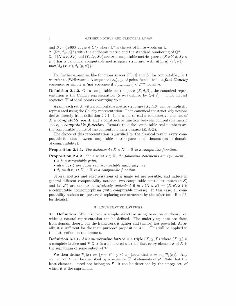
For further examples, like functions spaces C[0, 1] and Lp for computable p ≥ 1we refer to [Weihrauch]. A sequence (xn)n∈N of points is said to be a fast Cauchysequence, or simply a fast sequence if d(xn, xn+1) < 2−n for all n.

Definition 2.4.2. On a computable metric space (X, d,S), the canonical repre-sentation is the Cauchy representation (S, δC) defined by δC(−→s ) = x for all fastsequence −→s of ideal points converging to x.

Again, each set X with a computable metric structure (X, d,S) will be implicitlyrepresented using the Cauchy representation. Then canonical constructively notionsderive directly from definition 2.2.1. It is usual to call a constructive element ofX a computable point, and a constructive function between computable metricspace, a computable function. Remark that the computable real numbers arethe computable points of the computable metric space (R, d,Q).

The choice of this representation is justified by the classical result: every com-putable function between computable metric spaces is continuous (on its domainof computability).

Proposition 2.4.1. The distance d : X ×X → R is a computable function.

Proposition 2.4.2. For a point x ∈ X, the following statements are equivalent:• x is a computable point,• all d(x, si) are upper semi-computable uniformly in i,• dx := d(x, .) : X → R is a computable function.

Several metrics and effectivisations of a single set are possible, and induce ingeneral different computability notions: two computable metric structures (s,S)and (d′,S ′) are said to be effectively equivalent if id : (X, d,S) → (X, d′,S ′) isa computable homeomorphism (with computable inverse). In this case, all com-putability notions are preserved replacing one structure by the other (see [Hem02]for details).

3. Enumerative Lattices

3.1. Definition. We introduce a simple structure using basic order theory, onwhich a natural representation can be defined. The underlying ideas are thosefrom domain theory, but the framework is lighter and (hence) less powerful. Actu-ally, it is sufficient for the main purpose: proposition 3.1.1. This will be applied inthe last section on randomness.

Definition 3.1.1. An enumerative lattice is a triple (X,≤,P) where (X,≤) isa complete lattice and P ⊆ X is a numbered set such that every element x of X isthe supremum of some subset of P.

We then define P↓(x) := {p ∈ P : p ≤ x} (note that x = supP↓(x)). Anyelement of X can be described by a sequence −→p of elements of P. Note that theleast element ⊥ need not belong to P: it can be described by the empty set, ofwhich it is the supremum.


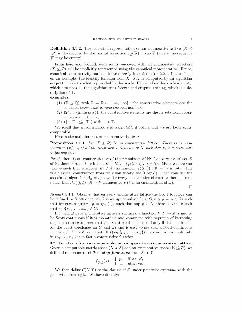
Definition 3.1.2. The canonical representation on an enumerative lattice (X,≤,P) is the induced by the partial surjection δ≤(−→p ) = sup−→p (where the sequence−→p may be empty).

From here and beyond, each set X endowed with an enumerative structure(X,≤,P) will be implicitly represented using the canonical representation. Hence,canonical constructivity notions derive directly from definition 2.2.1. Let us focuson an example: the identity function from X to X is computed by an algorithmoutputting exactly what is provided by the oracle. Hence, when the oracle is empty,which describes ⊥, the algorithm runs forever and outputs nothing, which is a de-scription of ⊥.examples:

(1) (R,≤,Q) with R = R ∪ {−∞,+∞}: the constructive elements are theso-called lower semi-computable real numbers,

(2) (2N,⊆, {finite sets}): the constructive elements are the r.e sets from classi-cal recursion theory,

(3) ({⊥,>},≤, {>}) with ⊥ < >.We recall that a real number x is computable if both x and −x are lower semi-

computable.Here is the main interest of enumerative lattices:

Proposition 3.1.1. Let (X,≤,P) be an enumerative lattice. There is an enu-meration (xi)i∈N of all the constructive elements of X such that xi is constructiveuniformly in i.

Proof. there is an enumeration ϕ of the r.e subsets of N: for every r.e subset Eof N, there is some i such that E = Ei := {ϕ(〈i, n〉) : n ∈ N}. Moreover, we cantake ϕ such that whenever Ei 6= ∅ the function ϕ(〈i, .〉) : N → N is total (thisis a classical construction from recursion theory, see [Rog87]). Then consider theassociated algorithm Aϕ = νP ◦ ϕ: for every constructive element x there is somei such that Aϕ(〈i, .〉) : N → P enumerates x (∅ is an enumeration of ⊥).

�

Remark 3.1.1. Observe that on every enumerative lattice the Scott topology canbe defined: a Scott open set O is an upper subset (x ∈ O, x ≤ y ⇒ y ∈ O) suchthat for each sequence −→p = (pni

)i∈N such that sup−→p ∈ O, there is some k suchthat sup{pn0 , . . . , pnk

} ∈ O.If Y and Z have enumerative lattice structures, a function f : Y → Z is said to

be Scott-continuous if it is monotonic and commutes with suprema of increasingsequences (one can prove that f is Scott-continuous if and only if it is continuousfor the Scott topologies on Y and Z) and is easy to see that a Scott-continuousfunction f : Y → Z such that all f(sup{pn1 , . . . , pnk

}) are constructive uniformlyin 〈n1, . . . , nk〉, is in fact a constructive function.

3.2. Functions from a computable metric space to an enumerative lattice.Given a computable metric space (X, d,S) and an enumerative space (Y,≤,P), wedefine the numbered set F of step functions from X to Y :

f〈i,j〉(x) ={pj if x ∈ Bi⊥ otherwise

We then define C(X,Y ) as the closure of F under pointwise suprema, with thepointwise ordering v. We have directly:


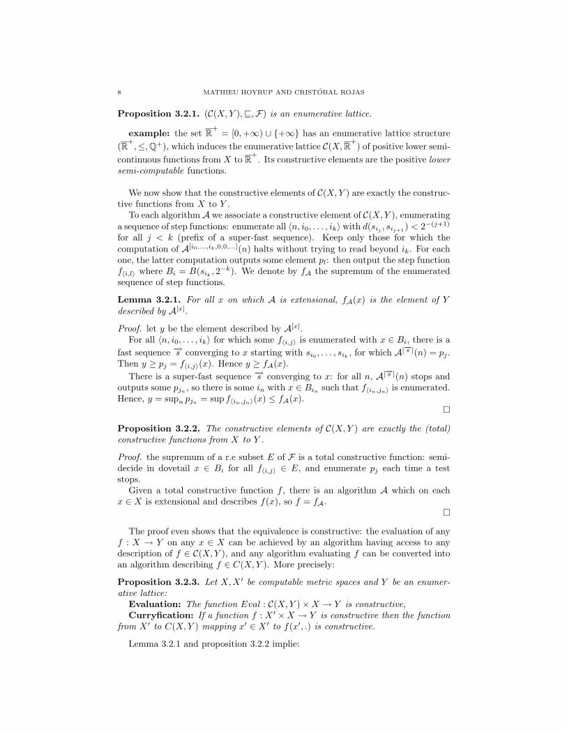
Proposition 3.2.1. (C(X,Y ),v,F) is an enumerative lattice.

example: the set R+= [0,+∞) ∪ {+∞} has an enumerative lattice structure

(R+,≤,Q+), which induces the enumerative lattice C(X,R+

) of positive lower semi-continuous functions from X to R+

. Its constructive elements are the positive lowersemi-computable functions.

We now show that the constructive elements of C(X,Y ) are exactly the construc-tive functions from X to Y .

To each algorithmA we associate a constructive element of C(X,Y ), enumeratinga sequence of step functions: enumerate all 〈n, i0, . . . , ik〉 with d(sij , sij+1) < 2−(j+1)

for all j < k (prefix of a super-fast sequence). Keep only those for which thecomputation of A[i0,...,ik,0,0,...](n) halts without trying to read beyond ik. For eachone, the latter computation outputs some element pl: then output the step functionf〈i,l〉 where Bi = B(sik , 2

−k). We denote by fA the supremum of the enumeratedsequence of step functions.

Lemma 3.2.1. For all x on which A is extensional, fA(x) is the element of Ydescribed by A[x].

Proof. let y be the element described by A[x].For all 〈n, i0, . . . , ik〉 for which some f〈i,j〉 is enumerated with x ∈ Bi, there is a

fast sequence −→s converging to x starting with si0 , . . . , sik , for which A[−→s ](n) = pj .Then y ≥ pj = f〈i,j〉(x). Hence y ≥ fA(x).

There is a super-fast sequence −→s converging to x: for all n, A[−→s ](n) stops andoutputs some pjn , so there is some in with x ∈ Bin such that f〈in,jn〉 is enumerated.Hence, y = supn pjn = sup f〈in,jn〉(x) ≤ fA(x).

�

Proposition 3.2.2. The constructive elements of C(X,Y ) are exactly the (total)constructive functions from X to Y .

Proof. the supremum of a r.e subset E of F is a total constructive function: semi-decide in dovetail x ∈ Bi for all f〈i,j〉 ∈ E, and enumerate pj each time a teststops.

Given a total constructive function f , there is an algorithm A which on eachx ∈ X is extensional and describes f(x), so f = fA.

�

The proof even shows that the equivalence is constructive: the evaluation of anyf : X → Y on any x ∈ X can be achieved by an algorithm having access to anydescription of f ∈ C(X,Y ), and any algorithm evaluating f can be converted intoan algorithm describing f ∈ C(X,Y ). More precisely:

Proposition 3.2.3. Let X,X ′ be computable metric spaces and Y be an enumer-ative lattice:

Evaluation: The function Eval : C(X,Y )×X → Y is constructive,Curryfication: If a function f : X ′ ×X → Y is constructive then the function

from X ′ to C(X,Y ) mapping x′ ∈ X ′ to f(x′, .) is constructive.

Lemma 3.2.1 and proposition 3.2.2 implie:


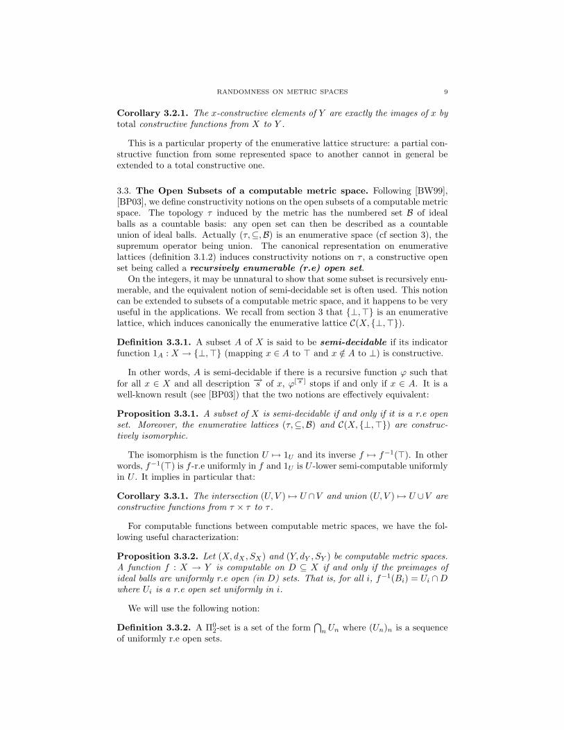
Corollary 3.2.1. The x-constructive elements of Y are exactly the images of x bytotal constructive functions from X to Y .

This is a particular property of the enumerative lattice structure: a partial con-structive function from some represented space to another cannot in general beextended to a total constructive one.

3.3. The Open Subsets of a computable metric space. Following [BW99],[BP03], we define constructivity notions on the open subsets of a computable metricspace. The topology τ induced by the metric has the numbered set B of idealballs as a countable basis: any open set can then be described as a countableunion of ideal balls. Actually (τ,⊆,B) is an enumerative space (cf section 3), thesupremum operator being union. The canonical representation on enumerativelattices (definition 3.1.2) induces constructivity notions on τ , a constructive openset being called a recursively enumerable (r.e) open set.

On the integers, it may be unnatural to show that some subset is recursively enu-merable, and the equivalent notion of semi-decidable set is often used. This notioncan be extended to subsets of a computable metric space, and it happens to be veryuseful in the applications. We recall from section 3 that {⊥,>} is an enumerativelattice, which induces canonically the enumerative lattice C(X, {⊥,>}).

Definition 3.3.1. A subset A of X is said to be semi-decidable if its indicatorfunction 1A : X → {⊥,>} (mapping x ∈ A to > and x /∈ A to ⊥) is constructive.

In other words, A is semi-decidable if there is a recursive function ϕ such thatfor all x ∈ X and all description −→s of x, ϕ[−→s ] stops if and only if x ∈ A. It is awell-known result (see [BP03]) that the two notions are effectively equivalent:

Proposition 3.3.1. A subset of X is semi-decidable if and only if it is a r.e openset. Moreover, the enumerative lattices (τ,⊆,B) and C(X, {⊥,>}) are construc-tively isomorphic.

The isomorphism is the function U 7→ 1U and its inverse f 7→ f−1(>). In otherwords, f−1(>) is f -r.e uniformly in f and 1U is U -lower semi-computable uniformlyin U . It implies in particular that:

Corollary 3.3.1. The intersection (U, V ) 7→ U ∩V and union (U, V ) 7→ U ∪V areconstructive functions from τ × τ to τ .

For computable functions between computable metric spaces, we have the fol-lowing useful characterization:

Proposition 3.3.2. Let (X, dX , SX) and (Y, dY , SY ) be computable metric spaces.A function f : X → Y is computable on D ⊆ X if and only if the preimages ofideal balls are uniformly r.e open (in D) sets. That is, for all i, f−1(Bi) = Ui ∩Dwhere Ui is a r.e open set uniformly in i.

We will use the following notion:

Definition 3.3.2. A Π02-set is a set of the form

⋂n Un where (Un)n is a sequence

of uniformly r.e open sets.


4. Computing with probability measures

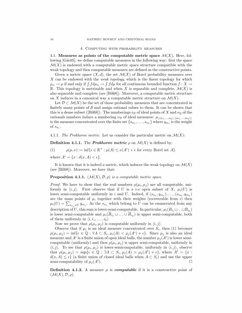
4.1. Measures as points of the computable metric space M(X). Here, fol-lowing [Gac05], we define computable measures in the following way: first the spaceM(X) is endowed with a computable metric space structure compatible with theweak topology and then computable measures are defined as the constructive points.

Given a metric space (X, d), the set M(X) of Borel probability measures overX can be endowed with the weak topology, which is the finest topology for whichµn → µ if and only if

∫fdµn →

∫fdµ for all continuous bounded function f : X →

R. This topology is metrizable and when X is separable and complete, M(X) isalso separable and complete (see [Bil68]). Moreover, a computable metric structureon X induces in a canonical way a computable metric structure on M(X).

Let D ⊂M(X) be the set of those probability measures that are concentrated infinitely many points of S and assign rational values to them. It can be shown thatthis is a dense subset ([Bil68]). The numberings νS of ideal points ofX and νQ of therationals numbers induce a numbering νD of ideal measures: µ〈〈n1,...,nk〉,〈m1,...,mk〉〉is the measure concentrated over the finite set {sn1 , . . . , snk

} where qmiis the weight

of sni.

4.1.1. The Prokhorov metric. Let us consider the particular metric on M(X):

Definition 4.1.1. The Prokhorov metric ρ on M(X) is defined by:

(1) ρ(µ, ν) := inf{ε ∈ R+ : µ(A) ≤ ν(Aε) + ε for every Borel set A}.

where Aε = {x : d(x,A) < ε}.

It is known that it is indeed a metric, which induces the weak topology on M(X)(see [Bil68]). Moreover, we have that:

Proposition 4.1.1. (M(X),D, ρ) is a computable metric space.

Proof. We have to show that the real numbers ρ(µi, µj) are all computable, uni-formly in 〈i, j〉. First observe that if U is a r.e open subset of X, µi(U) islower semi-computable uniformly in i and U . Indeed, if (sn1 , qm1), . . . , (snk

, qmk)

are the mass points of µi together with their weights (recoverable from i) thenµi(U) =

∑snj

∈U qmj . As the snj which belong to U can be enumerated from anydescription of U , this sum is lower-semi-computable. In particular, µi(Bi1∪. . .∪Bik)is lower semi-computable and µi(Bi1 ∪ . . . ∪ Bik) is upper semi-computable, bothof them uniformly in 〈i, i1, . . . , ik〉

Now we prove that ρ(µi, µj) is computable uniformly in 〈i, j〉.Observe that if µi is an ideal measure concentrated over Si, then (1) becomes

ρ(µi, µj) = inf{ε ∈ Q : ∀A ⊂ Si, µi(A) < µj(Aε) + ε}. Since µj is also an idealmeasure and Aε is a finite union of open ideal balls, the number µj(Aε) is lower semi-computable (uniformly) and then ρ(µi, µj) is upper semi-computable, uniformly in〈i, j〉. To see that ρ(µi, µj) is lower-semicomputable, uniformly in 〈i, j〉, observethat ρ(µi, µj) = sup{ε ∈ Q : ∃A ⊂ Si, µi(A) > µj(Aε) + ε}, where Aε = {x :d(x,A) ≤ ε} (a finite union of closed ideal balls when A ⊂ Si) and use the uppersemi-computability of µj(Aε). �

Definition 4.1.2. A measure µ is computable if it is a constructive point of(M(X),D, ρ).


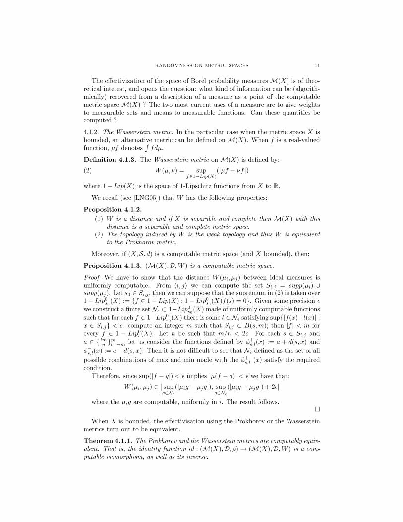
The effectivization of the space of Borel probability measures M(X) is of theo-retical interest, and opens the question: what kind of information can be (algorith-mically) recovered from a description of a measure as a point of the computablemetric space M(X) ? The two most current uses of a measure are to give weightsto measurable sets and means to measurable functions. Can these quantities becomputed ?

4.1.2. The Wasserstein metric. In the particular case when the metric space X isbounded, an alternative metric can be defined on M(X). When f is a real-valuedfunction, µf denotes

∫fdµ.

Definition 4.1.3. The Wasserstein metric on M(X) is defined by:

(2) W (µ, ν) = supf∈1−Lip(X)

(|µf − νf |)

where 1− Lip(X) is the space of 1-Lipschitz functions from X to R.

We recall (see [LNG05]) that W has the following properties:

Proposition 4.1.2.(1) W is a distance and if X is separable and complete then M(X) with this

distance is a separable and complete metric space.(2) The topology induced by W is the weak topology and thus W is equivalent

to the Prokhorov metric.

Moreover, if (X,S, d) is a computable metric space (and X bounded), then:

Proposition 4.1.3. (M(X),D,W ) is a computable metric space.

Proof. We have to show that the distance W (µi, µj) between ideal measures isuniformly computable. From 〈i, j〉 we can compute the set Si,j = supp(µi) ∪supp(µj). Let s0 ∈ Si,j , then we can suppose that the supremum in (2) is taken over1− Lip0

s0(X) := {f ∈ 1− Lip(X) : 1− Lip0s0(X)f(s) = 0}. Given some precision ε

we construct a finite set Nε ⊂ 1−Lip0s0(X) made of uniformly computable functions

such that for each f ∈ 1−Lip0s0(X) there is some l ∈ Nε satisfying sup{|f(x)−l(x)| :

x ∈ Si,j} < ε: compute an integer m such that Si,j ⊂ B(s,m); then |f | < m forevery f ∈ 1 − Lip0

s(X). Let n be such that m/n < 2ε. For each s ∈ Si,j anda ∈ { lmn }

ml=−m let us consider the functions defined by φ+

s,l(x) := a + d(s, x) andφ−s,l(x) := a− d(s, x). Then it is not difficult to see that Nε defined as the set of allpossible combinations of max and min made with the φ+−

s,l (x) satisfy the requiredcondition.

Therefore, since sup(|f − g|) < ε implies |µ(f − g)| < ε we have that:

W (µi, µj) ∈ [ supg∈Nε

(|µig − µjg|), supg∈Nε

(|µig − µjg|) + 2ε]

where the µig are computable, uniformly in i. The result follows.�

When X is bounded, the effectivisation using the Prokhorov or the Wassersteinmetrics turn out to be equivalent.

Theorem 4.1.1. The Prokhorov and the Wasserstein metrics are computably equiv-alent. That is, the identity function id : (M(X),D, ρ) → (M(X),D,W ) is a com-putable isomorphism, as well as its inverse.


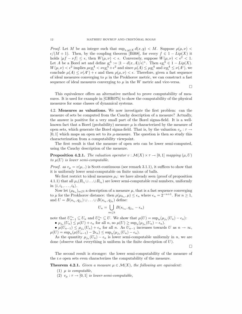
Proof. Let M be an integer such that supx,y∈X d(x, y) < M . Suppose ρ(µ, ν) <ε/(M + 1). Then, by the coupling theorem [Bil68], for every f ∈ 1 − Lip(X) itholds |µf − νf | ≤ ε, then W (µ, ν) < ε. Conversely, suppose W (µ, ν) < ε2 < 1.Let A be a Borel set and define gAε := |1 − d(x,A)/ε|+. Then εgAε ∈ 1 − Lip(X).W (µ, ν) < ε2 implies µεgAε < νεgAε +ε2 and since µ(A) ≤ µgAε and νgAε ≤ ν(Aε), weconclude µ(A) ≤ ν(Aε) + ε and then ρ(µ, ν) < ε. Therefore, given a fast sequenceof ideal measures converging to µ in the Prokhorov metric, we can construct a fastsequence of ideal measures converging to µ in the W metric and vice-versa.

�

This equivalence offers an alternative method to prove computability of mea-sures. It is used for example in [GHR07b] to show the computability of the physicalmeasures for some classes of dynamical systems.

4.2. Measures as valuations. We now investigate the first problem: can themeasure of sets be computed from the Cauchy description of a measure? Actually,the answer is positive for a very small part of the Borel sigma-field. It is a well-known fact that a Borel (probability) measure µ is characterized by the measure ofopen sets, which generate the Borel sigma-field. That is, by the valuation vµ : τ →[0, 1] which maps an open set to its µ-measure. The question is then so study thischaracterization from a computability viewpoint.

The first result is that the measure of open sets can be lower semi-computed,using the Cauchy description of the measure.

Proposition 4.2.1. The valuation operator v : M(X)× τ → [0, 1] mapping (µ,U)to µ(U) is lower semi-computable.

Proof. as vµ = v(µ, .) is Scott-continuous (see remark 3.1.1), it suffices to show thatit is uniformly lower semi-computable on finite unions of balls.

We first restrict to ideal measures µi: we have already seen (proof of proposition4.1.1) that all µi(Bi1∪. . .∪Bik) are lower semi-computable real numbers, uniformlyin 〈i, i1, . . . , ik〉.

Now let (µkn)n∈N a description of a measure µ, that is a fast sequence converging

to µ for the Prokhorov distance: then ρ(µkn , µ) ≤ εn where εn = 2−n+1. For n ≥ 1,and U = B(si1 , qj1) ∪ . . . ∪B(sik , qjk) define:

Un =⋃m≤k

B(sim , qjm − εn)

note that U εnn−1 ⊆ Un and U εnn ⊆ U . We show that µ(U) = supn(µjn(Un)− εn):• µjn(Un) ≤ µ(U) + εn for all n, so µ(U) ≥ supn(µjn(Un)− εn).• µ(Un−1) ≤ µjn(Un) + εn for all n. As Un−1 increases towards U as n → ∞,

µ(U) = supn(µ(Un−1)− 2εn) ≤ supn(µjn(Un)− εn).As the quantity µjn(Un) − εn is lower semi-computable uniformly in n, we are

done (observe that everything is uniform in the finite description of U).�

The second result is stronger: the lower semi-computability of the measure ofthe r.e open sets even characterizes the computability of the measure.

Theorem 4.2.1. Given a measure µ ∈M(X), the following are equivalent:(1) µ is computable,(2) vµ : τ → [0, 1] is lower-semi-computable,


(3) µ(Bi1 ∪ . . . ∪Bik) is lower-semi-computable uniformly in 〈i1, . . . , ik〉.

Proof. [1 ⇒ 2] Direct from proposition 4.2.1. [2 ⇒ 3] Trivial. [3 ⇒ 1] We showthat ρ(µn, µ) is upper semi-computable uniformly in n, and then use proposition2.4.2. Since ρ(µn, µ) < ε iff µn(A) < µ(Aε) + ε for all A ⊂ Sn where Sn is thefinite support of µn, and µ(Aε) is lower semi-computable (Aε is a finite union ofopen ideal balls) ρ(µn, µ) < ε is semi-decidable, uniformly in n and ε. This allowsto construct a fast sequence of ideal measures converging to µ.

�

It means that a representation which would be “tailor-made” to make the val-uation constructive, describing a measure µ by the set of integers 〈i1, . . . , ik, j〉satisfying µ(Bi1 ∪ . . .∪Bik) > qj , would be constructively equivalent to the Cauchyrepresentation. This is the approach taken in [Wei99] for the special case X = [0, 1]and in [Sch07] on an arbitrary sequential topological space. In both case, thetopology on M(X) induced by this representation is proved to be equivalent to theweak topology. A domain theoretical approach was also developed in [Eda96] on acompact space, the Scott topology being proved to induce the weak topology.

4.2.1. The examples of the Cantor space and the unit interval. On the Cantor spaceΣN (where Σ is a finite alphabet) with its natural computable metric space struc-ture, the ideal balls are the cylinders. As a finite union of cylinders can alwaysbe expressed as a disjoint (and finite) union of cylinders, and the complement of acylinder is a finite union of cylinders, we have:

Corollary 4.2.1. A measure µ ∈ M(ΣN) is computable iff the measures of thecylinders are uniformly computable.

On the unit real interval, ideals balls are open rational intervals. Again, a finiteunion of such intervals can always be expressed as a disjoint (and finite) union ofopen rational intervals. Then:

Corollary 4.2.2. A measure µ ∈ M([0, 1]) is computable iff the measures of therational open intervals are uniformly lower-semi-computable.

If µ has no atoms, a rational open interval is the complement of at most twodisjoint open rational intervals, up to a null set. In this case, µ is then computableiff the measures of the rational intervals are uniformly computable.

4.3. Measures as integrals. We now answer the second question: is the integralof functions computable from the description of a measure ?

The computable metric space structure of X and the enumerative lattice struc-ture of R+

induce in a canonical way the enumerative space C(X,R+) (see section

3.2), which is actually the set of lower semi-continuous functions from X to R+.

We have:

Proposition 4.3.1. The integral operator∫

: M(X) × C(X,R+) → R+

is lowersemi-computable.


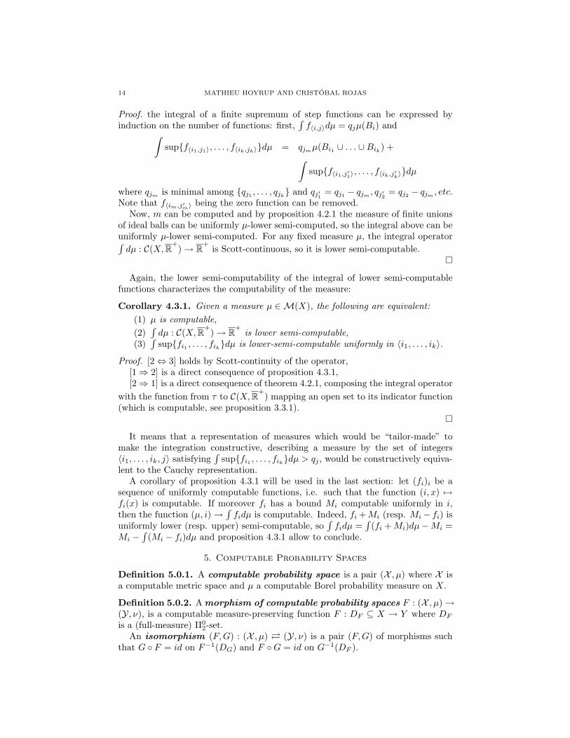
Proof. the integral of a finite supremum of step functions can be expressed byinduction on the number of functions: first,

∫f〈i,j〉dµ = qjµ(Bi) and∫

sup{f〈i1,j1〉, . . . , f〈ik,jk〉}dµ = qjmµ(Bi1 ∪ . . . ∪Bik) +∫sup{f〈i1,j′1〉, . . . , f〈ik,j′k〉}dµ

where qjm is minimal among {qj1 , . . . , qjk} and qj′1 = qj1 − qjm , qj′2 = qj2 − qjm , etc.Note that f〈im,j′m〉 being the zero function can be removed.

Now, m can be computed and by proposition 4.2.1 the measure of finite unionsof ideal balls can be uniformly µ-lower semi-computed, so the integral above can beuniformly µ-lower semi-computed. For any fixed measure µ, the integral operator∫dµ : C(X,R+

) → R+is Scott-continuous, so it is lower semi-computable.

�

Again, the lower semi-computability of the integral of lower semi-computablefunctions characterizes the computability of the measure:

Corollary 4.3.1. Given a measure µ ∈M(X), the following are equivalent:(1) µ is computable,(2)

∫dµ : C(X,R+

) → R+is lower semi-computable,

(3)∫

sup{fi1 , . . . , fik}dµ is lower-semi-computable uniformly in 〈i1, . . . , ik〉.

Proof. [2 ⇔ 3] holds by Scott-continuity of the operator,[1 ⇒ 2] is a direct consequence of proposition 4.3.1,[2 ⇒ 1] is a direct consequence of theorem 4.2.1, composing the integral operator

with the function from τ to C(X,R+) mapping an open set to its indicator function

(which is computable, see proposition 3.3.1).�

It means that a representation of measures which would be “tailor-made” tomake the integration constructive, describing a measure by the set of integers〈i1, . . . , ik, j〉 satisfying

∫sup{fi1 , . . . , fik}dµ > qj , would be constructively equiva-

lent to the Cauchy representation.A corollary of proposition 4.3.1 will be used in the last section: let (fi)i be a

sequence of uniformly computable functions, i.e. such that the function (i, x) 7→fi(x) is computable. If moreover fi has a bound Mi computable uniformly in i,then the function (µ, i) →

∫fidµ is computable. Indeed, fi +Mi (resp. Mi− fi) is

uniformly lower (resp. upper) semi-computable, so∫fidµ =

∫(fi +Mi)dµ−Mi =

Mi −∫

(Mi − fi)dµ and proposition 4.3.1 allow to conclude.

5. Computable Probability Spaces

Definition 5.0.1. A computable probability space is a pair (X , µ) where X isa computable metric space and µ a computable Borel probability measure on X.

Definition 5.0.2. A morphism of computable probability spaces F : (X , µ) →(Y, ν), is a computable measure-preserving function F : DF ⊆ X → Y where DF

is a (full-measure) Π02-set.

An isomorphism (F,G) : (X , µ) � (Y, ν) is a pair (F,G) of morphisms suchthat G ◦ F = id on F−1(DG) and F ◦G = id on G−1(DF ).


We recall that F is measure-preserving if ν(A) = µ(F−1(A)) for all Borel set A.

5.1. Generalized binary representations. The Cantor space 2ω (2 denotes{0, 1}) is a privileged place for computability. This can be understood by thefact that it is the countable product (with the product topology) of a finite space(with the discrete topology). A consequence of this is that membership of a basicopen set (cylinder) boils down to a pattern-matching and is then decidable. Asdecidable sets must be clopen, this property cannot hold in connected spaces. Asa result, a computable metric space is not in general constructively homeomorphicto the Cantor space.

Nevertheless, the real unit interval [0, 1] is not so far away from the Cantor space.The binary numeral system provides a correspondence between real numbers andbinary sequences, which is certainly not homeomorphic, unless we remove the smallset of dyadic numbers. In particular, the remaining set is totally disconnected, andthe dyadic intervals form a basis of clopen sets.

Actually, this correspondence makes the computable probability space [0, 1] withthe Lebesgue measure isomorphic to the Cantor space with the uniform measure.This fact has been implicitly used, for instance, to extend algorithmic randomnesson the Cantor space with the uniform measure to the unit interval with the Lebesguemeasure.

We extend this to any computable probability space defining the notion of binaryrepresentation, and show that every computable probability space has a binary rep-resentation, which implies in particular that every computable probability space isisomorphic to the Cantor space with a computable measure. To carry out this gen-eralization, let us briefly scrutinize the binary numeral system on the unit interval:δ : 2ω → [0, 1] is a total surjective morphism. Every non-dyadic real has a unique

expansion, and the inverse of δ, defined on the set D of non-dyadic numbers, iscomputable. Moreover, D is large both in a topological and measure-theoreticalsense: it is a residual (a countable intersection of dense open sets) and has measureone. (δ, δ−1) is then an isomorphism.

In our generalization, we do not require every binary sequence to be the expan-sion of a point, which would force X to be compact.

Definition 5.1.1. A binary representation of a computable probability space(X , µ) is a pair (δ, µδ) where µδ is a computable probability measure on 2ω andδ : (2ω, µδ) → (X , µ) is a surjective morphism such that, calling δ−1(x) the set ofexpansions of x ∈ X:• there is a dense full-measure Π0

2-set D of points having a unique expansion,• δ−1 : D → δ−1(D) is computable.

Remark that when the support of the measure (the smallest closed set of fullmeasure) is the whole space X, like the Lebesgue measure on the interval, a full-measure Π0

2-set is always a residual, but in general it is only dense on the supportof the measure: that is the reason why we explicitly require D to be dense. Alsoremark that a binary representation δ always induces an isomorphism (δ, δ−1) be-tween the Cantor space and the computable probability space.

The sequel of this section is devoted to the proof of the following result:

Theorem 5.1.1. Every computable probability space (X , µ) has a binary represen-tation.


The space, restricted to the domain D of the isomorphism, is then totally dis-connected: the preimages of the cylinders form a basis of clopen and even decidablesets. In the whole space, they are not decidable any more. Instead, they are almostdecidable.

Definition 5.1.2. A set A is said to be almost decidable if there are two r.eopen sets U and V such that:

U ⊂ A, V ⊆ AC , U ∪ V is dense and has measure one

Definition 5.1.3. A measurable setA is said to be µ-continuous or a µ-continuityset if µ(∂A) = 0 where ∂A = A ∩X \A is the boundary of A.

Remark that, as for subsets of N, a set is almost decidable if and only if itscomplement is a.s. decidable. An almost decidable set is always a continuity set.Let B(s, r) be a µ-continuous ball with computable radius: in general it is notan almost decidable set (for instance, isolated points may be at distance exactly rfrom s). But if there is no ideal point is at distance r from s, then B(s, r) is almostdecidable: take U = B(s, r) and V = X \B(s, r).

We say that the elements of a sequence (Ai)i∈N are uniformly a.s. decidableif there are two sequences (Ui)i∈N and (Vi)i∈N of uniformly r.e sets satisfying theconditions above.

Lemma 5.1.1. There is a sequence (rn)n∈N of uniformly computable reals suchthat (B(si, rn))〈i,n〉 is a basis of uniformly almost decidable balls.

Proof. define U〈i,k〉 = {r ∈ R+ : µ(B(si, r)) < µ(B(si, r))+1/k}: by computabilityof µ, this is a r.e open subset of R+, uniformly in 〈i, k〉. It is furthermore dense inR+: the spheres Sr = B(si, r) \B(si, r) form a partition of the space when r variesin R+ and µ is finite, so the set of r for which µ(Sr) ≥ 1/k is finite.

Define V〈i,j〉 = R+ \ {d(si, sj)}: this is a dense r.e open set, uniformly in 〈i, j〉.Then by the computable Baire Category Theorem (see [YMT99], [Bra01]), the

dense Π02-set

⋂〈i,k〉 U〈i,k〉 ∩

⋂〈i,j〉 V〈i,j〉 contains a sequence (rn)n∈N of uniformly

computable real numbers which is dense in R+. In other words, all rn are com-putable, uniformly in n. By construction, for any si and rn, B(si, rn) is almostdecidable.

We recall that from an enumeration (In)n∈N of all the rational compact intervalsof R+, rn is constructed computing a nested shrinking sequence (Jnk )k∈N of rationalcompact intervals starting from Jn0 = In, and such that Jnk+1 ⊆ Jnk ∩Uk ∩Vk. Then{rn} =

⋂k J

nk .

�

We will denote B(si, rn) by Bµk where k = 〈i, n〉. Note that different algorithmicdescriptions of the same µmay yield different sequences (rn)n∈N, so Bµk is an abusivenotation. It is understood that some algorithmic description of µ has been chosenand fixed. This can be done only because the measure µ is computable, which isthen a crucial hypothesis. We denote X \B(si, rn) by Cµk and define:

Definition 5.1.4. For w ∈ 2∗, the cell Γ(w) is defined by induction on |w|:

Γ(ε) = X, Γ(w0) = Γ(w) ∩ Cµi and Γ(w1) = Γ(w) ∩Bµiwhere ε is the empty word and i = |w|.


This an almost decidable set, uniformly in w.

Proof. (of theorem 5.1.1). We construct an encoding function b : D → 2ω, adecoding function δ : Dδ → X, and show that δ is a binary representation, withb = δ−1.

Encoding.Let D =

⋂iB

µi ∪C

µi : this is a dense full-measure Π0

2-set. Define the computablefunction b : D → 2ω by:

b(x)i ={

1 if x ∈ Bµi0 if x ∈ Cµi

Let x ∈ D: ω = b(x) is also characterized by {x} =⋂i Γ(ω0..i−1). Let µδ be

the image measure of µ by b: µδ = µ ◦ b−1. b is then a morphism from (X,µ) to(2ω, µδ).

Decoding.Let Dδ be the set of binary sequences ω such that

⋂i Γ(ω0..i−1) is a singleton.

We define the decoding function δ : Dδ → X by:

δ(ω) = x if⋂i

Γ(ω0..i−1) = {x}

ω is called an expansion of x. Remark that x ∈ Bµi ⇒ ωi = 1 and x ∈ Cµi ⇒ωi = 0, which implies in particular that if x ∈ D, x has a unique expansion, whichis b(x). Hence, b = δ−1 : δ−1(D) → D and µδ(Dδ) = µ(D) = 1.

We now show that δ : Dδ → X is a surjective morphism. For seek of clarity, thecenter and the radius of the ball Bµi will be denoted si and ri respectively. Let uscall i an n-witness for ω if ri < 2−(n+1), ωi = 1 and Γ(ω0..i) 6= ∅.• Dδ is a Π0

2-set: we show that Dδ =⋂n{ω ∈ 2ω : ω has a n-witness}.

Let ω ∈ Dδ and x = δ(ω). For each n, x ∈ B(si, ri) for some i with ri < 2−(n+1).Since x ∈ Γ(ω0..i), we have that Γ(ω0..i) 6= ∅ and ωi = 1 (otherwise Γ(ω0..i) isdisjoint of Bµi ). In other words, i is an n-witness for ω.

Conversely, if ω has a n-witness in for all n, since Γ(ω0..in) ⊆ Bµin whose radiustends to zero, the nested sequence (Γ(ω0..in))n of closed cells has, by completenessof the space, a non-empty intersection, which is a singleton.• δ : Dδ → X is computable. For each n, find some n-witness in of ω: the

sequence (sin)n is a fast sequence converging to δ(ω).• δ is surjective: we show that each point x ∈ X has at least one expansion.

To do this, we construct by induction a sequence ω = ω0ω1 . . . such that for all i,x ∈ Γ(ω0 . . . ωi). Let i ≥ 0 and suppose that ω0 . . . ωi−1 (empty when i = 0) hasbeen constructed. As Bµi ∪ C

µi is open dense and Γ(ω0..i−1) is open, Γ(ω0..i−1) =

Γ(ω0..i−1) ∩ (Bµi ∪ Cµi ) which equals Γ(ω0..i−10) ∪ Γ(ω0..i−11). Hence, one choice

for ωi ∈ {0, 1} gives x ∈ Γ(ω0..i).By construction, x ∈

⋂i Γ(ω0..i−1). As (Bµi )i is a basis and ωi = 1 whenever

x ∈ Bµi , ω is an expansion of x.�

5.2. Another characterization of the computability of measures. The ex-istence of a basis of almost decidable sets also leads to another characterization ofthe computability of measures, which is reminiscent of what happens on the Cantorspace (see corollary 4.2.1). Let us say that two bases (Ui)i and (Vi)i of the topology


τ are constructively equivalent if both idτ : (τ,⊆,U) → (τ,⊆,V) and its inverse areconstructive functions between enumerative lattices.

Corollary 5.2.1. A measure µ ∈ M(X) is computable if and only if there is abasis U = (Ui)i∈N of uniformly almost decidable open sets which is constructivelyequivalent to B and such that all µ(Ui1 ∪ . . . ∪ Uik) are computable uniformly in〈i1, . . . , ik〉.

Proof. if µ is computable, the a.s. decidable balls U〈i,n〉 = B(si, rn) are basiswhich is constructively equivalent to B: indeed, B(si, rn) =

⋃qj<rn

B(si, qj) andB(si, qj) =

⋃rn<qj

B(si, rn), and rn is computable uniformly in n.For the converse, the valuation function fµ is lower semi-computable. Indeed,

the r.e open sets are uniformly r.e relatively to the basis U , so their measures canbe lower-semi-computed, computing the measures of finite unions of elements of U .Hence µ is computable by theorem 4.2.1.

�

6. Algorithmic randomness

On the Cantor space with a computable measure µ, Martin-Lof originally definedthe notion of an individual random sequence as a sequence passing all µ-randomnesstests. A µ-randomness test a la Martin-Lof is a sequence of uniformly r.e open sets(Un)n satisfying µ(Un) ≤ 2−n. The set

⋂n Un has null measure, in an effective way:

it is then called an effective null set.Equivalently, a µ-randomness test can be defined as a positive lower semi-

computable function t : 2ω → R satisfying∫tdµ ≤ 1 (see [VV93] for instance).

The associated effective null set is {x : t(x) = +∞} =⋂n{x : t(x) > 2n}. Actually,

every effective null set can be put in this form for some t. A point is then calledµ-random if it lies in no effective null set.

Following Gacs, we will use the second presentation of randomness tests whichis more suitable to express uniformity.

6.1. Randomness w.r.t any probability measure.

Definition 6.1.1. Given a measure µ ∈ M(X), a µ-randomness test is a µ-constructive element t of C(X,R+

), such that∫tdµ ≤ 1. Any subset of {x ∈ X :

t(x) = +∞} is called a µ-effective null set.A uniform randomness test is a constructive function T from M(X) to

C(X,R+) such that for all µ ∈M(x),

∫Tµdµ ≤ 1 where Tµ denotes T (µ).

Note that T can be also seen as a lower-semi-computable function from M(X)×X to R+

(see section 3.2).A presentation a la Martin-Lof can be directly obtained using the functions

below:

F : C(X,R+) → τN

t 7→ (t−1(2n,+∞))nG : τN → C(X,R+

)(Un)n 7→ (x 7→ sup{n : x ∈

⋂i≤n Ui})

which are constructive, satisfy F ◦G = id : τN → τN and preserve the correspondingeffective null sets.


A uniform randomness test T induces a µ-randomness test Tµ for all µ. Weshow two important results which hold on any computable metric space:• the two notions are actually equivalent (theorem 6.1.1),• there is a universal uniform randomness test (theorem 6.1.2).The second result was already obtained by Gacs, but only on spaces which have

recognizable Boolean inclusions, which is an additional computability property onthe basis of ideal balls.

By proposition 3.2.2, constructive functions from M(X) to C(X,R+) can be

identified to constructive elements of the enumerative lattice C(M(X), C(X,R+)).

Let (Hi)i∈N be an enumeration of all its constructive elements (proposition 3.1.1):Hi = supk fϕ(i,k) where ϕ : N2 → N is some recursive function and the fn are stepfunctions.

Lemma 6.1.1. There is a constructive function T : N×M(X) → C(X,R+) satis-

fying:• for all i, Ti = T (i, .) is a uniform randomness test,• if

∫Hi(µ)dµ < 1 for some µ, then Ti(µ) = Hi(µ).

Proof. To enumerate only tests, we would like to be able to semi-decide∫

supk<n fϕ(i,k)(µ)dµ <1. But supk<n fϕ(i,k)(µ) is only lower semi-computable (from µ). To overcome thisproblem, we use another class of basic function.

Let Y be a computable metric space: for an ideal point s of Y and positiverationals q, r, ε, define the hat function:

hq,s,r,ε(y) := q.[1− [d(y, s)− r]+/ε]+

where [a]+ = max{0, a}. This is a continuous function whose value is q in B(s, r),0 outside B(s, r + ε). The numberings of S and Q>0 induce a numbering (hn)n∈Nof all the hat functions. They can be taken as an alternative to step functionsin the enumerative lattice C(Y,R+

): they yield the same computable structure.Indeed, step functions can be constructively expressed as suprema of such functions:f〈i,j〉 = sup{hqj ,s,r−ε,ε : 0 < ε < r} where Bi = B(s, r), and conversely.

We apply this to Y = M(X)×X endowed with the canonical computable metricstructure. By Curryfication it provides functions hn ∈ C(M(X), C(X,R+

)) withwhich the Hi can be expressed: there is a recursive function ψ : N2 → N such thatfor all i, Hi = supk hψ(i,k).

Furthermore, hn(µ) (strictly speaking, Eval(hn, µ), see proposition 3.2.3) isbounded by a constant computable from n and independent of µ. Hence, the inte-gration operator

∫: M(X)×N → [0, 1] which maps (µ, 〈i1, . . . , ik〉) to

∫sup{hi1(µ), . . . , hik(µ)}dµ

is computable.We are now able to define T : T (i, µ) = sup{Hk

i (µ) :∫Hki (µ)dµ < 1} where

Hki = supn<k hψ(i,n). As

∫Hki (µ)dµ can be computed from i, k and a description

of µ, T is a constructive function from N×M(X) to C(X,R+).

�

As a consequence, every randomness test for a particular measure can be ex-tended to a uniform test:

Theorem 6.1.1 (Uniformity vs non-uniformity). Let µ0 be a measure. For everyµ0-randomness test t there is a uniform randomness test T : M(X) → C(X,R+

)with T (µ0) = 1

2 t.


Proof. let µ0 be a measure and t a µ0-randomness test: 12 t is then a µ0-constructive

element of the enumerative lattice C(X,R+), so by lemma 3.2.1 there is a construc-

tive element H of C(M(X), C(X,R+)) such that H(µ0) = 1

2 t. There is some isuch that H = Hi: Ti is a uniform randomness test satisfying Ti(µ0) = 1

2 t because∫Hi(µ0)dµ0 = 1

2

∫tdµ0 < 1.

�

Theorem 6.1.2 (Universal uniform test). There is a universal uniform randomnesstest, that is a uniform test Tu such that for every uniform test T there is a constantcT with Tu ≥ cTT .

Proof. it is defined by Tu :=∑i 2

−i−1Ti: as every Ti is a uniform randomness test,Tu is also a uniform randomness test, and if T is a uniform impossibility test, thenin particular 1

2T is a constructive element of C(M(X), C(X,R+)), so 1

2T = Hi forsome i. As

∫Hi(µ)dµ = 1

2

∫T (µ)dµ < 1 for all µ, Ti(µ) = Hi(µ) = 1

2T (µ) for allµ, that is Ti = 1

2T . So Tu ≥ 2−i−2T .�

Definition 6.1.2. Given a measure µ, a point x ∈ X is called µ-random ifTµu (x) <∞. Equivalently, x is µ-random if it lies in no µ-effective null set.

The set of µ-random points is denoted by Rµ. This is the complement of themaximal µ-effective null set {x ∈ X : Tµu (x) = +∞}.

6.2. Randomness on a computable probability space. We study the particu-lar case of a computable measure. As a morphism of computable probability spacesis compatible with measures and computability structures, it shall be compatiblewith algorithmic randomness. Indeed:

Proposition 6.2.1. Morphisms of computable probability spaces are defined onrandom points and preserve randomness.

To prove it, we shall use the following lemma:

Lemma 6.2.1. In a computable probability space (X , µ), every random point liesin every r.e open set of full measure.

Proof. let U =⋃〈i,j〉∈E B(si, qj) be a r.e open set of measure one, with E a r.e

subset of N. Let F be the r.e set {〈i, k〉 : ∃j, 〈i, j〉 ∈ E, qk < qj}. Define:

Un =⋃

〈i,k〉∈F∩[0,n]

B(si, qk) and V Cn =

⋃〈i,k〉∈F∩[0,n]

B(si, qk)

Then Un and Vn are r.e uniformly in n, Un ↗ U and UC =⋂n Vn. As µ(Un) is

lower semi-computable uniformly in n, a sequence (ni)i∈N can be computed suchthat µ(Uni

) > 1 − 2−i. Then µ(Vni) < 2−i, and UC =

⋂i Vni

is a µ-Martin-Loftest. Therefore, every µ-random point is in U .

�

Proof. (of proposition 6.2.1) let F : D ⊆ X → Y be a morphism. From lemma6.2.1, every random point is in D which is an intersection of full-measure r.e opensets.

Let t : Y → R+be the universal ν-test. The function t ◦ F : D → R+

is lowersemi-computable. Let A be any algorithm lower semi-computing it: the associated


lower semi-computable function fA : X → R+extends t ◦ F to the whole space X

(see lemma 3.2.1). As µ(D) = 1,∫t ◦ Fdµ is well defined and equals

∫fAdµ. As

F is measure-preserving,∫t ◦ Fdµ =

∫tdν ≤ 1. Hence fA is a µ-test. Let x ∈ X

be a µ-random point: as x ∈ D, t(F (x)) = fA(x) < +∞, so F (x) is ν-random.�

Corollary 6.2.1. Let (F,G) : (X , µ) � (Y, ν) be an isomorphism of computableprobability spaces. Then F|Rµ

and G|Rνare total computable bijections between Rµ

and Rν , and (F|Rµ)−1 = G|Rν

.

In particular:

Corollary 6.2.2. Let δ be a binary representation on a computable probability space(X , µ). Each point having a µδ-random expansion is µ-random and each µ-randompoint has a unique expansion, which is µδ-random.

This proves that algorithmic randomness over a computable probability spacecould have been defined encoding points into binary sequences using a binary rep-resentation: this would have led to the same notion of randomness. Using thisprinciple, a notion of Kolmogorov complexity characterizing Martin-Lof random-ness comes for free. For x ∈ D, define:

Hn(x) = H(ω0..n−1) and Γn(x) = δ([ω0..n−1])

where ω is the expansion of x and H is the prefix Kolmogorov complexity.

Corollary 6.2.3. Let δ be a binary representation on a computable probabilityspace (X , µ). Then x is µ-random if and only if there is c such that for all n:

Hn(x) ≥ − logµ(Γn(x))− c

All this allows to treat algorithmic randomness within probability theory overgeneral metric spaces. In [GHR07a] for instance, it is applied to show that in ergodicsystems over metric spaces, algorithmically random points are well-behaved: theyare typical with respect to any computable measure preserving transformation,generalizing what has been proved in [V’y97] for the Cantor space.

Aknowledgments

We would like to thank Stefano Galatolo, Peter Gacs and Giuseppe Longo foruseful comments and remarks.

References

[AJ94] Samson Abramsky and Achim Jung. Domain theory. In S. Abramsky, D. Gabbay, andT. S. E. Maibaum, editors, Handbook of Logic in Computer Science Volume 3, pages

1–168. Oxford University Press, 1994.[Bil68] Patrick Billingsley. Convergence of Probability Measures. John Wiley, New York, 1968.[BP03] Vasco Brattka and Gero Presser. Computability on subsets of metric spaces. Theoretical

Computer Science, 305(1-3):43–76, 2003.

[Bra01] Vasco Brattka. Computable versions of baire’s category theorem. In MFCS ’01: Pro-ceedings of the 26th International Symposium on Mathematical Foundations of Com-puter Science, pages 224–235, London, UK, 2001. Springer-Verlag.

[BW99] Vasco Brattka and Klaus Weihrauch. Computability on subsets of euclidean space i:Closed and compact subsets. Theoretical Computer Science, 219(1-2):65–93, 1999.


[Eda96] Abbas Edalat. The Scott topology induces the weak topology. In LICS ’96: Proceed-

ings of the 11th Annual IEEE Symposium on Logic in Computer Science, page 372,

Washington, DC, USA, 1996. IEEE Computer Society.[Gac05] Peter Gacs. Uniform test of algorithmic randomness over a general space. Theoretical

Computer Science, 341:91–137, 2005.

[GHR07a] Stefano Galatolo, Mathieu Hoyrup, and Cristobal Rojas. Algorithmically randompoints in measure preserving systems, statistical behaviour, complexity and entropy.

Submitted to Information and Computation, 2007. Available on arxiv.

[GHR07b] Stefano Galatolo, Mathieu Hoyrup, and Cristobal Rojas. An effective Borel-Cantellilemma. Constructing orbits with required statistical properties. Submitted to JEMS,

2007. Available on arxiv.

[Hem02] Armin Hemmerling. Effective metric spaces and representations of the reals. Theor.Comput. Sci., 284(2):347–372, 2002.

[HW98] Peter Hertling and Klaus Weihrauch. Randomness spaces. In Kim G. Larsen, SvenSkyum, and Glynn Winskel, editors, Automata, Languages and Programming, volume

1443 of Lecture Notes in Computer Science, pages 796–807, Berlin, 1998. Springer.

25th International Colloquium, ICALP’98, Aalborg, Denmark, July 1998.[HW03] Peter Hertling and Klaus Weihrauch. Random elements in effective topological spaces

with measure. Information and Computation, 181(1):32–56, 2003.

[KF82] Ker-I Ko and H. Friedman. Computational complexity of real functions. TheoreticalComputer Science, 20(3):323–352, 1982.

[Ko91] Ker-I Ko. Complexity Theory of Real Functions. Birkhauser Boston Inc., Cambridge,

MA, USA, 1991.[LNG05] Ambrosio L, Gigli N, and Savare G. Gradient flows: in metric spaces and in the space

of probability measures. Birkhauser, Zurich, 2005.

[ML66] Per Martin-Lof. The definition of random sequences. Information and Control,9(6):602–619, 1966.

[Rog87] Hartley Jr. Rogers. Theory of Recursive Functions and Effective Computability. MITPress, Cambridge, MA, USA, 1987.

[Sch07] Matthias Schroder. Admissible representations of probability measures. Electronic

Notes in Theoretical Computer Science, 167:61–78, 2007.[VV93] Vladimir G. Vovk and Vladimir V. Vyugin. On the empirical validity of the bayesian

method. Journal of the Royal Statistical Society, B 55(1):253–266, 1993.

[V’y97] Vladimir V. V’yugin. Effective convergence in probability and an ergodic theoremfor individual random sequences. SIAM Theory of Probability and Its Applications,

42(1):39–50, 1997.

[Wei99] Klaus Weihrauch. Computability on the probability measures on the borel sets of theunit interval. Theoretical Computer Science, 219:421–437, 1999.

[Wei00] Klaus Weihrauch. Computable Analysis. Springer, Berlin, 2000.

[YMT99] Mariko Yasugi, Takakazu Mori, and Yoshiki Tsujii. Effective properties of sets andfunctions in metric spaces with computability structure. Theoretical Computer Science,

219(1-2):467–486, 1999.

LIENS, Ecole Normale Superieure, Paris. email: [email protected]

LIENS, Ecole Normale Superieure and CREA, Ecole Polytechnique, Paris. email:

[email protected]

Computability of probability measures and Martin-Lof randomness over metric spaces

Documents

Transcript of Computability of probability measures and Martin-Lof randomness over metric spaces