Using surface-syntactic parser and Derivation fromRandomness

X-IOTA IR system used for CLIPS Mono &Bilingual Experiments for CLEF 2004

Gilles SerassetLaboratoire CLIPS-IMAG∗

Grenoble FranceGilles.Serasset@imag.fr

Jean-Pierre ChevalletIPAL-CNRS, I2R A*STAR

National University of Singaporeviscjp@i2r.a-star.edu.sg

Abstract

This document present work we have done for the CLEF 2004 participation. We promotethe use of surface-syntactic parsing to extract indexing terms. We also promote the DerivationFrom Randomness weighting. For the bilingual part, we have tested reinforcement queryweighting using an association thesaurus.

1 IntroductionIn our previous participation at CLEF in 2003 [3], we have tested the use of an associationthesaurus to enhance query translation. We have only use the association thesaurus to add somenew terms to the proposed translation terms. In our current participation, we have tried anotheruse of such a thesaurus: we do not enlarge the query, but rather we use it to modify the weighingof a given translated query. Our basic idea is the selection of the best term translation usingquery context and association thesaurus from the corpus. Last year, we have neglected the studyof the matching function and the influence of the weighting scheme. For this participation we willalso focus on this aspect: we have test the Derivation From Randomness (DFR) against Okapimeasure and some other classical IR weighting. We also promote the use of a surface-syntacticparser. All documents are first transform by the parser. The stemming is then proposed by theparser. Finnish is an agglutinative language, and using such an NL parsing enable to correctlysplit the glued words into separated correct indexing terms.

The paper present first the training experiments performed on 2003 collection in part 2. Inpart 3 we discuss the monolingual results. Then, in part 4, we present the technique used forbilingual results and present hypothesis based on the results.

2 Training on monolingual runIn this part, we present some training we have achieved using monolingual corpus of CLEF 2003.We have mainly used the Finnish and French corpus. The purpose of this training is to select thebest weighting scheme for the given CLEF document collection.

∗This work is part of the PRISM-IMAG project devoted to high level indexing representation using interlingualgraph formalism.

1

2.1 The underlying IR modelAll experiments are grounded on the classic vector space model. Goal of experiment is to comparethe probabilistic model of Okapi with Derivation From Randomness model, versus more classicalweightings. This comparison will be done on two different languages.

Basically, the final matching process is achieved by a product between query vector and docu-ment matrix, which computes the Relevant Status Value (RSV) of all document against the query.For a query vector Q = (qi) with a dimension of t term i ∈ [1..t], and a index document matrix ofn documents Dj = (dij), j ∈ [1..n], the RSV is computed by:

RSV (Q, Dj) =∑

i∈[1..t]

qi ∗ dij

We keep this matching process for all tests, the changes are in the documents and query processingto select indexing terms, and in the weighting scheme. We recall here the scheme that is inspired bythe SMART system. We suppose the previous processing steps have produced a matrix D = (di,j).Usually, the value di,j is only the result of term ti counting in the document Dj, called termfrequency tfij . Each weighting scheme can be decomposed in three steps: a local, a global and anormalization step. The local is related to only one vector. All these transformations are listed intable 1. For all measure we use the following symbols:

fi total number of term i in the corpusd∗ij is a normalization of dij

λi is the fraction fi

TT is the corpus size : T =

∑i fi

dfi the document frequency of idij current value in the matrixc a constant for DFRL(Dj) the length of Dj equals to

∑t dij

awr(L(Dj)) mean document length equals to∑

jL(Dj)

nn number of document in the corpust number of unique terms in the corpusqi weight of term i of query q

n wij = dij none, no changeb wij = 1 binarya wij = 0.5+0.5∗dij

maxi(dij)local max

l wij = ln(dij + 1) natural logd wij = ln(ln(dij + 1) + 1) double natural log

Table 1: Local weighting

The global weighting is related to the matrix, and then it is a weighing which takes into accountthe relative importance of a term regarding the whole document collection. The most famous isthe Inverse Document Frequency : Idf. The table 2 lists the global weighting we have tested.Okapi and DFR are not global weighting per se but rather complete weighting scheme themselves.In our X-IOTA system, they are computed at the same time than global weighting, and it istechnically feasible to use them with a local and a final normalization. DFR is presented in thenext part.

The Okapi measure described in [5, 4], uses the length of the document, the function L(),and also a normalization by the average length of all documents in the corpus, the function A().This length is related to the number of indexing terms in a document. The Okapi measure uses2 constants values called k1 and b. Finally, the last treatment is the normalization of the finalvector.

n wij = dij none, no global changet wij = dij ∗ log n

dfiIdf

p wij = dij ∗ log n−dfi

dfiIdf variant for Okapi

O wij = (k1+1)∗dij

k1∗[(1−b)+b∗ L(dj)A(dj) ]+dij

Okapi

R (see below) DFR

Table 2: Global weighting

n wij = dij none, no normalizationc wij = dij√∑

id2

ij

cosine

Table 3: Final normalization

A weighting scheme is composed by the combination of the local, global and final weighting.We represent a weighting scheme by 3 letters. For example, nnn is only the raw term frequency.The scheme bnn for both documents and queries leads to a sort of Boolean model where everyterm in the query is considered connected by a conjunction. In that case the RVS counts the termsintersection between documents and queries. The c normalization applied to both document andquery vector leads to the computation of the cosine between these two vectors. This is the classicalvector space model if we use the ltc scheme for document and queries. The scheme nOn for thedocuments, and npn with the queries, is the Okapi model, and the use of nRn for document andnnn for the queries is the DFR model. For these two models, constants have to be defined.

Notice that the c normalization of the queries, leads to divide the RSV for this query by√∑i q2

i . For each query this is a constant value which does not influence the relative order ofanswered document list. It follows that this normalization is useless for queries and should not beused. In the next section we briefly present the derivation from Randomness weighting that seemsto give best results, and that we have used for all CLEF 2004 runs.

2.2 derivation from randomness (DFR)This weighting scheme has been proposed by Gianni Amati in [1] (with a small error in thedefinition of the value f∗

t,d). Theoretical discussions about this approach can be found in [2].Figure 4 sum up the results we obtain using this weighting scheme, on the CLEF2003 queries fortraining using the formula described in [1]. The formula is given by:

wij = (log2(1 + λi) + d∗ij ∗ log2

1 + λi

λi) ∗ fi + 1

ni ∗ (f∗ij + 1)

(1)

The value d∗ij is a normalization by the length L(Dj) of the document Dj regarding the averagesize of all document in the corpus : awr(Dj). A constant value c adjusts the effect of the documentlength in the weight.

d∗i,j = dij ∗ log2(1 + c ∗ awr(L(Dj))L(Dj)

) (2)

For this participation of CLEF, we have test this weighting scheme against another set of othercomputation. We present these results on Finnish and French collection.

2.3 Finnish IRIn these experiments, we have first tested the influence of stop words (SW) and stemming. Wehave not tested the influence of the surface syntactic parser, because the parsing was not available

the time we have made these tests. The test performed here is done on the Finnish collection with2003 queries. As the best results is of course, obtained with stop word and stemming, we havethen tested the influence of the c constant in order to find out when we reach the optimum. Thetreatment we apply to both documents and queries is given by:

xmlFilterTag | xml2Latin1 | xmldeldia | xmlcase| xmlAntiDico -dico common_word.fi| xmlcase -noAcc| xmlStemFi

The first step is filtering the relevant tags from documents or queries. Then we transform XMLspecial characters to their ISO counterpart. We delete all diacritic characters, and change to lowercase. At this stage we still have special Finnish characters and accents. We eliminate commonwords using a list provided by Savoy1 and then suppress all accents from characters. We apply aFinnish stemmer also proposed by Savoy and modifies to accept XML input/output to producethe final vector. For the queries, we have used the following fields: FI-title FI-desc FI-narr. Fordocuments only the text field has been used.

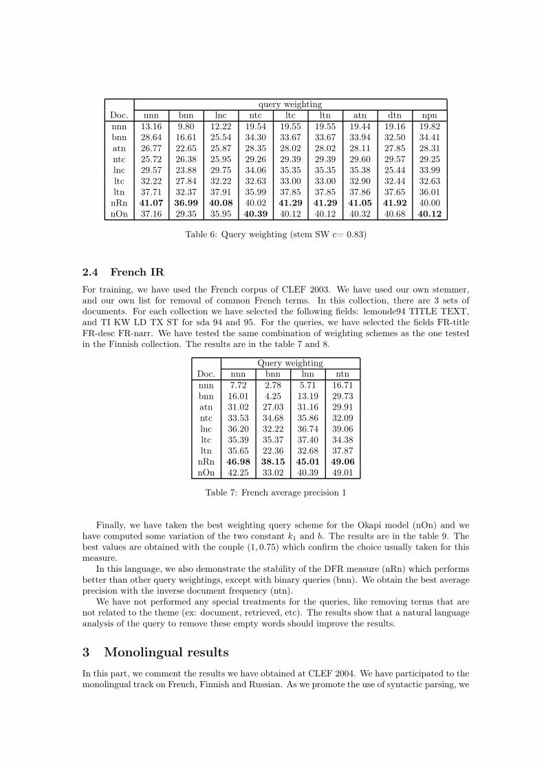
Results of DFR test with nnn query weighting scheme is in the table 5. When c is zero, thenthe equation becomes (4), where term weight are all equal for all documents.

run nRn nnn c=2 ret_rel (483)raw 29.89 388SW 35.39 429

stem SW 39.26 452

Table 4: Test weighting nRn nnn

When we examine DFR formula, one can see that when a term does not appear in documentd, then only di,j is null. Then d∗i,j is also equal to zero. If we strictly apply the formula in thatcase, the weight of the term is still not null and is equal to the formula (4). For practical reason,we have replaced this residual value by zero. This approximation reduces the size of the inversefile, because we do not store null values in file. In fact we have applied the following weighting:

w′i,j =

{wi,j if di,j �= 00 if di,j = 0 (3)

Table 5 show results for some variation in the constant c.We can notice that optimum value is about c = 0.84. This optimization gain 1.21 points

referring neutral value c = 1. One can also notice that we obtain more documents in the first 1000answer for c = 2, but the average precision is lower, which means that they are not well sorted.

wt,d = log2(1 + λt).ft + 1

nt(4)

The conclusion of the use of this weighting is that a good constant c value seems to be 0.83.In the rest of the test, we will use the approximated value c = 0.8.

For the Okapi weighting, we have use the same value as in [1], that is k1 = 1.2, and b = 0.75.In table 9, we have also tested some other value for the French collection: it seems these valuesare on average good ones.

2.3.1 Testing query weighting

We have tested all combination of the following weight:1http://www.unine.ch/info/clef

c precision ret_rel (483)0.00 4.89 2860.10 30.24 4360.50 39.63 4480.70 40.40 4480.75 40.90 4490.80 40.97 4490.81 41.04 4490.82 41.06 4490.83 41.07 4490.84 41.07 4490.85 41.02 4490.86 41.01 4490.87 41.02 4500.90 40.16 4500.95 39.98 4501.00 39.86 4501.50 39.41 4512.00 39.26 4525.00 39.03 44910.0 37.96 447

Table 5: Variation of c for nRn nnn (stem AD)

nnn: Only the term frequency is used.

bnn: This is the binary model. Terms presents are associated to the value 1, and 0 otherwise.

lnc: The cosine is the finale normalization. When both used in document and queries, it ensuretrue vector space model matching, ie. only angle between query et document vector is used.This weighting suppose a log distribution of frequency.

ntc: This is the classical tf*idf measure. We used with queries, the idf is taken from the documentcollection, not the query collection.

ltc: The same classical measure using log on term frequency.

ltn: The log tf*idf without the cosine normalization.

atn: Normalization with the local maximum term frequency is used with idf.

dtn: The double natural log is used in place of the simple one in ltn.

npn: It is the idf variant use for the Okapi system.

nRn: This is the name for Derivation from randomness.

nOn: This is the name for the Okapi probabilistic weighting.

Results are sum up in the table 6.We notice that the derivation from randomness model is very stable again the query weighting

and that it has the best results in the majority of query weighting. We have the decided to use itfor CLEF 2004 in all tests.

query weightingDoc. nnn bnn lnc ntc ltc ltn atn dtn npnnnn 13.16 9.80 12.22 19.54 19.55 19.55 19.44 19.16 19.82bnn 28.64 16.61 25.54 34.30 33.67 33.67 33.94 32.50 34.41atn 26.77 22.65 25.87 28.35 28.02 28.02 28.11 27.85 28.31ntc 25.72 26.38 25.95 29.26 29.39 29.39 29.60 29.57 29.25lnc 29.57 23.88 29.75 34.06 35.35 35.35 35.38 25.44 33.99ltc 32.22 27.84 32.22 32.63 33.00 33.00 32.90 32.44 32.63ltn 37.71 32.37 37.91 35.99 37.85 37.85 37.86 37.65 36.01nRn 41.07 36.99 40.08 40.02 41.29 41.29 41.05 41.92 40.00nOn 37.16 29.35 35.95 40.39 40.12 40.12 40.32 40.68 40.12

Table 6: Query weighting (stem SW c= 0.83)

2.4 French IRFor training, we have used the French corpus of CLEF 2003. We have used our own stemmer,and our own list for removal of common French terms. In this collection, there are 3 sets ofdocuments. For each collection we have selected the following fields: lemonde94 TITLE TEXT,and TI KW LD TX ST for sda 94 and 95. For the queries, we have selected the fields FR-titleFR-desc FR-narr. We have tested the same combination of weighting schemes as the one testedin the Finnish collection. The results are in the table 7 and 8.

Query weightingDoc. nnn bnn lnn ntnnnn 7.72 2.78 5.71 16.71bnn 16.01 4.25 13.19 29.73atn 31.02 27.03 31.16 29.91ntc 33.53 34.68 35.86 32.09lnc 36.20 32.22 36.74 39.06ltc 35.39 35.37 37.40 34.38ltn 35.65 22.36 32.68 37.87nRn 46.98 38.15 45.01 49.06nOn 42.25 33.02 40.39 49.01

Table 7: French average precision 1

Finally, we have taken the best weighting query scheme for the Okapi model (nOn) and wehave computed some variation of the two constant k1 and b. The results are in the table 9. Thebest values are obtained with the couple (1, 0.75) which confirm the choice usually taken for thismeasure.

In this language, we also demonstrate the stability of the DFR measure (nRn) which performsbetter than other query weightings, except with binary queries (bnn). We obtain the best averageprecision with the inverse document frequency (ntn).

We have not performed any special treatments for the queries, like removing terms that arenot related to the theme (ex: document, retrieved, etc). The results show that a natural languageanalysis of the query to remove these empty words should improve the results.

3 Monolingual resultsIn this part, we comment the results we have obtained at CLEF 2004. We have participated to themonolingual track on French, Finnish and Russian. As we promote the use of syntactic parsing, we

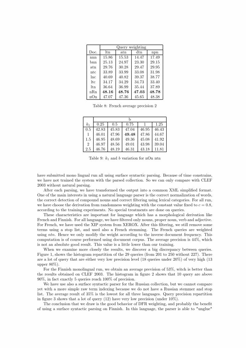
Query weightingDoc. ltn atn dtn npnnnn 15.86 15.53 14.47 17.49bnn 25.13 24.97 23.30 29.15atn 29.76 30.28 29.47 29.95ntc 33.89 33.99 33.08 31.98lnc 40.69 40.82 39.37 38.77ltc 34.17 34.29 34.73 33.40ltn 36.64 36.99 35.44 37.89nRn 48.16 48.76 47.03 48.78nOn 47.07 47.36 45.65 48.38

Table 8: French average precision 2

bk1 0.25 0.5 0.75 1 1.250.5 42.83 45.83 47.04 46.95 46.431 46.01 47.96 49.48 47.86 44.67

1.5 46.95 48.69 49.36 45.08 41.922 46.97 48.56 49.01 43.98 39.04

2.5 46.76 48.19 46.31 43.18 11.81

Table 9: k1 and b variation for nOn ntn

have submitted mono lingual run all using surface syntactic parsing. Because of time constrains,we have not trained the system with the parsed collection. So we can only compare with CLEF2003 without natural parsing.

After each parsing, we have transformed the output into a common XML simplified format.One of the main interests in using a natural language parser is the correct normalization of words,the correct detection of compound nouns and correct filtering using lexical categories. For all run,we have choose the derivation from randomness weighting with the constant value fixed to c = 0.8,according to the training experiments. No special treatments are done on queries.

These characteristics are important for language which has a morphological derivation likeFrench and Finnish. For all language, we have filtered only nouns, proper noun, verb and adjective.For French, we have used the XIP system from XEROX. After this filtering, we still remove someterms using a stop list, and used also a French stemming. The French queries are weightedusing ntn. Hence we only modify the weight according to the inverse document frequency. Thiscomputation is of course performed using document corpus. The average precision is 44%, whichis not an absolute good result. This value is a little lower than our training.

When we examine more closely the results, we discover a big discrepancy between queries.Figure 1, shows the histogram repartition of the 29 queries (from 201 to 250 without 227). Thereare a lot of query that are either very low precision level (18 queries under 20%) of very high (13upper 80%).

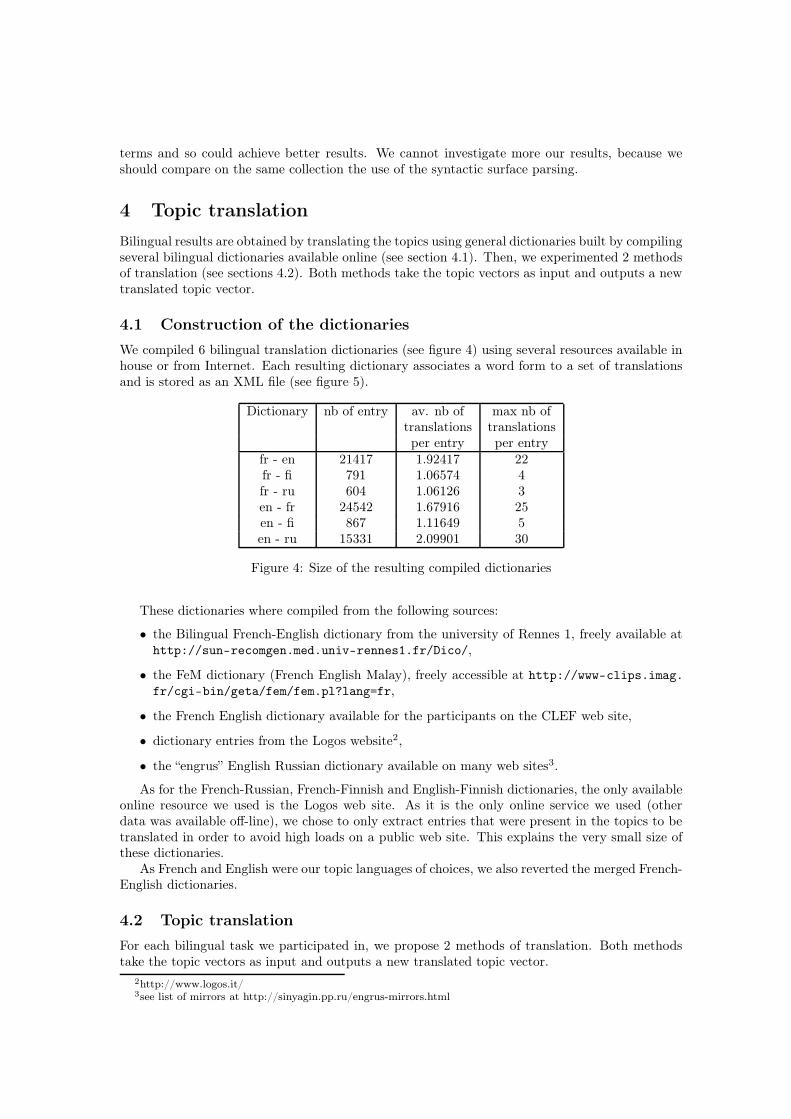
For the Finnish monolingual run, we obtain an average prevision of 53%, witch is better thanthe results obtained on CLEF 2003. The histogram in figure 2 shows that 10 query are above90%, in fact exactly 5 queries reach 100% of precision.

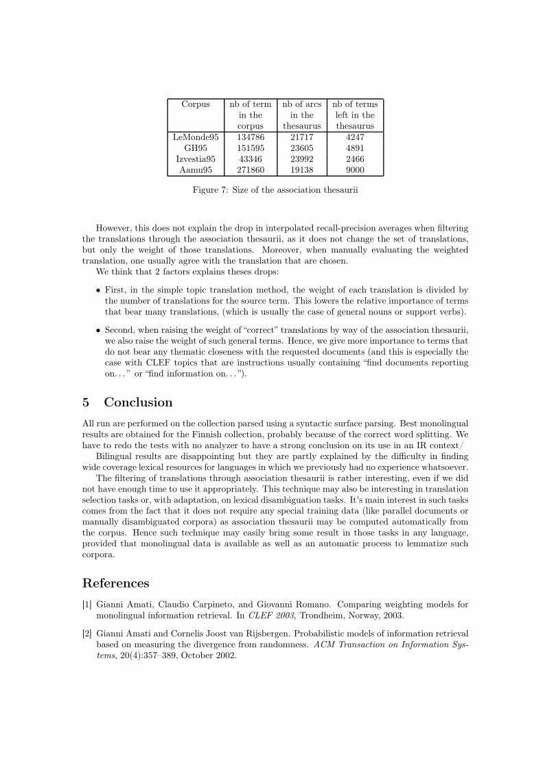
We have use also a surface syntactic parser for the Russian collection, but we cannot compareyet with a more simple raw term indexing because we do not have a Russian stemmer and stoplist. The average result of 35% is the lowest for all three languages. Query precision repartitionin figure 3 shows that a lot of query (12) have very low precision (under 10%).

The conclusion that we draw is the good behavior of DFR weighting, and probably the benefitof using a surface syntactic parsing on Finnish. In this language, the parser is able to "unglue"

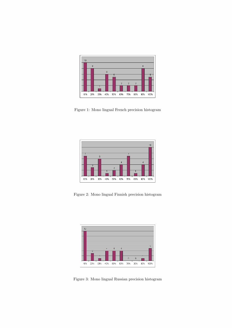
Figure 1: Mono lingual French precision histogram

Figure 2: Mono lingual Finnish precision histogram

Figure 3: Mono lingual Russian precision histogram

terms and so could achieve better results. We cannot investigate more our results, because weshould compare on the same collection the use of the syntactic surface parsing.

4 Topic translationBilingual results are obtained by translating the topics using general dictionaries built by compilingseveral bilingual dictionaries available online (see section 4.1). Then, we experimented 2 methodsof translation (see sections 4.2). Both methods take the topic vectors as input and outputs a newtranslated topic vector.

4.1 Construction of the dictionariesWe compiled 6 bilingual translation dictionaries (see figure 4) using several resources available inhouse or from Internet. Each resulting dictionary associates a word form to a set of translationsand is stored as an XML file (see figure 5).

Dictionary nb of entry av. nb of max nb oftranslations translationsper entry per entry

fr - en 21417 1.92417 22fr - fi 791 1.06574 4fr - ru 604 1.06126 3en - fr 24542 1.67916 25en - fi 867 1.11649 5en - ru 15331 2.09901 30

Figure 4: Size of the resulting compiled dictionaries

These dictionaries where compiled from the following sources:

• the Bilingual French-English dictionary from the university of Rennes 1, freely available athttp://sun-recomgen.med.univ-rennes1.fr/Dico/,

• the FeM dictionary (French English Malay), freely accessible at http://www-clips.imag.fr/cgi-bin/geta/fem/fem.pl?lang=fr,

• the French English dictionary available for the participants on the CLEF web site,

• dictionary entries from the Logos website2,

• the “engrus” English Russian dictionary available on many web sites3.

As for the French-Russian, French-Finnish and English-Finnish dictionaries, the only availableonline resource we used is the Logos web site. As it is the only online service we used (otherdata was available off-line), we chose to only extract entries that were present in the topics to betranslated in order to avoid high loads on a public web site. This explains the very small size ofthese dictionaries.

As French and English were our topic languages of choices, we also reverted the merged French-English dictionaries.

4.2 Topic translationFor each bilingual task we participated in, we propose 2 methods of translation. Both methodstake the topic vectors as input and outputs a new translated topic vector.

2http://www.logos.it/3see list of mirrors at http://sinyagin.pp.ru/engrus-mirrors.html

English to Russian English to French

<entry id="issue"><equiv>выпускать</equiv><equiv>выпуск</equiv><equiv>излияние</equiv><equiv>результат</equiv><equiv>исход</equiv><equiv>спорный_вопрос</equiv><equiv>исходить</equiv><equiv>вытекать</equiv><equiv>вытекание</equiv><equiv>издать</equiv><equiv>издание</equiv><equiv>происходить</equiv><equiv>vypuskat’</equiv><equiv>выход</equiv><equiv>потомство</equiv>

</entry><entry id="harp">

<equiv>арфа</equiv><equiv>играть_на_арфе</equiv>

</entry>

<entry id="issue"><equiv>numero</equiv><equiv>emettre</equiv><equiv>emission</equiv><equiv>matiere</equiv><equiv>delivrer</equiv><equiv>creer</equiv><equiv>affliger</equiv><equiv>impression</equiv><equiv>question</equiv><equiv>delivrance</equiv><equiv>lignee</equiv>

</entry><entry id="harp">

<equiv>harpe</equiv></entry>

Figure 5: Resulting compiled dictionaries sample

4.2.1 Simple topic translation

The first method substitutes each term by all of its available translations. The weight associatedto each translation is equal to the weight of the original term divided by the number of availabletranslation (see figure 6).

4.2.2 Filtering by way of an association thesaurus

As one may see in figure 5, many different translations may be found for a single term. Hence,we tried to develop a strategy to give more importance to the “correct” translation(s). For this,we tried to take some context into account, without changing anything to the available lexicalresource.

For this, we needed contextual information in each language. Hence, we automatically builtan association thesaurus (as exposed in [3]) for each language from the available monolingualdocuments (see figure 7).

Each association thesaurus is as a graph linking terms. Each arc in the graph links 2 termsthat “regularly”4 appear in the same context. For this experiment, 2 terms are said to be in thesame context when they appear in the same document.

For our experiment, we assume that terms that are close to each others share some commonsemantic. We also assume that their “correct” translations should also share the same semantic.Hence, we used these association thesaurus to know if terms and translations share some semantics.Hence, we chose to associate each translations ti,j of a term cj with a weight wti,j depending onits distance (dti,j ) with the translated context. The distance of a translation to the translatedcontext is given by formula 5.

4In this experiment, we filtered out arcs that had a confidence score lower than 20% or higher than 90%.

Original vector (en) Translated Vector (ru)

<vector id="C250" size="17"><c id="Rabie" w="1"/><c id="allow" w="1"/><c id="be" w="1"/><c id="discussing" w="1"/><c id="document" w="3"/><c id="find" w="1"/><c id="human" w="5"/><c id="incident" w="2"/><c id="interest" w="1"/><c id="learn" w="1"/><c id="method" w="2"/><c id="prevention" w="2"/><c id="rabies" w="4"/><c id="reader" w="1"/><c id="relevant" w="1"/><c id="reporting" w="2"/><c id="use" w="1"/></vector>

<vector id="C250" size="57">...<!-- Translation of id="reader" w="1" --><c id="reader" w="1" untranslated="true"/><!-- Translation of id="human" w="5" --><c id="ЧЕЛОВЕЧЕСКИЙ" w="2.5"/><c id="ЧЕЛОВЕК" w="2.5"/><!-- Translation of id="document" w="3" --><c id="ПОДТВЕРЖДАТЬ_ДОКУМЕНТАМИ" w="1"/><c id="ДОКУМЕНТ" w="1"/><c id="СВИДЕТЕЛЬСТВО" w="1"/><!-- Translation of id="Rabie" w="1" --><c id="Rabie" w="1" untranslated="true"/><!-- Translation of id="prevention" w="2" --><c id="prevention" w="2" untranslated="true"/><!-- Translation of id="interest" w="1" --><c id="ИНТЕРЕС" w="0.25"/><c id="ВЫГОДА" w="0.25"/><c id="ИНТЕРЕСОВАТЬ" w="0.25"/><c id="ЗАИНТЕРЕСОВЫВАТЬ" w="0.25"/><!-- Translation of id="rabies" w="4" --><c id="БЕШЕНСТВО" w="4"/>...</vector>

Figure 6: Simple topic translation

dti,j = Min(d(ti,j , tk,l); ∀l, k | l �= j, 1 ≤ k ≤ [Tl|)where tk,l ∈ Tl

and Tl is the set of translation of the term cl

and d(ti,j , tk,l) is the minimal distance in the target thesaurus between ti,j and tk,l

(5)

wti,j ={

wj/di,j if di,j �= 0wj/|Tj| if di,j = 0

where wj is the weight of the source term cj in the source vector(6)

Figure 8 shows a sample resulting translated vector. One may notice the higher weight of theselected translations (e.g. interest → ИНТЕРЕС).

4.3 DiscussionCLIPS results on the bilingual tasks are rather disappointing, with interpolated recall-precisionaverages at 0.00 dropping from 57.68% (Monolingual Russian) to 17.1% with simple topic transla-tion (Bilingual English-Russian: CLIPSENRU1) and even to 8.59% with filtered topic translation(CLIPSENRU2).

The main reason for this drop is certainly due to the lack of wide coverage bilingual lexicalresources. The dictionaries we used were very small and did not provide translations for manyterms of the topics. This is especially true for French to Russian and Finnish lexical resourceswhere 60% to 70% of the source terms are not translated. However, English to Russian lexiconwas a little better, and about 18% of the terms remain without translation.

Corpus nb of term nb of arcs nb of termsin the in the left in thecorpus thesaurus thesaurus

LeMonde95 134786 21717 4247GH95 151595 23605 4891

Izvestia95 43346 23992 2466Aamu95 271860 19138 9000

Figure 7: Size of the association thesaurii

However, this does not explain the drop in interpolated recall-precision averages when filteringthe translations through the association thesaurii, as it does not change the set of translations,but only the weight of those translations. Moreover, when manually evaluating the weightedtranslation, one usually agree with the translation that are chosen.

We think that 2 factors explains theses drops:

• First, in the simple topic translation method, the weight of each translation is divided bythe number of translations for the source term. This lowers the relative importance of termsthat bear many translations, (which is usually the case of general nouns or support verbs).

• Second, when raising the weight of “correct” translations by way of the association thesaurii,we also raise the weight of such general terms. Hence, we give more importance to terms thatdo not bear any thematic closeness with the requested documents (and this is especially thecase with CLEF topics that are instructions usually containing “find documents reportingon. . . ” or “find information on. . . ”).

5 ConclusionAll run are performed on the collection parsed using a syntactic surface parsing. Best monolingualresults are obtained for the Finnish collection, probably because of the correct word splitting. Wehave to redo the tests with no analyzer to have a strong conclusion on its use in an IR context/

Bilingual results are disappointing but they are partly explained by the difficulty in findingwide coverage lexical resources for languages in which we previously had no experience whatsoever.

The filtering of translations through association thesaurii is rather interesting, even if we didnot have enough time to use it appropriately. This technique may also be interesting in translationselection tasks or, with adaptation, on lexical disambiguation tasks. It’s main interest in such taskscomes from the fact that it does not require any special training data (like parallel documents ormanually disambiguated corpora) as association thesaurii may be computed automatically fromthe corpus. Hence such technique may easily bring some result in those tasks in any language,provided that monolingual data is available as well as an automatic process to lemmatize suchcorpora.

References[1] Gianni Amati, Claudio Carpineto, and Giovanni Romano. Comparing weighting models for

monolingual information retrieval. In CLEF 2003, Trondheim, Norway, 2003.

[2] Gianni Amati and Cornelis Joost van Rijsbergen. Probabilistic models of information retrievalbased on measuring the divergence from randomness. ACM Transaction on Information Sys-tems, 20(4):357–389, October 2002.

Original vector (en) Translated Vector (ru)

<vector id="C250" size="17"><c id="Rabie" w="1"/><c id="allow" w="1"/><c id="be" w="1"/><c id="discussing" w="1"/><c id="document" w="3"/><c id="find" w="1"/><c id="human" w="5"/><c id="incident" w="2"/><c id="interest" w="1"/><c id="learn" w="1"/><c id="method" w="2"/><c id="prevention" w="2"/><c id="rabies" w="4"/><c id="reader" w="1"/><c id="relevant" w="1"/><c id="reporting" w="2"/><c id="use" w="1"/></vector>

<vector id="C250" size="57">...<!-- Translation of id="reader" w="1" --><c id="reader" w="1" untranslated="true"/><!-- Translation of id="human" w="5" --><c id="ЧЕЛОВЕЧЕСКИЙ" w="2.5"/><c id="ЧЕЛОВЕК" w="5"/><!-- Translation of id="document" w="3" --><c id="ПОДТВЕРЖДАТЬ_ДОКУМЕНТАМИ" w="1"/><c id="ДОКУМЕНТ" w="1"/><c id="СВИДЕТЕЛЬСТВО" w="1"/><!-- Translation of id="Rabie" w="1" --><c id="Rabie" w="1" untranslated="true"/><!-- Translation of id="prevention" w="2" --><c id="prevention" w="2" untranslated="true"/><!-- Translation of id="interest" w="1" --><c id="ИНТЕРЕС" w="0.5"/><c id="ВЫГОДА" w="0.25"/><c id="ИНТЕРЕСОВАТЬ" w="0.25"/><c id="ЗАИНТЕРЕСОВЫВАТЬ" w="0.25"/><!-- Translation of id="rabies" w="4" --><c id="БЕШЕНСТВО" w="4"/>...</vector>

Figure 8: Topic translation with filtering

[3] Jean-Pierre Chevallet and Gilles Serrasset. Simple translations of monolingual queries ex-panded through an association thesaurus. x-iota ir system used for clips bilingual experiments.In CLEF 2003, 2003.

[4] S. E. Robertson. Overview of the okapi projects. Journal of Documentation, 53(1):3–7, 1997.

[5] Steve E. Robertson, S. Walker, and Micheline Baulieu. Okapi at trec-7: Automatic ad hoc,filtering, vlc and interactive track. In Preceedings of TREC-7, 1998.