The brain matures with stronger functional connectivity and decreased randomness of its network

The Brain Matures with Stronger Functional Connectivityand Decreased Randomness of Its Network

Dirk J. A. Smit1,3*, Maria Boersma2, Hugo G. Schnack4, Sifis Micheloyannis5, Dorret I. Boomsma1,3,6,

Hilleke E. Hulshoff Pol4, Cornelis J. Stam2,3, Eco J. C. de Geus1,3,6

1 Biological Psychology, VU University, Amsterdam, The Netherlands, 2Clinical Neurophysiology, VU Medical Centre, Amsterdam, The Netherlands, 3Neuroscience

Campus Amsterdam, VU University, Amsterdam, The Netherlands, 4Department of Psychiatry, University Medical Center Utrecht, Utrecht, The Netherlands, 5Clinical

Neurophysiology Laboratory L Widen, University of Crete, Iraklion, Greece, 6 EMGO+ Institute, VU Medical Centre, Amsterdam, The Netherlands

Abstract

We investigated the development of the brain’s functional connectivity throughout the life span (ages 5 through 71 years)by measuring EEG activity in a large population-based sample. Connectivity was established with SynchronizationLikelihood. Relative randomness of the connectivity patterns was established with Watts and Strogatz’ (1998) graphparameters C (local clustering) and L (global path length) for alpha (,10 Hz), beta (,20 Hz), and theta (,4 Hz) oscillationnetworks. From childhood to adolescence large increases in connectivity in alpha, theta and beta frequency bands werefound that continued at a slower pace into adulthood (peaking at ,50 yrs). Connectivity changes were accompanied byincreases in L and C reflecting decreases in network randomness or increased order (peak levels reached at ,18 yrs). Olderage (55+) was associated with weakened connectivity. Semi-automatically segmented T1 weighted MRI images of 104young adults revealed that connectivity was significantly correlated to cerebral white matter volume (alpha oscillations:r = 33, p,01; theta: r = 22, p,05), while path length was related to both white matter (alpha: max. r = 38, p,001) and graymatter (alpha: max. r = 36, p,001; theta: max. r = 36, p,001) volumes. In conclusion, EEG connectivity and graph theoreticalnetwork analysis may be used to trace structural and functional development of the brain.

Citation: Smit DJA, Boersma M, Schnack HG, Micheloyannis S, Boomsma DI, et al. (2012) The Brain Matures with Stronger Functional Connectivity and DecreasedRandomness of Its Network. PLoS ONE 7(5): e36896. doi:10.1371/journal.pone.0036896

Editor: Pedro Antonio Valdes-Sosa, Cuban Neuroscience Center, Cuba

Received November 8, 2011; Accepted April 9, 2012; Published May 15, 2012

Copyright: � 2012 Smit et al. This is an open-access article distributed under the terms of the Creative Commons Attribution License, which permits unrestricteduse, distribution, and reproduction in any medium, provided the original author and source are credited.

Funding: This research was supported by VU University Universitair Stimuleringsfonds (VU-USF 96/22), Human Frontiers of Science Program (RG0154/1998-B),Netherlands Organization for Scientific Research (NWO/SPI 56-464-14192 to D.B., NWO/MagW VENI-451-08-026 to D.S.). The funders had no role in study design,data collection and analysis, decision to publish, or preparation of the manuscript.

Competing Interests: The authors have declared that no competing interests exist.

* E-mail: [email protected]

Introduction

The brain is a complex network of highly connected brain areas

that exchange information via long-range axonal projections.

Several methods are available to investigate connectivity. Ana-

tomical methods include Diffusion Tensor Imaging tract tracin

[1,2] and connectivity derived from cortical gray matter thicknes

[3,4]. Functional methods use direct (EEG, MEG) or indirect

(fMRI BOLD) measures of correlated neuronal activity to derive

networks of functionally coupled brain areas. fMRI is a measure

with a high spatial resolution which has been found to consistently

extract subnetworks in the brain that show activity modulation on

a time-scale of tens of seconds (Resting state network [5,6]). MEG/

EEG, on the other hand, may be used to estimate short duration

networks that arise and disappear on a scale of seconds, although it

has been shown that both types of resting state networks share a

common groun [7,8].

In addition to establishing overall brain connectivity, graph

theoretical analysis allows the evaluation of whole-brain efficienc

[9] and the determination of network topologies, such as small-

world network [10–12]. Networks can be classified as ordered,

small world, or random by the use of two graph parameters,

clustering coefficient C and path length [13,14]. Watts and Strogat

[12] showed that highly ordered networks (high C) with only a few

random links could achieve optimal connectivity (short L) close to

the random state. These small-world networks have favorable

properties with efficient information transfer and resilience to

(simulated) attack [10,15–17]. Confirming this evolutionary

advantage, human brains were shown to have this small-world

topolog [15,18], which indeed favors cognitive performanc

[19,20]. Interestingly, people differ systematically in the graph

parameters and these differences are geneti [21,22]. In addition,

deviant graph parameters have been found in disease states

compared to control [23–25] which might therefore act as markers

for developmental psychopathology or neurodegeneration.

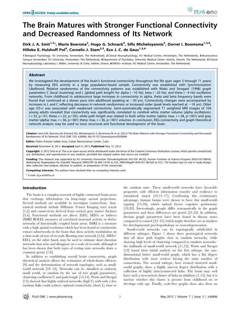
Small-world networks can be topologically subdivided in

different subtypes. Figure 1 shows three prototypical networks

that all show path lengths close to random networks, while

showing high levels of clustering compared to random networks–

the hallmark of small-world network [11,12]. Watts and Strogat

[12] based their initial analysis on the first subtype, the one-

dimensional lattice small-world graph, which has a flat degree

distribution with most vertices having the same number of

connections. The second subtype, here termed clustered small-

world graphs, show a highly uneven degree distribution with a

collection of highly (inter)connected hubs. The brain may well

have such a neocortical cluster of hubs in adulthoo [1,15], but it is

unclear whether this cluster is present from childhood on or

develops with age. Finally, scale-free graphs show also show an

PLoS ONE | www.plosone.org 1 May 2012 | Volume 7 | Issue 5 | e36896

uneven degree distribution, but with exponentially increasing

number of connections. This graph subtype shows the highest level

of skew in the degree distribution, and may be less optimal

evolutionary because of the vulnerability to targeted attack [14].

Although the graph parameters C and L make statements about

network quality along the dimension of random – small world –

ordered, they may not reveal these qualitative topological

differences and their development over time [26]: All of the above

networks, although in different degrees, show small-world

properties of a relatively high C and short L. This topological

network quality may be revealed by inspecting the number of

connection each vertex (node) has: the degree distribution K = {k1,

k2, …, kN} where ki holds the number of connections for each

vertex i =,1, N. sorted from low to high. Inspection of the

degree distribution of networks in different age groups can reveal

these qualitative changes–such as the development of cortical

hubs–thus providing insight into the underlying growth rules

underlying the neural network developmen [27].

In this study, we used EEG in relative short (12 s) periods to

establish synchronization between EEG signals from relatively

distant brain areas, thus reflecting long-range connectivity. We did

this in a sample spanning a large age range (5 to 71) so that we

could chart the development of functional connectivity and degree

of order assessed from graph parameters across the life span. As a

second aim we tested whether the brain network changes its

topological quality over time, in addition to its degree of order.

Brain maturation involves marked changes in anatomical struc-

ture, including an initial increase into childhood and subsequent

continuous decrease in gray matter volume as well as density, the

protracted increase of white matter volume, and decline of

fractional anisotrop [28–33], as a result of synaptic density changes

(pruning), myelination, and axonal diameter change [34]. As a

final aim we investigated whether brain anatomy was correlated

with the observed differences in functional connectivity–and the

graph parameters derived from these networks–by correlating

these with cerebral white matter volume (WMV) and gray matter

volume (GMV) established from MRI scans available in a young

adult subset of the subjects. Although restricted to one age group, a

correlation between functional connectivity, network randomness,

and underlying anatomical variables may prove helpful in

understanding how the observed large changes in brain anato-

my–including both young developmen [30,34,35] and agin

[33,36,37]– shapes brain activity and, ultimately, brain function.

Methods

Subjects and procedureData were collected as part of an ongoing study into the genetics

of brain development and cognition. A total number of 1675

individuals (twins and additional siblings) accepted an invitation

for extensive EEG measurement. For the present analyses, EEG

data recorded during 3–4 minutes of eyes-closed rest were

available from six measurement waves with ages centered around

5, 7, 16, 18, 25, and 50 years. Part of these consisted of

longitudinal measurements at two ages (5–7 and 16–18 years).

In addition, some of the subjects aged 16–18 years were invited

back for measurements at age 25. In total, this study incorporated

2540 EEG recordings. After data cleaning, 2137 datasets were

available. The structure of the final subject set after data cleaning

used in the present study was 331, 368, 418, 380, 350, and 290 for

the six measurement waves, which included 294 longitudinal

observations between 5 and 7, 374 between 16 and 18, 96 between

18 and 25, of which 95 with measurements at three waves 16, 18,

and 25.

Ethical permission was obtained via the "subcommissie voor de

ethiek van het mensgebonden onderzoek" of the Academisch

Ziekenhuis VU (currently named METc of the VUmc). All

subjects (and parents/guardians for subjects under 18) were

informed about the nature of the research. All subjects or parents/

guardians were invited by letter to participate, and agreement to

participate was obtained in writing. All subjects were treated in

accordance with the Declaration of Helsinki.

EEG acquisitionThe childhood and adolescent EEG were recorded with tin

electrodes in an ElectroCap connected to a Nihon Koden PV-

441A polygraph with time constant 5 s (corresponding to a

0.03 Hz high-pass filter) and lowpass of 35 Hz, digitized at

250 Hz using an in-house built 12-bit A/D converter board and

stored for offline analysis. Leads were Fp1, Fp2, F7, F3, F4, F8,

C3, C4, T5, P3, P4, T6, O1, O2, and bipolar horizontal and

vertical EOG derivations. Electrode impedances were kept below

5 kV. Following the recommendation by Pivik et al.[38], tin

earlobe electrodes (A1, A2) were fed to separate high-impedance

amplifiers, after which the electrically linked output signals served

Figure 1. Degree distributions of prototypical networks. Rightcolumn shows illustrations of prototypical networks: the (ring) latticesmall-world, the clustered small-world, and the scale-free network. Notethat all ordered networks have small world properties as C.1.0 andL,1.0, albeit to a different degree. Random networks serve as baselinefor all comparisons (C = 1.0 and L = 1.0). From the three types of orderednetworks, graphs (number of vertices: N = 14, average degree =average number of connections per vertex: K = 4.0) were simulated withthree random reconnections to ensure small-world properties. Theresulting degree distribution holds the number of connections sortedlow to high (Top left plot) with the dashed line representing theaverage of 1000 randomized graphs. The three types of ordered graphsshow highly distinctive degree distributions when plotted relative tothe random graph (bottom left plot). Lattice small-world networks haverelative flat degree distribution (around 4) resulting in a negative slopewhen compared to random networks. Clustered small-world networkshave one set of vertices with low degree, another with high degreeresulting in a rotated-S-shaped curve. Scale-free networks have aexponentially increasing curve in their degree distribution.doi:10.1371/journal.pone.0036896.g001

Development of Brain Connectivity


as reference to the EEG signals. Sine waves of 100 mV were used

for calibration of the amplification/AD conversion before

measurement of each subject.

Young adult and middle-aged EEG was recorded with Ag/

AgCl electrodes mounted in an ElectroCap and registered using

an AD amplifier developed by Twente Medical Systems (TMS;

Enschede, The Netherlands) for 657 subjects and NeuroScan

SynAmps 5083 amplifier for 103 subjects. Standard 10–20

positions were F7, F3, F1, Fz, F2, F4, F8, T7, C3, Cz, C4, T8,

P7, P3, Pz, P4, P8, O1 and O2. For subjects measured with

NeuroScan Fp1, Fp2, and Oz were also recorded. The vertical

electro-oculogram (EOG) was recorded bipolarly between two

Ag/AgCl electrodes, affixed one cm below the right eye and one

cm above the eyebrow of the right eye. The horizontal EOG was

recorded bipolarly between two Ag/AgCl electrodes affixed one

cm left from the left eye and one cm right from the right eye. An

Ag/AgCl electrode placed on the forehead was used as a ground

electrode. Impedances of all EEG electrodes were kept below

3 kV, and impedances of the EOG electrodes were kept below

10 kV. The EEG was amplified, digitized at 250 Hz and stored for

offline processing.

EEG preprocessingWe selected 14 EEG signals (Fp1, Fp2, F7, F3, F4, F8, C3, C4,

T5, P3, P4, T6, O1, O2 and both EOG channels) for further

analysis. For subjects without Fp1 and Fp2 recordings, these were

substituted with their closest match F1 and F2. The reason for this

lead replacement was that a reduced (12 lead) graph yielded graph

parameters much closer to random values, with a reduced power

to detect age differences. This substitution was tested by

comparing 46 unrelated individuals who had both F1, F2 and

Fp1, Fp2 sets available. The correlations r(CF1F2, CFp1Fp2), r(LF1F2,

LFp1Fp2), and r(SLF1F2, SLFp1Fp2) were very high (.93.r.96 for

alpha oscillations, .75 ,r,.97 for beta oscillations). Even though

correlations were high, the C, L, and SL scores showed a small but

systematic bias (,.043 for C, ,054 for L, and ,15 for SL). This

bias was removed in all subsequent scoring.

All signals were broadband filtered from 1 to 37 Hz with a zero-

phase FIR filter with 6dB roll-off. Next, we visually inspected the

traces and removed bad signals. Note that for the network analysis

a full set of EEG signals was required and therefore any rejected

EEG channel resulted in the loss of that subject. Next, we used the

extended ICA decomposition implemented in EEGLA [39] to

remove artifacts, including eye movements, and blink [40]. After

exclusion of components reflecting artifacts, the EEG signals were

filtered into the alpha (6.0 to 13.0 Hz) and beta (15.0 to 25.0 Hz)

frequency bands. The peak alpha frequency developed from

8.1 Hz at age 5 to 9.9 Hz at age 18, after which a slow decline to

9.4 Hz was observed at around 50 years. The lower edge of the

alpha filter was set such that alpha oscillation of all subjects was

included from ,2.0 Hz below the lowest peak frequency to

,3.0 Hz above the highest peak frequency. EEG power in the

defined theta, alpha, and beta frequency bands was determined

using Welch’ method on 50% overlapping stretches of 4096

samples.

ConnectivityEEG signals are thought to reflect the neural activity of the

brain tissue that results from synchronous dendritic input across a

large cortical area. Connectivity was calculated using synchroni-

zation likelihood (SL) following Stam and van Dij [41]. SL is based

on generalized synchronization between coupled systems removes

the overestimation shown by coherence in filtered signals, and

detects linear as well as non-linear connectivity. In short, if a signal

s1 is in a certain state (to be defined below) at time i we may find a

recurrence of that state at another time point j. Next, we look if the

second signal s2 is in the same state at time points i and j,

recording a hit if so. SL is defined as the proportion of hits (in s2)

to the total number of recurrences (in s1) and is thus a number

between 0 and 1. Note that SL is found even when signals s1 and

s2 are in different states, as long as s1 and s2 are self-similar at i

and j.

More formally, the instantaneous state of an EEG signal was

represented by m-dimensional state vectors Xi = {xi, xi + 1l, xi +

2l, …, xi+(m21)l } where l is the lag and m the embedding

dimension. The elements of Xi are m samples taken from the

signal spaced l apart. The vector is taken to represent the state of

the system at time i. Within the same signal recurrences are sought

at times j that reflect a similar state: A threshold distance e is

chosen such that a fixed proportion (pref =0.02) of comparisons

are close enough to be considered in a similar state. Next, the same

comparison is made for a different system Y at the same time

points i and j and with the same value for pref. Now the

synchronization likelihood Si between X and Y at time i is defined

as follows:

Si~1

N

XN

j~1h e{ Yi{Yj

�

�

�

�

� �

h e{ Xi{Xj

�

�

�

�

� �

where h is the Heaviside step function returning 0 for all values,0

and 1 for values .=0. Time point j is chosen with a minimum lag

from i and depends on the lower value of the filter, so as to avoid

autocorrelation effects. N represents the number of recurrences of

the state Xi within X. Overall SL between X and Y is the average

over all possible i. The settings for SL calculation were those

recommended by Montez et al.[42]. Note that these settings are

not critical in the calculation of S [21].

Graph analysisGraphs were created by thresholding the SL matrices such that

the total number of (bidirectional) connections in the graph was 32

resulting in an average number of connections per vertex (node) of

K= 4.0. Graph parameters clustering coefficient C and path

length L were calculated following Watts and Strogat [12]. In

short, C is calculated for each vertex as the proportion of

neighboring vertices that are interconnected between them. That

is, if vertex v1 is connected with v2 and v3, this constitutes a closed

triangle, and an open triangle if they are not. C is then nclosed/

(nclosed+nopen). Overall graph C is the mean across all Ci, i =,1,

N.. Path length L is also calculated for each vertex, and reflects

the average minimum number of steps required go from the

current vertex to all other vertices, passing only along existing

edges. Note that the averaging procedure for L is the harmonic

mean L=1/sum(1/Li) with unconnected nodes assigned the value

of +‘. This reduces the influence of unconnected nodes while

retaining the full network siz [11]. All C and L scores were

normalized to reflect deviation from randomness by dividing each

score with the average of C and L from 1000 Erdos-Renyi random

graphs with the same number of vertices and average degree as the

empirical graphs. A value of 1.0 therefore reflects a value as in the

random case.

Note that for subjects with replaced leads (F1, F2 in stead of

Fp1, Fp2) we removed the systematic bias as explained above.

Structural MRI AssessmentFrom 104 subjects (62 male; average age 27.4 years) magnetic

resonance imaging (MRI) scans were aquired at a Philips 1.5 T

Intera scanner (Philips, Best, The Netherlands) at the University



Medical Center Utrecht. For a detailed description of the

aquistion and processing of the scans of this sample, see Baare

et al. [43]. In short, the T1-weighted images (voxelsize

16161.2 mm3) were transformed into Talairach orientation (no

scaling) [44] and corrected for magnetic field inhomogeneitie [45].

Segments of gray and white matter of the cerebrum were obtained

by an automated method validated earlie [46], from which tissue

volumes were calculated.

We calculated partial correlations (accounting for sex differenc-

es) between MRI volumes and the EEG parameters. As SL and L

were highly skewed we applied a log transformation and a 21/x

transformation respectively (note that the negation keeps the

direction of the correlation intact) to effectively normalize the

distributions of these variables. C was approximately normally

distributed. Bootstrap resampling was used to calculate confidence

intervals for the partial correlations (see statistics).

StatisticsObservations were split into nine age groups with age

boundaries in years: 4.9 – 6.0, 6.0 – 7.4, 15.0 – 17.0, 17.0 –

20.0, 20.0 – 25.0, 25.0 – 35.0, 35.0 – 45.0, 45.0 – 55.0, and 55+.

These groups were labeled ,5, ,7, ,16, ,18, ,22, ,30, ,40,

,50, and 55+. Final group sizes and average ages are shown in

Table 1.

Because the complex structure of the data including repeated

measures and family dependencies, which even extended across

the different age groups (siblings of twins might fall into a different

age category than the proband twins), we established significance

via bootstrapping. The bootstrap consisted of randomly selecting

(with replacement) from the pool of families, retrieving the data for

all family members, and calculating the statistic (i.e., the difference

in group means) and estimating its confidence interval. Sampling

on the family level rather than individual level keeps–on average–

the complex covariance structure between the family members

and repeated measures intact. Confidence intervals were adjusted

using the bias correction and accelerated metho [47], and a

conservative alpha level of .01 was used. Group differences tested

were limited to adjacent age groups and groups two steps apart.

Results

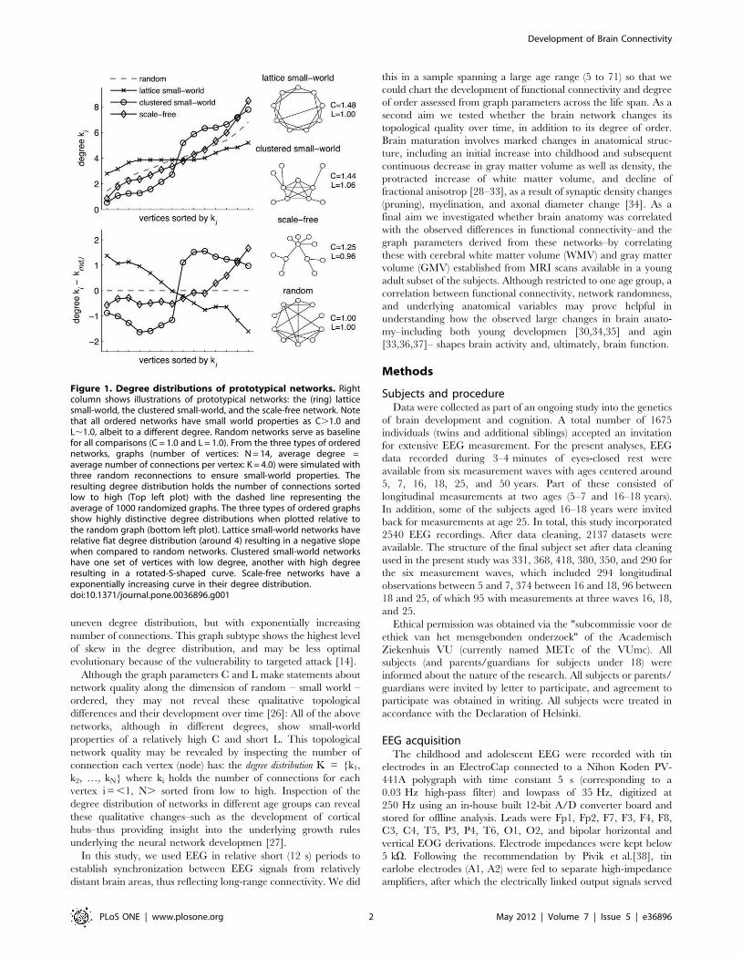
Protracted development of connectivityAll three frequency bands (Figures 2, 3, and 4) showed similar

development of synchronization likelihood (SL) which significantly

increased with age reflecting the prolonged maturation of brain

connectivity. The connectivity enhancement extended well into

adulthood and even into middle-aged adulthood, after which a

plateau developed. All three figures show that peak connectivity

was found at age ,50. A significant decline in connectivity was

only first observed in the 55+ age group for all frequency

oscillations.

Graph parameters revealed large increases in networkorder between childhood and adolescence anddecreases in late adulthoodOverall, the development in C and L shows a change in the

quality of the brain network from a relative random to a more

ordered organization, from childhood to adolescence. Alpha and

beta frequency bands showed evidence for increases in both C and

L between childhood and adolescence (Figures 2, 3, left columns).

Significance of these changes is indicated in the right columns. C

additionally shows a clear increase within adolescence. In

adolescence, a plateau is reached, which is by-and-large

maintained throughout adult life. Only beta band C shows a

significant increase in the oldest age group. Development of theta

networks in early childhood deviated from this pattern, as there

was an initial decrease in connectivity and graph parameter C

from age 5 to 7. This is most likely related to the very large

decrease in theta power during the first decade of life. Significant

increases within adulthood years were observed for L (,30 to

,50), reflecting a relative stability between adolescence and

adulthood for this measure.

Network development in the first two decades of life reach

maximal levels at the age of ,18 for C and L. Older age was

generally associated with decreases in both C and L but these

effects were only significant for L in the theta band. A significant

increase in C was found for networks from beta oscillations.

Figure 5 shows the development of the graph parameters C and

L (alpha oscillations only) as a function of average degree K chosen

in the thresholding procedure. Many age effects were independent

of the choice of K. This indicates a certain generality of the effects

and an independence of the arbitrary choice of K. Childhood is

marked by highly random network connectivity patterns, that

slowly increased to more ordered networks. For all levels of K, the

changes observed between age groups 5 and 7 were minimal

compared to the increase in order from childhood to adolescence.

Adolescence also showed increase in order of the brain network,

but the maximal values for C are reached somewhat earlier than

for L. Finally, older age is characterized by a reversal towards

increased randomness.

Connectivity and network change are unlikely to becaused by spurious power effectsIt could be argued that a lack of connectivity between brain

areas–and a resulting random network configuration–could be the

result not of the absence of connectivity per se, but the absence of

oscillations from which they are derived. Since EEG power density

reflects the amount and strength of the oscillations, the spurious

effect would predict a positive relation between EEG power and

connectivity (or the graph parameters derived from it). Figures 2 to

4 (bottom rows) show that EEG power density of both alpha and

beta oscillations follow a very different developmental trajectory

than the connectivity parameters. In general, they are in the

opposite direction of the spurious effect (i.e., a decrease in power is

associated with an increase in C and L, i.e. a depart from

randomness), giving no support to this alternative explanation.

One notable exception is the strong decrease in theta power

associated with concurrent decreases in C and L. Therefore,

Table 1. Age group definition and size.

Age group (yrs) N Mean (SD) Range

,5 (below 6.0) 331 5.3 (0.19) (4.93–5.86)

,7 (6.0–7.5) 368 6.8 (0.19) (6.45–7.46)

,16 (15.2–17.0) 447 16.1 (0.47) (15.23–16.99)

,18 (17.0–20.0) 345 17.6 (0.39) (17.00–18.92)

,22 (20.0–25.0) 148 23.4 (0.90) (20.21–24.95)

,30 (25.0–35.0) 176 28.6 (2.52) (25.04–34.55)

,40 (35.0–45.0) 96 41.6 (2.33) (35.40–44.99)

,50 (45.0–55.0) 149 48.9 (2.44) (45.32–54.26)

55+(55.0 and older) 55 60.8 (4.14) (55.35–71.03)

doi:10.1371/journal.pone.0036896.t001



concurrent changes in theta power may have caused the deviant

patterns for theta connectivity in the childhood age groups.

Topological network quality is stable for alpha, thetaoscillations but changes for beta oscillationsTopological network quality was next assessed by inspecting the

degree distribution Ki of the brain connectivity graphs, sorted low

to high and averaged over all epochs/subjects. These were plotted

for age groups ,5, ,16, ,22, ,40, and 55+ years (Figure 6), and

can be visually compared with the degree distributions obtained

for the three prototypical ordered graphs of Figure 1. For graphs

from alpha oscillations, it was clear that the networks represented a

clustered small-world network throughout life, as evidenced by the

S-shaped degree distribution. Interestingly, the S-shape did not

qualitatively change, but increased in amplitude, suggesting that

the connectivity within the cluster becomes more pronounced as

age progresses and reaching a plateau already at age ,16.

Therefore, the degree distribution of alpha oscillation networks

shows no evidence for qualitative topological change from ,5 to

,55 years of age.

Figure 2. Alpha band (6–13 Hz) development of Clustering, Path Length, average connectivity, and average power. SL is the averageconnectivity of synchronization likelihood across all possible pairs of signals. Clustering C and Path Length L were obtained as indicated in the text.Dashed lines are values obtained for randomized networks (C and L) or connectivity between two white noise signals (SL). (Left column:) Eachvariable is plotted with a continuous predictor and a quadratic loess smooth 40% of the data. Results show a small-world organization throughout lifeas L,1.0 while C..1.0. Large changes were observed for L, overall connectivity, and less so for C. The opposite development of the power of alphaoscillations suggests that increased order is not a spurious effect of increased signal-to-noise ratios. (Right column:) Means by age group. Hooksindicate bootstrap determined significant difference (gray: p,.01, thin black p,001, thick black p,0001) between adjacent and next-adjacentgroups. Significant increases between childhood and adolescence and even within adolescence (for C) indicate a decrease of brain networkrandomness with age. A stable period for C after,18 and for L after,16 yrs was observed. Overall connectivity significantly increased up to,40 butpeaked at ,50, and showed a significant decrease into older age (55+).doi:10.1371/journal.pone.0036896.g002



A similar clustered topology was obtained for graphs from theta

oscillations. Although the nodes with lowest degree were

somewhat lower than expected, the sorted degree distributions

consistently showed high degree for a subset of nodes and low

degree for the remainder, reflecting the core property of a

clustered network. The topology was quite stable across age

groups.

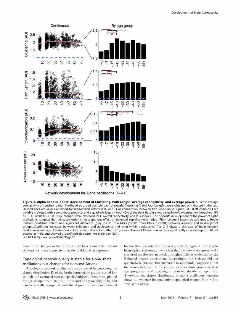
For beta band oscillations, networks represented a flatter degree

distribution than a clustered small-world network with even a

slightly downward slope–an indication of a lattice small-world

network. Childhood, adolescent, and the oldest age groups showed

the flattest degree distribution–an indication of increased random-

ness. This provides some evidence that the beta oscillatory network

is in an immature state before adulthood with an underdeveloped

network cluster. This cluster only reaches full interconnectivity

between the hubs in the cluster at ,22 years of age. Older age is

associated with increased randomness and deterioration of the

cluster.

SL and L correlate with white and gray matter brainvolume in young adult subjectsIn 104 young adults, the relationship was tested between EEG-

based connectivity and graph parameters on the one hand and

white and gray matter volumes assessed by anatomical scans using

MRI on the other. Table 2 shows the resulting partial correlations

(accounting for sex) both for the full sample and after removing

highly influential subjects: two with abs(z-score).4.0, and one

Figure 3. Beta band (15–25 Hz) development of parameters C and L, average connectivity, and average power. See figure 2 foradditional legend. (Left column:) Results are highly similar to alpha oscillatory networks, including a small-world organization throughout life and anopposite development of the power suggesting that increased order is not a spurious effect of increased signal-to-noise ratios. (Right column:)Bootstrap showed significant increases between childhood and adolescence and even within adolescence (for both C and L) indicate increased brainnetwork order. A stable period for C and L after,18 yrs was observed. Overall connectivity significantly increased up to,40 but peaked at,50, andshowed significant decrease into older age (55+).doi:10.1371/journal.pone.0036896.g003



male subject with small brain volume and unusually large effect on

the confidence intervals. Significant correlations between SL and

WMV were observed (theta: r = 22, p,01; alpha: r = 33, p,01).

No significant effects between SL and GMV. Correlations between

brain volumes and graph parameter L showed moderate effect

sizes. L was correlated with both WMV (theta: max r = 36,

p,001; alpha: max r = 38, p,001) and GMV (alpha: max r = 36,

p,001), fairly independent of choice of threshold K (although

networks with K=3.5 were too sparse to reliably detect effects). C

did not significantly correlate with the brain volume parameters,

albeit only just in some cases (alpha: max r = 22, p,05).

Discussion

The main aim was to investigate the development form

childhood to adulthood of the strength and patterning in long-

range connectivity. For this, we estimated connectivity based on

synchronization likelihood (SL) between EEG signals from distant

electrodes for a large sample aged 5 to 71 years. Average SL

showed large increases from childhood to adolescence. Previous

reports suggested that EEG connectivity reflects (maturational

processes of) white matter tract properties. For example,

interhemispheric EEG connectivity (coherence) has been related

to DTI diffusivity in localized bundle [48], and to T2 relaxation

times in both white and grey matter which may be related to

neuronal membrane lesion in head injur [49] but may also reflect

maturatio [50]. The view that functional connectivity measured

with SL reveals properties of the underlying white matter is

supported on several grounds.

First, there is a highly suggestive correspondence between the

protracted development of SL and the development of WMV as

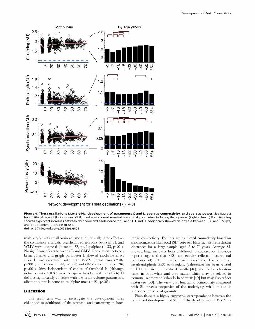
Figure 4. Theta oscillations (3.0–5.6 Hz) development of parameters C and L, average connectivity, and average power. See figure 2for additional legend. (Left column:) Childhood ages showed elevated levels of all parameters including theta power. (Right column:) Bootstrappingshowed significant increases between childhood and adolescence for C and SL. L and SL additionally showed an increase between ,30 and ,50 yrs,and a subsequent decrease to 55+.doi:10.1371/journal.pone.0036896.g004



reported in the extant literature. Peak levels of SL were found at

age ,50 for theta, alpha, and beta oscillations, while a significant

decrease in connectivity was found only in later life (55+). These

results are highly consistent with reported peak ages for WMV

development in large sample studies (peak at ,44 yrs for frontal

lobe WM [37], ,48 yrs for temporal lob [37]; 50.1 for whole brai

[33]; ,38 for whole brai [31]; ,43 for whole brai [32]; ,38 in

female WM [51]), although some reports could not establish

significant (nonlinear) trends in WMV development (in male [51])

or reported regional specificity in the peak age [37,52]. In

addition, WMV increases reflect ongoing myelination, which

shows a similarly protracted development (50–59 yr [53]).

Second, in a modestly sized subsample of young adults we

observed positive correlations between SL and MRI-derived

WMV for the oscillations across the three frequency bands (3.0–

25.0 Hz), which reached significance for the slower oscillation

networks (3.0–13.0 Hz). Although this result is limited to a single

age group of about 27 years, it suggests that SL may index

differences in adult WMV, the underlying developmental

processes of myelination leading up to adult WMV, and its

functional determinants or effect [54]. Given the importance of

oscillations in large-scale networks for cognitive processin [55], it

can be hypothesized that functional connectivity mediates this link

between WMV and cognition by increasing communication and

coordination between distant brain areas. In addition, our results

support the notion of EEG connectivity as a biomarker for

developmental psychopathology. For example, autism has been

related to both increased white matter and long range EEG

connectivit [54], whereas callosal white matter loss has been

related to decreased cross-hemispheric connectivity in Alzheimers’

diseas [56].

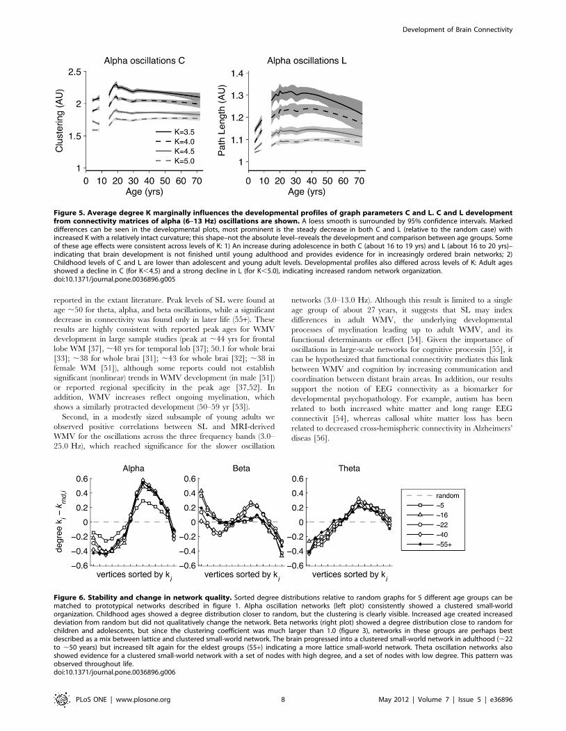
Figure 5. Average degree K marginally influences the developmental profiles of graph parameters C and L. C and L developmentfrom connectivity matrices of alpha (6–13 Hz) oscillations are shown. A loess smooth is surrounded by 95% confidence intervals. Markeddifferences can be seen in the developmental plots, most prominent is the steady decrease in both C and L (relative to the random case) withincreased K with a relatively intact curvature; this shape–not the absolute level–reveals the development and comparison between age groups. Someof these age effects were consistent across levels of K: 1) An increase during adolescence in both C (about 16 to 19 yrs) and L (about 16 to 20 yrs)–indicating that brain development is not finished until young adulthood and provides evidence for in increasingly ordered brain networks; 2)Childhood levels of C and L are lower than adolescent and young adult levels. Developmental profiles also differed across levels of K: Adult agesshowed a decline in C (for K,4.5) and a strong decline in L (for K,5.0), indicating increased random network organization.doi:10.1371/journal.pone.0036896.g005

Figure 6. Stability and change in network quality. Sorted degree distributions relative to random graphs for 5 different age groups can bematched to prototypical networks described in figure 1. Alpha oscillation networks (left plot) consistently showed a clustered small-worldorganization. Childhood ages showed a degree distribution closer to random, but the clustering is clearly visible. Increased age created increaseddeviation from random but did not qualitatively change the network. Beta networks (right plot) showed a degree distribution close to random forchildren and adolescents, but since the clustering coefficient was much larger than 1.0 (figure 3), networks in these groups are perhaps bestdescribed as a mix between lattice and clustered small-world network. The brain progressed into a clustered small-world network in adulthood (,22to ,50 years) but increased tilt again for the eldest groups (55+) indicating a more lattice small-world network. Theta oscillation networks alsoshowed evidence for a clustered small-world network with a set of nodes with high degree, and a set of nodes with low degree. This pattern wasobserved throughout life.doi:10.1371/journal.pone.0036896.g006



Besides average connectivity strength, we investigated the

pattern of connections using a graph theoretical approach. To

this end, we applied Watts and Strogatz’ [12] approach to estimate

C and L to the thresholded connectivity matrices. Contrary to

previous findings on the graph theoretical analysis of functional

connectivity networks (fMR [57], EE [58]), we found strong

increases in both C and L from childhood to adolescence as well as

within adolescence. This was found for all oscillations (3.0–

25.0 Hz). Concurrent increases in C and L are an indication of

decreased network randomness and increased orde [59,60].

Importantly, the developmental trend in the network parameters,

e.g. L in the alpha band, leveled off at a much earlier age than SL,

suggesting that it provides complementary information to SL on

the development of the brain network. The pattern of develop-

mental changes in network order was fairly independent of the

choice of threshold degree K. Across K levels, maximal values of C

and L were reached earlier (,18 yrs) than for SL. Although the

basic networks seem to be in place from a very early age

(Figure 6)[57,61–63], the increased order in the brain network

suggests that they nonetheless differ in randomness, and therefore

in essential computational capacities between childhood and

adolescenc [64]. This is consistent with the idea that maturation

reflects ongoing functional segregation of consistent networks that

are decreasingly diffus [63] and therefore less random.

A striking finding was that–in the theta band–the significant

decreases in connectivity in older age (55+) were accompanied by

decreases in L, suggesting that brain tissue atrophy results in

changes in the brain network. Decreases in L are hypothesized to

reflect efficiency in information transfe [10,15]. The neural loss

observed in later lif [65,66] may well be causative of this element

of reduced order in the brain network, and could perhaps be seen

as a non-clinical variant of the disrupted networks found in

Alzheimers’ Diseas [17,67].

Graph parameter L was positively correlated to WMV in an

adult sample. In addition, developmental profiles of both L and

WMV (as reported in the literature) show marked increases from

childhood to young adulthood. As with SL, these results suggest

that L is predictive of white matter development. This was

expected, since we have previously shown that L and SL are

correlated measure [68]. However, it was somewhat unexpected

that L (for alpha oscillation networks) positively correlated to

GMV. Thus, L carries additional information about functional

brain connectivity that is not covered by average connectivity

strength per se, but is reflected in the efficiency of the network

organization. The continuous decline of GMV in adolescence and

adult lif [30,37] is thought to reflect the degree of synaptic pruning

and connective trimmin [28,61,69]. The observed correlation

suggests that these pruning processes decrease network efficiency,

possibly by strengthening connectivity within subnetwork [63].

Note that it remains unclear how the positive correlation within

the young adult age group relates to the observed developmental

paths, so that firm conclusions cannot be drawn. Even so, the data

clearly suggest that L may be used to chart normal gray matter

development and psychopathology that is associated with abnor-

mal gray matter development, such as schizophrenia. Biomarkers

of schizophrenia include changes in the prefrontal cortex caused

by reduced neuropil (assumed to reflect loss of connectivity),

reduced spine densities, and smaller dendritic arbor [70,71], thus

resulting in GMV abnormalities. Indeed, graph theoretical

analysis of EEG and fMRI resting state activity has shown deviant

networks in this diseas [71,72].

The current results revealed increased connectivity for alpha

and beta band oscillations, but make no distinction between long

and short range connectivity. Short range connectivity requires

much denser electrode placement, which is likely to result in

spurious connectivity from volume conduction effect [73]. Recent

observations have suggested that the dichomotmy in projection

length is essential, and yields opposite results: decreased short

range connectivity concurs with increased long-range connectivity

with age. In an fMRI study it was shown that local activity in

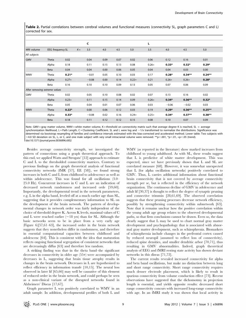
Table 2. Partial correlations between cerebral volumes and functional measures (connectivity SL, graph parameters C and L)corrected for sex.

C L

MRI volume EEG frequency SL K= 3.5 4.0 4.5 5.0 3.5 4.0 4.5 5.0

All subjects

GMV Theta 0.02 0.04 0.09 0.07 0.02 0.06 0.12 0.16 0.01

Alpha 0.18 0.11 0.15 0.13 0.08 0.26+ 0.33* 0.32* 0.29*

Beta 0.04 0.04 0.00 0.06 0.05 0.04 0.04 0.03 0.00

WMV Theta 0.21* 20.01 0.05 0.10 0.03 0.17 0.28* 0.34** 0.24**

Alpha 0.27+ 20.08 0.00 0.14 0.22+ 0.21 0.26+ 0.26+ 0.28*

Beta 0.16 0.10 0.10 0.09 0.13 0.05 0.07 0.06 0.09

After removing extreme values

GMV Theta 0.02 0.05 0.10 0.08 0.02 0.07 0.13 0.16 0.02

Alpha 0.23+ 0.11 0.15 0.14 0.09 0.26+ 0.34* 0.36** 0.32*

Beta 0.05 0.04 0.01 0.07 0.06 0.03 20.06 20.02 0.03

WMV Theta 0.22* 0.00 0.06 0.12 0.03 0.19 0.29* 0.36** 0.25**

Alpha 0.33* 20.08 0.02 0.16 0.24+ 0.25+ 0.34* 0.37** 0.38**

Beta 0.18 0.11 0.12 0.12 0.15 0.08 0.10 0.07 0.09

Note. GMV=gray matter volume, WMV=white matter volume, K = threshold on connectivity matrix such that average degree K is reached, SL = averagesynchronization likelihood, L = Path Length, C = Clustering Coefficient. SL and L were log and 21/x transformed to normalize the distributions. Significance wasdetermined via bootstrap resampling of families and confidence intervals estimated with the bias-corrected and accelerated method. Lower table: Two subjects with.4.0 SD deviation on SL, L, or C, and one male subject with very small intracranial volume were removed. **p,.001, *p,.01, +p,.05 (trend).doi:10.1371/journal.pone.0036896.t002



cognitive control networks becomes less diffuse with age, which is

accompanied by increased long distance functional connectivit

[74]. Similar findings of changes in (long-distance) connectivity

have been reporte [56,61,75]. The present results extend these

findings in showing that from childhood to adulthood brain

networks move from random to ordered. Since network param-

eters are relevant predictors of cognitive performanc [19,20], and

are disrupted in psychopathology [58], we can hypothesize that

the increased order is essential to the large developmental changes

in human cognitive performance during the same period. This

may be addressed in future investigations.

Topographical network quality–assessed by inspecting the

sorted degree distribution of the graphs and comparing these to

three prototypical network types (Lattice small-world, Clustered

small-world, and Scale-free)–showed evidence of clustered small-

world networks for many age groups and oscillation frequencies. A

clustered small-world network shows a group (or more than one

group) of hubs, consistent with a modular organization observed in

resting state fMR [76]. Similarly, evidence for clusters of hubs has

been presented in networks in both adults and infant [77]. The

current results showed that this network quality is relatively stable

over a wide age range (for alpha and theta oscillation networks),

but shows some development for networks derived from beta

frequency oscillations. The shift in tilt in the sorted degree

distribution for age groups ,5, ,16 and 55+ indicates that

younger age have an immature cluster of hubs that only becomes

fully operational at the age of ,22 years, and deterioration of that

cluster in older age.

In conclusion, we have shown that brain maturation across the

lifespan may be tracked using inexpensive EEG recordings. The

brain showed protracted increases in connectivity consistent with

white matter developmental curves, and changed from a relatively

random to a more ordered configuration. The EEG-derived

individual differences in connectivity and efficiency of the brain’s

connectivity network reflected actual anatomical differences as

assessed by MRI. Since the network parameters used here have

already been shown to be heritabl [21], they are prime candidates

to act as endophenotypes for establishing the connection between

genotype and brain function.

Author Contributions

Conceived and designed the experiments: DS HS DB HHP CS EdG.

Analyzed the data: DS MB HS. Contributed reagents/materials/analysis

tools: CS. Wrote the paper: DS MB SM HHP EdG.

References

1. Hagmann P, Cammoun L, Gigandet X, Meuli R, Honey CJ, et al. (2008)

Mapping the structural core of human cerebral cortex. PLoS Biol 6: e159.

doi:10.1371/journal.pbio.0060159.

2. Hagmann P, Sporns O, Madan N, Cammoun L, Pienaar R, et al. (2010) White

matter maturation reshapes structural connectivity in the late developing human

brain. Proceedings of the National Academy of Sciences 107: 19067–19072.

doi:10.1073/pnas.1009073107.

3. He Y, Chen ZJ, Evans AC (2007) Small-World Anatomical Networks in the

Human Brain Revealed by Cortical Thickness from MRI. Cereb Cortex 17:

2407–2419. doi:10.1093/cercor/bhl149.

4. Schmitt JE, Lenroot RK, Wallace GL, Ordaz S, Taylor KN, et al. (2008)

Identification of genetically mediated cortical networks: a multivariate study of

pediatric twins and siblings. Cereb Cortex 18: 1737–1747. doi:10.1093/cercor/

bhm211.

5. Raichle ME, MacLeod AM, Snyder AZ, Powers WJ, Gusnard DA, et al. (2001)

A default mode of brain function. Proceedings of the National Academy of

Sciences of the United States of America 98: 676–682.

6. Damoiseaux JS, Rombouts SARB, Barkhof F, Scheltens P, Stam CJ, et al. (2006)

Consistent resting-state networks across healthy subjects. Proceedings of the

National Academy of Sciences 103: 13848–13853. doi:10.1073/pnas.0601417103.

7. Britz J, Van De Ville D, Michel CM (2010) BOLD correlates of EEG

topography reveal rapid resting-state network dynamics. Neuroimage. Availa-

ble:http://www.ncbi.nlm.nih.gov/pubmed/20188188. Accessed: 2010 July 22.

8. Musso F, Brinkmeyer J, Mobascher A, Warbrick T, Winterer G (2010)

Spontaneous brain activity and EEG microstates. A novel EEG/fMRI analysis

approach to explore resting-state networks. Neuroimage. Available:http://www.

ncbi.nlm.nih.gov/pubmed/20139014. Accessed: 2010 July 22.

9. Bullmore E, Sporns O (2009) Complex brain networks: graph theoretical

analysis of structural and functional systems. Nat Rev Neurosci 10: 186–198.

doi:10.1038/nrn2575.

10. Latora V, Marchiori M (2003) Economic small-world behavior in weighted

networks. The European Physical Journal B 32: 15. doi:10.1140/epjb/e2003-

00095-5.

11. Newman MEJ (2003) The structure and function of complex networks. SIAM

review 45: 167.

12. Watts DJ, Strogatz SH (1998) Collective dynamics of /small-world/’ networks.

Nature 393: 440–442. doi:10.1038/30918.

13. Ponten SC, Bartolomei F, Stam CJ (2007) Small-world networks and epilepsy:

Graph theoretical analysis of intracerebrally recorded mesial temporal lobe

seizures. Clinical Neurophysiology 118: 918–927. doi:10.1016/

j.clinph.2006.12.002.

14. Stam CJ, de Haan W, Daffertshofer A, Jones B, Manshanden I, et al. (2009)

Graph theoretical analysis of magnetoencephalographic functional connectivity

in Alzheimer’s disease. Brain 132: 213–224. doi:10.1093/brain/awn262.

15. Achard S, Bullmore E (2007) Efficiency and cost of economical brain functional

networks. PLoS Comput Biol 3: e17. doi:10.1371/journal.pcbi.0030017.

16. Barahona M, Pecora LM (2002) Synchronization in Small-World Systems. Phys

Rev Lett 89: 054101. doi:10.1103/PhysRevLett.89.054101.

17. Stam CJ, Jones B, Nolte G, Breakspear M, Scheltens P (2007) Small-World

Networks and Functional Connectivity in Alzheimer’s Disease. Cereb Cortex 17:

92–99. doi:10.1093/cercor/bhj127.

18. Stam CJ (2004) Functional connectivity patterns of human magnetoencephalo-

graphic recordings: a ‘‘small-world’’ network? Neurosci Lett 355: 25–28.

19. Micheloyannis S, Pachou E, Stam CJ, Vourkas M, Erimaki S, et al. (2006) Using

graph theoretical analysis of multi channel EEG to evaluate the neural efficiency

hypothesis. Neurosci Lett 402: 273–277. doi:10.1016/j.neulet.2006.04.006.

20. van den Heuvel MP, Stam CJ, Kahn RS, Hulshoff Pol HE (2009) Efficiency of

functional brain networks and intellectual performance. J Neurosci 29:

7619–7624. doi:10.1523/JNEUROSCI.1443-09.2009.

21. Smit DJA, Stam CJ, Posthuma D, Boomsma DI, de Geus EJC (2008)

Heritability of ‘‘small-world’’ networks in the brain: a graph theoretical analysis

of resting-state EEG functional connectivity. Hum Brain Mapp 29: 1368–1378.

doi:10.1002/hbm.20468.

22. Fornito A, Zalesky A, Bassett DS, Meunier D, Ellison-Wright I, et al. (2011)

Genetic Influences on Cost-Efficient Organization of Human Cortical

Functional Networks. J Neurosci 31: 3261–3270. doi:10.1523/JNEUR-

OSCI.4858-10.2011.

23. de Haan, Pijnenburg YAL, Strijers RLM, van der Made Y, van der Flier WM,

et al. (2009) Functional neural network analysis in frontotemporal dementia and

Alzheimer’s disease using EEG and graph theory. BMC Neurosci 10: 101.

doi:10.1186/1471-2202-10-101.

24. He Y, Chen Z, Gong G, Evans A (2009) Neuronal networks in Alzheimer’s

disease. Neuroscientist 15: 333–350. doi:10.1177/1073858409334423.

25. Stam CJ (2010) Use of magnetoencephalography (MEG) to study functional

brain networks in neurodegenerative disorders. J Neurol Sci 289: 128–134.

doi:10.1016/j.jns.2009.08.028.

26. Amaral LA, Scala A, Barthelemy M, Stanley HE (2000) Classes of small-world

networks. Proceedings of the National Academy of Sciences of the United States

of America 97: 11149.

27. Bassett DS, Bullmore E (2006) Small-world brain networks. Neuroscientist 12:

512–523. doi:10.1177/1073858406293182.

28. Huttenlocher PR (1979) Synaptic density in human frontal cortex –

developmental changes and effects of aging. Brain Res 163: 195–205.

29. Courchesne E, Chisum HJ, Townsend J, Cowles A, Covington J, et al. (2000)

Normal Brain Development and Aging: Quantitative Analysis at in Vivo MR

Imaging in Healthy Volunteers1. Radiology 216: 672–682.

30. Gogtay N, Giedd JN, Lusk L, Hayashi KM, Greenstein D, et al. (2004) Dynamic

mapping of human cortical development during childhood through early

adulthood. Proc Natl Acad Sci 101: 8174–8179. doi:10.1073/pnas.0402680101.

31. Walhovd KB, Fjell AM, Reinvang I, Lundervold A, Dale AM, et al. (2005) Effects

of age on volumes of cortex, white matter and subcortical structures. Neurobiology

of Aging 26: 1261–1270. doi:10.1016/j.neurobiolaging.2005.05.020.

32. Walhovd KB, Fjell AM, Reinvang I, Lundervold A, Dale AM, et al. (2005)

Neuroanatomical aging: Universal but not uniform. Neurobiology of Aging 26:

1279–1282. doi:10.1016/j.neurobiolaging.2005.05.018.

33. Westlye LT, Walhovd KB, Dale AM, Bjørnerud A, Due-Tønnessen P, et al.

(2010) Life-Span Changes of the Human Brain White Matter: Diffusion Tensor



Imaging (DTI) and Volumetry. Cerebral Cortex 20: 2055–2068. doi:10.1093/cercor/bhp280.

34. Paus T (2010) Growth of white matter in the adolescent brain: Myelin or axon?Brain and cognition 72: 26–35.

35. Giedd, Blumenthal J, Jeffries NO, Castellanos FX, Liu H, et al. (1999) Braindevelopment during childhood and adolescence: a longitudinal MRI study. NatNeurosci 2: 861–863. doi:10.1038/13158.

36. Abe O, Yamasue H, Aoki S, Suga M, Yamada H, et al. (2008) Aging in theCNS: comparison of gray/white matter volume and diffusion tensor data.Neurobiology of Aging 29: 102–116.

37. Bartzokis G, Beckson M, Lu PH, Nuechterlein KH, Edwards N, et al. (2001)Age-Related Changes in Frontal and Temporal Lobe Volumes in Men: AMagnetic Resonance Imaging Study. Arch Gen Psychiatry 58: 461–465.doi:10.1001/archpsyc.58.5.461.

38. Pivik RT, Broughton RJ, Coppola R, Davidson RJ, Fox N, et al. (1993)Guidelines for the recording and quantitative analysis of electroencephalo-graphic activity in research contexts. Psychophysiology 30: 547–558.

39. Delorme A, Makeig (2004) EEGLAB: an open source toolbox for analysis ofsingle-trial EEG dynamics including independent component analysis. Journalof Neuroscience Methods 134: 9–21. doi:10.1016/j.jneumeth.2003.10.009.

40. Jung TP, Makeig S, Humphries C, Lee TW, Mckeown MJ, et al. (2000)Removing electroencephalographic artifacts by blind source separation.Psychophysiology 37: 163–178.

41. Stam CJ, van Dijk BW (2002) Synchronization likelihood: an unbiased measureof generalized synchronization in multivariate data sets. Physica D: NonlinearPhenomena 163: 236–251. doi:10.1016/S0167-2789(01)00386-4.

42. Montez, Poil S-S, Jones BF, Manshanden I, Verbunt JPA, et al. (2009) Alteredtemporal correlations in parietal alpha and prefrontal theta oscillations in early-stage Alzheimer disease. Proceedings of the National Academy of Sciences 106:1614–1619. doi:10.1073/pnas.0811699106.

43. Baare WFC, Hulshoff Pol HE, Boomsma DI, D. Posthuma, De Geus EJC, et al.(2001) Quantitative genetic modeling of variation in human brain morphology.Cerebral Cortex 11: 816–824.

44. Talairach J, Tournoux P (1988) Co-Planar Stereotaxic Atlas of the HumanBrain: 3-Dimensional Proportional System: An Approach to Cerebral Imaging.Thieme. 145 p.

45. Sled JG, Zijdenbos AP, Evans AC (1998) A nonparametric method forautomatic correction of intensity nonuniformity in MRI data. Medical Imaging,IEEE Transactions on 17: 87–97.

46. Schnack HG, Hulshoff Pol HE, Baare WFC, Staal WG, Viergever MA, et al.(2001) Automated Separation of Gray and White Matter from MR Images ofthe Human Brain. NeuroImage 13: 230–237. doi:10.1006/nimg.2000.0669.

47. DiCiccio TJ, Efron B (1996) Bootstrap confidence intervals. Statistical Science11: 189–228.

48. Teipel SJ, Pogarell O, Meindl T, Dietrich O, Sydykova D, et al. (2009) Regionalnetworks underlying interhemispheric connectivity: an EEG and DTI study inhealthy ageing and amnestic mild cognitive impairment. Human brain mapping30: 2098–2119.

49. Thatcher RW, Biver C, McAlaster R, Salazar A (1998) Biophysical Linkagebetween MRI and EEG Coherence in Closed Head Injury. Neuroimage 8:307–326.

50. Miot-Noirault E, Barantin L, Akoka S, Le Pape A (1997) T2 relaxation time as amarker of brain myelination: experimental MR study in two neonatal animalmodels. Journal of neuroscience methods 72: 5–14.

51. Good CD, Johnsrude IS, Ashburner J, Henson RNA, Fristen KJ, et al. (2002) Avoxel-based morphometric study of ageing in 465 normal adult human brains.Biomedical Imaging, 2002. 5th IEEE EMBS International Summer School on.16 p. doi:10.1109/SSBI.2002.1233974.

52. Allen JS, Bruss J, Brown CK, Damasio H (2005) Normal neuroanatomicalvariation due to age: the major lobes and a parcellation of the temporal region.Neurobiology of Aging 26: 1245–1260.

53. Benes FM, Turtle M, Khan Y, Farol P (1994) Myelination of a key relay zone inthe hippocampal formation occurs in the human brain during childhood,adolescence, and adulthood. Archives of General Psychiatry 51: 477.

54. Fields RD (2008) White matter in learning, cognition and psychiatric disorders.Trends in Neurosciences 31: 361–370. doi:10.1016/j.tins.2008.04.001.

55. Hipp JF, Engel AK, Siegel M (2011) Oscillatory Synchronization in Large-ScaleCortical Networks Predicts Perception. Neuron 69: 387–396. doi:10.1016/j.neuron.2010.12.027.

56. Pogarell O (2005) EEG coherence reflects regional corpus callosum area inAlzheimer’s disease. Journal of Neurology, Neurosurgery & Psychiatry 76:109–111. doi:10.1136/jnnp.2004.036566.

57. Supekar K, Musen M, Menon V (2009) Development of large-scale functionalbrain networks in children. PLoS Biol 7: e1000157. doi:10.1371/journal.-pbio.1000157.

58. Micheloyannis S, Vourkas M, Tsirka V, Karakonstantaki E, Kanatsouli K, et al.(2009) The influence of ageing on complex brain networks: a graph theoreticalanalysis. Hum Brain Mapp 30: 200–208. doi:10.1002/hbm.20492.

59. Stam CJ, de Haan W, Daffertshofer A, Jones BF, Manshanden I, et al. (2009)Graph theoretical analysis of magnetoencephalographic functional connectivityin Alzheimer’s disease. Brain 132: 213–224. doi:10.1093/brain/awn262.

61. Casey B, Trainor RJ, Orendi JL, Schubert AB, Nystrom LE, et al. (1997) Adevelopmental functional MRI study of prefrontal activation during perfor-mance of a go-no-go task. Journal of Cognitive Neuroscience 9: 835–847.

62. Fair DA, Cohen AL, Power JD, Dosenbach NUF, Church JA, et al. (2009)Functional Brain Networks Develop from a ‘‘Local to Distributed’’ Organiza-tion. PLoS Comput Biol 5: e1000381. doi:10.1371/journal.pcbi.1000381.

63. Jolles DD, van Buchem MA, Crone EA, Rombouts SARB (2011) AComprehensive Study of Whole-Brain Functional Connectivity in Childrenand Young Adults. Cerebral Cortex 21: 385–391. doi:10.1093/cercor/bhq104.

64. Achard S, Salvador R, Whitcher B, Suckling J, Bullmore E (2006) A resilient,low-frequency, small-world human brain functional network with highlyconnected association cortical hubs. J Neurosci 26: 63–72. doi:10.1523/JNEUROSCI.3874-05.2006.

65. Liu RSN, Lemieux L, Bell GS, Sisodiya SM, Shorvon SD, et al. (2003) Alongitudinal study of brain morphometrics using quantitative magneticresonance imaging and difference image analysis. NeuroImage 20: 22–33.doi:10.1016/S1053-8119(03)00219-2.

66. Raz N, Lindenberger U, Rodrigue KM, Kennedy KM, Head D, et al. (2005)Regional Brain Changes in Aging Healthy Adults: General Trends, IndividualDifferences and Modifiers. Cerebral Cortex 15: 1676–1689. doi:10.1093/cercor/bhi044.

67. Supekar K, Menon V, Rubin D, Musen M, Greicius MD (2008) NetworkAnalysis of Intrinsic Functional Brain Connectivity in Alzheimer’s Disease. PLoSComput Biol 4: doi:10.1371/journal.pcbi.1000100.

68. Smit DJA, Boersma M, Beijsterveldt CEM, Posthuma D, Boomsma DI, et al.(2010) Endophenotypes in a Dynamically Connected Brain. Behav Genet 40:167–177. doi:10.1007/s10519-009-9330-8.

69. Huttenlocher PR, de Courten C (1987) The development of synapses in striatecortex of man. Hum Neurobiol 6: 1–9.

70. McGlashan TH, Hoffman RE (2000) Schizophrenia as a Disorder ofDevelopmentally Reduced Synaptic Connectivity. Arch Gen Psychiatry 57:637–648. doi:10.1001/archpsyc.57.7.637.

71. Zipursky RB, Lim KO, Sullivan EV, Brown BW, Pfefferbaum A (1992)Widespread Cerebral Gray Matter Volume Deficits in Schizophrenia. Arch GenPsychiatry 49: 195–205.

72. Liu Y, Liang M, Zhou Y, He Y, Hao Y, et al. (2008) Disrupted small-worldnetworks in schizophrenia. Brain 131: 945–961. doi:10.1093/brain/awn018.

73. Micheloyannis S, Pachou E, Stam CJ, Breakspear M, Bitsios P, et al. (2006)Small-world networks and disturbed functional connectivity in schizophrenia.Schizophr Res 87: 60–66. doi:10.1016/j.schres.2006.06.028.

74. Nunez PL, Srinivasan R, Westdorp AF, Wijesinghe RS, Tucker DM, et al.(1997) EEG coherency: I: statistics, reference electrode, volume conduction,Laplacians, cortical imaging, and interpretation at multiple scales. Electroen-cephalography and Clinical Neurophysiology 103: 499–515. doi:10.1016/S0013-4694(97)00066-7.

75. Kelly A, Di Martino A, Uddin LQ, Shehzad Z, Gee DG, et al. (2009)Development of anterior cingulate functional connectivity from late childhood toearly adulthood. Cerebral Cortex 19: 640.

76. Dosenbach NUF, Nardos B, Cohen AL, Fair DA, Power JD, et al. (2010)Prediction of Individual Brain Maturity Using fMRI. Science 329: 1358–1361.doi:10.1126/science.1194144.

77. Meunier D, Achard S, Morcom A, Bullmore E (2009) Age-related changes inmodular organization of human brain functional networks. Neuroimage 44:715–723. doi:10.1016/j.neuroimage.2008.09.062.

78. Fransson P, Aden U, Blennow M, Lagercrantz H (2010) The FunctionalArchitecture of the Infant Brain as Revealed by Resting-State fMRI. CerebralCortex.



The brain matures with stronger functional connectivity and decreased randomness of its network

Documents

Transcript of The brain matures with stronger functional connectivity and decreased randomness of its network