A new procedure for monitoring the range and standard deviation of a quality characteristic

MPRAMunich Personal RePEc Archive

A new procedure for monitoring therange and standard deviation of a qualitycharacteristic

Mehdi Kiani and John Panaretos and Stelios Psarakis

2008

Online at http://mpra.ub.uni-muenchen.de/9067/MPRA Paper No. 9067, posted 11. June 2008 07:29 UTC

http://mpra.ub.uni-muenchen.de/

http://mpra.ub.uni-muenchen.de/9067/

Qual QuantDOI 10.1007/s11135-008-9175-x

ORIGINAL PAPER

A new procedure for monitoring the range and standarddeviation of a quality characteristic

M. Kiani · J. Panaretos · S. Psarakis

© Springer Science+Business Media B.V. 2008

Abstract The Shewhart and the Bonferroni-adjustment R and S chart are usually appliedto monitor the range and the standard deviation of a quality characteristic. These charts areused to recognize the process variability of a quality characteristic. The control limits ofthese charts are constructed on the assumption that the population follows approximately thenormal distribution with the standard deviation parameter known or unknown. In this article,we establish two new charts based approximately on the normal distribution. The constantvalues needed to construct the new control limits are dependent on the sample group size(k) and the sample subgroup size (n). Additionally, the unknown standard deviation forthe proposed approaches is estimated by a uniformly minimum variance unbiased estimator(UMVUE). This estimator has variance less than that of the estimator used in the Shewhart andBonferroni approach. The proposed approaches in the case of the unknown standarddeviation, give out-of-control average run length slightly less than the Shewhart approachand considerably less than the Bonferroni-adjustment approach.

Keywords Shewhart · Bonferroni-adjustment · Average run length · R chart · S chart

1 Introduction

The Shewhart and Bonferroni-adjustment control chart are common techniques for monitor-ing the process range and standard deviation of a quality characteristic. The Shewhart rangeand standard deviation control chart were introduced by Shewhart (1931). Ott (1975), Ryan(1989), Quesenberry (1997), Smith (1998) among others extended the Shewhart range andstandard deviation control charts. The Shewhart procedure usually is based on sample groupsizes (k) of at least 20–25 and on sample subgroup sizes (n) of at least 4–6. The Shewhart

M. Kiani · J. Panaretos (B) · S. PsarakisDepartment of Statistics, Athens University of Economics and Business, 76 Patision St,10434 Athens, Greecee-mail: [email protected]

123

M. Kiani et al.

chart with known and unknown standard deviation parameter is based on a random variablethat follows approximately the normal distribution.

In the case of the R chart, the values of the subgroup ranges (Ri ) are plotted on a chartthat includes the center line E(Ri ) and the following control limits

E(Ri )± Zα/2√

V ar(Ri ).

Here, the quality characteristics Xi j for i = 1, 2, . . . , k and j = 1, 2, . . . , n ( j th observationin i th subgroup) are supposed to be identically independently distributed according to thenormal distribution with mean µ and variance σ 2, and Ri = Xi(n) − Xi(1). Here, Xi(1) andXi(n) are order statistics of the random variable Xi j for the i th subgroup while E(Ri ) and√

V ar(Ri ) are the mean and standard deviation of Ri .It is well known (see e.g. Johnson, et al. 1994), that the joint probability density function

of Xi(1) and Xi(n) is given by

f1,n(x, y) ={

n(n − 1)[F(y)− F(x)]n−2 f (x) f (y), x < y0 x ≥ y.

Therefore, the joint probability density function of Xi(1) and R would be

f1,R(x, r) = n(n − 1)[F(r + x)− F(x)]n−2 f (x) f (r + x).

As a result, the probability density function of R is obtained to be

fR(r) =∫ +∞

−∞n(n − 1)[F(r + x)− F(x)]n−2 f (x) f (r + x)dx,

where the functions f (x) and F(x) are, respectively, the probability density function and thecumulative density function of the normal random variable X with parameters (µ, σ 2). Themean range (E(R)) can be evaluated to be

E(R) =∫ +∞

−∞

∫ +∞

−∞r × n(n − 1)[F(r + x)− F(x)]n−2 f (x) f (r + x)dxdr

=∫ +∞

−∞{1 − (F(x))n − (1 − F(x))n

}dx (1)

(see, e.g. Johnson et al. 1994).

Let Zi j = Xi j −µσ

i id∼ N (0, 1). Then the cumulative distribution function of Zi j = Z is

F(z) = 1√2π

∫ z

−∞e

−t22 dt, −∞ < z < +∞. (2)

Further, let R′ denote the range of order statistics Zh(1), Zh(2), . . . , Zh(n) for the hth subgroup(h = 1, 2, . . . , k). Then, using Eqs. 1 and 2, the mean of R′ is given by

E(R′) =∫ +∞

−∞

{1 −(

1√2π

∫ z

−∞e

−t22 dt

)n

−(

1 − 1√2π

∫ z

−∞e

−t22 dt

)n}dz.

The variance and the covariance of order statistics Zh(1), Zh(2), . . . Zh(n) can be extended as(see Johnson et al. 1994)

V ar(Zh(i)) = pi qi

n + 2{(F−1)′i }2 + pi qi

(n + 2)2{2(qi − pi )(F

−1)′i (F−1)′′i

+ pi qi {(F−1)′i (F−1)′′′i + 1

2

[(F−1)′′i

]2}}

+ · · · ,

123

A new procedure for monitoring the range and standard deviation of a quality characteristic

Cov(Zh(i), Zh( j)

) = pi q j

n + 2{(F−1)′i (F−1)′j } + pi qi

(n + 2)2

{(qi − pi )(F

−1)′′i (F−1)′j

+(q j − p j )(F−1)′′j (F−1)′i + 1

2pi qi (F

−1)′j (F−1)′′′i

+1

2p j q j (F

−1)′i (F−1)′′′j + 1

2pi q j (F

−1)′′i (F−1)′′j}

+ · · · ,

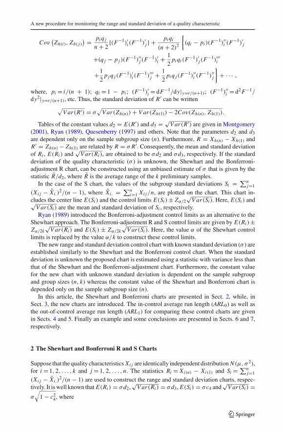
where, pi = i/(n + 1); qi = 1 − pi ; (F−1)′i = dF−1/dy|y=r/(n+1); (F−1)′′i = d2 F−1/

dy2|y=r/(n+1), etc. Thus, the standard deviation of R′ can be written√

V ar(R′) = σ√

V ar(Zh(n))+ V ar(Zh(1))− 2Cov(Zh(n), Zh(1)).

Tables of the constant values d2 = E(R′) and d3 = √V ar(R′) are given in Montgomery

(2001), Ryan (1989), Quesenberry (1997) and others. Note that the parameters d2 and d3

are dependent only on the sample subgroup size (n). Furthermore, R = Xh(n) − Xh(1) andR′ = Zh(n) − Zh(1) are related by R = σ R′. Consequently, the mean and standard deviationof Ri , E(Ri ) and

√V ar(Ri ), are obtained to be σd2 and σd3, respectively. If the standard

deviation of the quality characteristic (σ ) is unknown, the Shewhart and the Bonferroni-adjustment R chart, can be constructed using an unbiased estimate of σ that is given by thestatistic R/d2, where R is the average range of the k preliminary samples.

In the case of the S chart, the values of the subgroup standard deviations Si = ∑nj=1

(Xi j − Xi.)2/(n − 1), where Xi. = ∑n

i=1 Xi j/n, are plotted on the chart. This chart in-cludes the center line E(Si ) and the control limits E(Si )± Zα/2

√V ar(Si ). Here, E(Si ) and√

V ar(Si ) are the mean and standard deviation of Si , respectively.Ryan (1989) introduced the Bonferroni-adjustment control limits as an alternative to the

Shewhart approach. The Bonferroni-adjustment R and S control limits are given by E(Ri )±Zα/2k

√V ar(Ri ) and E(Si ) ± Zα/2k

√V ar(Si ). Here, the value α of the Shewhart control

limits is replaced by the value α/k to construct these control limits.The new range and standard deviation control chart with known standard deviation (σ ) are

established similarly to the Shewhart and the Bonferroni control chart. When the standarddeviation is unknown the proposed chart is estimated using a statistic with variance less thanthat of the Shewhart and the Bonferroni-adjustment chart. Furthermore, the constant valuefor the new chart with unknown standard deviation is dependent on the sample subgroupand group sizes (n, k) whereas the constant value of the Shewhart and Bonferroni chart isdepended only on the sample subgroup size (n).

In this article, the Shewhart and Bonferroni charts are presented in Sect. 2, while, inSect. 3, the new charts are introduced. The in-control average run length (ARL0) as well asthe out-of-control average run length (ARL1) for comparing these control charts are givenin Sects. 4 and 5. Finally an example and some conclusions are presented in Sects. 6 and 7,respectively.

2 The Shewhart and Bonferroni R and S Charts

Suppose that the quality characteristics Xi j are identically independent distribution N (µ, σ 2),for i = 1, 2, . . . , k and j = 1, 2, . . . , n. The statistics Ri = Xi(n) − Xi(1) and Si = ∑n

j=1

(Xi j − Xi.)2/(n − 1) are used to construct the range and standard deviation charts, respec-

tively. It is well known that E(Ri ) = σd2,√

V ar(Ri ) = σd3, E(Si ) = σc4 and√

V ar(Si ) =σ

√1 − c2

4, where

123

M. Kiani et al.

c4 =√

2

n − 1�[n

2

]/�

[(n − 1)

2

].

The Shewhart R chart with a known or unknown parameter σ are based on the randomvariables (Ri − E(Ri ))/

√V ar(Ri ) and (Ri − E(Ri ))/

√V ar(Ri ), respectively, and for the

Shewhart S chart, (Si − E(Si ))/√

V ar(Si ) and (Si − E(Si ))/√

V ar(Si ).

Let E(Ri ) = R,√

V ar(Ri ) = d3 R/d2, E(Si ) = S and√

V ar(Si ) = S√

1 − c24/c4,

where R = ∑ki=1 Ri/k and S = ∑k

i=1 Si/k. These variables, for sample sizes as large ask ≥ 20 and n ≥ 4, follow approximately the standard normal distribution.

The Shewhart R and S control limits for a known parameter σ , with confidence (1 −α)%,

are given by σ(d2 ± Zα/2d3) and σ(c4 ± Zα/2√

1 − c24), respectively. For these control limits,

the center line is σd2 and σc4, where the constant values d2, d3 and c4 depend only on thesample subgroup size (n).

If the standard deviation of the quality characteristic is unknown, then it is estimated bythe unbiased statistics R/d2 and S/c4 for Shewhart R and S chart, respectively. Then, thecenter line and the control limits for the Shewhart R chart with unknown parameter (σ ) takethe form

UCL = (R/d2)(d2 + zα/2d3); CL = R; LCL = (R/d2)(d2 − zα/2d3), (3)

while, for the Shewhart S chart,

UCL = (S/c4)(c4 + zα/2

√1 − c2

4); CL = S; LCL = (S/c4)(c4 − zα/2

√1 − c2

4). (4)

The Bonferroni-adjustment R and S control chart were suggested by Ryan (1989) in orderto improve the probability of detecting one or more false alarms of the Shewhart chart. TheBonferroni-adjustment R and S control limits for known standard deviation parameter aregiven below

σ(d2 ± Zα/2kd3); σ(c4 ± Zα/2k

√1 − c2

4). (5)

Furthermore, the Bonferroni R and S control limits with unknown parameter are

(R/d2)(d2 ± Zα/2kd3) (6)

(S/c4)(c4 − zα/2k

√1 − c2

4). (7)

The center lines for the Bonferroni R chart with known and unknown standard deviation areσd2 and R, respectively, and for the Bonferroni S chart, σc4 and S.

3 The New R and S chart

When the standard deviation is unknown, for constructing the new range and standard devi-ation charts, we need a good estimator of the standard deviation σ of the normal distributionN ∼ (µ, σ 2). A brief presentation of some estimators of the standard deviation is givenin Subsect. 3.1. A uniformly minimum variance unbiased (UMVU) estimator is suggestedin Sect. 3.2. The new R and S charts for both known and unknown standard deviation arepresented in Subsect. 3.3.

123


3.1 A Brief overview on the estimation of the standard deviation

Markowitz (1968) suggested the use of the minimum mean-square-error estimator of σ given

by σ =√∑n

i (Xi − X)2/k, where

k = 2

[�

(n + 1

2

)]2/[�(n

2

)]2.

Prescott (1971a) introduced a linear estimator for the standard deviation defined as σ = an W .Here, an is the unbiasing factor and W is given by

W =⎛

⎝n∑

j=n−r+1

Xi( j) −r∑

j=1

Xi( j)

⎞

⎠/(3r), i = 1, 2, . . . , k.

Furthermore, r = n/6 is rounded up to the nearest whole number if n/6 is not an integerand Xi(1) ≤ Xi(2) ≤ · · · ≤ Xi(n) is an ordered sample of the normal distribution N (µ, σ 2).Prescott (1971b) proposed the use of another estimator for the standard deviation of theN (µ, σ 2) given by

σ =n∑

j=1

m j Xi( j)

/ n∑

j=1

m2j .

In this case, m j = E((Xi( j) − µ)/σ

).

Healy (1978) introduced the unbiased estimator of σ given by

σ = √π

n∑

i=1

(2i − n − 1)Xi/{n(n − 1/2)}.

Vardeman (1999) considered using minimum mean-square-error estimator given, for thecase of a single sample, by

σ = Rd2

d22 + d2

3

; σ = S

c4,

where R and S are the range and standard deviation of the single sample, and the constantsd2, d3 and c4 are as introduced in previous sections. He also introduced a combination ofseveral estimators for the case of r samples of possibly different sizes n1, n2, . . . , nr withranges R1, R2, . . . , Rr defined by σ = γ1 R1 + γ2 R2 + · · · + γr Rr , where

γi =(

r∑

i=1

d22 (ni )

d23 (ni )

)−1d2(ni )

d23 (ni )

; d2(ni ) = E(Ri )/σ ; d3(ni ) = √V ar(Ri )/σ.

An analogous estimator was proposed for the case of r samples of possibly different sizesn1, n2, . . . , nr with sample standard deviation estimators S1, S2, . . . , Sr . The proposed esti-mators are σ = γ1S1 + γ2S2 + · · · + γr Sr and σ = Spooled/c4(v + 1). Here,

γi =(

r∑

i=1

c24(ni )

c25(ni )

)−1c4(ni )

c25(ni )

; c4(ni ) = E(Si )/σ ; c5(ni ) = √V ar(Si )/σ

123

M. Kiani et al.

S2pooled = (n1 − 1)S2

1 + (n2 − 1)S22 + · · · + (nr − 1)S2

r

(n1 − 1)+ (n2 − 1)+ · · · + (nr − 1);

v = (n1 − 1)+ (n2 − 1)+ · · · + (nr − 1).

Some other estimators of the standard deviation have also been given by Glasser (1962), Khan(1968), Gurland and Tripathi (1971), Donatos (1989), Arnholt and Hebert (1995), Watson(1997). However, these authors did not employ UMVU estimators of the standard deviationof the normal distribution N (µ, σ 2).

3.2 An UMVU estimator of the standard deviation

As is well known, the random variable k(n − 1)S2/σ 2 is chi-square distributed. Let

S =√√√√

k∑

i=1

n∑

j=1

(Xi j − Xi.)2/ (k(n − 1)).

Then, the random variable H = √k(n − 1)S/σ follows the chi distribution with k(n − 1)

degrees of freedom. The probability density function and the r th raw moment of H are

PH (h) = 1

2(k(n−1)/2)−1� (k(n − 1)/2)e−h2/2hk(n−1)−1, h > 0 (8)

E(Hr ) =√

2r� ((k(n − 1)+ r)/2)

� (k(n − 1)/2). (9)

Moreover, the standard chi distribution (8) is in fact a standard gamma distribution withprobability density function

PH (h) = 1

ηζ� (ζ )e−(h−γ )/η(h − γ )ζ−1, h > 0,

where, the values ζ , η, and γ are k(n − 1)/2, 2, and 0, respectively, with H replacingH2. Assume further a constant value ψ to be the unbiasing factor of the standard deviationestimator, where

ψ =(√

2k(n−1)�

(k(n−1)+1

2

)/�(

k(n−1)2

)), kn < 350

and

ψ ≈ 4k(n − 1)

4k(n − 1)+ 1, kn ≥ 350

The mean and variance of the statistic S are evaluated to be σψ and σ 2(1−ψ2), respectively,using Eq. 9. Thus, the statistic S/ψ is an unbiased estimator of the standard deviation (σ ). Inthis case, the constant value ψ depends on both the sample subgroup size (n) and the samplegroup size (k). The value of ψ with various sample sizes k and n is given in appendix CTable 10, for

k = 2(1)10, 15(5)30, 40, 100, 120

and

n = 2(1)11, 14, 15, 18, 20(5)50, 60(10)120.

123


Table 1 The variance of the statisticsS/ψ , R/d2 and S/c4 with σ 2 = 1

k

n 2 5 10 15 20 25 60 120

σ 2(

1 − ψ2)/ψ2 2 0.27323 0.10440 0.05118 0.03392 0.02527 0.02015 0.00838 0.00413

5 0.06427 0.02527 0.01267 0.00838 0.00620 0.00499 0.00209 0.00104

10 0.02819 0.01117 0.00557 0.00374 0.00280 0.00228 0.00093 0.00046

20 0.01328 0.00531 0.00277 0.00172 0.00132 0.00105 0.00044 0.00022

25 0.01048 0.00413 0.00209 0.00139 0.00104 0.00083 0.00035 0.00017

σ 2d23/(

kd22

)2 0.28592 0.11437 0.05718 0.03812 0.02859 0.02287 0.00953 0.00477

5 0.06899 0.02760 0.01380 0.00920 0.00690 0.00552 0.00230 0.00115

10 0.03352 0.01341 0.00670 0.00447 0.00335 0.00268 0.00112 0.00056

20 0.01905 0.00762 0.00381 0.00254 0.00190 0.00152 0.00063 0.00032

25 0.01622 0.00649 0.00324 0.00216 0.00162 0.00130 0.00054 0.00027

σ 2(

1 − c24

)/(kc2

4

)2 0.28537 0.11415 0.05707 0.03805 0.02854 0.02283 0.00951 0.00476

5 0.06587 0.02635 0.01317 0.00878 0.00659 0.00527 0.00220 0.00110

10 0.02846 0.01138 0.00569 0.00379 0.00285 0.00228 0.00095 0.00047

20 0.01336 0.00534 0.00267 0.00178 0.00134 0.00107 0.00045 0.00022

25 0.01056 0.00423 0.00211 0.00141 0.00106 0.00085 0.00035 0.00018

The statistic S is an injective function of the complete sufficient statistic S2 and the statisticS/ψ is an unbiased estimator of σ . Therefore according to the Lehman-Scheffe theorem, thestatistic S/ψ is an UMVU estimator of σ (see Rohatgi 1984). Then, the UMVU estimatorS/ψ can be used for constructing the new range and standard deviation control chart withunknown standard deviation. In the sequel, we compare the range and standard deviation con-trol charts that are based on the statistic R/d2 (for the Shewhart and Bonferroni approach) tothose based on the statistic S/ψ (for the new approach). Table 1 shows that the variance ofthe statistic S/ψ , var(S/ψ) = σ 2(1 − ψ2)/ψ2, is less than that of the statistics R/d2 andS/c4, i.e., var(R/d2) = σ 2d2

3/(kd22 ) and var(S/c4) = σ 2(1 − c2

4)/(kc24).

3.3 The New R and S charts

The control limits for the average of a quality characteristic depend on the variability of theproduction process. While the process variability is outside the control limits, the controllimits on the average quality characteristic will not have much meaning. Therefore, it is bestthat a range or standard deviation control limits is first set (see Montgomery 2001).

The quality characteristics Xi j for i = 1, 2, . . . , k and j = 1, 2, . . . , n are identicallyand independently normally distributed with mean µ and variance σ 2. The new range andstandard deviation control charts with known standard deviation, like the Shewhart R and Scontrol charts, are given by

UCL = σ(d2 + zα/2d3); C L = σd2; LCL = σ(d2 − zα/2d3)

UCL = σ

(c4 + Zα/2

√1 − c2

4

); C L = σc4; LCL = σ

(c4 − Zα/2

√1 − c2

4

).

To establish the proposed control charts with unknown standard deviation, we estimate

E(Ri ) = σd2,√

V ar(Ri ) = σd3, E(Si ) = σc4 and√

V ar(Si ) = σ

√1 − c2

4 using the

123

M. Kiani et al.

UMVU estimators Sd2/ψ , Sd3/ψ , Sc4/ψ and S√

1 − c24/ψ , respectively. The resulting

control limits for the proposed R chart with unknown standard deviation would be

UCL = (S/ψ)(d2 + zα/2d3); CL = (S/ψ)(d2); LCL = (S/ψ)(d2 − zα/2d3) (10)

and the control limits for the proposed S chart are

UCL = (S/ψ)

(c4+zα/2

√1−c2

4

); CL = Sc4/ψ; LCL = (S/ψ)

(c4−zα/2

√1−c2

4

).

(11)

In Sects. 4 and 5, the in-control and out-of-control average run length for the Shewhart,Bonferroni and new R and S control charts are examined.

4 In-control average run length

The in-control average run length (called ARL0) is the average number of subgroup rangesor standard deviations that should be plotted before a subgroup range or standard deviationindicates an out-of-control condition. The ARL0 can be calculated from ARL0 = 1/p underthe condition that the process observations are uncorrelated. Here, p is the probability thatany point exceeds the control limits. The in-control average run length can be used to evaluatethe performance of the control chart.

In this section, the average run length is considered for the initial group and groups2, 3, . . . with known and unknown parameter σ when the process is in control. Let the indi-vidual events Gi denote the subgroup range Ri or standard deviation Si exceeds the controllimits of the in control process (R = R0 or σ = σ0).

For the initial group of observations with unknown parameter σ , the events Gi and Gi ′for i �= i ′ = 1, 2, . . . , k are not independent, since the statistics Ri − UCL and R j − UCL ,or Si − UCL and S j − UCL , for the Shewhart, the Bonferroni and the new charts are basedon the same observations of the initial group.

In case the events Gi are independent, the sequence of trials, comparing Ri with UCL orSi with UCL will be a sequence of Bernoulli trials and the run length between occurrencesof Gi will be a Geometric random variable with probability α = P(Gi ). Additionally, thein-control average run length would be 1/P(Gi ) or 1/α such that,

P(Gi ) = P(Ri ≤ LCL or Ri ≥ UCL |R = R0 ) (12)

or

P(Gi ) = P(Si ≤ LCL or Si ≥ UCL |σ = σ0 ). (13)

However, the statistics Ri − UCL and R j − UCL or Si − UCL and S j − UCL for the initialgroup with unknown parameter are not independent events. Therefore, the in-control ARLfor the initial group with unknown parameter can be not calculated.

For the initial group with known parameter, the correlation between random variablesRi −UCL and R j −UCL or Si −UCL and S j −UCL can be obtained to be 0. Here, the UCLwith known parameter is a constant value and the subgroup ranges Ri and R j or standarddeviations Si and S j are independent. Thus, the events Gi and G j for the initial group withknown parameter are uncorrelated.

123


For the groups 2, 3, . . . with known and unknown parameter, the events Gi and G j areuncorrelated, since the UCL with known and unknown parameter are based on the obser-vations of initial group, while the Ri or Si belong to groups 2, 3, . . . . Thus, the correlationbetween random variables Ri − UCL and R j − UCL or Si − UCL and S j − UCL can beobtained to be 0.

Based on the above, the sequence of the events {Gi }, for the initial group with knownparameter and the groups 2, 3, . . . with known and unknown parameter, would be Bernoullitrials and the run length between occurrences of Gi would be a Geometric random variablewith probability P(Gi ). The probability P(Gi ) for both the Shewhart and the new approachis α, and for the Bonferroni-adjustment approach is α/k. As a result, the in-control averagerun length (ARL0) would be 1/P(Gi ) = 1/α for the Shewhart and the new approach, and1/P(Gi ) = k/α for the Bonferroni-adjustment approach. Thus the ARL0 for the Shewhartand proposed chart (1/α) is less than the ARL0 for Bonferroni-adjustment chart (k/α, fork ≥ 2). (See, also, Nedumaran and Pignatiello 2005, Tsai et al. 2005).

Now, we discuss the in-control average run length that based on the average number ofgroups before a group indicates an out-of-control condition. Here, the in-control average runlength is called ARL ′

0.For the initial group with known parameter and the groups 2, 3, . . . with known and

unknown parameter, let the random variable Y denote the overall occurrences of events Gi

for i = 1, 2, . . . , k. Then, this random variable should follow the Binomial distribution withprobability distribution (for the Shewhart and the new approach) given by

P(Y = y) =(

ky

)αy(1 − α)k−y, y = 0, 1, 2, . . . , k.

Therefore, the probability of one or more subgroup ranges or standard deviation falling outof the control limits (the probability of out-of-control condition for a group) for the Shewhartand the new approach is P(Y ≥ 1) = 1 − (1 −α)k . Ryan (1989) showed that the probability1 − (1 − α)k is approximately equal with kα. Thus, Ryan (1989) suggested the Bonferroni-adjustment approach for the control limits. In this case, the probability of one or more falsealarm is improved to 1 − (1 − α/k)k that is less than 1 − (1 − α)k . The probability distri-bution of Y , for the Bonferroni-adjustment approach, follows the Binomial distribution withparameters (k, α/k). Therefore, the probability of one or more subgroup ranges or standarddeviations falling out of the control limits for the Bonferroni-adjustment approach is givenby P(Y ≥ 1) = 1− (1−α/k)k . As a result, the ARL ′

0 is obtained to be 1/(1− (1−α)k) forthe Shewhart and the new approach, and 1/(1 − (1 − α/k)k) for the Bonferroni-adjustmentapproach. That means 1/(1−(1−α)k) < 1/(1−(1−α/k)k . Thus, the ARL ′

0 for the Shewhartand the new approach is less than that of the Bonferroni-adjustment approach. Consequently,the in-control average run length (ARL0, ARL ′

0) for the Bonferroni-adjustment approach isgreater than the Shewhart and the new approach. In the next section, we illustrate that theout-of-control average run length for the Bonferroni-adjustment approach is not so satisfac-tory. In other words, the power of the Bonferroni-adjustment control limits is considerablyless than the one of the Shewhart and new approach.

5 Out-of-control average run length

The ability of the range and standard deviation control charts to detect shifts in processquality is described by the out-of-control average run length (ARL1). The probabilities ofdetecting a one or more false alarms when the process is in control were improved by using

123

M. Kiani et al.

the Bonferroni-adjustment approach. In this section, the power of control limits for the usualapproach (Shewhart and Bonferroni) and the new approach are compared using ARL1.

If the in-control value of the standard deviation shifts from σ0 to σ1 = λσ0 > σ0, (λ > 1)the probability of not detecting the range or standard deviation shift (β) is calculated by

β = P (LCL ≤ Ri ≤ UCL |σ = λσ0 ) (R Chart) (14)

or

β = P (LCL ≤ Si ≤ UCL |σ = λσ0 ) (S Chart). (15)

These probabilities for both the Shewhart and proposed R and S charts with known parameter(σ ) similarly are obtained to be

β = P

(−Zα/2d3 + d2(1 − λ)

λd3≤ Zi ≤ Zα/2d3 + d2(1 − λ)

λd3

)(R Chart) (16)

and

β = P

⎛

⎝−Zα/2

√1 − c2

4 + c4(1 − λ)

λ

√1 − c2

4

≤ Zi ≤Zα/2√

1 − c24 + c4(1 − λ)

λ

√1 − c2

4

⎞

⎠ (S Chart).

(17)

Meanwhile, the probability β for the Bonferroni-adjustment R and S chart with knownparameter (σ ) is

β = P

(−Zα/2kd3 + d2(1 − λ)

λd3≤ Zi ≤ Zα/2kd3 + d2(1 − λ)

λd3

)(R Chart) (18)

and

β = P

⎛

⎝−Zα/2k

√1 − c2

4 + c4(1 − λ)

λ

√1 − c2

4

≤ Zi ≤Zα/2k

√1 − c2

4 + c4(1 − λ)

λ

√1 − c2

4

⎞

⎠ (S Chart).

(19)

Usually, the parameter σ is unknown. In this case, we obtain the probability β for the controllimits with unknown parameter. We already showed that S/ψ is a UMVU estimator of thestandard deviation. Let us call S/ψ by St . In order to compute the type II error (β) for theShewhart, the Bonferroni and the proposed approach with unknown parameter the standarddeviation (σ0) from Eqs. 14 and 15 is estimated by St . Thus, the probabilityβ for the Shewhartapproach with unknown parameter is calculated using Eqs. 3 and 14 for R chart and Eqs. 4and 15 for S chart

β = P

((R/d2)(d2 − Zα/2d3)− λSt d2

λSt d3≤ Zi ≤ (R/d2)(d2 + Zα/2d3)− λSt d2

λSt d3

)

(20)

and

β=P

⎛

⎝(S/c4)(c4−Zα/2

√1−c2

4)−λSt c4

λSt

√1−c2

4

≤ Zi ≤(S/c4)(c4+Zα/2

√1−c2

4)−λSt c4

λSt

√1−c2

4

⎞

⎠ .

(21)

123


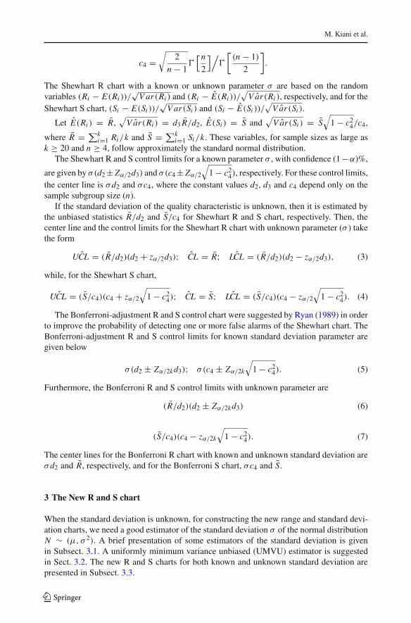
Table 2 The constant values d2, d3 and c4 to construct the OC curves

n

2 5 10 20 25

d2 1.128 2.326 3.078 3.735 3.931

d3 0.853 0.864 0.797 0.729 0.708

c4 0.7979 0.9400 0.9727 0.9869 0.9896

Similarly, the probability β for the Bonferroni-adjustment approach with unknown parameteris obtained by using Eqs. 6 and 14 for R chart and Eqs. 7 and 15 for S chart,

β = P

((R/d2)(d2 − Zα/2kd3)− λSt d2

λSt d3≤ Zi ≤ (R/d2)(d2 + Zα/2kd3/d2)− λSt d2

λSt d3

)

(22)

and

β=P

⎛

⎝(S/c4)(c4−Zα/2k

√1−c2

4)−λSt c4

λSt

√1−c2

4

≤ Zi ≤(S/c4)(c4+Zα/2k

√1−c2

4)−λSt c4

λSt

√1−c2

4

⎞

⎠ .

(23)

Also, the probability β for the new approach with unknown parameter is obtained usingEqs. 10 and 14 for R chart and Eqs. 11 and 15 for S chart as follow

β = P

((S/ψ)(d2 − Zα/2d3)− λSt d2

λSt d3≤ Zi ≤ (S/ψ)(d2 + Zα/2d3)− λSt d2

λSt d3

)(24)

and

β=P

⎛

⎝(S/ψ)(c4−Zα/2

√1−c2

4)−λSt c4

λSt

√1−c2

4

≤ Zi ≤(S/ψ)(c4+Zα/2

√1−c2

4)−λSt c4

λSt

√1−c2

4

⎞

⎠ .

(25)

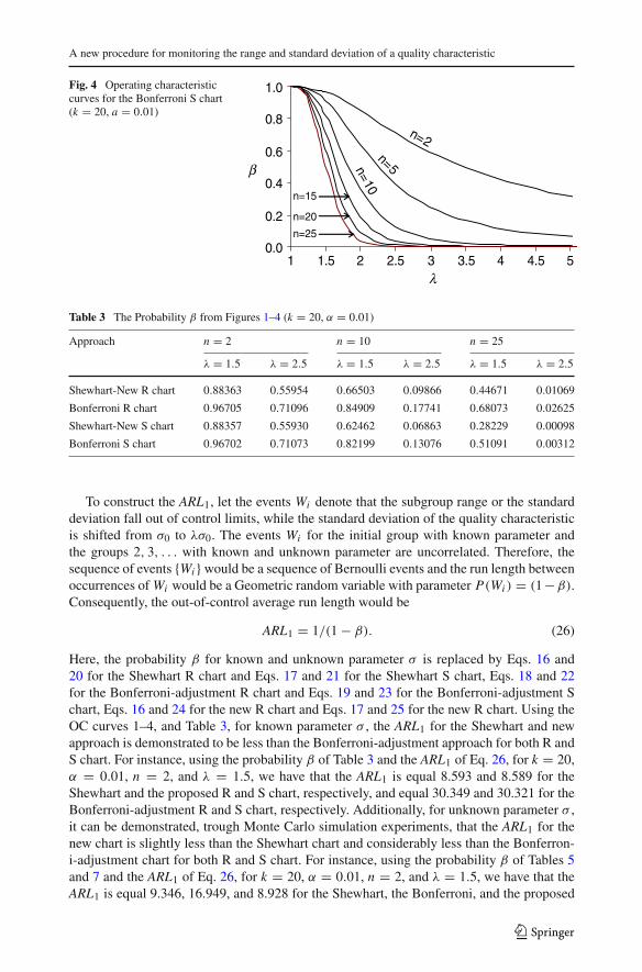
The probability β with known standard deviation for various sample sizes n and coefficientλ is exhibited by the operating-characteristic (OC) curves. The OC curves are constructedaccording to the constant values of Table 2 and Eqs. 16 and 17 for the Shewhart and the newR and S charts, respectively, and Eqs. 18 and 19 for the Bonferroni-adjustment R and S chart.

Figures 1–4 indicate that the Shewhart and the new approach are considerably effectivein detecting shifts greater than one standard deviation (λ> 1) on the first sample followingthe shift. Table 3 shows the probability β for various shifts and sample sizes from Figs. 1–4.This table indicates that the probability β for the Shewhart and the new approach is less thanthe probability in not detecting a shift for the Bonferroni-adjustment approach.

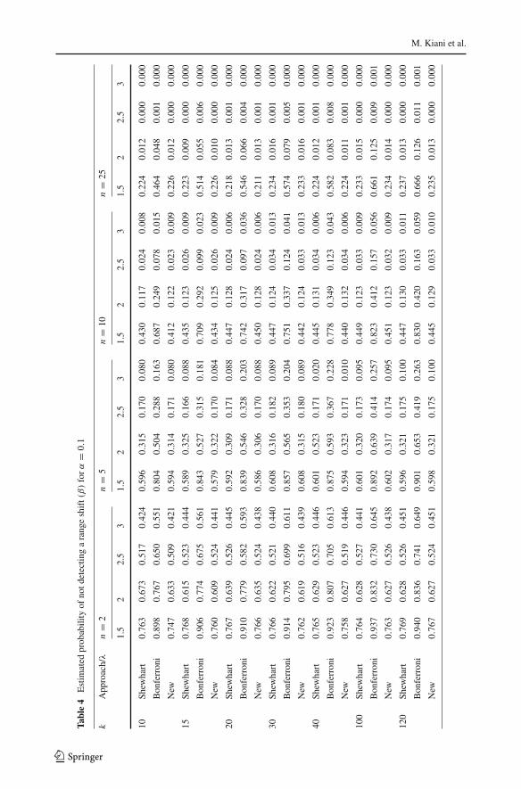
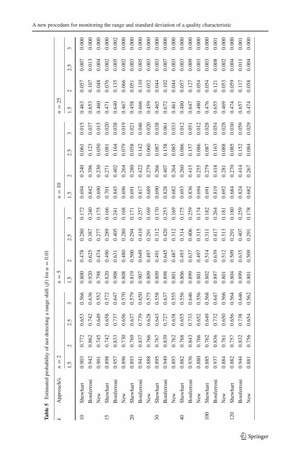
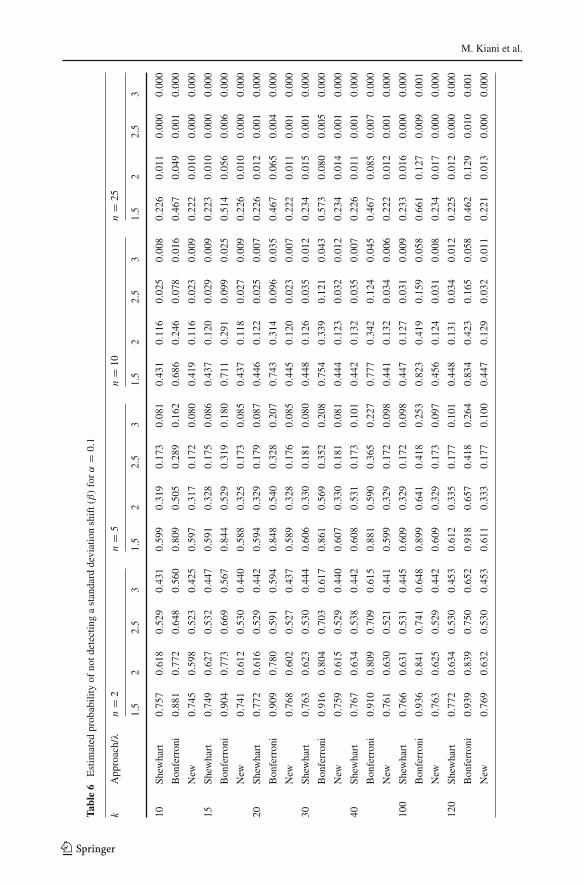
The probability β with unknown standard deviation for various sample sizes n and k, andcoefficient λ is exhibited by Tables 4 and 5 for R chart, and Tables 6 and 7 for S chart. Thesetables are constructed using Monte Carlo simulation experiments (Appendix A for R chartand Appendix B for S chart) with constant values of Table 2 and Eqs. 20, 22, and 24 forthe Shewhart, the Bonferroni-adjustment, and the new R chart, respectively, and Eqs. 21, 23,

123

M. Kiani et al.

Fig. 1 Operating characteristiccurves for the Shewhart and newR chart (k = 20, a = 0.01)

n=2

n=5n=10

n=15

n=20

n=25

0.0

0.2

0.4

0.6

0.8

1.0

1 1.5 2 2.5 3 3.5 4 4.5 5

β

λ

Fig. 2 Operating characteristiccurves for the Bonferroni R chart(k = 20, a = 0.01) n=2

n=5n=10

n=15n=20n=25

0.0

0.2

0.4

0.6

0.8

1.0

1 1.5 2 2.5 3 3.5 4 4.5 5

β

λ

Fig. 3 Operating characteristiccurves for the Shewhart and newS chart (k = 20, a = 0.01)

n=2

n=5n=10

n=15

n=20

n=250.0

0.2

0.4

0.6

0.8

1.0

1 1.5 2 2.5 3 3.5 4 4.5 5

β

λ

and 25 for the Shewhart, the Bonferroni-adjustment, and the new S chart, respectively. If thesubgroup range or standard deviation falls out of the control limits, a counter for that wasincreased by one. This procedure was replicated 10,000 times, and then the probability β wasestimated by dividing the number of replications in which points exceeded the control limitswith the total number of replications. As a result, the estimated probability of not detecting arange or a standard deviation shift for the Shewhart, the Bonferroni-adjustment and the newR and S chart are shown in the following Tables 4–7.

The results in Tables 4–7 show that with unknown standard deviation the new R and Schart perform better than both the Shewhart and the Bonferroni-adjustment R and S chart.

123


Fig. 4 Operating characteristiccurves for the Bonferroni S chart(k = 20, a = 0.01)

n=2n=5n=10

n=15

n=20

n=250.0

0.2

0.4

0.6

0.8

1.0

1 1.5 2 2.5 3 3.5 4 4.5 5

β

λ

Table 3 The Probability β from Figures 1–4 (k = 20, α = 0.01)

Approach n = 2 n = 10 n = 25

λ = 1.5 λ = 2.5 λ = 1.5 λ = 2.5 λ = 1.5 λ = 2.5

Shewhart-New R chart 0.88363 0.55954 0.66503 0.09866 0.44671 0.01069

Bonferroni R chart 0.96705 0.71096 0.84909 0.17741 0.68073 0.02625

Shewhart-New S chart 0.88357 0.55930 0.62462 0.06863 0.28229 0.00098

Bonferroni S chart 0.96702 0.71073 0.82199 0.13076 0.51091 0.00312

To construct the ARL1, let the events Wi denote that the subgroup range or the standarddeviation fall out of control limits, while the standard deviation of the quality characteristicis shifted from σ0 to λσ0. The events Wi for the initial group with known parameter andthe groups 2, 3, . . . with known and unknown parameter are uncorrelated. Therefore, thesequence of events {Wi } would be a sequence of Bernoulli events and the run length betweenoccurrences of Wi would be a Geometric random variable with parameter P(Wi ) = (1 −β).Consequently, the out-of-control average run length would be

ARL1 = 1/(1 − β). (26)

Here, the probability β for known and unknown parameter σ is replaced by Eqs. 16 and20 for the Shewhart R chart and Eqs. 17 and 21 for the Shewhart S chart, Eqs. 18 and 22for the Bonferroni-adjustment R chart and Eqs. 19 and 23 for the Bonferroni-adjustment Schart, Eqs. 16 and 24 for the new R chart and Eqs. 17 and 25 for the new R chart. Using theOC curves 1–4, and Table 3, for known parameter σ , the ARL1 for the Shewhart and newapproach is demonstrated to be less than the Bonferroni-adjustment approach for both R andS chart. For instance, using the probability β of Table 3 and the ARL1 of Eq. 26, for k = 20,α = 0.01, n = 2, and λ = 1.5, we have that the ARL1 is equal 8.593 and 8.589 for theShewhart and the proposed R and S chart, respectively, and equal 30.349 and 30.321 for theBonferroni-adjustment R and S chart, respectively. Additionally, for unknown parameter σ ,it can be demonstrated, trough Monte Carlo simulation experiments, that the ARL1 for thenew chart is slightly less than the Shewhart chart and considerably less than the Bonferron-i-adjustment chart for both R and S chart. For instance, using the probability β of Tables 5and 7 and the ARL1 of Eq. 26, for k = 20, α = 0.01, n = 2, and λ = 1.5, we have that theARL1 is equal 9.346, 16.949, and 8.928 for the Shewhart, the Bonferroni, and the proposed

123

M. Kiani et al.

Tabl

e4

Est

imat

edpr

obab

ility

ofno

tdet

ectin

ga

rang

esh

ift(β)

forα

=0.

1

kA

ppro

ach/λ

n=

2n

=5

n=

10n

=25

1.5

22.

53

1.5

22.

53

1.5

22.

53

1.5

22.

53

10Sh

ewha

rt0.

763

0.67

30.

517

0.42

40.

596

0.31

50.

170

0.08

00.

430

0.11

70.

024

0.00

80.

224

0.01

20.

000

0.00

0

Bon

ferr

oni

0.89

80.

767

0.65

00.

551

0.80

40.

504

0.28

80.

163

0.68

70.

249

0.07

80.

015

0.46

40.

048

0.00

10.

000

New

0.74

70.

633

0.50

90.

421

0.59

40.

314

0.17

10.

080

0.41

20.

122

0.02

30.

009

0.22

60.

012

0.00

00.

000

15Sh

ewha

rt0.

768

0.61

50.

523

0.44

40.

589

0.32

50.

166

0.08

80.

435

0.12

30.

026

0.00

90.

223

0.00

90.

000

0.00

0

Bon

ferr

oni

0.90

60.

774

0.67

50.

561

0.84

30.

527

0.31

50.

181

0.70

90.

292

0.09

90.

023

0.51

40.

055

0.00

60.

000

New

0.76

00.

609

0.52

40.

441

0.57

90.

322

0.17

00.

084

0.43

40.

125

0.02

60.

009

0.22

60.

010

0.00

00.

000

20Sh

ewha

rt0.

767

0.63

90.

526

0.44

50.

592

0.30

90.

171

0.08

80.

447

0.12

80.

024

0.00

60.

218

0.01

30.

001

0.00

0

Bon

ferr

oni

0.91

00.

779

0.58

20.

593

0.83

90.

546

0.32

80.

203

0.74

20.

317

0.09

70.

036

0.54

60.

066

0.00

40.

000

New

0.76

60.

635

0.52

40.

438

0.58

60.

306

0.17

00.

088

0.45

00.

128

0.02

40.

006

0.21

10.

013

0.00

10.

000

30Sh

ewha

rt0.

766

0.62

20.

521

0.44

00.

608

0.31

60.

182

0.08

90.

447

0.12

40.

034

0.01

30.

234

0.01

60.

001

0.00

0

Bon

ferr

oni

0.91

40.

795

0.69

90.

611

0.85

70.

565

0.35

30.

204

0.75

10.

337

0.12

40.

041

0.57

40.

079

0.00

50.

000

New

0.76

20.

619

0.51

60.

439

0.60

80.

315

0.18

00.

089

0.44

20.

124

0.03

30.

013

0.23

30.

016

0.00

10.

000

40Sh

ewha

rt0.

765

0.62

90.

523

0.44

60.

601

0.52

30.

171

0.02

00.

445

0.13

10.

034

0.00

60.

224

0.01

20.

001

0.00

0

Bon

ferr

oni

0.92

30.

807

0.70

50.

613

0.87

50.

593

0.36

70.

228

0.77

80.

349

0.12

30.

043

0.58

20.

083

0.00

80.

000

New

0.75

80.

627

0.51

90.

446

0.59

40.

323

0.17

10.

010

0.44

00.

132

0.03

40.

006

0.22

40.

011

0.00

10.

000

100

Shew

hart

0.76

40.

628

0.52

70.

441

0.60

10.

320

0.17

30.

095

0.44

90.

123

0.03

30.

009

0.23

30.

015

0.00

00.

000

Bon

ferr

oni

0.93

70.

832

0.73

00.

645

0.89

20.

639

0.41

40.

257

0.82

30.

412

0.15

70.

056

0.66

10.

125

0.00

90.

001

New

0.76

30.

627

0.52

60.

438

0.60

20.

317

0.17

40.

095

0.45

10.

123

0.03

20.

009

0.23

40.

014

0.00

00.

000

120

Shew

hart

0.76

90.

628

0.52

60.

451

0.59

60.

321

0.17

50.

100

0.44

70.

130

0.03

30.

011

0.23

70.

013

0.00

00.

000

Bon

ferr

oni

0.94

00.

836

0.74

10.

649

0.90

10.

653

0.41

90.

263

0.83

00.

420

0.16

30.

059

0.66

60.

126

0.01

10.

001

New

0.76

70.

627

0.52

40.

451

0.59

80.

321

0.17

50.

100

0.44

50.

129

0.03

30.

010

0.23

50.

013

0.00

00.

000

123


Tabl

e5

Est

imat

edpr

obab

ility

ofno

tdet

ectin

ga

rang

esh

ift(β)

forα

=0.

01

kA

ppro

ach/λ

n=

2n

=5

n=

10n

=25

1.5

22.

53

1.5

22.

53

1.5

22.

53

1.5

22.

53

10Sh

ewha

rt0.

903

0.77

20.

653

0.56

60.

800

0.47

80.

280

0.17

20.

694

0.24

00.

061

0.01

50.

463

0.05

70.

007

0.00

0

Bon

ferr

oni

0.94

20.

862

0.74

20.

636

0.92

00.

625

0.38

70.

240

0.84

20.

396

0.12

30.

037

0.65

30.

107

0.01

30.

000

New

0.90

10.

745

0.64

90.

552

0.79

80.

474

0.27

70.

175

0.69

00.

230

0.05

00.

015

0.46

00.

048

0.00

40.

000

15Sh

ewha

rt0.

898

0.74

20.

658

0.57

20.

820

0.49

00.

289

0.16

60.

701

0.27

10.

081

0.02

00.

471

0.07

60.

002

0.00

0

Bon

ferr

oni

0.95

70.

833

0.73

70.

647

0.90

80.

631

0.40

50.

241

0.84

50.

402

0.16

40.

038

0.64

00.

135

0.00

50.

002

New

0.89

60.

730

0.65

60.

570

0.80

80.

480

0.28

00.

168

0.69

60.

264

0.07

90.

019

0.46

70.

066

0.00

20.

000

20Sh

ewha

rt0.

893

0.76

90.

637

0.57

90.

819

0.50

00.

294

0.17

10.

691

0.28

00.

058

0.02

10.

458

0.05

10.

003

0.00

0

Bon

ferr

oni

0.94

10.

837

0.73

90.

650

0.90

70.

649

0.41

00.

257

0.81

70.

422

0.14

20.

046

0.66

60.

110

0.00

50.

000

New

0.88

80.

766

0.62

80.

575

0.80

90.

497

0.29

10.

169

0.68

90.

279

0.06

00.

020

0.45

90.

052

0.00

30.

000

30Sh

ewha

rt0.

895

0.76

70.

643

0.55

80.

809

0.49

10.

312

0.17

00.

690

0.26

60.

087

0.03

80.

465

0.04

40.

003

0.00

0

Bon

ferr

oni

0.94

90.

839

0.72

70.

637

0.89

80.

645

0.42

00.

253

0.82

80.

407

0.15

80.

061

0.67

20.

102

0.00

70.

000

New

0.89

30.

762

0.63

80.

555

0.80

10.

487

0.31

20.

169

0.68

20.

264

0.08

50.

033

0.46

10.

044

0.00

30.

000

40Sh

ewha

rt0.

882

0.76

80.

655

0.55

60.

806

0.49

30.

314

0.17

50.

693

0.26

00.

086

0.01

20.

480

0.05

70.

003

0.00

0

Bon

ferr

oni

0.93

60.

843

0.73

30.

646

0.89

90.

637

0.40

60.

259

0.83

60.

415

0.15

70.

051

0.64

70.

127

0.00

90.

000

New

0.88

00.

766

0.65

20.

556

0.80

10.

497

0.31

50.

174

0.69

40.

255

0.08

60.

012

0.48

00.

054

0.00

30.

000

100

Shew

hart

0.88

50.

762

0.64

90.

568

0.80

20.

514

0.31

10.

182

0.69

10.

279

0.08

70.

028

0.47

60.

054

0.00

30.

000

Bon

ferr

oni

0.93

70.

836

0.73

20.

647

0.89

70.

639

0.41

70.

264

0.81

90.

418

0.16

30.

054

0.65

50.

121

0.00

80.

001

New

0.88

40.

761

0.65

00.

566

0.80

10.

512

0.31

30.

181

0.69

20.

281

0.08

80.

028

0.46

90.

053

0.00

20.

000

120

Shew

hart

0.88

20.

757

0.65

60.

564

0.80

40.

509

0.29

10.

180

0.68

40.

270

0.08

50.

030

0.47

40.

059

0.00

40.

000

Bon

ferr

oni

0.94

40.

832

0.73

80.

646

0.89

90.

635

0.40

70.

259

0.82

40.

414

0.15

20.

059

0.65

70.

117

0.01

10.

001

New

0.88

10.

756

0.65

40.

562

0.80

10.

509

0.29

10.

178

0.68

20.

267

0.08

40.

029

0.47

40.

058

0.00

40.

000

123

M. Kiani et al.

Tabl

e6

Est

imat

edpr

obab

ility

ofno

tdet

ectin

ga

stan

dard

devi

atio

nsh

ift(β)

forα

=0.

1

kA

ppro

ach/λ

n=

2n

=5

n=

10n

=25

1.5

22.

53

1.5

22.

53

1.5

22.

53

1.5

22.

53

10Sh

ewha

rt0.

757

0.61

80.

529

0.43

10.

599

0.31

90.

173

0.08

10.

431

0.11

60.

025

0.00

80.

226

0.01

10.

000

0.00

0

Bon

ferr

oni

0.88

10.

772

0.64

80.

560

0.80

90.

505

0.28

90.

162

0.68

60.

246

0.07

80.

016

0.46

70.

049

0.00

10.

000

New

0.74

50.

598

0.52

30.

425

0.59

70.

317

0.17

20.

080

0.41

90.

116

0.02

30.

009

0.22

20.

010

0.00

00.

000

15Sh

ewha

rt0.

749

0.62

70.

532

0.44

70.

591

0.32

80.

175

0.08

60.

437

0.12

00.

029

0.00

90.

223

0.01

00.

000

0.00

0

Bon

ferr

oni

0.90

40.

773

0.66

90.

567

0.84

40.

529

0.31

90.

180

0.71

10.

291

0.09

90.

025

0.51

40.

056

0.00

60.

000

New

0.74

10.

612

0.53

00.

440

0.58

80.

325

0.17

30.

085

0.43

70.

118

0.02

70.

009

0.22

60.

010

0.00

00.

000

20Sh

ewha

rt0.

772

0.61

60.

529

0.44

20.

594

0.32

90.

179

0.08

70.

446

0.12

20.

025

0.00

70.

226

0.01

20.

001

0.00

0

Bon

ferr

oni

0.90

90.

780

0.59

10.

594

0.84

80.

540

0.32

80.

207

0.74

30.

314

0.09

60.

035

0.46

70.

065

0.00

40.

000

New

0.76

80.

602

0.52

70.

437

0.58

90.

328

0.17

60.

085

0.44

50.

120

0.02

30.

007

0.22

20.

011

0.00

10.

000

30Sh

ewha

rt0.

763

0.62

30.

530

0.44

40.

606

0.33

00.

181

0.08

00.

448

0.12

60.

035

0.01

20.

234

0.01

50.

001

0.00

0

Bon

ferr

oni

0.91

60.

804

0.70

30.

617

0.86

10.

569

0.35

20.

208

0.75

40.

339

0.12

10.

043

0.57

30.

080

0.00

50.

000

New

0.75

90.

615

0.52

90.

440

0.60

70.

330

0.18

10.

081

0.44

40.

123

0.03

20.

012

0.23

40.

014

0.00

10.

000

40Sh

ewha

rt0.

767

0.63

40.

538

0.44

20.

608

0.53

10.

173

0.10

10.

442

0.13

20.

035

0.00

70.

226

0.01

10.

001

0.00

0

Bon

ferr

oni

0.91

00.

809

0.70

90.

615

0.88

10.

590

0.36

50.

227

0.77

70.

342

0.12

40.

045

0.46

70.

085

0.00

70.

000

New

0.76

10.

630

0.52

10.

441

0.59

90.

329

0.17

20.

098

0.44

10.

132

0.03

40.

006

0.22

20.

012

0.00

10.

000

100

Shew

hart

0.76

60.

631

0.53

10.

445

0.60

90.

329

0.17

20.

098

0.44

70.

127

0.03

10.

009

0.23

30.

016

0.00

00.

000

Bon

ferr

oni

0.93

60.

841

0.74

10.

648

0.89

90.

641

0.41

80.

253

0.82

30.

419

0.15

90.

058

0.66

10.

127

0.00

90.

001

New

0.76

30.

625

0.52

90.

442

0.60

90.

329

0.17

30.

097

0.45

60.

124

0.03

10.

008

0.23

40.

017

0.00

00.

000

120

Shew

hart

0.77

20.

634

0.53

00.

453

0.61

20.

335

0.17

70.

101

0.44

80.

131

0.03

40.

012

0.22

50.

012

0.00

00.

000

Bon

ferr

oni

0.93

90.

839

0.75

00.

652

0.91

80.

657

0.41

80.

264

0.83

40.

423

0.16

50.

058

0.46

20.

129

0.01

00.

001

New

0.76

90.

632

0.53

00.

453

0.61

10.

333

0.17

70.

100

0.44

70.

129

0.03

20.

011

0.22

10.

013

0.00

00.

000

123


Tabl

e7

Est

imat

edpr

obab

ility

ofno

tdet

ectin

ga

stan

dard

devi

atio

nsh

ift(β)

forα

=0.

01

kA

ppro

ach/λ

n=

2n

=5

n=

10n

=25

1.5

22.

53

1.5

22.

53

1.5

22.

53

1.5

22.

53

10Sh

ewha

rt0.

904

0.76

00.

656

0.55

00.

854

0.52

60.

314

0.18

20.

634

0.21

40.

038

0.02

00.

264

0.01

00.

000

0.00

0

Bon

ferr

oni

0.95

60.

840

0.74

80.

636

0.94

20.

684

0.44

80.

258

0.81

60.

328

0.08

40.

042

0.47

80.

024

0.00

20.

000

New

0.89

60.

752

0.65

20.

548

0.84

80.

516

0.29

80.

178

0.62

80.

214

0.03

70.

020

0.25

80.

011

0.00

00.

000

15Sh

ewha

rt0.

908

0.76

10.

654

0.55

30.

852

0.52

80.

318

0.18

50.

638

0.21

90.

040

0.02

30.

268

0.01

30.

000

0.00

0

Bon

ferr

oni

0.95

90.

842

0.74

30.

638

0.94

20.

685

0.44

90.

259

0.81

90.

332

0.08

80.

044

0.48

30.

026

0.00

30.

000

New

0.89

60.

754

0.65

10.

550

0.84

70.

519

0.29

90.

180

0.63

20.

218

0.03

90.

022

0.25

90.

012

0.00

00.

000

20Sh

ewha

rt0.

889

0.76

30.

657

0.55

10.

855

0.52

70.

314

0.18

30.

635

0.21

50.

039

0.02

10.

262

0.01

50.

000

0.00

0

Bon

ferr

oni

0.95

90.

841

0.74

50.

638

0.94

60.

687

0.44

70.

259

0.81

80.

329

0.08

40.

042

0.47

70.

029

0.00

20.

000

New

0.88

60.

755

0.65

50.

549

0.85

10.

519

0.29

90.

181

0.62

90.

214

0.03

90.

021

0.25

40.

016

0.00

00.

000

30Sh

ewha

rt0.

895

0.76

20.

655

0.55

60.

853

0.52

50.

319

0.18

40.

632

0.21

80.

038

0.02

70.

261

0.01

00.

000

0.00

0

Bon

ferr

oni

0.95

70.

845

0.74

30.

639

0.94

10.

682

0.45

10.

261

0.81

50.

332

0.08

50.

049

0.47

70.

026

0.00

20.

000

New

0.89

10.

751

0.65

00.

552

0.84

60.

516

0.30

50.

179

0.62

70.

215

0.03

90.

025

0.25

80.

011

0.00

00.

000

40Sh

ewha

rt0.

889

0.76

60.

658

0.55

30.

857

0.52

80.

319

0.18

60.

637

0.21

20.

043

0.02

20.

266

0.01

50.

000

0.00

0

Bon

ferr

oni

0.95

50.

841

0.75

00.

632

0.94

40.

687

0.45

00.

263

0.81

90.

327

0.08

80.

043

0.48

10.

028

0.00

20.

000

New

0.88

70.

756

0.65

60.

549

0.85

20.

520

0.30

30.

183

0.63

40.

214

0.04

20.

023

0.26

50.

013

0.00

00.

000

100

Shew

hart

0.89

00.

762

0.65

20.

556

0.85

50.

529

0.31

30.

181

0.63

40.

216

0.03

50.

028

0.26

90.

018

0.00

00.

000

Bon

ferr

oni

0.96

10.

842

0.74

40.

641

0.94

60.

689

0.44

80.

255

0.81

90.

329

0.08

00.

043

0.48

00.

030

0.00

30.

000

New

0.88

80.

758

0.65

00.

551

0.85

10.

521

0.29

70.

182

0.63

50.

215

0.03

60.

027

0.26

90.

016

0.00

00.

000

120

Shew

hart

0.89

50.

761

0.65

40.

552

0.85

20.

524

0.31

70.

181

0.63

90.

214

0.04

50.

022

0.26

70.

012

0.00

00.

000

Bon

ferr

oni

0.95

70.

843

0.74

70.

639

0.94

00.

683

0.44

90.

257

0.82

10.

327

0.08

90.

044

0.47

90.

025

0.00

40.

000

New

0.89

20.

759

0.65

40.

551

0.84

80.

515

0.30

70.

180

0.63

90.

214

0.04

30.

023

0.26

70.

012

0.00

00.

000

123

M. Kiani et al.

Table 8 Inside diameter measurements (mm) on forged piston rings (Montgomery (2001))

Sa Nu Observations Ri Si

1 74.030 74.002 74.019 74.008 0.028 0.012

2 73.995 73.992 74.001 74.004 0.012 0.005

3 73.988 74.024 74.021 74.002 0.036 0.017

4 73.992 74.007 74.015 74.014 0.023 0.011

5 74.009 73.994 73.997 73.993 0.016 0.007

6 73.995 74.006 73.994 74.005 0.012 0.006

7 73.985 74.003 73.993 73.988 0.018 0.008

8 73.998 74.000 73.990 73.995 0.010 0.004

9 74.004 74.000 74.007 73.996 0.011 0.005

10 73.983 74.002 73.998 74.012 0.029 0.012

11 74.006 73.967 73.994 73.984 0.039 0.016

12 74.000 73.984 74.005 73.996 0.021 0.009

13 73.994 74.012 73.986 74.007 0.026 0.012

14 74.006 74.010 74.018 74.000 0.018 0.008

15 74.000 74.010 74.013 74.003 0.013 0.006

16 73.982 74.001 74.015 73.996 0.033 0.014

17 74.004 73.999 73.990 74.009 0.019 0.008

18 74.010 73.989 73.990 74.014 0.025 0.013

19 74.015 74.008 73.993 74.010 0.022 0.009

20 73.982 73.984 73.995 74.013 0.031 0.014

Table 9 Out-of-control average run length (k = 20, n = 4)

Approach/λ α = 0.1 α = 0.01

1.5 2 2.5 3 1.5 2 2.5 3

Shewhart R chart 2.541 1.539 1.273 1.166 5.885 2.235 1.554 1.317

Bonferroni R chart 7.573 2.501 1.650 1.365 17.604 3.658 2.019 1.540

New R chart 2.463 1.517 1.263 1.161 5.538 2.174 1.531 1.305

Shewhart S chart 2.519 1.527 1.265 1.161 5.795 2.205 1.538 1.306

Bonferroni S chart 7.444 2.464 1.631 1.353 17.212 3.588 1.990 1.523

New S chart 2.444 1.507 1.256 1.156 5.467 2.148 1.517 1.296

R chart, respectively, and equal 9.009, 24.390, and 8.772 for the Shewhart, the Bonferroni,and the proposed S chart, respectively.

6 Example

Twenty samples (k = 20) each of size four (n = 4) of piston rings for an automotive engineare produced by a forging process, have been taken when the process is in control (Table 8).Using the data of inside diameter, data setting up S, R and S, the values of these statisticsare calculated to be 0.01055, 0.0221 and 0.00988, respectively.

123


Tabl

e10

The

cons

tant

valu

eψ

for

cons

truc

ting

the

Ran

dS

cont

rolc

hart

K

n2

34

56

78

910

1520

2530

4010

012

0

20.

8862

0.92

130.

9400

0.95

160.

9594

0.96

500.

9693

0.97

260.

9754

0.98

350.

9876

0.99

010.

9917

0.99

370.

9975

0.99

79

30.

9400

0.95

940.

9693

0.97

540.

9794

0.98

230.

9845

0.98

620.

9876

0.99

170.

9937

0.99

500.

9958

0.99

690.

9988

0.99

90

40.

9594

0.97

260.

9794

0.98

350.

9862

0.98

820.

9896

0.99

080.

9917

0.99

450.

9958

0.99

670.

9972

0.99

790.

9992

0.99

93

50.

9693

0.97

940.

9845

0.98

760.

9896

0.99

110.

9922

0.99

310.

9937

0.99

580.

9969

0.99

750.

9979

0.99

840.

9994

0.99

95

60.

9754

0.98

350.

9876

0.99

010.

9917

0.99

290.

9937

0.99

450.

9950

0.99

670.

9975

0.99

800.

9983

0.99

880.

9995

0.99

96

70.

9794

0.98

620.

9896

0.99

170.

9931

0.99

410.

9948

0.99

540.

9958

0.99

720.

9979

0.99

830.

9986

0.99

900.

9996

0.99

97

80.

9823

0.98

820.

9911

0.99

290.

9941

0.99

490.

9955

0.99

610.

9964

0.99

770.

9983

0.99

860.

9988

0.99

910.

9996

0.99

97

90.

9845

0.98

960.

9922

0.99

370.

9948

0.99

550.

9961

0.99

650.

9969

0.99

790.

9984

0.99

880.

9990

0.99

920.

9997

0.99

97

100.

9862

0.99

080.

9931

0.99

450.

9954

0.99

610.

9965

0.99

690.

9972

0.99

810.

9986

0.99

890.

9991

0.99

930.

9997

0.99

98

110.

9876

0.99

170.

9937

0.99

500.

9958

0.99

640.

9969

0.99

720.

9975

0.99

830.

9988

0.99

900.

9992

0.99

940.

9998

0.99

98

140.

9904

0.99

370.

9952

0.99

620.

9968

0.99

720.

9976

0.99

790.

9980

0.99

870.

9990

0.99

920.

9994

0.99

950.

9998

0.99

98

150.

9911

0.99

410.

9955

0.99

640.

9970

0.99

740.

9978

0.99

800.

9983

0.99

880.

9991

0.99

930.

9994

0.99

960.

9998

0.99

99

180.

9927

0.99

510.

9963

0.99

710.

9976

0.99

790.

9982

0.99

840.

9985

0.99

900.

9993

0.99

940.

9995

0.99

960.

9999

0.99

99

200.

9934

0.99

560.

9967

0.99

740.

9978

0.99

810.

9984

0.99

850.

9986

0.99

910.

9993

0.99

950.

9996

0.99

970.

9999

0.99

99

250.

9948

0.99

650.

9974

0.99

790.

9983

0.99

850.

9987

0.99

890.

9990

0.99

930.

9995

0.99

960.

9997

0.99

970.

9999

0.99

99

300.

9957

0.99

710.

9978

0.99

830.

9986

0.99

880.

9989

0.99

900.

9991

0.99

940.

9996

0.99

970.

9997

0.99

980.

9999

0.99

99

350.

9963

0.99

760.

9982

0.99

850.

9988

0.99

890.

9991

0.99

920.

9993

0.99

950.

9996

0.99

970.

9998

0.99

980.

9999

0.99

99

400.

9968

0.99

790.

9984

0.99

870.

9989

0.99

910.

9992

0.99

930.

9994

0.99

960.

9997

0.99

970.

9998

0.99

980.

9999

0.99

99

450.

9972

0.99

810.

9985

0.99

880.

9991

0.99

920.

9993

0.99

940.

9994

0.99

960.

9997

0.99

980.

9998

0.99

990.

9999

1.00

00

500.

9974

0.99

830.

9987

0.99

900.

9991

0.99

930.

9994

0.99

940.

9995

0.99

970.

9997

0.99

980.

9998

0.99

990.

9999

1.00

00

600.

9979

0.99

860.

9990

0.99

910.

9993

0.99

940.

9995

0.99

950.

9996

0.99

970.

9998

0.99

980.

9999

0.99

991.

0000

1.00

00

700.

9982

0.99

880.

9991

0.99

930.

9994

0.99

950.

9995

0.99

960.

9996

0.99

980.

9998

0.99

990.

9999

0.99

991.

0000

1.00

00

800.

9984

0.99

890.

9992

0.99

940.

9995

0.99

950.

9996

0.99

960.

9997

0.99

980.

9998

0.99

990.

9999

0.99

991.

0000

1.00

00

123

M. Kiani et al.

Tabl

e10

cont

inue

d

K

n2

34

56

78

910

1520

2530

4010

012

0

900.

9986

0.99

910.

9993

0.99

940.

9995

0.99

960.

9996

0.99

970.

9997

0.99

980.

9999

0.99

990.

9999

0.99

991.

0000

1.00

00

100

0.99

870.

9992

0.99

940.

9995

0.99

960.

9996

0.99

970.

9997

0.99

970.

9998

0.99

990.

9999

0.99

990.

9999

1.00

001.

0000

110

0.99

890.

9992

0.99

940.

9995

0.99

960.

9997

0.99

970.

9997

0.99

980.

9998

0.99

990.

9999

0.99

990.

9999

1.00

001.

0000

120

0.99

890.

9993

0.99

950.

9996

0.99

960.

9997

0.99

970.

9998

0.99

980.

9999

0.99

990.

9999

0.99

990.

9999

1.00

001.

0000

123


The values of the out-of-control average run length (Table 9) are given using Eqs. 20, 22,and 24 into Eq. 26 for the Shewhart, the Bonferroni-adjustment, and the new R chart, respec-tively, and also Eqs. 21, 23, and 25 into Eq. 26 for the Shewhart, the Bonferroni-adjustment,and the new S chart, respectively. Here, the constant values ψ , d2, d3 and c4 for k = 20 andn = 4, are 0.9958, 2.059, 0.88 and 0.9213, in the order mentioned.

Table 9 for fixed values α = 0.1, 0.01 and λ = 1.5, 2, 2.5, 3 shows that the out-of-controlaverage run length for the proposed approach is less than the Shewhart and Bonferroni-adjust-ment approach for both R and S chart. The power of the control limits is 1 −β. As a result, itcan be demonstrated that the new approach has maximum power of control limits comparedwith the Bonferroni-adjustment approach that has minimum power.

7 Conclusion

It has been shown that, for an unknown standard deviation parameter, the suggested newrange and standard deviation control chart has three advantages over the Shewhart and theBonferroni-adjustment range and standard deviation control charts.

• The first is that the constant values to construct the control chart for the new approach arebased on both sample subgroup size and sample group size;

• The second advantage is that, for a fixed value α, the ARL1 for the new approach is lessthan the ARL1 for the Shewhart and Bonferroni-adjustment approach and

• The third advantage is that the new approach is based on a statistic with variance less thanthat of the Shewhart and Bonferroni-adjustment approach.

Therefore, practitioners are advised to use the new approach for monitoring the variabilityof a quality characteristic.

Appendix A

(S-Plus)Time=10000 ; al=0.01 ; n=5 ; lam=2.5 ; k=10if (al>=0.1 & al<=0.1) { z=1.6449 ; if (k>=10 & k<=10) z2= 2.576 ; if (k>=15 & k<=15) z2=2.713 ; if(k>=20 & k<=20) z2= 2.807if (k>=30 & k<=30) z2=2.935 ; if (k>=40 & k<=40) z2= 3.023 ; if (k>=100 & k<=100) z2=3.291 ; if(k>=120 & k<=120) z2=3.341 }if (al>=0.01 & al<=0.01) { z=2.5758 ; if (k>=10 & k<=10) z2= 3.291 ; if (k>=15 & k<=15) z2=3.403 ; if(k>=20 & k<=20) z2= 3.481if (k>=30 & k<=30) z2=3.588 ; if (k>=40 & k<=40) z2=3.662 ; if (k>=100 & k<=100) z2=3.891 ; if(k>=120 & k<=120) z2=3.935 }if ( n>=2 & n<=2) {d2=1.128 ; d3=0.853 ; if (k>=10 & k<=10) psi= 0.9754 ; if (k>=15 & k<=15) psi= 0.9835 ; if (k>=20 &k<=20) psi= 0.9876 ; if (k>=25 & k<=25) psi= 0.9901 ; if (k>=30 & k<=30) psi= 0.9917 ; if (k>=40 &k<=40) psi= 0.9937 ; if (k>=100 & k<=100) psi= 0.9975 ; if (k>=120 & k<=120) psi= 0.9979}if ( n>=5 & n<=5) {d2=2.326 ; d3=0.864if (k>=10 & k<=10) psi= 0.9937 ; if (k>=15 & k<=15) psi= 0.9958 ; if (k>=20 & k<=20) psi= 0.9969 ; if(k>=25 & k<=25) psi= 0.9975if (k>=30 & k<=30) psi= 0.9979 ; if (k>=40 & k<=40) psi= 0.9984 ; if (k>=100 & k<=100) psi= 0.9994 ;if (k>=120 & k<=120) psi= 0.9995}if ( n>=10 & n<=10) {

d2=3.078 ; d3=0.797 ; if (k>=10 & k<=10) psi= 0.9972 ; if (k>=15 & k<=15) psi= 0.9981 ; if (k>=20 &

k<=20) psi= 0.9986 ; if (k>=25 & k<=25) psi= 0.9989 ; if (k>=30 & k<=30) psi= 0.9991 ; if (k>=40 &

k<=40) psi= 0.9993 ; if (k>=100 & k<=100) psi= 0.9997 ; if (k>=120 & k<=120) psi= 0.9998 }if ( n>=25 & n<=25) {

123

M. Kiani et al.

d2=3.931 ; d3=0.708 ; if (k>=10 & k<=10) psi= 0.9990 ; if (k>=15 & k<=15) psi= 0.9993 ; if (k>=20 &k<=20) psi= 0.9995 ; if (k>=25 & k<=25) psi= 0.9996 ; if (k>=30 & k<=30) psi= 0.9997 ; if (k>=40 &k<=40) psi= 0.9997 ; if (k>=100 & k<=100) psi= 0.9999 ; if (k>=120 & k<=120) psi= 0.9999 }nn1=0 ; nn2=0 ; nn3=0 ; Vs=0b_matrix(rnorm(20*5,0,1),nrow=20,ncol=5)

for ( h in 1:20){Vs_Vs+ (stdev(b[h,])ˆ2) }

St_sqrt(Vs/20)/0.9969 ; Es_( sqrt(Vs/20)/0.9969)*d2 ; Ss_(sqrt(Vs/20)/0.9969)*d3for ( i in 1:Time) {

a_matrix(rnorm(k*n,0,1),nrow=k,ncol=n)Rs=0 ; Vs=0for ( h in 1:k){

Rs_Rs+(max(a[h,])-min(a[h,]))Rbar_Rs/kVs_Vs+ (stdev(a[h,])ˆ2)Vbar_Vs/k }LCL1_((Rbar/d2)*(d2-z*d3)-(lam*St*d2))/(lam*St*d3); UCL1_((Rbar/d2)*(d2+z*d3)-(lam*St*d2))/(lam*St*d3)LCL2_((Rbar/d2)*(d2-z2*d3)-(lam*St*d2))/(lam*St*d3); UCL2_((Rbar/d2)*(d2+z2*d3)-(lam*St*d2))/(lam*St*d3)LCL3_(( sqrt(Vbar)/psi)*(d2-z*d3)-(lam*St*d2))/(lam*St*d3); UCL3_((sqrt(Vbar)/psi)*(d2+z*d3)-(lam*St*d2))/(lam*St*d3)

for ( j in 1:k){Zi_((max(a[j,])-min(a[j,]))-(Es))/(Ss) ; if (Zi<=UCL1 & Zi>=LCL1) nn1=nn1+1 ; If (Zi<=UCL2 &Zi>=LCL2) nn2=nn2+1if (Zi<=UCL3 & Zi>=LCL3) nn3=nn3+1 } }

Beta1_(nn1/(k*Time)) ; Beta2_(nn2/(k*Time)) ; Beta3_(nn3/(k*Time))print(Beta1) ; print(Beta2) ; print(Beta3)

Appendix B

(S-Plus)Time=10000 ; al=0.01 ; n=5 ; lam=2.5 ; k=10if (al>=0.1 & al<=0.1) { z=1.6449 ; if (k>=10 & k<=10) z2= 2.576 ; if (k>=15 & k<=15) z2=2.713 ; if(k>=20 & k<=20) z2= 2.807if (k>=30 & k<=30) z2=2.935 ; if (k>=40 & k<=40) z2= 3.023 ; if (k>=100 & k<=100) z2=3.291 ; if(k>=120 & k<=120) z2=3.341 }if (al>=0.01 & al<=0.01) { z=2.5758 ; if (k>=10 & k<=10) z2= 3.291 ; if (k>=15 & k<=15) z2=3.403 ; if(k>=20 & k<=20) z2= 3.481if (k>=30 & k<=30) z2=3.588 ; if (k>=40 & k<=40) z2=3.662 ; if (k>=100 & k<=100) z2=3.891 ; if(k>=120 & k<=120) z2=3.935 }if ( n>=2 & n<=2) {c4=0.7979 ; c42=0.603 ; if (k>=10 & k<=10) psi= 0.9754 ; if (k>=15 & k<=15) psi= 0.9835 ; if (k>=20 &k<=20) psi= 0.9876 ; if (k>=25 & k<=25) psi= 0.9901 ; if (k>=30 & k<=30) psi= 0.9917 ; if (k>=40 &k<=40) psi= 0.9937 ; if (k>=100 & k<=100) psi= 0.9975 ; if (k>=120 & k<=120) psi= 0.9979}if ( n>=5 & n<=5) {c4=0.94 ; c42=0.381 ; if (k>=10 & k<=10) psi= 0.9937 ; if (k>=15 & k<=15) psi= 0.9958 ; if (k>=20 &k<=20) psi= 0.9969 ; if (k>=25 & k<=25) psi= 0.9975if (k>=30 & k<=30) psi= 0.9979 ; if (k>=40 & k<=40) psi= 0.9984 ; if (k>=100 & k<=100) psi= 0.9994 ;if (k>=120 & k<=120) psi= 0.9995}if ( n>=10 & n<=10) {c4=0.9727 ; c42=0.232 ; if (k>=10 & k<=10) psi= 0.9972 ; if (k>=15 & k<=15) psi= 0.9981 ; if (k>=20 &k<=20) psi= 0.9986 ; if (k>=25 & k<=25) psi= 0.9989 ; if (k>=30 & k<=30) psi= 0.9991 ; if (k>=40 &k<=40) psi= 0.9993 ; if (k>=100 & k<=100) psi= 0.9997 ; if (k>=120 & k<=120) psi= 0.9998 }if ( n>=25 & n<=25) {c4=0.9895 ; c42=0.144 ; if (k>=10 & k<=10) psi= 0.9990 ; if (k>=15 & k<=15) psi= 0.9993 ; if (k>=20 &k<=20) psi= 0.9995 ; if (k>=25 & k<=25) psi= 0.9996 ; if (k>=30 & k<=30) psi= 0.9997 ; if (k>=40 &k<=40) psi= 0.9997 ; if (k>=100 & k<=100) psi= 0.9999 ; if (k>=120 & k<=120) psi= 0.9999 }

123


nn1=0 ; nn2=0 ; nn3=0 ; Vs=0b_matrix(rnorm(20*5,0,1),nrow=20,ncol=5)

for ( h in 1:20){Vs_Vs+ (stdev(b[h,])ˆ2) }

St_sqrt(Vs/20)/0.9969 ; Es_( sqrt(Vs/20)/0.9969)*c4 ; Ss_( sqrt(Vs/20)/0.9969)*c42for ( i in 1:Time) {

a_matrix(rnorm(k*n,0,1),nrow=k,ncol=n)Sbar1=0 ; Vs=0for ( h in 1:k){

Sbar1_Sbar1+(stdev(a[h,]))Sbar_Sbar1/kVs_Vs+ (stdev(a[h,])ˆ2)Vbar_Vs/k }LCL1_((Sbar/c4)*(c4-z*c42)-(lam*St*c4))/(lam*St*c42); UCL1_((Sbar/c4)*(c4+z*c42)-(lam*St*c4))/(lam*St*c42)LCL2_((Sbar/c4)*(c4-z2*c42)-(lam*St*c4))/(lam*St*c42); UCL2_((Sbar/c4)*(c4+z2*c42)-(lam*St*c4))/(lam*St*c42)LCL3_(( sqrt(Vbar)/psi)*(c4-z*c42)-(lam*St*c4))/(lam*St*c42); UCL3_(( sqrt(Vbar)/psi)*(c4+z*c42)-(lam*St*c4))/(lam*St*c42)

for ( j in 1:k){Zi_((stdev(a[j,]))-(Es))/(Ss) ; if (Zi<=UCL1 & Zi>=LCL1) nn1=nn1+1 ; if (Zi<=UCL2 & Zi>=LCL2) nn2=nn2+1if (Zi<=UCL3 & Zi>=LCL3) nn3=nn3+1 } }

Beta1_(nn1/(k*Time)) ; Beta2_(nn2/(k*Time)) ; Beta3_(nn3/(k*Time))print(Beta1) ; print(Beta2) ; print(Beta3)

References

Arnholt, A.T., Hebert, J.L.: Estimating the mean with known coefficient of variation. Am Stat 49(4),367–369 (1995)

Donatos, G.S.: A Monte Carlo Study of k-class estimators for small samples with normal and non-normaldisturbances. Statistician 38(1), 11–20 (1989)

Glasser, G.J.: On estimators for variances and covariances. Biometrika 49(1/2), 259–262 (1962)Gurland, J., Tripathi, R.C.: A Simple approximation for unbiased of the standard deviation. Am Stat 25(4),

30–32 (1971)Healy, M.J.R.: A mean difference estimator of standard deviation in symmetrically censored normal

samples. Biometrika 65(3), 643–646 (1978)Johnson, N.L., Kotz, S., Balakrishnan, N.: Continuous Univariate Distributions 2nd edition. Wiley,

New York (1994)Khan, R.A.: A note on estimating the mean of a normal distribution with known coefficient of variation. J Am

Stat Assoc 63(323), 1039–1041 (1968)Markowitz, E.: Minimum mean-square-error estimation of the standard deviation of the normal distribu-

tion. Am Stat 22(3), 26–26 (1968)Montgomery, D.C.: Introduction to Statistical Quality Control, 4th edn. Wiley, New York (2001)Nedumaran, G., Pignatiello, J.J.: On Constructing retrospective X-bar control chart limits. Qual Reliab Eng

Int 21, 81–89 (2005)Ott, E.R.: Process Quality Control. McGraw-Hill Book Company, New York (1975)Prescott, P.: Use of a simple range-type estimator of standard deviation in test of hypotheses. Biometrika

58(2), 333–340 (1971a)Prescott, P.: Distribution of the normal scores estimator of the standard deviation of a normal population.

Biometrika 58(3), 631–636 (1971b)Quesenberry C.P.: (1997). SPC Methods for Quality Improvement. John Wiley & SonsRohatgi, V.K.: Statistical Inference. John Wiley & Sons, New York (1984)Ryan T.P.: (1989). Statistical Methods for Quality Improvement. John Wiley & SonsShewhart, W.A.: Economic Control of Quality of Manufactured Product. D. van Nostrand Co.,

New York (1931)Smith G.M. (1998). Statistical Process Control and Quality Improvement. Prentice-Hall, Inc.

123

M. Kiani et al.

Tsai, T.R., Lin, J.J., Wu, S.J., Lin, H.C.: On estimating control limits of X-bar chart when the number ofsubgroups is small. Int J Adv Manuf Technol 26, 1312–1316 (2005)

Vardeman, S.B.: A Brief tutorial on the estimation of the process standard deviation. IIE Trans 31,503–507 (1999)

Watson, S.: Evaluation of semivariance estimators under normal conditions. Statistician 46(4), 495–503 (1997)

123

A new procedure for monitoring the range and standard deviation of a quality characteristic

Documents

Transcript of A new procedure for monitoring the range and standard deviation of a quality characteristic