arX

iv:p

hysi

cs/0

3050

55v3

[ph

ysic

s.ge

o-ph

] 3

0 Ju

l 200

3

Forecasting characteristic earthquakes in a minimalist model

Miguel Vazquez-Prada1, Alvaro Gonzalez2, Javier B. Gomez2 and Amalio F. Pacheco1.1Departamento de Fisica Teorica and BIFI.

2Departamento de Ciencias de la Tierra.

Universidad de Zaragoza. Pedro Cerbuna 12. 50009 Zaragoza. Spain.

(Dated: July 30, 2003)

Using error diagrams, we quantify the forecasting of characteristic-earthquake occurrence in arecently introduced minimalist model. Initially we connect the earthquake alarm at a fixed time afterthe ocurrence of a characteristic event. The evaluation of this strategy leads to a one-dimensionalnumerical exploration of the loss function. This first strategy is then refined by considering aclassification of the seismic cycles of the model according to the presence, or not, of some factorsrelated to the seismicity observed in the cycle. These factors, statistically speaking, enlarge orshorten the length of the cycles. The independent evaluation of the impact of these factors in theforecast process leads to two-dimensional numerical explorations. Finally, and as a third gradual stepin the process of refinement, we combine these factors leading to a three-dimensional exploration.The final improvement in the loss function is about 8.5%.

I. INTRODUCTION

The earthquake process in seismic faults is a very complex natural phenomenon that present geophysics, in spiteof its considerable efforts, has not yet been able to put into a sound and satisfactory status. However, in the crucialfield of earthquake prediction, recent years have witnessed significant advances. For recent thorough reviews dealingwith this issue, see Keilis-Borok (2002); Keilis-Borok and Soloviev (2002), and references therein, in particular chapterfour by Kossobokov and Shebalin. See also Lomnitz (1994). The introduction of new concepts coming from modernstatistical physics seems to add some light and put some order into the intrinsic complexity of the lithosphere and itsdynamics. Thus, for example, references to critical phenomena, dynamical systems, hierarchical systems, fractals, self-organized criticality and self-organized complexity are now found very frequently in geophysical literature (Turcotte,2000; Sornette, 2000; Gabrielov et al., 1999; Gabrielov et al., 2000). Hopefully, this conceptual framework will proveits usefulness sooner better than later.

We have recently presented a simple statistical model of the cellular-automaton type which produces an earthquakespectrum similar to the characteristic earthquake behaviour of some seismic faults (Vazquez-Prada et al., 2002).The largest earthquakes on a fault or fault segment (the events that break its complete length) are usually termedcharacteristic (Schwartz and Coppersmith, 1984; Wesnousky, 1994; Dahmen et al., 1998). For this reason, in theminimalist model the event of maximum size is called the characteristic one. Our model is inspired by the conceptof asperity, i.e., by the presence of a particularly strong element in the system which actually controls its relaxation.This model presents some notable properties, some of which will be reviewed in Section II. In Section III, an algebraicprocedure for the exact calculation of the probability distribution of the time of return of the characteristic earthquakeis presented. The purpose of this paper is to quantify the forecasting of the characteristic earthquake occurrence inthis model, using seismicity functions, which are observable, but not stress functions (Ben-Zion et al., 2003), whichare not. In Section IV, we construct an error diagram (Molchan, 1997; Newman and Turcotte, 2002) based on thetime elapsed since the occurrence of the last characteristic event. This permits a first assessment of the degree ofpredictability. In Section V, we propose a general strategy of classification of the seismic cycles which, adequatelyexploited in this model, allows a refinement of the forecasts. Finally, in Section VI we present the conclusions.

II. SOME PROPERTIES OF THE MODEL

In the minimalist model (Vazquez-Prada et al., 2002), a one-dimensional vertical array of length N is considered.The ordered levels of the array are labelled by an integer index i that runs upwards from 1 to N . This system performstwo basic functions: it is loaded by receiving stress particles in its various levels and unloaded by emitting groups ofparticles through the first level i = 1. These emissions that relax the system are called earthquakes.

These two functions (loading and unloading) proceed using the following four rules:

i In each time unit, one particle arrives at the system.

ii All the positions in the array, from i = 1 to i = N , have the same probability of receiving the new particle.When a position receives a particle we say that it is occupied.

2

iii If a new particle comes to a level which is already occupied, this particle has no effect on the system. Thus, agiven position i can only be either non-occupied when no particle has come to it, or occupied when one or moreparticles have come to it.

iv The level i = 1 is special. When a particle goes to this first position a relaxation event occurs. Then, if all thesuccessive levels from i = 1 up to i = k are occupied, and the position k+1 is empty, the effect of the relaxation(or earthquake) is to unload all the levels from i = 1 up to i = k. Hence, the size of this relaxation is k, andthe remaining levels i > k maintain their occupancy intact.

Therefore, the size of the earthquakes in this model range from 1 up to N , being the event of k = N the characteristicone. Note that the three first rules of this model are exactly those of the forest-fires model (Drossel and Schwabl,1992). Our model has no parameter and, at a given time, the state of the system is specified by stating which ofthe (i > 1) N − 1 ordered levels are occupied. Each one of these possible occupation states corresponds to a stableconfiguration of the system, and therefore the total number of configurations is 2(N−1). These mentioned 2(N−1)

stable configurations can be considered as the states of a finite, irreducible and aperiodic Markov chain with a uniquestationary distribution (Durrett, 1999).

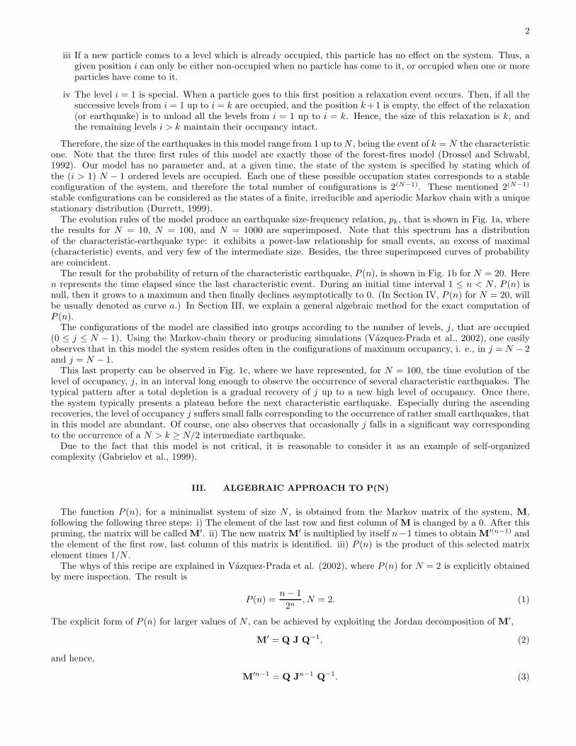
The evolution rules of the model produce an earthquake size-frequency relation, pk, that is shown in Fig. 1a, wherethe results for N = 10, N = 100, and N = 1000 are superimposed. Note that this spectrum has a distributionof the characteristic-earthquake type: it exhibits a power-law relationship for small events, an excess of maximal(characteristic) events, and very few of the intermediate size. Besides, the three superimposed curves of probabilityare coincident.

The result for the probability of return of the characteristic earthquake, P (n), is shown in Fig. 1b for N = 20. Heren represents the time elapsed since the last characteristic event. During an initial time interval 1 ≤ n < N , P (n) isnull, then it grows to a maximum and then finally declines asymptotically to 0. (In Section IV, P (n) for N = 20, willbe usually denoted as curve a.) In Section III, we explain a general algebraic method for the exact computation ofP (n).

The configurations of the model are classified into groups according to the number of levels, j, that are occupied(0 ≤ j ≤ N − 1). Using the Markov-chain theory or producing simulations (Vazquez-Prada et al., 2002), one easilyobserves that in this model the system resides often in the configurations of maximum occupancy, i. e., in j = N − 2and j = N − 1.

This last property can be observed in Fig. 1c, where we have represented, for N = 100, the time evolution of thelevel of occupancy, j, in an interval long enough to observe the occurrence of several characteristic earthquakes. Thetypical pattern after a total depletion is a gradual recovery of j up to a new high level of occupancy. Once there,the system typically presents a plateau before the next characteristic earthquake. Especially during the ascendingrecoveries, the level of occupancy j suffers small falls corresponding to the occurrence of rather small earthquakes, thatin this model are abundant. Of course, one also observes that occasionally j falls in a significant way correspondingto the occurrence of a N > k ≥ N/2 intermediate earthquake.

Due to the fact that this model is not critical, it is reasonable to consider it as an example of self-organizedcomplexity (Gabrielov et al., 1999).

III. ALGEBRAIC APPROACH TO P(N)

The function P (n), for a minimalist system of size N , is obtained from the Markov matrix of the system, M,following the following three steps: i) The element of the last row and first column of M is changed by a 0. After thispruning, the matrix will be called M′. ii) The new matrix M′ is multiplied by itself n−1 times to obtain M′(n−1) andthe element of the first row, last column of this matrix is identified. iii) P (n) is the product of this selected matrixelement times 1/N .

The whys of this recipe are explained in Vazquez-Prada et al. (2002), where P (n) for N = 2 is explicitly obtainedby mere inspection. The result is

P (n) =n − 1

2n, N = 2. (1)

The explicit form of P (n) for larger values of N , can be achieved by exploiting the Jordan decomposition of M′,

M′ = Q J Q−1, (2)

and hence,

M′n−1 = Q Jn−1 Q−1. (3)

3

1 10 100 1000

1E-5

1E-4

1E-3

0.01

0.1

1

a)

pk

k

0 100 200 300 400 500 600

0.000

0.002

0.004

0.006

0.008

0.010

b)

prob

abilit

y

n

12600 13300 14000 14700 15400

0

20

40

60

80

100

c)

occu

patio

n

t

FIG. 1: 1a) Probability of occurrence of earthquakes of size k. Note that the simulations corresponding to N equal to 10,100, and 1000 are superimposed. 1b) For N = 20, the probability of return of the characteristic earthquake as a function ofthe time elapsed since the last event, n. 1c) Time evolution of the state of occupation in a system of size N = 100. Note thatafter each characteristic event that completely depletes the system, there follows the corresponding recovery up to a high levelof occupancy, and then the system typically presents a plateau previous to the next characteristic earthquake.

4

The matrix J is formed by “Jordan blocks” in the diagonal positions, i.e., by square matrices whose elements arezero except for those on the principal diagonal, which are all equal, and those on the first superdiagonal, which areequal to unity. Thus, the task of obtaining an arbitrary power of J is simple because, as said, each Jordan block isthe sum of two conmuting matrices: one is a constant times the unity matrix, and the other is nilpotent. Therefore,in the computation of any arbitrary power of J, each block is independent and the corresponding Newton bynomialformula can be applied. As an example, we now present the calculation of the case N = 3. In this case,

3M′ =

1 1 1 00 2 0 11 0 1 10 0 0 2

, (4)

which is decomposed as

1 1 1 00 2 0 11 0 1 10 0 0 2

=

−1 1 1 20 0 2 −11 1 0 00 0 0 2

0 0 0 00 2 1 00 0 2 10 0 0 2

−1/2 1/4 1/2 −3/81/2 −1/4 1/2 3/8

0 1/2 0 1/40 0 0 1/2

. (5)

Therefore,

Jn−1 =

0 0 0 00 2n−1 (n − 1)2n−2 1/2(n− 1)(n − 2)2n−3

0 0 2n−1 (n − 1)2n−2

0 0 0 2n−1

(

1

3

)n−1

, (6)

and from eq. (3)

M′n−11,4 =

2n

32(n − 2)(n + 5)

(

1

3

)n−1

. (7)

Thus, finally,

P (n) =

(

2

3

)n(n − 2)(n + 5)

32, N = 3. (8)

One could optimistically guess that P (n), for an arbitrary N , can be deduced from the systematics observed in theprevious low-N cases. This is disproved by the following formula, which is the result of P (n) for N = 4.

P (n) =

(

1

4

)n [

−13

16+

7n

4−

n2

2+

n3

32+ 3n

[

−3

16+

7n

324+

n2

108+

n3

2599

]]

, N = 4. (9)

Although it is not apparent, this formula, as it should, vanishes for n = 3. As in eqs. (1) and (8), P (n) in eq. (9)is adequately normalized:

∞∑

n=N

P (n) = 1. (10)

IV. ERROR DIAGRAM FOR THE FORECASTING OF THE CHARACTERISTIC EARTHQUAKE

In the following paragraphs, we will stick to a model of size N = 20 to make the pertinent comparisons. This sizeis big enough for our purposes here, and small enough to obtain good statistics in the simulations.

For n = 20 the mean value of P (n) is

< n >=

∞∑

i=20

P (i)i = 121.05, (11)

5

the standard deviation is

σ =

[

∞∑

i=20

P (i)(i− < n >)2

]1/2

= 55.21, (12)

and the skew of the distribution is

γ =1

σ3

∞∑

i=20

P (i) · (i− < n >)3 = −0.10. (13)

Now we enter into the matter of forecasting. As in any optimization strategy, we will try to achieve simultaneouslythe most in a property called A and the least in a property called B, these two purposes being contradictory inthemselves. Here A is the (successful) forecast of the characteristic earthquakes produced in the system. Our desireis to forecast as many as possible, or ideally, all of them. B is the total amount of time that the earthquake alarm isswitched on during the forecasting process. As is obvious, our desire would be that this time were a minimum. Themaximization of A is equivalent to the minimization of an A′ that represents the fraction of unsuccessful forecasts.

Thus, in practice, our goal in this paper is to obtain simultaneously a minimum value for the two following functions,fe and fa. The first represents the fraction of unsuccessful forecasts, or fraction of failures; the second represents thefraction of alarm time. These two functions, in this first one-dimensional strategy of forecasting, are dependent onlyon the value of n, that is, the time elapsed since the last main event, and to which the alarm is connected. Using thefunction P (n) previously defined, they read as follows:

fe(n) =

n∑

n′=1

P (n′), (14)

fa(n) =

∑

∞

n′=n P (n′) (n′ − n)∑

∞

n′=0 P (n′) n′. (15)

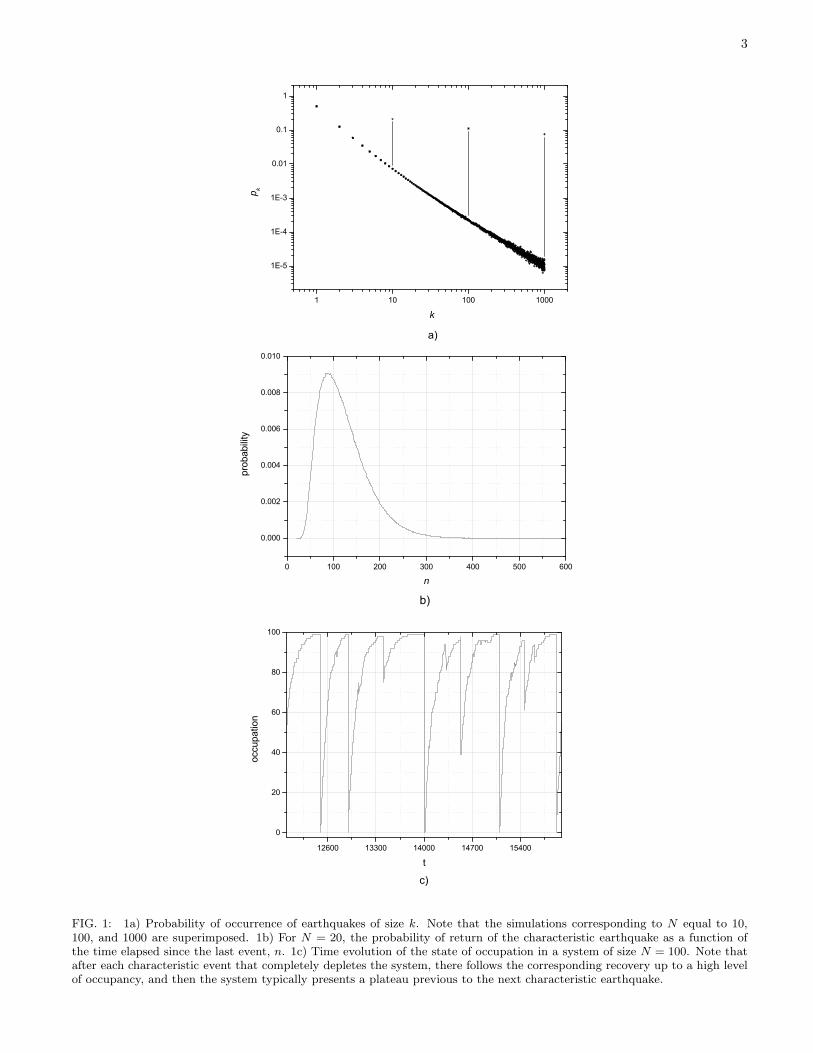
These two functions are plotted in Fig. 2a. By eliminating n between fe(n) and fa(n), we obtain Fig. 2b, which isthe standard form of representing the so-called error diagram. The diagonal straight line would represent the resultof a random forecasting strategy. The curved line is the result of this model.

Error diagrams were introduced in earthquake forecasting by Molchan who contributed with rigorous mathematicalanalysis to the optimization of the earthquake prediction strategies (Molchan, 1997). In his papers Molchan used τand n to represent the alarm fraction and the error fraction respectively; and put τ in the horizontal axis.

To fix ideas, it is convenient to define a so-called loss function, L, which expresses the trade-off between costs andbenefits in the forecasting (Keilis-Borok, 2002). Among all the possible loss functions, we will choose the simple linearfunction

L = fa + fe. (16)

L(n) is also drawn if Fig.2a. The position na = 66 provides the minimum value of L(n). L(na) = 0.578. Note thatna does not coincide either with the n that maximizes P (n), or with < n >.

V. IMPROVING THE FORECASTS

In Section IV we adopted the strategy of connecting the alarm at a fixed time, n, after the occurrence of acharacteristic event. The evaluation of this strategy leads to the conclusion that for n = na = 66, the loss functionhas a minimum value L(na) = 0.578. The question now is: Can we think up other strategies that render betterresults? To answer this question, we now return to our previous comments on Fig. 1.

If we define a medium-size earthquake as an event with a size between N/2 and N − 1, i.e. N > k ≥ N/2,by observing the graphs in Fig. 1, one is led to the conclusion that in this model the occurrence of a medium-sizeearthquake is not frequent but when it actually takes place, the time of return of the characteristic quake in thatcycle is increased.

This qualitative perception can be substantiated by numerically obtaining the probability of having cycles whereno medium-size earthquake occurs, i.e., k < N/2. This information is completed by the distribution of cycles where

6

0 100 200 300 400 500 600 700 800 900

0.0

0.2

0.4

0.6

0.8

1.0

na=66

L(n)

a)

fa(n)

fe(n)

fa

(n),

fe(n

), L(

n)

n0.0 0.2 0.4 0.6 0.8 1.0

0.0

0.2

0.4

0.6

0.8

1.0

b)

na=66

fa(n

)

fe(n)

FIG. 2: For N = 20, a) Fraction of failures to predict, fe, fraction of alarm time, fa, and loss function L = fa +fe as a functionof n. b) Error diagram for characteristic event forecasts based on n. The diagonal line would correspond to a random strategy.

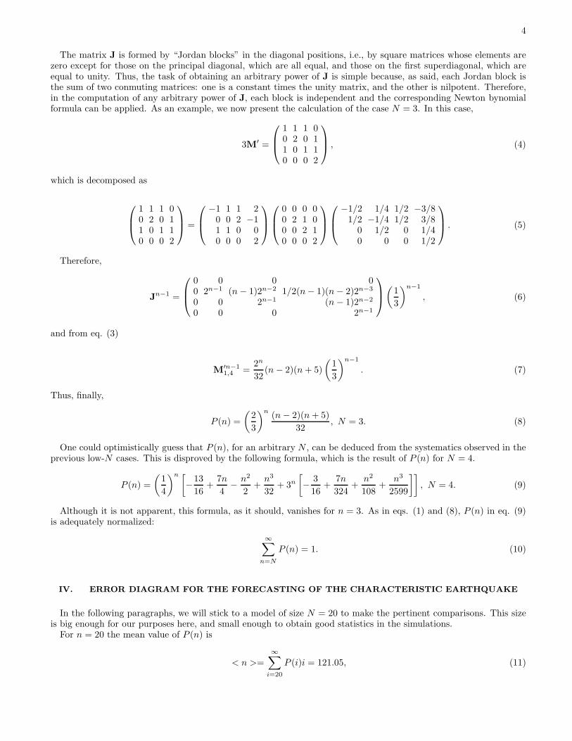
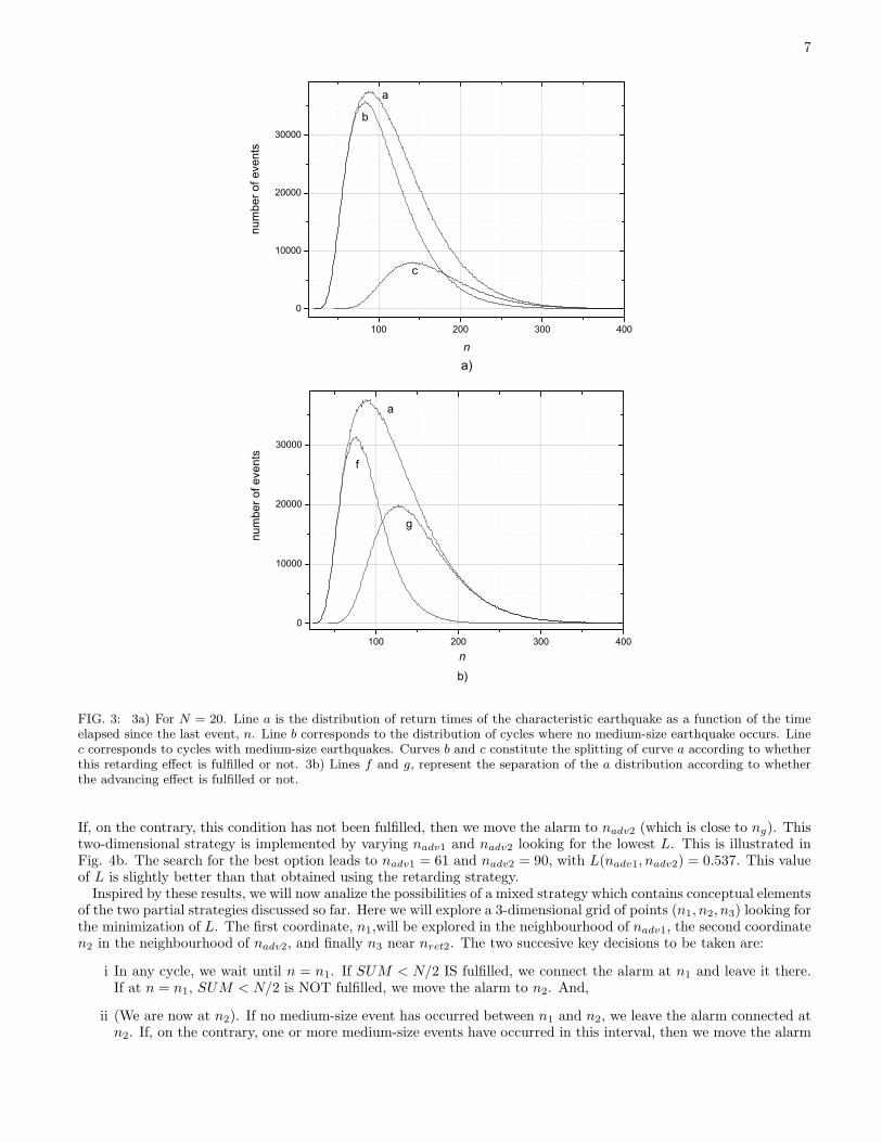
the condition N > k ≥ N/2 does occur. These two distributions are shown in Fig. 3a as lines b and c respectively.Here, line a represents the total distribution of the times of return of the characteristic earthquake in this model (thesame as plotted in Fig. 1b). Note that, as it should, the distribution a covers both distributions b and c. The meantime < n > for the three distributions is < n >a= 121.05, < n >b= 107.57 and < n >c= 166.84. The fraction ofcycles under b is 0.77 and the fraction under c is 0.23. A splitting of this type, in which the a distribution separatesinto b and c, will be denoted henceforth as a = b ⊕ c.

To check if a = b ⊕ c is potentially useful for our purposes, we will now analyze independently these two sets ofcycles, b and c, with the method used in Section IV for curve a. The result is the following: the best working n fordealing with the cycles under distribution b is nb = 60. And with respect to the cycles belonging to the distributionunder c, the best n is nc = 124.

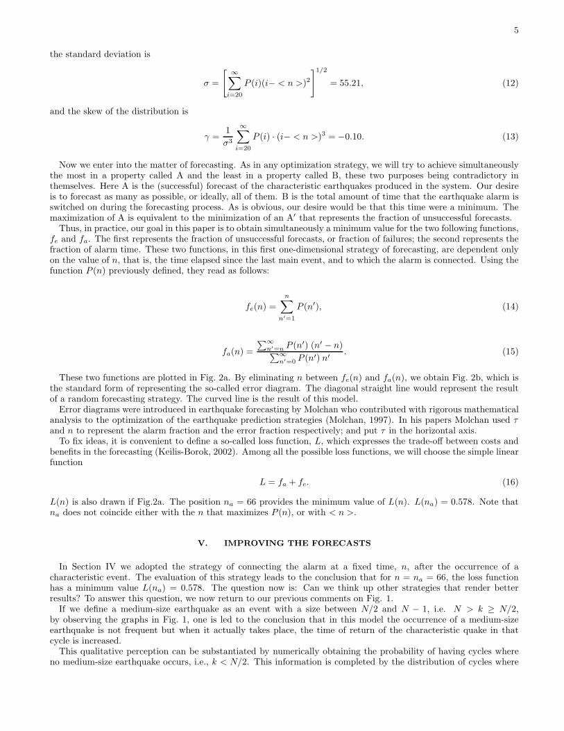
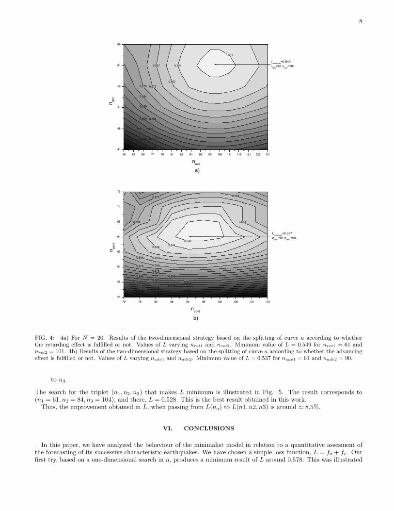
Therefore, we will now study again the whole set of cycles, i.e. those under a, by means of a retarding strategy,which is based on the splitting a = b ⊕ c. We will adopt the following steps: in any cycle, we will wait until an n,named nret1 (which is near to nb), before taking any decision. If no medium earthquake has occurred so far, then thealarm is connected at nret1. If, on the contrary, a medium quake has occurred before nret1, then we move the alarmto nret2 (which is close to nc). This notation nret1 and nret2 comes from the retarding strategy that we are exploringnow. This two-dimensional strategy is implemented by varying nret1 and nret2 looking for the best value of L. Thisis illustrated in Fig. 4a. The best option is nret1 = 61 and nret2 = 101, with L(nret1, nret2) = 0.549.

Now we look for a similar property that can classify the cycles from another point of view. This new propertyconsists in identifying the cycles where the sum of the sizes of all the earthquakes before the characteristic one is lessthan N/2. This condition will be represented by SUM < N/2. The reason for this choice is that if SUM < N/2,the system, statistically speaking, tends to reach more rapidly the configurations of maximum occupancy, j = N − 2and j = N − 1, and the time of return of the characteristic quake in that cycle tends to be smaller (see Fig. 1c). InFig. 3b, line a represents, as in Fig. 3a, the distribution of return intervals of the characteristic earthquake for all thecycles of the model. And lines f and g represent, respectively, the separation of line a according to the fulfilment, ornot, of the SUM < N/2 condition, a = f ⊕ g. The mean value of the f and g distributions is < n >f= 88.78 and< n >g= 151.69 respectively. The fraction of events under the f and g lines is 36.96 and 63.04 respectively.

This second splitting of the whole set of cycles in the model, a = f ⊕ g, can be used as an advancing strategy inparallel to what we did with the retarding strategy. Thus the independent analysis of curve f leads to nf = 60, andthe similar analysis of curve g leads to ng = 90.

We will now study again the whole set of cycles (under a) by means of the advancing strategy, which is based onthe splitting a = f ⊕ g. Therefore, we proceed as follows: In any cycle, we wait until nadv1 (which is close to nf )before taking any decision. If the condition SUM < N/2 has been fulfilled, then the alarm is connected at n = nadv1.

7

100 200 300 400

0

10000

20000

30000

a)

c

b

a

num

ber o

f eve

nts

n

100 200 300 400

0

10000

20000

30000

b)

g

f

a

num

ber o

f eve

nts

n

FIG. 3: 3a) For N = 20. Line a is the distribution of return times of the characteristic earthquake as a function of the timeelapsed since the last event, n. Line b corresponds to the distribution of cycles where no medium-size earthquake occurs. Linec corresponds to cycles with medium-size earthquakes. Curves b and c constitute the splitting of curve a according to whetherthis retarding effect is fulfilled or not. 3b) Lines f and g, represent the separation of the a distribution according to whetherthe advancing effect is fulfilled or not.

If, on the contrary, this condition has not been fulfilled, then we move the alarm to nadv2 (which is close to ng). Thistwo-dimensional strategy is implemented by varying nadv1 and nadv2 looking for the lowest L. This is illustrated inFig. 4b. The search for the best option leads to nadv1 = 61 and nadv2 = 90, with L(nadv1, nadv2) = 0.537. This valueof L is slightly better than that obtained using the retarding strategy.

Inspired by these results, we will now analize the possibilities of a mixed strategy which contains conceptual elementsof the two partial strategies discussed so far. Here we will explore a 3-dimensional grid of points (n1, n2, n3) looking forthe minimization of L. The first coordinate, n1,will be explored in the neighbourhood of nadv1, the second coordinaten2 in the neighbourhood of nadv2, and finally n3 near nret2. The two succesive key decisions to be taken are:

i In any cycle, we wait until n = n1. If SUM < N/2 IS fulfilled, we connect the alarm at n1 and leave it there.If at n = n1, SUM < N/2 is NOT fulfilled, we move the alarm to n2. And,

ii (We are now at n2). If no medium-size event has occurred between n1 and n2, we leave the alarm connected atn2. If, on the contrary, one or more medium-size events have occurred in this interval, then we move the alarm

8

0.633 0.628

0.622 0.617

0.611 0.606

0.600 0.595

0.589

0.584

0.578 0.573

0.567

0.562

0.556

0.551

56 61 66 71 76 81 86 91 96 101 106 111 116 121 126 131

41

46

51

56

61

66

a)

Lminimum=0.549nret1=61,nret2=101

n ret1

nret2

0.6400.6360.6310.626 0.621

0.616 0.6120.607 0.602

0.5970.592 0.588

0.5830.578

0.573 0.568

0.564 0.559

0.554

0.564

0.568

0.573

0.549 0.5440.540

70 75 80 85 90 95 100 105 110 115

41

46

51

56

61

66

71

76

b)

Lminimum=0.537nadv1=61,nadv2=90

n adv

1

nadv2

FIG. 4: 4a) For N = 20. Results of the two-dimensional strategy based on the splitting of curve a according to whetherthe retarding effect is fulfilled or not. Values of L varying nret1 and nret2. Minimum value of L = 0.549 for nret1 = 61 andnret2 = 101. 4b) Results of the two-dimensional strategy based on the splitting of curve a according to whether the advancingeffect is fulfilled or not. Values of L varying nadv1 and nadv2. Minimum value of L = 0.537 for nadv1 = 61 and nadv2 = 90.

to n3.

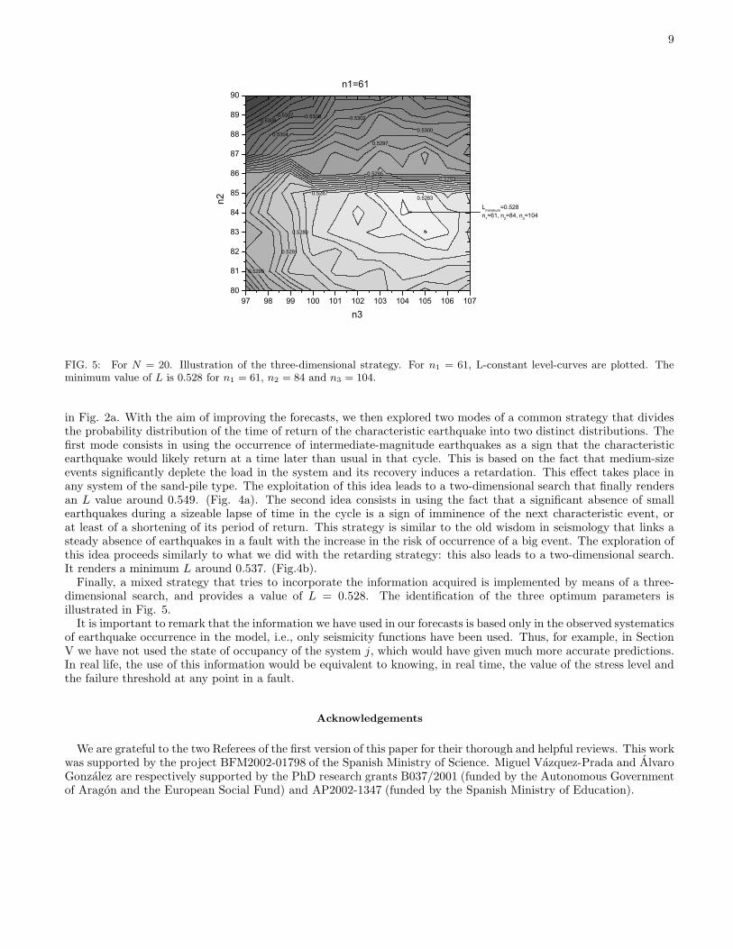
The search for the triplet (n1, n2, n3) that makes L minimum is illustrated in Fig. 5. The result corresponds to(n1 = 61, n2 = 84, n3 = 104), and there, L = 0.528. This is the best result obtained in this work.

Thus, the improvement obtained in L, when passing from L(na) to L(n1, n2, n3) is around ≃ 8.5%.

VI. CONCLUSIONS

In this paper, we have analyzed the behaviour of the minimalist model in relation to a quantitative assesment ofthe forecasting of its successive characteristic earthquakes. We have chosen a simple loss function, L = fa + fe. Ourfirst try, based on a one-dimensional search in n, produces a minimum result of L around 0.578. This was illustrated

9

0.5295

0.5293

0.5291

0.5295

0.5289

0.5297

0.5287

0.5300

0.5302

0.5304

0.53060.53070.5308

0.5283

97 98 99 100 101 102 103 104 105 106 10780

81

82

83

84

85

86

87

88

89

90

Lminimum=0.528n1=61, n2=84, n3=104

n1=61

n3

n2

FIG. 5: For N = 20. Illustration of the three-dimensional strategy. For n1 = 61, L-constant level-curves are plotted. Theminimum value of L is 0.528 for n1 = 61, n2 = 84 and n3 = 104.

in Fig. 2a. With the aim of improving the forecasts, we then explored two modes of a common strategy that dividesthe probability distribution of the time of return of the characteristic earthquake into two distinct distributions. Thefirst mode consists in using the occurrence of intermediate-magnitude earthquakes as a sign that the characteristicearthquake would likely return at a time later than usual in that cycle. This is based on the fact that medium-sizeevents significantly deplete the load in the system and its recovery induces a retardation. This effect takes place inany system of the sand-pile type. The exploitation of this idea leads to a two-dimensional search that finally rendersan L value around 0.549. (Fig. 4a). The second idea consists in using the fact that a significant absence of smallearthquakes during a sizeable lapse of time in the cycle is a sign of imminence of the next characteristic event, orat least of a shortening of its period of return. This strategy is similar to the old wisdom in seismology that links asteady absence of earthquakes in a fault with the increase in the risk of occurrence of a big event. The exploration ofthis idea proceeds similarly to what we did with the retarding strategy: this also leads to a two-dimensional search.It renders a minimum L around 0.537. (Fig.4b).

Finally, a mixed strategy that tries to incorporate the information acquired is implemented by means of a three-dimensional search, and provides a value of L = 0.528. The identification of the three optimum parameters isillustrated in Fig. 5.

It is important to remark that the information we have used in our forecasts is based only in the observed systematicsof earthquake occurrence in the model, i.e., only seismicity functions have been used. Thus, for example, in SectionV we have not used the state of occupancy of the system j, which would have given much more accurate predictions.In real life, the use of this information would be equivalent to knowing, in real time, the value of the stress level andthe failure threshold at any point in a fault.

Acknowledgements

We are grateful to the two Referees of the first version of this paper for their thorough and helpful reviews. This workwas supported by the project BFM2002-01798 of the Spanish Ministry of Science. Miguel Vazquez-Prada and AlvaroGonzalez are respectively supported by the PhD research grants B037/2001 (funded by the Autonomous Governmentof Aragon and the European Social Fund) and AP2002-1347 (funded by the Spanish Ministry of Education).

10

References

Ben-Zion, Y., Eneva, M., and Liu, Y.: Large Earthquake Cycles and Intermittent Criticality On Heterogeneous FaultsDue To Evolving Stress And Seismicity, J. Geophys. Res., 108 (B6), 2307, doi: 10.1029/2002JB002121, 2003.Dahmen, K., Ertas, D., and Ben-Zion, Y.: Gutenberg-Richter and characteristic behaviour in simple mean-fieldmodels of heterogeneous faults, Phys. Rev., E58, 1444-1501, 1998.Drossel, B., and Schwabl, F.: Self-organized critical forest-fire model, Phys. Rev. Lett., 69, 1629-1632, 1992.Durrett, R.: Essentials of Stochastic Processes, Chapter 1, Springer, 1999.Gabrielov, A., Newman, W. I., and Turcotte, D. L.: Exactly soluble hierarchical clustering model: inverse cascades,self-similarity and scaling, Phys. Rev., E60, 5293-5300, 1999.Gabrielov, A., Zaliapin, I., Newman, W., and Keilis-Borok, V. I.: Colliding cascades model for earthquake prediction,Geophys. J. Int., 143, 427-437, 2000.Keilis-Borok, V.: Earthquake Prediction: State-of-the-Art and Emerging Possibilities, Annu. Rev. Earth Planet.Sci., 30, 1-33, 2002.Keilis-Borok, V. I., and Soloviev, A. A. (Eds.): Nonlinear Dynamics of the Lithosphere and Earthquake Prediction,Springer, 2002.Lomnitz, C.: Fundamentals of Earthquake Prediction, J. Wiley & Sons, 1994.Molchan, G. M.: Earthquake Prediction as a Decision-making Problem, Pure. Appl. Geophys., 149, 233-247, 1997.Newman W. I., and Turcotte, D. L.: A simple model for the earthquake cycle combining self-organized complexitywith critical point behavior, Nonlin. Proces. Geophys., 9, 453-461, 2002.Sornette, D.: Critical Phenomena in Natural Sciences, Springer Verlag, Berlin, Germany, 2000.Schwartz, D.P. and Coppersmith, K. J.: Fault behaviour and characteristic earthquakes: Examples from the Wasatchand San Andreas Fault Zones, J. Geophys. Res., 89, 5681-5698, 1984.Turcotte, D. L.: Fractals and Chaos in Geophysics, 2nd Edit., Cambridge Univ. Press, 2000.Vazquez-Prada, M., Gonzalez, A., Gomez, J. B., and Pacheco, A. F.: A Minimalist model of characteristic earthquakes,Nonlin. Proces. Geophys., 9, 513-519, 2002.Wesnousky, S. G.: The Gutenberg-Richter or Characteristic-Earthquake Distribution, Wich It Is?, Bull. Seism. Soc.Am., 84, 1940-1959, 1994.