Multisectoral Approach to the Prevention and Control of Vector ...

Singular & Characteristic Structures
of Similar Multisectoral Systems
Adamou, N.1 & M. Ciaschini2
12th International Conference of Input-Output TechniquesNew York University, May 18 - 22, 1998
Section 5.3 Application of Mathematical Techniques Tuesday, May 19, Room #408
Abstract: Singular as well as eigen decomposition are used examining similar linearmultisectoral systems. Linear transformations examining the relations between the singular valuesof the Leontief and its similar inverse, as well as singular and characteristic values specify theintrinsic structures based on eigenvector relations. Four specific structures are examined. Thestructure that associates the common eigenvalues of the Leontief and its similar inverses to theirdifferent eigenvectors. Second examined structure is the one that relates eigen to singular values.Finally, the two alternative ways transform the singular values of the Leontief inverse into thesingular values of its similar inverse are examined. A pragmatic example demonstrates thetheoretical exploration.
1 Introduction
Similar multisectoral linear systems are analyzed combining singular and eigen value decomposition.Thus, intrinsic structural characteristics of the entailed linear transformations are formed by the pertinenteigenvectors.
Similarity transformation between two matrices lays its foundation on the change of a basis of a matrix.
Direct purchases A ↑[ ] as well as direct sales r B [ ] are defined on the space of interindustry transactions in
their proportion to sectoral gross output.3 The diagonal matrix of gross output and its inverse serve astransition matrices of the similarity transformation.4 The same similarity transformation relates matrices
I − A ↑[ ] to I −
r B [ ] as well as their inverses Z and G . Similar matrices are equivalent to each other,
having common determinants and eigenvalues. The eigenvalues may be real or complex, based upon therelation between the trace and determinant. The corresponding eigenvectors are different for matrices Zand G . All matrices of the purchase requirement perspective5 have the same eigenvectors, while theireigenvalues are linearly related. The same holds true for their similar matrices of the sale allocationstandpoint.6
Singular value decomposition was proposed as an alternative to the traditional multisectoral multiplier,and their associated orthogonal matrices offer a way to analyze the intersectoral structure. Matrices Zand G , although they share common eigenvalues, have different real and distinct singular values.Eigenvalues were suggested as an impact measurement as well. Yet, although both singular values andeigenvalues were assumed to measure impact, a comparative examination of singular and eigen valuesprovided diverge results. This leads to an exploration of the relations between singular and eigen valuesand their structural implications in impact analysis. Singular and eigen values are independent of anypermutation of the productive interdependent sectors, while the associated vectors of the appropriatedecomposition reflect the applied sectoral permutation. This result leads one to examine the vectorspaces in their association to singular and eigenvalues of the Leontief and its similar inverses. Such anexamination of the spaces and structures formed by the linear transformations based on singular and eigen
1 Aristotelian University of Thessaloniki, School of Law & Economics, Greece.2 University of Macerata, Faculty of Law, Italy.3 A ↑[ ] = X[ ] diag x( )[ ]−1
and r B [ ] = diag x( )[ ]−1 X[ ].
4 A ↑[ ] = diag x( )[ ]
r B [ ] diag x( )[ ]−1
.
5 A ↑[ ] , I − A ↑[ ] and Z = I − A↑[ ] −1.
6 r B [ ] ,
I −
r B [ ] , and
G = I −
r B [ ] .

Singular & Characteristic Structures of Similar Multisectoral Systems2
value decomposition of similar matrices illuminates the intrinsic structure of a multisectoral linearsystem. This paper examines the linear transformations that relate singular and eigen values, as well asthe two different sets of singular values of similar matrices. Figure 1-A shows the objective of the paper.
Figure 1-A
Common Eigenvalues of Leontief & its Similar Inverse
Singular Values of Leontief Inverse
Singular Values of Similar LeontiefInverse
Λ
SGSZ
Relationships among Eigen & Singular Values
The involved eigenvectors determine the structure of the above mentioned linear transformations,presented in Figure 1-B.
Figure 1-B
Structures Relating Eigen & Singular Values
Λ
SZ SG
Eigevectors of the Leontief Inverse & its similar associated to the eigen- values in correspondence with the diag. gross output
m
zev zeu zsev zseu
yv yu
kv ku
Eigenvectors of the Leontief Inverse &its similar related to Orthogonal Matrices of the SVD
y relationship between Singular Values
through z structures
k relationship between Singular Valuesthrough the Orthogonal Matrices of the SVDand diag. gross output
The structural information used are presented in Figure 2. The Leontief and its similar inverse have thesame eigenvalues and different eigenvectors, while there are decomposed in different singular valueterms.

Adamou, & Ciaschini, 12th International Conference of Input-Output Techniques 3
Figure 2
l1
ln
O
SL1
SLn
SGn
SGn
O
O
0
0 0
0
0
0ez1 ezn eg1 egn
vz1 vzn uz1 uzn vg1 vgn u g1 ugn
M
M
M
M
M
M
M
M
M
M
M
M
M
M
M
M
M
M
M
M
M
M
M
M
L
L
L
L
L
L
Eigenvectors
of Leontief Inverse
Eigenvectors of
similar Leontief Inverse
Eigenvalues
Singular Values
Left Orthogonal
RightOrthogonal
Left Orthogonal
RightOrthogonal
Singular Values
Leontief Inverse
Similar Leontief Inverse
2 Methodology
The Leontief inverse matrix Z and its similar G have the same eigenvalues Λ , while their respectiveassociated eigenvectors EZ and EG are different from each other providing the following decomposition:
(1) Z = EZΛEZ−1 G = EG Λ EG
−1
The real symmetric matrices normal7 ZTZ[ ] and GTG[ ] guarantee real and distinct eigenvalues, while
matrices Z and G may have complex conjugate eigenvalues. The square root of eigenvalues of the
symmetric matrices are the singular values SZ and SG . The matrix decomposition of ZTZ[ ] and GTG[ ]in terms of their own eigenvalues SZ
2 & SG2 and their corresponding matrices of orthonormal eigenvectors
U Z & UG , is known as spectral decomposition or principal axis theorem
(2) ZTZ[ ] = UZTSZ
2 U Z[ ] GTG[ ] =
UG
T SG2 UG[ ] .
Given matrices Z & G , eigenvectors, U L & UG , and the reciprocal of the square roots of eigenvalues,
SL−1 and SG
−1, one may define matrices V L and VG as V Z = ZU Z S Z−1 and VG = GUG SG
−1. Then, the
singular value decomposition of matrices Z & G are:
(3) Z = VZSZUZT G = VG SG UG
T .
Matrices V Z , VG , U Z and UG are orthogonal.8
7 Normal is a matrix that possesses a complete set of orthonormal eigenvectors, Strang (1988), p. 311.8 Orthogonal matrix means that the product of the matrix to its transpose is the identity matrix, and its transposed equals its
inverse. The first statement says, in other words, that any column multiplied by its appropriate row yields one, and thevalue of a column element is the reciprocal of the value of the appropriate row element. This indicates that columns of an

Singular & Characteristic Structures of Similar Multisectoral Systems4
The unitary matrices of eigenvectors U ZT and VG
T were called reference structure for final use and value
added respectively and V ZT and UG
T the reference structures of production and allocation for grossoutput. It was argued that the columns of the reference structure need to be taken into considerationinstead of the unitary multipliers.9
In a similar manner, one may identify the decomposition of the eigenvalues Λ of similar matrices.
Simplifying by µ[ ] = EZ−1 diag x( )EG[ ] , we have
(4) Λ = µ[ ]Λ µ−1[ ] .
Structure µ[ ] relates the inverse of eigenvectors of the Leontief inverse to the eigenvectors of its similarinverse through the diagonal of gross output. This decomposition of eigenvalues provides the structure ofthe interrelation of eigenvectors of similar matrices though the transition matrix of gross output.
The structures relating eigenvectors to the right and left orthogonal matrices of the singular value
decomposition are ζev[ ] = EZ−1V Z[ ] , ζeu[ ] = U Z
T EZ[ ] , ζevs[ ] = EG
−1V G[ ] , and ζeus[ ] = UG
T EG[ ] . These
structures transform the common eigenvalues into different singular values as:
(5) Λ = ζev[ ] SZ ζeu[ ] = ζevs[ ] SG ζeu
s[ ] .
Figure 3
E
V
-1
Z
Z
zev
z
SZ
eu
U
EZ
Z
T
S SL =Z
L z z=ev eu
s s
E
EV
U
G
-1 T
G
G
G
G
SG
This leads towards the transformation of the singular values of the similar matrix as:
SZ = V ZT EZ EG
−1( )VG[ ] SG UGT EG EZ
−1( )U Z[ ] ⇔ SZ = VZT η1( ) VG[ ]SG UG
T η1−1( )U Z[ ]
(6) SZ = ψ v[ ] SG ψu[ ]
where η[ ] = EZEG−1[ ] , ψv[ ] = ζev
−1ζevs[ ] , and ψu[ ] = ζeu
s ζeu−1[ ] . Structure η[ ] gives the direct relation of
eigenvectors of similar matrices, while structure µ[ ] diagonalizes this relation by incorporating thediagonal gross output.
orthogonal matrix are orthonormal. Orthonormal eigenvectors are orthogonal scaled to a unit length. Strang (1988),pp.296-297.
9 Ciaschini, M. (1993) op. cit., p. 146.

Adamou, & Ciaschini, 12th International Conference of Input-Output Techniques 5
Figure 4
SZ
SG
VZ
T
EZ
EG
−1
VG
h
UG
T
EG
EZ
−1
UZ
−1h
= y yV U
SG
Combining similarity to the singular value decomposition of Z and G we have
SZ = V ZT diag x( )[ ]VG[ ] SG UG
T diag x( )[ ]−1 U Z[ ] , or:
(7) SZ = κ v[ ] SG κ u[ ]
where κv[ ] = V ZT diag x( )[ ]VG[ ] and κu[ ] = UG
T diag x( )[ ]−1 UZ[ ] .
Figure 5
SZ
SG
VZ
T VG
UG
TU
Z
= k kV U
SG
diag (x) diag (x)-1
Singular & Characteristic Structures of Similar Multisectoral Systems6
Structure κv[ ] relates the left eigenspace of the singular value decomposition of similar matrices through
the diagonal of gross output. In the same way, structure κu[ ] relates the right eigenspace of the singularvalue decomposition of similar matrices through the diagonal of gross output.
Structures κv[ ] & ψv[ ] and κu[ ] & ψu[ ] , respectively, are equivalent.
3 Concluding Implications

Adamou, & Ciaschini, 12th International Conference of Input-Output Techniques 7
Singular Values of the Leontief Inverse
R2 = 0.9602
0.0
0.5
1.0
1.5
2.0
2.5
3.0
3.5
1955 1960 1965 1970 1975 1980 1985
Singular Values of the Similar Leontief Inverse
R2 = 0.979
0
2
4
6
8
10
12
14
16
1955 1960 1965 1970 1975 1980 1985
Eigenvalues of the Leontief Inverse
R2 = 0.9797
0.0
0.5
1.0
1.5
2.0
2.5
1955 1960 1965 1970 1975 1980 1985

Singular & Characteristic Structures of Similar Multisectoral Systems8
Singular Values of the Leontief Inverse1955 1960 1965 1970 1975 1980 1985
1 3.04 3.19 3.00 2.75 2.96 3.22 2.912 1.16 1.16 1.12 1.14 1.21 1.17 1.163 1.13 1.10 1.07 1.08 1.15 1.12 1.104 1.10 1.06 1.06 1.08 1.09 1.08 1.085 1.03 1.05 1.05 1.03 1.05 1.04 1.076 1.01 1.04 1.04 1.02 1.04 1.03 1.027 1.00 1.02 1.01 1.02 1.01 1.02 1.028 1.00 1.00 1.00 1.00 1.00 0.99 1.009 0.99 1.00 1.00 0.99 0.99 0.99 0.9910 0.96 0.99 0.99 0.98 0.97 0.98 0.9811 0.95 0.96 0.97 0.96 0.90 0.96 0.9812 0.90 0.92 0.95 0.95 0.86 0.90 0.9313 0.67 0.73 0.73 0.80 0.77 0.75 0.76
Singular Values of the Similar Leontief Inverse1955 1960 1965 1970 1975 1980 1985
1 3.94 5.34 5.76 6.73 12.20 13.70 11.902 1.32 1.31 1.33 1.38 1.45 1.48 1.463 1.14 1.17 1.15 1.16 1.14 1.17 1.184 1.10 1.08 1.06 1.09 1.10 1.13 1.085 1.05 1.03 1.04 1.06 1.06 1.08 1.056 1.02 1.02 1.03 1.02 1.03 1.02 1.037 1.01 1.01 1.01 1.01 1.01 1.00 1.018 1.00 0.99 0.98 1.00 1.00 0.98 1.009 0.95 0.98 0.98 0.98 0.97 0.98 0.9810 0.94 0.94 0.97 0.97 0.94 0.96 0.9711 0.93 0.93 0.95 0.94 0.93 0.91 0.8912 0.79 0.83 0.82 0.79 0.81 0.78 0.8113 0.54 0.45 0.37 0.32 0.17 0.16 0.18
Eigenvalues of the Leontief Inverse1955 1960 1965 1970 1975 1980 1985
1 2.16 2.42 2.27 2.24 2.36 2.48 2.292 1.10 1.15 1.10 1.14 1.14 1.15 1.163 1.07 0.06 1.07 0.04 1.05 1.09 1.09 1.04 0.08 1.094 1.07 -0.06 1.07 -0.04 1.05 0.03 1.08 1.05 0.10 1.04 -0.08 1.085 1.04 1.06 1.05 -0.03 1.03 0.03 1.05 -0.10 1.03 0.01 1.03 0.056 1.02 1.03 1.03 1.03 -0.03 1.01 1.03 -0.01 1.03 -0.057 1.00 1.00 0.00 1.00 0.01 1.00 1.00 1.00 0.01 1.018 1.00 1.00 0.00 1.00 -0.01 1.00 0.99 0.02 1.00 -0.01 1.009 1.00 0.02 1.00 0.03 1.00 0.99 0.99 -0.02 1.00 0.02 0.98 0.02
10 1.00 -0.02 1.00 -0.03 0.99 0.04 0.98 0.98 0.09 1.00 -0.02 0.98 -0.0211 0.96 0.99 0.99 -0.04 0.97 0.98 -0.09 0.99 0.98 0.0112 0.95 0.03 0.94 0.01 0.98 0.97 0.05 0.95 0.02 0.97 0.06 0.98 -0.0113 0.95 -0.03 0.94 -0.01 0.96 0.97 -0.05 0.95 -0.02 0.97 -0.06 0.96
Adamou, & Ciaschini, 12th International Conference of Input-Output Techniques 9
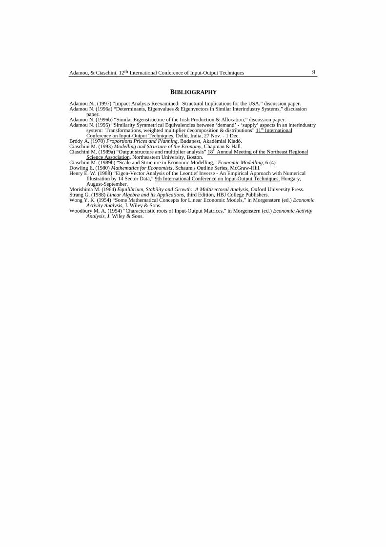
BIBLIOGRAPHY
Adamou N., (1997) “Impact Analysis Reexamined: Structural Implications for the USA,” discussion paper.Adamou N. (1996a) “Determinants, Eigenvalues & Eigenvectors in Similar Interindustry Systems,” discussion
paper.Adamou N. (1996b) “Similar Eigenstructure of the Irish Production & Allocation,” discussion paper.Adamou N. (1995) “Similarity Symmetrical Equivalencies between ‘demand’ - ‘supply’ aspects in an interindustry
system: Transformations, weighted multiplier decomposition & distributions” 11th InternationalConference on Input-Output Techniques, Delhi, India, 27 Nov. - 1 Dec.
Bródy A. (1970) Proportions Prices and Planning, Budapest, Akadémiai Kiadó.Ciaschini M. (1993) Modelling and Structure of the Economy, Chapman & Hall.Ciaschini M. (1989a) “Output structure and multiplier analysis” 18th Annual Meeting of the Northeast Regional
Science Association, Northeastern University, Boston.Ciaschini M. (1989b) “Scale and Structure in Economic Modelling,” Economic Modelling, 6 (4).Dowling E. (1980) Mathematics for Economists, Schaum's Outline Series, McGraw-Hill.Henry E. W. (1988) “Eigen-Vector Analysis of the Leontief Inverse - An Empirical Approach with Numerical
Illustration by 14 Sector Data,” 9th International Conference on Input-Output Techniques, Hungary,August-September.
Morishima M. (1964) Equilibrium, Stability and Growth: A Multisectoral Analysis, Oxford University Press.Strang G. (1988) Linear Algebra and its Applications, third Edition, HBJ College Publishers.Wong Y. K. (1954) “Some Mathematical Concepts for Linear Economic Models,” in Morgenstern (ed.) Economic
Activity Analysis, J. Wiley & Sons.Woodbury M. A. (1954) “Characteristic roots of Input-Output Matrices,” in Morgenstern (ed.) Economic Activity
Analysis, J. Wiley & Sons.

Singular & Characteristic Structures of Similar Multisectoral Systems10
Descriptive Visual Appendix
Italian Three Sector Graphical Presentation of Matrix Structures
Leontief Inverse
Z =1.212 0.073 0.019
0.293 1.622 0.267
0.112 0.208 1.221
Similar Leontief Inverse
G =1.212 0.961 0.178
0.022 1.622 0.191
0.012 0.290 1.221
The roots of the characteristic polynomial of the Leontief inversef t( ) =− t3 + 4.056 t 2 − 5.352t + 2.309
are its eigenvalues.

Adamou, & Ciaschini, 12th International Conference of Input-Output Techniques 11
Eigenvalues of the Leontief Inverse
Λ =1.77384 0 0
0 1.17253 0
0 0 1.1106
Eigenvectors of the Leontief Inverse
EZ =0.133 0.871 0.255
0.917 −0.405 −0.558
0.374 −0.275 0.788
Eigenvectors of the Leontief Similar Inverse
EG =−0.854 −0.998 0.937
−0.450 0.035 −0.157
−0.256 0.033 0.309
Singular Values of the Leontief Inverse
SZ =1.802 0 0
0 1.158 0
0 0 1.106

Singular & Characteristic Structures of Similar Multisectoral Systems12
Singular Values of the Leontief Similar Inverse
SG =2.106 0 0
0 1.157 0
0 0 0.947
Left eigenvector of the Leontief's inverse Singular Value Decomposition
V Z =−0.276 0.910 0.307
−0.878 −0.110 −0.464
−0.389 −0.398 0.830
Right eigenvector of the Leontief's inverse Singular Value Decomposition
U ZT =
−0.353 −0.846 −0.396
0.886 −0.168 −0.430
0.298 −0.504 0.810
Left eigenvector of the Similar Leontief's inverse Singular Value Decomposition
VG =−0.644 −0.364 0.671
−0.707 −0.048 −0.705
−0.290 0.929 0.226

Adamou, & Ciaschini, 12th International Conference of Input-Output Techniques 13
Right eigenvector of the Similar Leontief's inverse Singular Value Decomposition
UGT =
−0.380 −0.879 −0.287
−0.373 −0.138 0.917
0.845 −0.456 0.275
Diagonal Matrix of Gross Output
diag x( ) =0.727 0 0
0 9.487 0
0 0 6.810
Eigenvectors of the Leontief inverse multiplied to the inverse Eigenvectors of the Leontief similarinverse
η = EZEG−1[ ]
η =−0.789 −0.490 2.974
0.273 −0.816 −3.054
0.242 −1.802 0.900
µ = EZ−1diag x( )EG[ ]
µ =−4.663 0 0
0 −0.833 0
0 0 2.667

Singular & Characteristic Structures of Similar Multisectoral Systems14
ζev = EZ−1V Z[ ]
ζev =−1.048 0.216 0.123
−0.143 1.079 0.037
−0.045 −0.230 1.007
ζeu = U ZT EZ[ ]
ζeu =−0.972 0.144 0.069
−0.197 0.959 −0.019
−0.119 0.240 0.997
ζevs = EG
−1VG[ ]
ζevs =
1.441 −0.463 1.010
−0.314 2.926 −0.055
0.291 2.304 1.577
ζeus = UG
T EG[ ]
ζeus =
0.795 0.338 −0.307
0.146 0.399 −0.045
−0.588 −0.851 0.950
Adamou, & Ciaschini, 12th International Conference of Input-Output Techniques 15
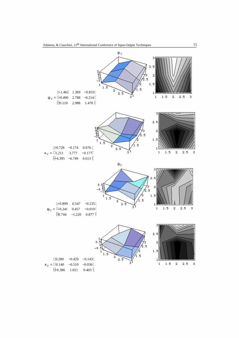
ψ V
ψ V =−1.462 1.369 −0.833
−0.490 2.788 −0.214
0.110 2.988 1.478
κ V =−0.728 −0.174 0.676
1.211 3.777 −0.177
−4.395 −6.749 6.613
ψU
ψU =−0.899 0.547 −0.235
−0.241 0.457 −0.019
0.744 −1.220 0.877
κU =0.280 −0.429 −0.143
0.140 −0.510 −0.036
−0.386 1.021 0.403

Singular & Characteristic Structures of Similar Multisectoral Systems16
Analytical Visual Appendix
Eigenvalues Diagonal of Gross Output
Λ =1.77384 0 0
0 1.17253 0
0 0 1.1106
diag x( ) =0.727 0 0
0 9.487 0
0 0 6.810
P1
P2
Ind.
Serv.
Agr.
1
2
3
P1
P2
Ind.
Serv.
Agr.1 2
3
Singular Values of the Leontief Inverse Singular Values of the Similar Leontief Inverse
SZ =1.802 0 0
0 1.158 0
0 0 1.106
SG =2.106 0 0
0 1.157 0
0 0 0.947
P1
P2
Col. 1
Col. 2
Col. 3
P1
P2
Col. 1
Col. 2
Col. 3
Adamou, & Ciaschini, 12th International Conference of Input-Output Techniques 17
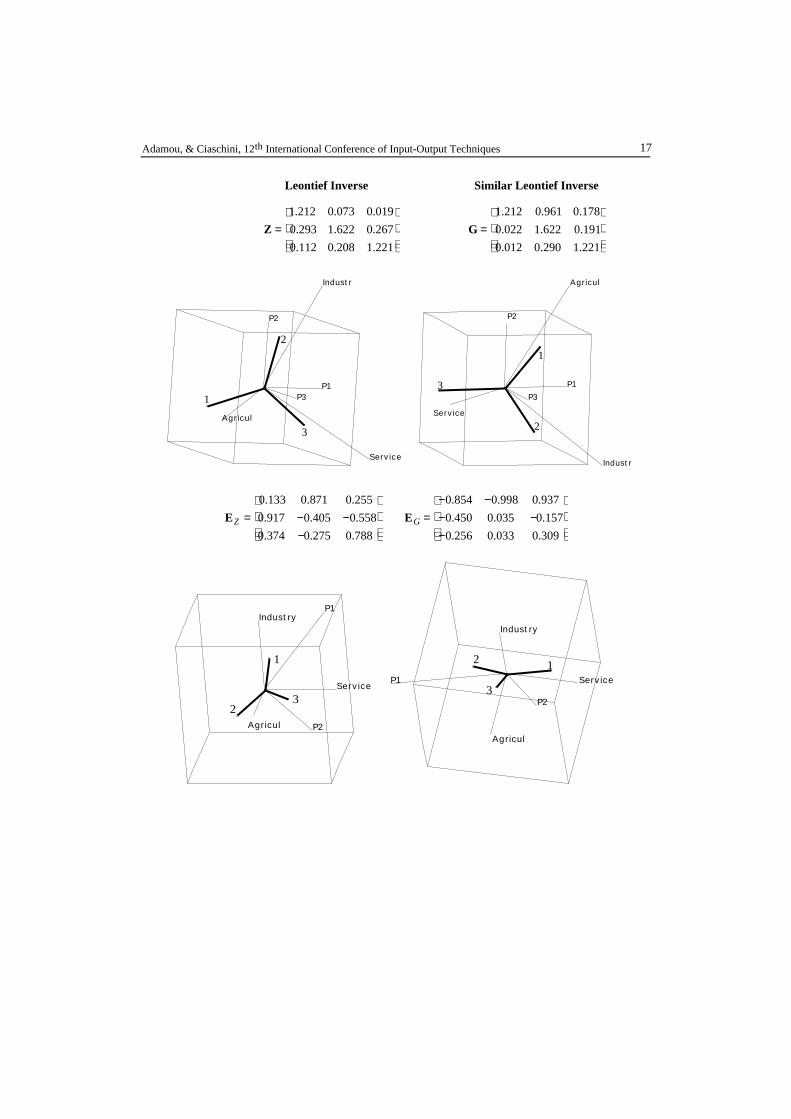
Leontief Inverse Similar Leontief Inverse
Z =1.212 0.073 0.019
0.293 1.622 0.267
0.112 0.208 1.221
G =1.212 0.961 0.178
0.022 1.622 0.191
0.012 0.290 1.221
Agricul
Industr
Service
P1
P2
P31
2
3
Agricul
Industr
Service
P1
P2
P3
1
2
3
EZ =0.133 0.871 0.255
0.917 −0.405 −0.558
0.374 −0.275 0.788
EG =−0.854 −0.998 0.937
−0.450 0.035 −0.157
−0.256 0.033 0.309
P1
P2
Service
Industry
Agricul
1
23
P1
P2
Service
Industry
Agricul
12
3

Singular & Characteristic Structures of Similar Multisectoral Systems18
Direct Interaction of Eigenvectors of the Leontief & its Similar Inverses
η = EZEG−1[ ] η =
−0.789 −0.490 2.974
0.273 −0.816 −3.054
0.242 −1.802 0.900
Agricul
Industr
Service
P1
P2
P3
3
2
1
Interaction of Eigenvectors of the Leontief & its Similar Inverses through Gross Output
µ = EZ−1diag x( )EG[ ] µ =
−4.663 0 0
0 −0.833 0
0 0 2.667
Agricul
Industr
Service
P1
P2P3
1
2
3

Adamou, & Ciaschini, 12th International Conference of Input-Output Techniques 19
V Z =−0.276 0.910 0.307
−0.878 −0.110 −0.464
−0.389 −0.398 0.830
VG =−0.644 −0.364 0.671
−0.707 −0.048 −0.705
−0.290 0.929 0.226
Agricul
Industr
Service
P1
P2
P3
1
3
2 Agricul
Industr
Service
P1
P2
P3 3
1
2
U ZT =
−0.353 −0.846 −0.396
0.886 −0.168 −0.430
0.298 −0.504 0.810
UGT =
−0.380 −0.879 −0.287
−0.373 −0.138 0.917
0.845 −0.456 0.275
Agricul
Industr
Service
P1
P2
P32
3
1
Agricul
Industr
Service
P1
P2
P32
3
1

Singular & Characteristic Structures of Similar Multisectoral Systems20
ζev = EZ−1V Z[ ] ζev
s = EG−1VG[ ]
ζev =−1.048 0.216 0.123
−0.143 1.079 0.037
−0.045 −0.230 1.007
ζev
s =1.441 −0.463 1.010
−0.314 2.926 −0.055
0.291 2.304 1.577
Agricul
Industr
ServiceP1
P2
P31
23
Agricul
Industr
Service
P1
P2
P3
12
3
ζeu = U ZT EZ[ ] ζev
s = EG−1VG[ ]
ζeu =−0.972 0.144 0.069
−0.197 0.959 −0.019
−0.119 0.240 0.997
ζev
s =1.441 −0.463 1.010
−0.314 2.926 −0.055
0.291 2.304 1.577
Agricul
Industr
Service
P1
P2P3 1
23
AgriculIndustr
Service
P1
P2P3
12
3
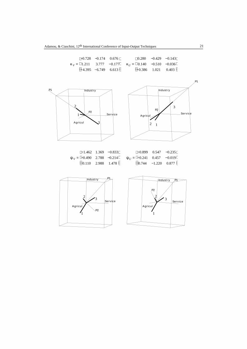
Adamou, & Ciaschini, 12th International Conference of Input-Output Techniques 21
κ V =−0.728 −0.174 0.676
1.211 3.777 −0.177
−4.395 −6.749 6.613
κU =0.280 −0.429 −0.143
0.140 −0.510 −0.036
−0.386 1.021 0.403
P1
P2Service
Industry
Agricul
1
2
3
P1
P2Service
Industry
Agricul
12
3
ψ V =−1.462 1.369 −0.833
−0.490 2.788 −0.214
0.110 2.988 1.478
ψU =−0.899 0.547 −0.235
−0.241 0.457 −0.019
0.744 −1.220 0.877
P1
P2
Service
Industry
Agricul
1
23
P1
P2
Service
Industry
Agricul
1
23

Singular & Characteristic Structures of Similar Multisectoral Systems22
Eigenvalues Diagonal of Gross Output
Principal ComponentsEigenValue:Percent:CumPercent:Eigenvectors:Column 1Column 2Column 3
1.5000 50.0000 50.0000
0.40825 0.40825-0.81650
1.5000 50.0000
100.0000
-0.70711 0.70711 0.00000
0.0000 0.0000
100.0000
0.57735 0.57735 0.57735
Principal ComponentsEigenValue:Percent:CumPercent:Eigenvectors:AgricultureIndustryServices
1.5000 50.0000 50.0000
-0.40825-0.40825 0.81650
1.5000 50.0000
100.0000
-0.70711 0.70711 0.00000
-0.0000 -0.0000
100.0000
0.57735 0.57735 0.57735
0.707 -1.225 0.000 -0.707 -1.225 0.0000.707 1.225 0.000 -0.707 1.225 0.000
-1.414 0.000 0.000 1.414 0.000 0.000
Singular Values of the Leontief Inverse Singular Values of the Similar Leontief Inverse
Principal ComponentsEigenValue:Percent:CumPercent:Eigenvectors:Column 1Column 2Column 3
1.5000 50.0000 50.0000
-0.70711 0.70711 0.00000
1.5000 50.0000
100.0000
0.40825 0.40825-0.81650
-0.0000 -0.0000
100.0000
0.57735 0.57735 0.57735
Principal ComponentsEigenValue:Percent:CumPercent:Eigenvectors:Column 1Column 2Column 3
1.5000 50.0000 50.0000
-0.70711 0.70711 0.00000
1.5000 50.0000
100.0000
0.40825 0.40825-0.81650
-0.0000 -0.0000
100.0000
0.57735 0.57735 0.57735
-1.225 0.707 0.000 -1.225 0.707 0.0001.225 0.707 0.000 1.225 0.707 0.0000.000 -1.414 0.000 0.000 -1.414 0.000
Leontief Inverse Similar Leontief Inverse
Principal ComponentsEigenValue:Percent:CumPercent:Eigenvectors:AgricultureIndustryServices
1.7944 59.8121 59.8121
-0.73499 0.20076 0.64768
1.2056 40.1879
100.0000
-0.15949 0.87719-0.45289
-0.0000 -0.0000
100.0000
0.65905 0.43617 0.61270
Principal ComponentsEigenValue:Percent:CumPercent:Eigenvectors:AgriculureIndustryServices
2.0102 67.0066 67.0066
0.36693 0.60656-0.70530
0.9898 32.9934
100.0000
0.85841-0.51294 0.00546
-0.0000 -0.0000
100.0000
0.35847 0.60744 0.70889
Eigenvectors of the Leontief Inverse Eigenvectors of the Similar Leontief Inverse
Principal ComponentsEigenValue:Percent:CumPercent:Eigenvectors:AgricultureIndustryServices
2.2104 73.6794 73.6794
-0.67259 0.53198 0.51441
0.7896 26.3206
100.0000
0.00985-0.68864 0.72504
0.0000 0.0000
100.0000
0.73995 0.49272 0.45793
Principal ComponentsEigenValue:Percent:CumPercent:Eigenvectors:AgricultureIndustryServices
2.7217 90.7237 90.7237
0.56768 0.60582-0.55742
0.2783 9.2763
100.0000
0.66455 0.06243 0.74463
-0.0000 -0.0000
100.0000
-0.48591 0.79315 0.36716
Copyright © 2022 FDOKUMEN