arX

iv:1

010.

3769

v1 [

astr

o-ph

.CO

] 1

9 O

ct 2

010

Chameleon dark energy models with characteristic signatures

Radouane Gannouji1,2, Bruno Moraes3, David F. Mota4, David Polarski3, Shinji Tsujikawa2, Hans A. Winther41IUCAA, Post Bag 4, Ganeshkhind, Pune 411 007, India

2Department of Physics, Faculty of Science, Tokyo University of Science,

1-3, Kagurazaka, Shinjuku-ku, Tokyo 162-8601, Japan3Lab. de Physique Theorique et Astroparticules, CNRS Universite Montpellier II, France and

4Institute of Theoretical Astrophysics University of Oslo, Norway

(Dated: October 20, 2010)

In chameleon dark energy models, local gravity constraints tend to rule out parameters in whichobservable cosmological signatures can be found. We study viable chameleon potentials consistentwith a number of recent observational and experimental bounds. A novel chameleon field potential,motivated by f(R) gravity, is constructed where observable cosmological signatures are present bothat the background evolution and in the growth-rate of the perturbations. We study the evolutionof matter density perturbations on low redshifts for this potential and show that the growth indextoday γ0 can have significant dispersion on scales relevant for large scale structures. The values of γ0can be even smaller than 0.2 with large variations of γ on very low redshifts for the model parametersconstrained by local gravity tests. This gives a possibility to clearly distinguish these chameleonmodels from the Λ-Cold-Dark-Matter (ΛCDM) model in future high-precision observations.

PACS numbers: 04.50.Kd, 95.36.+x

I. INTRODUCTION

The accelerated expansion of the Universe today is avery important challenge faced by cosmologists [1]. Foran isotropic comoving perfect fluid, a substantially nega-tive pressure is required to give rise to the cosmic accel-eration. One of the simplest candidates for dark energyis the cosmological constant with an equation of statewDE = −1, but we generally encounter a problem to ex-plain its tiny energy density consistent with observations[2].

There are alternative models of dark energy to thecosmological constant scenario. One of such models isquintessence based on a minimally coupled scalar fieldwith a self-interacting potential [3]. In order to realizethe cosmic acceleration today, the mass of quintessenceis required to be very small (mφ ≈ 10−33 GeV). From aviewpoint of particle physics, such a light scalar field maymediate a long range force with standard model particles[4]. For example, the string dilaton can lead to the vio-lation of equivalence principle through the coupling withbaryons [5]. In such cases we need to find some mecha-nism to suppress the fifth force for the consistency withlocal gravity experiments.

There are several different ways to screen the field in-teraction with baryons. One is the so-called run awaydilaton scenario [6] in which the field coupling F (φ)with the Ricci scalar R is assumed to approach a con-stant value as the dilaton φ grows in time (e.g., F (φ) =C1 + C2e

−φ as φ → ∞). Another way is to consider afield potential having a large mass in the region of highdensity where local gravity experiments are carried out.In this case the field does not propagate freely in the localregion, while on cosmological scales the field mass can belight enough to be responsible for dark energy.

The latter scenario is called the chameleon mechanism

in which a density-dependent matter coupling with thefield can allow the possibility to suppress an effective cou-pling between matter and the field outside a sphericallysymmetric body [7, 8]. The chameleon mechanism canbe applied to some scalar-tensor theories such as f(R)gravity [9, 10] and Brans-Dicke theory [11]. In f(R)gravity, for example, there have been a number of viabledark energy models [12] that can satisfy both cosmolog-ical and local gravity constraints. For such models thepotential of an effective scalar degree of freedom (called“scalaron” [13]) in the Einstein frame is designed to havea large mass in the region of high density. Even witha strong coupling between the scalaron and the baryons(Q = −1/

√6), the chameleon mechanism allows the f(R)

models to be consistent with local gravity constraints.

The chameleon models are a kind of coupledquintessence models [14] defined in the Einstein frame[7, 8]. While the gravitational action is described bythe usual Einstein-Hilbert action, non-relativistic mat-ter components are coupled to the Einstein frame metricmultiplied by some conformal factor which depends ona scalar (chameleon) field. This is how the gravitationalforce felt by matter is modified. While there have beenmany studies for experimental and observational aspectsof the chameleon models [15]-[38], it is not clear whichchameleon potentials are viable if the same field is to beresponsible for dark energy.

In this paper we identify a number of chameleon po-tentials that can be consistent with dark energy as well aslocal gravity experiments. We then constrain the viablemodel parameter space by using the recent experimentaland observational bounds– such as the 2006 Eot-Washexperiment [39], the Lunar Laser Ranging experiment[40] and the WMAP constraint on the time-variation ofparticle masses [41]. This can actually rule out some ofthe chameleon potentials with natural model parameters

2

for the matter coupling Q of the order of unity.In order to distinguish the viable chameleon dark en-

ergy models from the ΛCDM model, it is crucial to studyboth the modifications in the evolution of the backgroundcosmology and the modified evolution of the cosmologicaldensity perturbations. For the former, we shall considerthe evolution of the so-called statefinders introduced inRefs. [42, 43] and show that these parameters can exhibita peculiar behavior different from those in the ΛCDMmodel.On the other hand, the growth “index” γ of matter per-

turbations δm defined through d ln δm/d lna = (Ω∗m)γ ,

where a is a scale factor and Ω∗m is the density param-

eter of non-relativistic matter, is an important quantitythat allows to discriminate between different dark energymodels and interest in this quantity was revived in thecontext of dark energy models [44, 45].Its main importance for the study of dark energy mod-

els stems from the fact that for ΛCDM the quantity γ isknown to be nearly constant with respect to the red-shift z, i.e. γΛCDM = γ0 − 0.02z to exquisite accuracy[46], with γ0 ≡ γ(z = 0) ≈ 0.555 [44]. As emphasizedin Ref. [46], large variations of γ on low redshifts couldsignal that we are dealing with a dark energy model out-side General Relativity. This was indeed found for somescalar-tensor dark energy models [47] and f(R) models[48–50]. Such large variations can also occur in modelswhere dark energy interacts with matter [51, 52]. This isexactly the case in chameleon models, which we investi-gate in this paper, because of the direct coupling betweenthe chameleon field φ and all dust-like matter. This di-rect coupling is however not confined to the dark sectoras in standard coupled quintessence.An additional important point is the possible appear-

ance of a scale-dependence or dispersion in γ. Hencethe behavior of γ on low redshifts can be both time-dependent and scale-dependent [53–55]. This dispersioncan also be present in the models investigated here. Usingthe observations of large scale structure and weak lensingsurveys, one can hope to detect such peculiar behaviorsof γ (see e.g., Ref. [56]). If this is the case this would sig-nal that the gravitational law may be modified on scalesrelevant to large scale structures [45, 54, 55, 57–62].In this paper we study the evolution of γ as well as its

dispersion, its dependence on the wavenumbers of pertur-bations. We shall show that some of the chameleon mod-els investigated here can be clearly distinguished fromΛCDM through the behavior of γ exhibiting both largevariations and significant dispersion, with the possibilityto obtain small values of γ today as low as γ0 . 0.2.

II. CHAMELEON COSMOLOGY

A. Background equations

In this section we review the basic background evolu-tion of chameleon cosmology. We consider the chameleon

theory described by the following action [7, 8, 63]

S =

∫

d4x√−g

[

R

16πG− 1

2gµν∂µφ ∂νφ− V (φ)

]

+Sm

[

Ψm;A2(φ) gµν]

, (1)

where g is the determinant of the (Einstein frame) met-ric gµν , R is the Ricci scalar, G is the bare gravitationalconstant, φ is a scalar field with a potential V (φ), andSm is the matter action with matter fields Ψm. At lowredshifts it is sufficient to consider only non-relativisticmatter (cold dark matter and baryons), but for a gen-eral dynamical analysis including high redshifts radiationmust be included.We assume that non-relativistic matter is universally

coupled to the (Jordan frame) metric A2(φ) gµν , the Ein-stein frame metric gµν multiplied by a field-dependent(conformal) factor A2(φ). This direct coupling to thefield φ is how the gravitational interaction is modified.We can generalize this to arbitrary functions A(i)(φ) foreach matter component ρi, but in this work we will takethe same function A(φ) for all components. We write thefunction A(φ) in the form

A(φ) = eQφ/Mpl , (2)

where Mpl = 1/√8πG is the reduced Planck mass and Q

describes the strength of the coupling between the fieldφ and non-relativistic matter. In the following we shallconsider the case in which Q is constant. In fact, the con-stant coupling arises for Brans-Dicke theory by a confor-mal transformation to the Einstein frame [8, 11]. Evenwhen |Q| is of the order of unity, it is possible to makethe effective coupling between the field and matter smallthrough the chameleon mechanism.Let us consider the scalar field φ together with non-

relativistic matter (density ρ∗m) and radiation (densityρr) in a spatially flat Friedmann-Lemaıtre-Robertson-Walker (FLRW) space-time with a time-dependent scalefactor a(t) and a metric

ds2 = gµν dxµ dxν = −dt2 + a2(t) dx2 . (3)

The corresponding background equations are given by

3H2 = (ρφ + ρ∗m + ρr) /M2pl , (4)

φ+ 3Hφ+ V,φ = −Qρ∗m/Mpl , (5)

ρ∗m + 3Hρ∗m = Qρ∗mφ/Mpl , (6)

ρr + 4Hρr = 0 , (7)

where ρφ ≡ φ2/2 + V (φ), V,φ ≡ dV/dφ, and a dot rep-resents a derivative with respect to cosmic time t. Thequantity ρ∗m is the energy density of non-relativistic mat-ter in the Einstein frame and we have kept the star toavoid any confusion. Integration of Eq. (6) gives the so-lution ρ∗m ∝ a−3eQφ/Mpl . We define the conserved matterdensity:

ρm ≡ e−Qφ/Mplρ∗m , (8)

3

which satisfies the standard continuity equation, ρm +3Hρm = 0. Then the field equation (5) can be writtenin the form

φ+ 3Hφ+ Veff,φ = 0 , (9)

where Veff is the effective potential defined by

Veff ≡ V (φ) + eQφ/Mplρm . (10)

We emphasize that it is the Einstein frame which is thephysical frame. Due to the coupling between the fieldand matter, particle masses do evolve with time in ourmodel.We consider runaway positive potentials V (φ) in the

region φ > 0, which monotonically decrease and have apositive mass squared, i.e. V,φ < 0 and V,φφ > 0. Wealso demand the following conditions

limφ→0

∣

∣

∣

∣

V,φV

∣

∣

∣

∣

= ∞ , limφ→∞

V,φV

= 0 . (11)

The former is required to have a large mass in the regionof high density, whereas we need the latter condition torealize the late-time cosmic acceleration in the region oflow density. At φ = 0 the potential approaches either∞ or a finite positive value V0. In the limit φ → ∞ wehave either V → 0 or V → V∞, where V∞ is a nonzeropositive constant. If Q > 0 the effective potential Veff(φ)has a minimum at the field value φm (> 0) satisfying thecondition Veff,φ(φm) = 0, i.e.

V,φ(φm) +Q(ρm/Mpl)eQφm/Mpl = 0 . (12)

If the potential satisfies the conditions V,φ > 0 andV,φφ > 0 in the region φ < 0, there exists a minimum atφ = φm (< 0) provided that Q < 0. In fact this situationarises in the context of f(R) dark energy models [9, 10].Since the analysis in the latter is equivalent to that inthe former, we shall focus on the case Q > 0 and V,φ < 0in the following discussion.

B. Dynamical system

In order to discuss cosmological dynamics, it is conve-nient to introduce the following dimensionless variables

x1 ≡ φ√6HMpl

, x2 ≡√V√

3HMpl

, x3 ≡√ρr√

3HMpl

.

(13)Equation (4) expresses the constraint existing betweenthese variables, i.e.

Ω∗

m ≡ ρ∗m3H2M2

pl

= 1− Ωφ − Ωr , (14)

where

Ωφ ≡ x21 + x22 , Ωr ≡ x23 . (15)

Taking the time-derivative of Eq. (4) and making use ofEqs. (5)-(7), it is straightforward to derive the followingequation

H ′

H= −1

2

(

3 + 3x21 − 3x22 + x23)

, (16)

where a prime represents a derivative with respect toN ≡ ln a. A useful quantity is the effective equation ofstate

weff = −1− 2

3

H ′

H= x21 − x22 +

x233. (17)

We also introduce the field equation of state wφ, as

wφ ≡ φ2/2− V (φ)

φ2/2 + V (φ)=x21 − x22x21 + x22

. (18)

Using Eqs. (4)-(7), we obtain the following equations

x′1 = −3x1 +

√6

2λx22 − x1

H ′

H

−√6

2Q(

1− x21 − x22 − x23)

, (19)

x′2 = −√6

2λx1x2 − x2

H ′

H, (20)

x′3 = −2x3 − x3H ′

H, (21)

λ′ = −√6λ2(Γ− 1)x1 , (22)

where

λ ≡ −MplV,φV

, Γ ≡ V V,φφV 2,φ

. (23)

From the conditions (11) it follows that the quantity λdecreases from ∞ to 0 as φ grows from 0 to ∞. Sincex1 > 0 in Eq. (22), the condition λ′ < 0 translates into

Γ =V V,φφV 2,φ

> 1 . (24)

Chameleon potentials shallower than the exponential po-tential (Γ = 1) can satisfy this condition.Once the field settles down at the minimum of the ef-

fective potential (10), we have

x1 ≃ 0 , x2 ≃√

Q

λΩ∗

m , (25)

which gives wφ ≃ −1 from Eq. (18). As the matter den-sity ρ∗m decreases, the field evolves slowly along the in-stantaneous minima characterized by (25). We requirethat λ ≫ Q = O(1) during radiation and deep mattereras for consistency with local gravity constraints in theregion of high density. For the dynamical system (19)-(22) there is another fixed point called the “φ-matter-dominated era (φMDE)” [14] where Ωφ = weff = 2Q2/3.

4

However, since we are considering the case in which Q isof the order of unity, the effective equation of state weff istoo large to be compatible with observations. Only whenQ < O(0.1) the φMDE can be responsible for the matterera [14].When the chameleon is slow-rolling along the mini-

mum, we obtain the following relation from Eqs. (15)and (25):

λ

Q≃ Ω∗

m

Ωφ. (26)

While λ ≫ Q during the radiation and matter eras, λbecomes the same order as Q around the present epoch.The field potential is the dominant contribution on ther.h.s. of Eq. (4) today, so that

V (φ0) ≃ 3H20M

2pl ≃ ρc , (27)

where the subscript “0” represents present values andρc ≃ 10−29 g/cm3 is the critical density today.

III. CHAMELEON MECHANISM

In this section we review the chameleon mechanism asa way to escape local gravity constraints. In additionto the cosmological constraints discussed in the previ-ous section, this will enable us to restrict the forms ofchameleon potentials.Let us consider a spherically symmetric space-time in

the weak gravitational background with the neglect of thebackreaction of metric perturbations. As in the previoussection we consider the case in which couplingsQi are thesame for each matter component (Qi = Q), i.e., in whichthe function A(φ) is given by Eq. (2). Varying the action(1) with respect to φ in the Minkowski background, weobtain the field equation

d2φ

dr2+

2

r

dφ

dr=

dVeffdφ

, (28)

where r is the distance from the center of symmetry andVeff is defined in Eq. (10).Assuming that a spherically symmetric object (radius

rc and mass Mc) has a constant density ρm = ρA witha homogeneous density ρm = ρB outside the body, theeffective potential has two minima at φ = φA and φ = φBsatisfying the conditions

V,φ(φA) + Q(ρA/Mpl)eQφA/Mpl = 0 , (29)

V,φ(φB) + Q(ρB/Mpl)eQφB/Mpl = 0 . (30)

Since QφA/Mpl ≪ 1 and QφB/Mpl ≪ 1 for viable fieldpotentials in the regions of high density, the conservedmatter density ρm is practically indistinguishable fromthe matter density ρ∗m in the Einstein frame.The field profile inside and outside the body can be

found analytically. Originally this was derived in Refs. [7,

8] under the assumption that the field is frozen aroundφ = φA in the region 0 < r < r1, where r1 (< rc) is thedistance at which the field begins to evolve. It is possible,even without this assumption, to derive analytic solutionsby considering boundary conditions at the center of thebody [26].We consider the case in which the mass squared

m2B ≡ d2Veff

dφ2 (φB) outside the body satisfies the condi-

tion mBrc ≪ 1, so that the mB-dependent terms can benegligible when we match solutions at r = rc. The re-sulting field profile outside the body (r > rc) is given by[26]

φ(r) = φB − Qeff

4πMpl

Mc

r, (31)

where the effective coupling Qeff between the field andmatter is

Qeff = Q

[

1− r31r3c

+ 3r1rc

1

(mArc)2

×

mAr1(emAr1 + e−mAr1)

emAr1 − e−mAr1− 1

]

. (32)

The mass mA is defined by m2A ≡ d2Veff

dφ2 (φA).

The distance r1 is determined by the conditionm2

A [φ(r1)− φA] = QρA, which translates into

φB − φA +QρA(r21 − r2c )/(2Mpl)

=6QMplΦc

(mArc)2mAr1(e

mAr1 + e−mAr1)

emAr1 − e−mAr1, (33)

where Φc = Mc/(8πrc) = ρAr2c/(6M

2pl) is the gravita-

tional potential at the surface of the body.The fifth force exerting on a test particle of a unit mass

and a coupling Q is given by F = −Q∇φ/Mpl. UsingEq. (31), the amplitude of the fifth force in the regionr > rc is

F = 2 |QQeff |GMc

r2. (34)

As long as |Qeff | ≪ 1, it is possible to make the fifth forcesuppressed relative to the gravitational force GMc/r

2.From Eq. (32) the effective coupling Qeff can be mademuch smaller than Q provided that the conditions ∆rc ≡rc − r1 ≪ rc and mArc ≫ 1 are satisfied. Hence werequire that the body has a thin-shell and that the fieldis heavy inside the body for the chameleon mechanism towork.When the body has a thin-shell (∆rc ≪ rc), one can

expand Eq. (33) in terms of the small parameters ∆rc/rcand 1/(mArc). This leads to

ǫth ≡ φB − φA6QMplΦc

≃ ∆rcrc

+1

mArc, (35)

where ǫth is called the thin-shell parameter. As long asmArc ≫ (∆rc/rc)

−1, this recovers the relation ǫth ≃

5

∆rc/rc [7, 8]. The effective coupling (32) is approxi-mately given by

Qeff ≃ 3Qǫth . (36)

If ǫth is much smaller than 1 then one has Qeff ≪ Q,so that the models can be consistent with local gravityconstraints.As an example, let us consider the experimental bound

that comes from the solar system tests of the equiva-lence principle, namely the Lunar Laser Ranging (LLR)experiment, using the free-fall acceleration of the Moon(aMoon) and the Earth (a⊕) toward the Sun (mass M⊙)[8, 10, 26]. The experimental bound on the difference oftwo accelerations is given by

2|aMoon − a⊕|(aMoon + a⊕)

< 10−13 . (37)

Under the conditions that the Earth, the Sun, and theMoon have thin-shells, the field profiles outside the bod-ies are given as in Eq. (31) with the replacement of corre-sponding quantities. The acceleration induced by a fifthforce with the field profile φ(r) and the effective couplingQeff is afifth = |Qeff∇φ(r)/Mpl|. Using the thin-shell pa-rameter ǫth,⊕ for the Earth, the accelerations a⊕ andaMoon are [8]

a⊕ ≃ GM⊙

r2

[

1 + 18Q2ǫ2th,⊕Φ⊕

Φ⊙

]

, (38)

aMoon ≃ GM⊙

r2

[

1 + 18Q2ǫ2th,⊕Φ2

⊕

Φ⊙ΦMoon

]

, (39)

where Φ⊙ ≃ 2.1× 10−6, Φ⊕ ≃ 7.0× 10−10, and ΦMoon ≃3.1×10−11 are the gravitational potentials of Sun, Earthand Moon, respectively. Then the condition (37) reads

ǫth,⊕ <8.8× 10−7

Q. (40)

Using the value Φ⊕ ≃ 7.0× 10−10, the bound (40) trans-lates into

φB,⊕ . 10−15Mpl , (41)

where we used the condition φB,⊕ ≫ φA,⊕. For the Earthone has ρA ≃ 5 g/cm3(mean density of the Earth) ≫ρB ≃ 10−24 g/cm3 (dark matter/baryon density in ourgalaxy), so that the condition φB,⊕ ≫ φA,⊕ is satisfied.In Sec. IV we constrain viable chameleon potentials by

employing the condition (41) together with the cosmo-logical condition we discussed in Sec. II. In Sec. V werestrict the allowed model parameter space further byusing a number of recent local gravity and observationalconstraints.

IV. VIABLE CHAMELEON POTENTIALS

We now discuss the forms of viable field potentials thatcan be in principle consistent with both local gravity and

cosmological constraints. Let us consider the potential

V (φ) =M4f(φ) , (42)

where M is a mass scale and f(φ) is a dimensionlessfunction in terms of φ.The local gravity constraint coming from the LLR ex-

periment is given by Eq. (41), where φB,⊕ is determinedby solving

|Mplf,φ(φB,⊕)| ≃ QρB/M4 . (43)

Here we take ρB ≃ 10−24 g/cm3 for the homogeneousdensity outside the Earth. Once the form of f(φ) is spec-ified, the constraint on the model parameter, e.g.,M , canbe derived.From the cosmological constraint (26), λ/Q is of the

order of 1 today. Then it follows that

|Mplf,φ(φ0)| ≃ Qf(φ0) ≃ Qρc/M4 , (44)

where we used Eq. (27).We also require the condition (24), i.e.

Γ =ff,φφf2,φ

> 1 , (45)

for all positive values of φ. We shall proceed to find viablepotentials satisfying the conditions (41), (43), (44), and(45). From Eqs. (43) and (44) we obtain

f,φ(φB,⊕)

f,φ(φ0)≃ ρB

ρc≃ 105 . (46)

Let us consider the inverse power-law potential V (φ) =M4+nφ−n (n > 0), i.e.

f(φ) = (M/φ)n . (47)

Since Γ = (n+ 1)/n > 1, the condition (45) is automati-cally satisfied. The cosmological constraint (44) gives

φ0 ≃ nMpl/Q . (48)

From Eq. (46) we find the relation between φ0 and φB,⊕ :

φ0 ≃ 105/(n+1)φB,⊕ . (49)

Using the LLR bound (41), it follows that

φ0 . 10−5(3n+2)

n+1 Mpl . (50)

This is incompatible with the cosmological constraint(48) for n ≥ 1 and Q = O(1). Hence the inverse power-law potential is not viable.

A. Inverse power-law potential + constant

The reason why the inverse power-law potential doesnot work is that the field value today required for cosmic

6

acceleration is of the order ofMpl, while the local gravityconstraint demands a much smaller value. This problemcan be circumvented by taking into account a constantterm to the inverse power-law potential. Let us thenconsider the potential V (φ) = M4 [1 + µ(M/φ)n] (n >0), i.e.

f(φ) = 1 + µ(M/φ)n , (51)

where µ is a positive constant. The rescaling of the massterm M always allows to normalize the constant to beunity in Eq. (51). For this potential the quantity Γ reads

Γ =n+ 1

n

[

1 +1

µ

(

φ

M

)n]

, (52)

which satisfies the condition Γ > 1. In the regionµ(M/φ)n ≫ 1 we have that Γ ≃ (n+1)/n, which recoversthe case of the inverse power-law potential. Meanwhile,in the region µ(M/φ)n ≪ 1, one has Γ ≫ 1. The latterproperty comes from the fact that the potential becomesshallower as the field φ increases. This modification ofthe potential allows a possibility that the model can beconsistent with both cosmological and local gravity con-straints.The addition of a constant term to the inverse power-

law potential does not affect the condition (46), whichmeans that the resulting bounds (49) and (50) are notsubject to change. On the other hand, the cosmologi-cal constraint (48) is modified. Let us consider the casewhere the condition µ(M/φ0)

n ≪ 1 is satisfied today, i.e.f(φ0) ≃ 1. From Eq. (44) it follows that

M ≃ ρ1/4c ≃ 10−12GeV , (53)

and

φ0 ≃(

nµMn

Mnpl

)1/(n+1)

Mpl ≃ (10−30nnµ)1/(n+1)Mpl .

(54)Hence the field value φ0 today can be much smaller thanthe Planck mass, unlike the inverse power-law potential.From Eqs. (50) and (54) we get the constraint

µ . 1015n−10/n . (55)

If n = 1, for example, one has µ . 105. Forlarger n the bound on µ becomes even weaker. Wenote that the condition µ(M/φ)n < 1 is satisfied forφ/Mpl & 10−10/n−15/n1/n. This shows that even thefield value such as φB,⊕ = 10−15Mpl satisfies the con-dition µ(M/φB,⊕)

n < 1. Thus the term µ(M/φ)n issmaller than 1 for the field values we are interested in(φB,⊕ . φ . φ0).A large range of experimental bounds for this model

has been derived in the literature, see Refs. [8, 17, 20, 24].For Q = n = 1, it was found in Ref. [20] that the model isruled out by the Eot-Wash experiment unless µ . 10−5.This applies for general n: to obtain a viable model for

Q of the order of unity one must impose a fine-tuningn≫ 1 or µ≪ 1.The potentials, which have only one mass scale equiv-

alent to the dark energy scale, are usually strongly con-strained by the Eot-Wash experiment. We shall look intothis issue in more details in Sec. V.

B. Construction of viable chameleon potentials

relevant to dark energy

The discussion given above shows that a functionf(φ) that monotonically decreases without a constantterm is difficult to satisfy both cosmological and lo-cal gravity constraints. This is associated with thefact that for any power-law form of f(φ) the condition|Mplf,φ(φ0)/f(φ0)| ≃ 1 leads to the overall scaling of thefunction f(φ0) itself, giving φ0 of the order of Mpl. Thedominance of a constant term in f(φ0) changes this sit-uation, which allows a much smaller value of φ0 relativeto Mpl.Another example similar to V (φ) =M4[1 + µ(M/φ)n]

is the potential [15]

V (φ) =M4 exp[µ(M/φ)n] , (56)

where µ > 0 and n > 0. For this model the quantity

Γ = 1 +n+ 1

n

1

µ

(

φ

M

)n

, (57)

is larger than 1. In the asymptotic regimes characterizedby µ(M/φ)n ≫ 1 and µ(M/φ)n ≪ 1 we have Γ ≃ 1 andΓ ≫ 1, respectively. When µ(M/φ)n ≪ 1 the functionf(φ) = exp[µ(M/φ)n] can be approximated as f(φ) ≃1+µ(M/φ)n, which corresponds to Eq. (51). In this casethe constraints on the model parameters are the same asthose given in Eqs. (53)-(55).There is another class of potentials that behaves as

V (φ) ≃ M4[1 − µ(φ/M)n] (µ > 0, 0 < n < 1) in the re-gion µ(φ/M)n ≪ 1. In fact this asymptotic form corre-sponds to the potential that appears in f(R) dark energymodels. While the potential is finite at φ = 0 the deriva-tive |V,φ| diverges as φ → 0 for 0 < n < 1, so that thefirst of the condition (11) is satisfied. In order to keepthe potential positive we need some modification of V inthe region µ(φ/M)n > 1.In scalar-tensor theory it was shown in Ref. [11] that

the Jordan frame potential of the form U(φ) = M4[1 −µ(1 − e−2Qφ/Mpl)n] (0 < µ < 1, 0 < n < 1) can satisfyboth cosmological and local gravity constraints. In thiscase the potential V (φ) in the Einstein frame is givenby V (φ) = e4Qφ/MplU(φ), which possesses a de Sitterminimum due to the presence of the conformal factor.Cosmologically the solutions finally approach the de Sit-ter fixed point, so that the late-time cosmic accelerationcan be realized.Now we would like to consider a runaway positive po-

tential in the Einstein frame. One example is

V (φ) =M4[1− µ(1− e−φ/Mpl)n] , (58)

7

0 1 2 3 40.2

0.4

0.6

0.8

1.0

ΦMPl

VM

4

FIG. 1: The potential (58) versus the field φ for µ = 0.7 andn = 0.7. The potential has a finite value V = M4 at φ = 0,but its derivatives diverge (|V,φ| → ∞ and V,φφ → ∞) asφ → 0.

where 0 < µ < 1 and 0 < n < 1. This potential be-haves as V (φ) ≃ M4[1 − µ(φ/Mpl)

n] for φ ≪ Mpl andapproaches V (φ) →M4(1−µ) in the limit φ≫Mpl (seeFig. 1). For the potential (58) we obtain

Γ− 1 =1− nx− µ(1− x)n

nµx(1 − x)n, x ≡ e−φ/Mpl . (59)

One can easily show that the r.h.s. is positive under theconditions 0 < µ < 1, 0 < n < 1, so that Γ > 1. In bothlimits φ → 0 and φ → ∞ one has Γ → +∞. Since Γ hasa minimum at a finite field value, the condition Γ ≫ 1 isnot necessarily satisfied today (unlike the potential (56)).

Unless µ is very close to 1 the potential energy todayis roughly of the order of M4, i.e. f(φ0) ≈ 1. FromEq. (44) it then follows that

nµ(1− x0)n−1x0 ≃ Q , (60)

where x0 ≡ e−φ0/Mpl . If φ0 ≪ Mpl, we have that

φ0/Mpl ≃ (nµ)1/(1−n). From Eq. (43) we obtain

nµ(1− xB)n−1xB ≃ 105Q , (61)

where xB ≡ e−φB/Mpl . Under the condition φB ≪ Mpl

we have φB/Mpl ≃ (10−5nµ/Q)1/(1−n) from Eq. (61).Then the LLR bound (41) corresponds to

n · 1010−15n < Q/µ . (62)

When µ = 0.5 and µ = 0.05 with Q = 1, the constraint(62) gives n & 0.63 and n & 0.56 respectively.

C. Statefinder analysis

The statefinder diagnostics introduced in Refs. [42, 43]can be a useful tool to distinguish dark energy modelsfrom the ΛCDM model. The statefinder parameters aredefined by

r =

...a

aH3, s =

r − 1

3(q − 1/2), (63)

where q ≡ −a/(aH2) is the deceleration parameter.Defining h ≡ H2, it follows that

q = −1− h′

2h, r = 1 +

h′′

2h+

3h′

2h, (64)

where a prime represents a derivative with respect toN = ln a.In the radiation dominated epoch we have h ∝ e−4N ,

which gives (r, s) ≃ (3, 4/3). During the matter era r ap-proaches 1, whereas s blows up from positive to negativebecause of the divergence of the denominator in s (i.e.q = 1/2). For the chameleon potentials (56) and (58)the solutions finally approach the de Sitter fixed pointcharacterized by (r, s) = (1, 0). Around the de Sitterpoint the solutions evolve along the instantaneous min-ima characterized by (x1, x2, x3) = (λ/

√6,√

1− λ2/6, 0)with h ∝ V . Using Eq. (22) as well, one has h′/h ≃ −λ2and h′′/h ≃ (2Γ− 1)λ4. Then the statefinder diagnosticsaround the de Sitter point can be estimated as

r ≃ 1 +

(

Γ− 1

2

)

λ4 − 3

2λ2 , (65)

s ≃ − (2Γ− 1)λ4 − 3λ2

3(3− λ2). (66)

Since λ finally approaches 0, Eq. (22) implies thatΓλ3 → 0 asymptotically. For the potential in whichΓ ≫ 1 holds today it can happen that Γλ4 ≫ λ2, whichgives r ≃ 1 + Γλ4 > 1 and s ≃ −2Γλ4/[3(3 − λ2)] < 0around the present epoch. In the upper panel of Fig. 2we plot the evolution of the variables r and s for the po-tential (56) in the redshift regime −1 < z ≡ 1/a−1 < 10.The statefinders evolve toward the de Sitter point char-acterized by (r, s) = (1, 0) from the regime r > 1 ands < 0. This behavior is different from quintessence withthe power-law potential V (φ) = M4+nφ−n (n > 0) inwhich the statefinders are confined in the region r < 1and s > 0 [42, 43].The potential (58) allows the possibility that Γ is not

much larger than 1 even at the present epoch. In theregime λ2 ≪ 1 we then have r ≃ 1 − 3λ2/2 < 1 ands ≃ λ2/3 > 0. In fact we have numerically confirmedthat the solutions enter this regime by today (see thelower panel of Fig. 2). Finally they approach the de Sitterpoint from the regime r < 1 and s > 0. Hence onecan distinguish between chameleon potentials from theevolution of statefinders.

8

z=10

z=5

z=-1

-2.5 -2.0 -1.5 -1.0 -0.5 0.0

1.000

1.002

1.004

1.006

1.008

s

r

z=10

z=-0.999

z=0

-0.05 0.00 0.05 0.10 0.150.5

0.6

0.7

0.8

0.9

1.0

s

r

FIG. 2: (Top): Evolution of the statefinders r and s for thepotential (56) with n = 1, Q = 1 and µ = 1. The solutionsapproach the de Sitter point at (r, s) = (1, 0) from the regionr > 1 and s < 0. (Bottom): Evolution of statefinders for thepotential (58) with n = 0.7, Q = 1 and µ = 0.7. In this casethe solutions approach the de Sitter point from the regionr < 1 and s > 0.

V. LOCAL GRAVITY CONSTRAINTS ON

CHAMELEON POTENTIALS

In this section we discuss a number of local gravityconstraints on the chameleon potentials (56) and (58) indetails. Together with the LLR bound (41) we use theconstraint coming from 2006 Eot-Wash experiments [39]as well as the WMAP bound on the variation of the field-dependent mass.

A. The WMAP constraint on the variation of the

particle mass

Due to the conformal coupling of the field φ to matter,any particle will acquire a φ-dependent mass:

m(φ) = m0eQφ/Mpl , (67)

where m0 is a constant.The WMAP data constrain any variation in m(φ), be-

tween now and the epoch of recombination to be . 5%at 2σ (. 23% at 4σ) [41]. We then require that

∣

∣

∣

∣

∆m(φ)

m

∣

∣

∣

∣

=

∣

∣

∣

∣

eQ(φ0−φrec)

Mpl − 1

∣

∣

∣

∣

. 0.05 , (68)

where φrec is the field value at the recombination epoch.If we assume that the chameleon follows the minimumsince recombination then φ0 ≫ φrec, and the field in thecosmological background today must satisfy

Qφ0/Mpl . 0.05 . (69)

This provides a constraint on the coupling Q and themodel parameters of chameleon potentials.Note that the WMAP constraint is not a local gravity

constraint. Nevertheless, it provides strong constraintson the potential (58) with natural parameters and istherefore considered in this section.

B. Constraints from the 2006 Eot-Wash

experiment

The 2006 Eot-Wash experiment [39] searched for de-viations from the 1/r2 force law of gravity. The experi-ment used two parallel plates, the detector and attractor,which are separated by a (smallest) distance d = 55µm.The plates have holes of different sizes bored into them,and the attractor is rotating with an angular velocity ω.The rotation of the attractor gives rise to a torque on thedetector, and the setup of the experiment is such that thistorque vanishes for any force that falls off as 1/r2. In be-tween the plates there is a ds = 10µm BeCu-sheet, whichis for shielding the detector from electrostatic forces.The chameleon force between two parallel plates, see

e.g. Ref. [24], usually falls off faster than 1/r2, imply-ing a strong signature on the experiment. However, ifthe matter-coupling is strong enough, the electrostaticshield will itself develop a thin-shell. When this hap-pens, the effect of this shield is not only to shield elec-trostatic forces, but also to shield the chameleon force onthe detector. This suppression is approximately given bya factor exp(−msds), where ms is the mass inside theelectrostatic shield. Hence the experiment cannot detectstrongly coupled chameleons.The behavior of chameleons in the Eot-Wash experi-

ment have been explained in Refs. [20, 27, 38]. We calcu-late the Eot-Wash constraints on our models numericallybased on the prescription presented in Ref. [27].

9

FIG. 3: The combined local gravity constraints on the poten-tial (56) with µ = 1 in the (n,Q) plane. The shaded regioncorresponds to the allowed parameter space. The natural val-ues of Q and n of the order of unity are excluded.

C. Combined local gravity constraints

1. Potential V (φ) = M4 exp[µ(M/φ)n]

Let us first consider the inverse-power law potential(56) with n > 0. From Eq. (12) the field value φm at theminimum of the effective potential Veff satisfies

(

M

φm

)n+1

=Q

µn

M

Mpl

ρmeQφm/Mpl

V (φm). (70)

In this model the field is in the regime M ≪ φm ≪ Mpl

for the density ρm we are interested in. Since V (φm) canbe approximated as V (φm) ≃M4, it follows that

φmM

≃(

Q

µn

M

Mpl

ρmM4

)−1/(n+1)

. (71)

Using the LLR bound (41) with the homogeneous den-sity ρm ≃ 10−24 g/cm3 in our galaxy, we obtain the con-straint

n · 1010−15n < Q/µ . (72)

The WMAP bound (69) gives

Q <Mpl

M

(

0.05n+1

µn

ρ(0)m

M4

)1/n

, (73)

where ρ(0)m is the matter density today, with ρ

(0)m /M4 ≈

Ω∗(0)m /Ω

(0)φ ≈ 1/3. Since Mpl/M ≈ 1030, this condition is

well satisfied for Q,n, µ of the order of unity.

For the Eot-Wash experiment, the chameleon torqueon the detector was found numerically to be larger thanthe experimental bound when Q,n, µ are of the order ofunity. Providing the electrostatic shield with a thin-shell,we require that n ≫ 1, Q ≫ 1 or µ ≪ 1 to satisfy theexperimental bound.In Fig. 3 we plot the region constrained by the bounds

(72), (73), and the Eot-Wash experiment for µ = 1. Thisshows that only the large coupling region with Q≫ 1 canbe allowed for n of the order of unity. A viable model canalso be constructed by taking values of µ much smallerthan 1. Note that the WMAP bound (73) is satisfied forthe parameter regime shown in Fig. 3.

2. Potential V (φ) = M4[1− µ(1− e−φ/Mpl)n]

Let us proceed to another potential (58) with 0 < n <1. In the regions of high density where local gravity ex-periments are carried out, we have φ ≪ Mpl and henceV (φ) ≃ M4[1 − µ(φ/Mpl)

n]. In this regime the effectivepotential Veff has a minimum at

φm =

(

Q

µn

ρmM4

)1/(n−1)

Mpl . (74)

Recall that the LLR bound was already derived inEq. (62), which is the same as the constraint (72) of theprevious potential.Assuming that the chameleon is at the minimum of its

effective potential in the cosmological background today,the WMAP bound (69) translates into

Q & 0.05(60nµ)1/n , (75)

where we have used ρ(0)m /M4 ≈ 1/3 in Eq. (74). However,

a full numerical simulation of the background evolutionshows that this is not always the case. For a large rangeof parameters the chameleon has started to lag behindthe minimum, which again leads to a weaker constraint.The Eot-Wash experiment provides the strongest con-

straints when Q is of the order of unity for the potentials(51) and (56). This is not the case for the potential (58),because the electrostatic shield used in the experimentdevelops a thin-shell.The mass inside the electrostatic shield is given by

m2s ≃ n(1− n)µ

(

QρsµnM4

)

2−n1−n M4

M2pl

. (76)

Using ρs ≃ 10 g/cm3 and ds ≃ 10µm we have

msds ≃√

n(1− n)µ

(

Q

µn

)

2−n1−n

106−35n1−n . (77)

Taking Q and µ to be of the order of unity, we findmsds ≫ 1 as long as n & 0.2. The suppression of thechameleon torque due to the presence of the electrostaticshield makes the chameleon invisible in the experiment.

10

FIG. 4: The combined local gravity constraints on the poten-tial (58) with µ = 0.5 in the (n,Q) plane. In this case theallowed parameter space (shaded region in the figure) is de-termined by the WMAP constraint and the LLR constraint.

FIG. 5: The combined local gravity constraints on the po-tential (58) with µ = 0.05. The allowed parameter space isdetermined by the LLR bound. The WMAP constraint issatisfied for the whole parameter space in the figure.

In Figs. 4 and 5 we plot the allowed regions constrainedby the bounds (62), (75), and the Eot-Wash experiments,for µ = 0.5 and µ = 0.05, respectively. When µ = 0.5 theWMAP constraint gives the tightest bound for Q & 0.2,and the parameter spaceQ . 1 is viable for n & 0.7. If wedecrease the values of µ down to 0.05, then the WMAPbound is well satisfied for the parameter space shown inFig. 5. Instead, the LLR experiment provides the tightestbound in such cases. When µ = 0.05, the region with0.1 . Q . 10 and n & 0.6 can be allowed. The coupling

Q as well as the parameter n are not severely constrainedfor the potential (58).

VI. LINEAR GROWTH OF MATTER

PERTURBATIONS

We now turn our attention to cosmological perturba-tions in chameleon cosmology. It is well-known that mat-ter perturbations allow to discriminate between dark en-ergy models where the gravitational interaction is mod-ified on cosmic scales. We first review the general for-malism and derive the equation for linear matter pertur-bations. We also introduce important quantities like thecritical scale λc below which modifications of gravity arefelt and the growth index γ(z, k), a powerful discrimina-tive quantity for the study of the modified evolution ofmatter perturbations as was explained in the Introduc-tion.As we have seen in Sec. V, local gravity constraints im-

pose very strong boundaries on the potential (56), forc-ing its parameters to take unnatural values. Moreover,for viable choices of parameters, we have verified thatthe linear perturbations behave in a manner similar tothe ΛCDM model, as λc is much smaller than the cosmicscales we are interested in. On the other hand we haveshown that the model parameters of the potential (58)is not severely constrained. In Sec. VIB we will showthat the potential (58) gives rise to some very interestingobservational signatures.

A. General formalism for cosmological

perturbations

We consider scalar metric perturbations α, B, ψ, andγ around a flat FLRW background. The line-elementdescribing such a perturbed Universe is given by [64]

ds2 = −(1 + 2α)dt2 − 2aB,idtdxi

+a(t)2 [(1 + 2ψ)δij + 2γ,i;j] dxidxj . (78)

We decompose the field φ into the background and inho-mogeneous parts: φ(t,x) = φ(t) + δφ(t,x). The energy-

momentum tensors T(m)µν of non-relativistic matter can

be decomposed as

T 00(m)

= −(ρ∗m + δρ∗m) , T 0i(m)

= −ρ∗mv,i , (79)

where v is the peculiar velocity potential of non-relativistic matter. In the following, when we expressbackground quantities, we drop the tilde for simplicity.Let us consider the evolution of matter perturbations,

δm ≡ δρ∗m/ρ∗m in the comoving gauge (v = 0). The quan-

tity δm corresponds to the gauge-invariant quantity in-troduced in Refs. [64–66] when expressed in the comovinggauge. In the Fourier space the first-order perturbationequations are given by [67, 68]

11

α = −Qδφ/Mpl , (80)

˙δρ∗m + 3Hδρ∗m − ρ∗m (κ− 3Hα)−Q(ρ∗m˙δφ+ δρ∗mφ)/Mpl = 0 , (81)

δφ+ 3H ˙δφ+

(

V,φφ +k2

a2

)

δφ+ 2αV,φ − φ(α− 3Hα+ κ) +Q(2αρ∗m + δρ∗m)/Mpl = 0 , (82)

κ+ 2Hκ+ 3Hα− k2

a2α− 1

2M2pl

(

δρ∗m − 4αφ2 + 4φ ˙δφ− 2V,φδφ)

= 0 , (83)

where k is a comoving wavenumber and κ ≡ 3(Hα− ψ)+(k2/a)(B + aγ). From Eq. (81) it follows that

κ = δm −Q( ˙δφ+ 3Hδφ)/Mpl , (84)

where we have used Eq. (80). Plugging Eq. (84) intoEqs. (82) and (83), we obtain

δφ+

(

3H + 2Qφ

Mpl

)

˙δφ+

(

m2φ +

k2

a2− 2Q

V,φMpl

− 2Q2 ρ∗m

M2pl

)

δφ+Q

Mplρ∗mδm − φ δm = 0 , (85)

δm +

(

2H −Qφ

Mpl

)

δm − ρ∗mδm2M2

pl

(1− 2Q2) +

[

V,φM2

pl

+Q

Mpl

(

m2φ +

2k2

a2− 6H2 − 6H − 2φ2

M2pl

−2QV,φMpl

− 2Q2 ρ∗m

M2pl

)]

δφ+1

Mpl

(

2Q2 φ

Mpl− 2φ

Mpl− 2QH

)

˙δφ = 0 , (86)

where m2φ = V,φφ is the mass squared of the chameleon

field.As long as the field φ evolves slowly (“adiabatically”)

along the instantaneous minima of the effective potentialVeff , one can employ the quasi-static approximation onsub-horizon scales (k ≫ aH) [65, 66, 69]. This corre-sponds to the approximation under which the dominantterms in Eqs. (85) and (86) are those including k2/a2,mφ, and δm, i.e.

(

m2φ +

k2

a2

)

δφ ≃ − Q

Mplρ∗mδm , (87)

δm + 2Hδm − ρ∗mδm2M2

pl

(1 − 2Q2)

+Q

Mpl

(

m2φ +

2k2

a2

)

δφ ≃ 0 , (88)

where we have also used the approximation φ/Mpl ≪ H .Combining these equations, it follows that

δm + 2Hδm − 4πGeffρ∗

mδm ≃ 0 , (89)

where the effective gravitational coupling is given by

Geff = G

(

1 + 2Q2 k2/a2

m2φ + k2/a2

)

. (90)

An analogous modified equation was found in Refs. [11,66, 70], the crucial point being to elucidate the physi-cal significance of Geff . We can understand the physi-cal content of the modification of gravity by looking atthe corresponding gravitational potential in real space.The gravitational potential (per unit mass) is of the typeV (r) = −(G/r)

(

1 + 2Q2 e−mφr)

[71].

When we solve the full system of perturbations (86),we can, for some of our models, get a small discrepancycompared to (89). This can result in a non-negligible dif-ference of up to around 5% in the numerical calculationof the growth rate of matter perturbations. This arisesmainly because the field φ does not move exactly alongthe minimum of the effective potential but is instead lag-ging a little behind it.

We see that in chameleon models Geff is a scale-dependent as well as a time-dependent quantity. Clearlythe scale-dependent driving force in Eq. (90) induces inturn a scale dependence in the growth of matter pertur-bations with two asymptotic regimes, i.e.

Geff = G(1 + 2Q2) k/a≫ mφ or λ≪ λc , (91)

= G k/a≪ mφ or λ≫ λc , (92)

where we have introduced the physical wavelength λ =(2π/k)a. We have in particular λ0 = 2π/k today (a = 1).

12

The characteristic (physical) scale λc is defined by

λc = 2π/mφ . (93)

On scales λ ≫ λc matter perturbations do not feel thefifth force during their growth. On the contrary, on scalesmuch smaller than λc they do feel its presence. Duringthe matter dominance (Ω∗

m ≃ 1) the solutions to Eq. (89)are given by

δm ∝ a[√

1+24(1+2Q2)−1]/4 λ≪ λc , (94)

δm ∝ a λ≫ λc . (95)

Hence, in the regime λ≪ λc, the growth rate gets largerthan that in standard General Relativity.As mentioned earlier, a powerful way to describe the

growth of perturbations is by introducing the functionγ(k, z) defined as follows

f = Ω∗

m(z)γ(k,z) , (96)

where

f =d ln δmd ln a

. (97)

We remind the definition δm ≡ δρ∗m/ρ∗m. The quantity

γ can be time-dependent and also scale-dependent. Itis known that a large class of dark energy models in-side General Relativity yields a quasi-constant γ withvalues close to that of the ΛCDM model, γ ≈ 0.55[45, 46]. Therefore any significant deviation from thisbehavior would give rise to a characteristic signature forour chameleon models. Since 0 < Ω∗

m(z) < 1, smaller γimplies a larger growth rate of matter perturbations.As we have seen before, the chameleon mechanism is

devised so that in high-density environments the mass ofthe scalar field is large relative to its value in low-densityones. During the cosmological evolution, the mass of thefield will follow this behavior, which means that λc willmove from small to large values. In other words, Geff

will evolve from the regime (92) to the regime (91). Thistransition is scale-dependent, which is an important fea-ture of the growth of matter perturbations in chameleon(and f(R)) models.We consider the evolution of matter perturbations for

the wavenumbers

0.01 hMpc−1 . k . 0.2 hMpc−1 , (98)

where h describes the uncertainty of the Hubble param-eter H0 today, i.e. H0 = 100 hkm sec−1 Mpc−1. Thescales (98) range from the upper limit of observable scalesin the linear regime of perturbations to the mildly non-linear regime (in which the linear approximation is stillreasonable).Depending on the value of λc today (denoted as λc,0)

and on its recent evolution, three possibilities can actu-ally arise: (i) The model is hardly distinguishable fromΛCDM; (ii) The model is distinguishable from ΛCDM

but shows no dispersion i.e. no scale-dependence. Inthis case low values of γ0 will also yield large slopesγ′0 ≡ (dγ/dz)(z = 0), much larger than in ΛCDM; andfinally (iii) The model is distinguishable from ΛCDM andshows some dispersion altogether. These three cases canbe characterized using the quantity γ0 ≡ γ(z = 0). Thisclassification is analogous to what was done for some vi-able f(R) models [54] and it can be defined as follows:

• (i) The region in parameter space for which γ0 >0.53 for all the scales described by (98). In thisregion γ′0 is small and γ is nearly constant.

• (ii) The region where γ0 is degenerate, i.e. as-sumes the same value for all the scales, with a valuesmaller than 0.5. In this region γ′0 is large and thereis a significant variation of γ.

• (iii) The region where γ0 shows some dispersion,i.e. a scale-dependence. For low γ0, γ

′0 is large and

we have significant changes of γ.

Models in the regions (ii) and (iii) can be clearly discrim-inated from ΛCDM. Some examples are shown in Figs. 6and 7. We investigate below in more details the appear-ance of these characteristic signatures.

B. Observational signatures in the growth of

matter perturbations

The main question when looking at linear perturba-tions in chameleon models is the order of magnitude ofthe scale λc. If the chameleon mass mφ is large such thatλc is less than the order of the galactic size, matter per-turbations on the scales relevant to large scale structuresdo not feel the chameleon’s presence. This is actuallythe case for the inverse power exponential potential (56)with model parameters bounded by observational andlocal gravity constraints. Therefore, we will concentratethe analysis of the perturbations on the potential (58).In the regime φ/Mpl ≪ 1 one can employ the approxi-

mation V (φ) ≃M4[1−µ(φ/Mpl)n]. In fact this approxi-

mation is valid for most of the cosmological evolution bytoday. Then we obtain the field mass at the minimum ofthe effective potential Veff(φ):

mφ ≃ 2π

λc,0e−

3(2−n)2(1−n)

N , (99)

where λc,0 is the critical length today, given by

λc,0 =2π

√

µn(1− n)

Mpl

M2

(

Q

µn

ρ(0)m

M4

)−2−n

2(1−n)

. (100)

Using the relation ρ(0)DE = 3M2

plH20Ω

(0)DE ≃ M4, we find

that λc,0 is at most of the order of H−10 . If Q = 1,

n = 0.6, µ = 0.05, and Ω(0)DE = 0.72, for example, λc,0 ≈

0.4H−10 . For the modes deep inside the Hubble radius

13

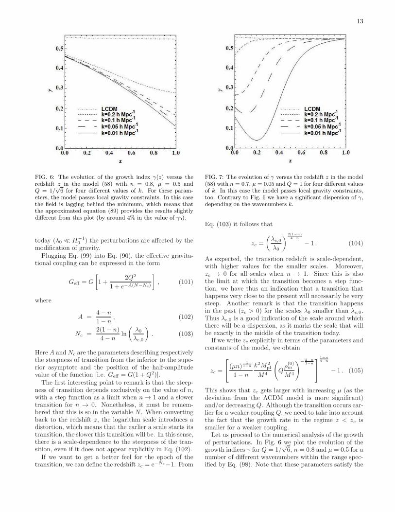
FIG. 6: The evolution of the growth index γ(z) versus theredshift z in the model (58) with n = 0.8, µ = 0.5 andQ = 1/

√6 for four different values of k. For these param-

eters, the model passes local gravity constraints. In this casethe field is lagging behind the minimum, which means thatthe approximated equation (89) provides the results slightlydifferent from this plot (by around 4% in the value of γ0).

today (λ0 ≪ H−10 ) the perturbations are affected by the

modification of gravity.Plugging Eq. (99) into Eq. (90), the effective gravita-

tional coupling can be expressed in the form

Geff = G

[

1 +2Q2

1 + e−A(N−Nc)

]

, (101)

where

A =4− n

1− n, (102)

Nc =2(1− n)

4− nln

(

λ0λc,0

)

. (103)

Here A andNc are the parameters describing respectivelythe steepness of transition from the inferior to the supe-rior asymptote and the position of the half-amplitudevalue of the function [i.e. Geff = G(1 +Q2)].The first interesting point to remark is that the steep-

ness of transition depends exclusively on the value of n,with a step function as a limit when n→ 1 and a slowertransition for n → 0. Nonetheless, it must be remem-bered that this is so in the variable N . When convertingback to the redshift z, the logarithm scale introduces adistortion, which means that the earlier a scale starts itstransition, the slower this transition will be. In this sense,there is a scale-dependence to the steepness of the tran-sition, even if it does not appear explicitly in Eq. (102).If we want to get a better feel for the epoch of the

transition, we can define the redshift zc = e−Nc−1. From

FIG. 7: The evolution of γ versus the redshift z in the model(58) with n = 0.7, µ = 0.05 and Q = 1 for four different valuesof k. In this case the model passes local gravity constraints,too. Contrary to Fig. 6 we have a significant dispersion of γ,depending on the wavenumbers k.

Eq. (103) it follows that

zc =

(

λc,0λ0

)

2(1−n)4−n

− 1 . (104)

As expected, the transition redshift is scale-dependent,with higher values for the smaller scales. Moreover,zc → 0 for all scales when n → 1. Since this is alsothe limit at which the transition becomes a step func-tion, we have thus an indication that a transition thathappens very close to the present will necessarily be verysteep. Another remark is that the transition happensin the past (zc > 0) for the scales λ0 smaller than λc,0.Thus λc,0 is a good indication of the scale around whichthere will be a dispersion, as it marks the scale that willbe exactly in the middle of the transition today.If we write zc explicitly in terms of the parameters and

constants of the model, we obtain

zc =

(µn)1

1−n

1− n

k2M2pl

M4

(

Qρ(0)m

M4

)−2−n1−n

1−n4−n

− 1 . (105)

This shows that zc gets larger with increasing µ (as thedeviation from the ΛCDM model is more significant)and/or decreasingQ. Although the transition occurs ear-lier for a weaker coupling Q, we need to take into accountthe fact that the growth rate in the regime z < zc issmaller for a weaker coupling.Let us proceed to the numerical analysis of the growth

of perturbations. In Fig. 6 we plot the evolution of thegrowth indices γ for Q = 1/

√6, n = 0.8 and µ = 0.5 for a

number of different wavenumbers within the range spec-ified by Eq. (98). Note that these parameters satisfy the

14

FIG. 8: The regions (i), (ii) and (iii) in the (n,µ) space forQ = 1/

√6 (top) and for Q = 1 (bottom). In the region (i) all

the modes have γ0 > 0.53. In region (ii) γ0 is degenerate withthe value smaller than 0.5, and finally (iii) shows the regimewhere γ0 is dispersed. It is clear that, for both choices of Q,there are viable choices of parameters in which the deviationfrom the ΛCDM model is present.

local gravity constraints discussed in Sec. V, see Fig. 4.At the present epoch these modes are in the regime (ii),with very similar growth indices today (γ0 ≃ 0.46). Asestimated by Eq. (105) the transition redshift zc is largerthan the order of 1 for k & 0.05 hMpc−1, e.g. zc = 2.3for k = 0.1 hMpc−1. The degenerate behavior similar tothat shown in Fig. 6 has been also found in some f(R)models [48, 54]. Numerically we have verified that valuesof γ0 in this case are slightly higher than those expectedin the asymptotic regime (λ ≪ λc). This discrepancycomes from the fact that the chameleon field is laggingbehind the minimum of the potential for this choice of

parameters. As a result, we need to solve the full per-turbation equations (85) and (86) instead of the approx-imated equation (89). Our numerical results show thatthere can be a discrepancy of up to a few percent in thegrowth rate calculated with the two different methods.Another choice of parameters, which are compatible

with local gravity constraints, is made in Fig. 7, wherewe see the evolution of the growth indices γ for Q = 1,n = 0.7 and µ = 0.05. The behavior of the growth indicesis very different from the one shown in Fig. 6. Clearly thiscorresponds to the regime (iii), in which γ0 is dispersedwith respect to the wavenumbers k. The reason for thedispersion is that the transition to the regime λ ≪ λcoccurs on lower redshifts than in the case shown in Fig. 6.In Fig. 8 we illustrate three different regimes in the

(n, µ) plane for the couplings Q = 1/√6 and Q = 1. For

the model parameters close to (n, µ) = (1, 0), the pertur-bations behave similarly to those in the ΛCDM model[i.e., in the region (i)]. Figure 8 shows that the limitsimposed by the constraints derived in Sec. V, althoughstrong, allow the large parameter space for the existenceof an enhanced growth of matter perturbations and forthe presence of the dispersion of γ0. Finally we notethat the large variation of γ in the regime z . 1 seenin Figs. 6 and 7 will also enable us to distinguish thechameleon models from the ΛCDM model.

VII. SUMMARY AND CONCLUSIONS

In this paper we have studied observational signaturesof a chameleon scalar field coupled to non-relativisticmatter. If the chameleon field is responsible for thelate-time cosmic acceleration, the field potentials needto be consistent with the small energy scale of dark en-ergy as well as local gravity constraints. We showedthat the inverse power potential cannot satisfy both cos-mological and local gravity constraints. In general, werequire that the chameleon potentials are of the formV (φ) =M4[1+ f(φ)], where the function f(φ) is smallerthan 1 today and M is a mass that corresponds to thedark energy scale (M ∼ 10−12GeV).The potential V (φ) =M4 exp[µ(M/φ)n] is one of those

viable candidates. However we showed that the allowedmodel parameter space is tightly constrained by the 2006Eot-Wash experiment. As we see in Fig. 3, the naturalparameters with n and Q of the order of unity are ex-cluded for µ = 1. Unless we choose unnatural values ofµ smaller than 10−5, this potential is incompatible withlocal gravity constraints for n,Q = O(1).On the other hand, the novel chameleon potential

V (φ) = M4[1 − µ(1 − e−φ/Mpl)n], which has the asymp-totic form V (φ) ≃ M4[1 − µ(φ/Mpl)

n] in the regimeφ≪Mpl, can be consistent with a number of local grav-ity experiments as well as cosmological constraints. Infact this case covers the viable potentials of f(R) darkenergy models in the Einstein frame. The allowed param-eter regions in the (n,Q) plane are illustrated in Figs. 4

15

and 5 for µ = 0.5 and µ = 0.05. This potential is viablefor natural model parameters and for the coupling Q ofthe order of unity.In order to distinguish the chameleon models from the

ΛCDM model at the background level, we discussed theevolution of the statefinders (r, s) defined in Eq. (63).Unlike the ΛCDM model in which r and s are con-stant (r = 1, s = 0) the statefinders exhibit a pecu-liar evolution, as plotted in Fig. 2. For the potentialV (φ) = M4[1 − µ(1 − e−φ/Mpl)n] we found that r < 1and s > 0 around the present epoch, but the solutionsapproach the de Sitter point (r, s) = (1, 0) in future. Theupcoming observations of SN Ia may discriminate suchan evolution from other dark energy models.We have also studied the growth of matter perturba-

tions for the chameleon potential V (φ) = M4[1 − µ(1 −e−φ/Mpl)n]. The presence of a fifth force between the fieldand non-relativistic matter (dark matter/baryons) mod-ifies the equation of matter perturbations, provided thatthe field mass mφ is smaller than the physical wavenum-ber k/a, or λ < λc. Cosmologically the field is heavyin the past (i.e. for large density), but the mass mφ de-creases by today (typically of the order of H0) in order torealize the late-time cosmic acceleration. Then the tran-sition from the regime k/a < mφ (λ > λc) to the regimek/a > mφ (λ < λc) can occur at the redshift zc given inEq. (105). For the perturbations on smaller scales (i.e.larger k) the critical redshift zc tends to be larger.For the model parameters and the coupling Q bounded

by a number of experimental and cosmological con-straints, we have studied the evolution of the growth in-dex γ of matter perturbations. Apart from the “Generalrelativistic regime” in which two parameters n and µ ofthe potential (58) are close to (n, µ) = (1, 0), we foundthat the values of γ today exhibit either dispersion withrespect to the wavenumbers k (region (iii) in Fig. 8) orno dispersion, however with γ0 smaller than 0.5 (region(ii) in Fig. 8). Both cases can be distinguished from the

ΛCDM model (where γ ≃ 0.55). Moreover, as seen inFigs. 6 and 7, the variation of γ on low redshifts is sig-nificant.

From observations of galaxy clustering we have not yetobtained the accurate evolution of γ. This is linked tothe fact that all probes of clustering are plagued by abias problem. However upcoming galaxy surveys may pindown the matter power spectrum to exquisite accuracy,together with a better understanding of bias. In orderto confirm or rule out models like ours, one must alsoaddress the observability of γ both as a function of zand k. We hope that future observations will provide anexciting possibility to detect the fifth force induced bythe chameleon scalar field.

Acknowledgments

DP thanks JSPS for financial support during hisstay at Tokyo University of Science. DFM and HAWthanks the Research Council of Norway FRINAT grant197251/V30. DFM is also partially supported by projectCERN/FP/109381/2009 and PTDC/FIS/102742/2008.BM thanks Research Council of Norway (Yggdrasil Pro-gram grant No. 202629V11) for financial support duringhis stay at the University of Oslo where part of this workwas carried out and thanks DFM and HAW for the hos-pitality. RG thanks CTP, Jamia Millia Islamia for hos-pitality where a part of this work was carried out. Thework of ST was supported by the Grant-in-Aid for Scien-tific Research Fund of the JSPS No. 30318802 and by theGrant-in-Aid for Scientific Research on Innovative Ar-eas (No. 21111006). ST thanks Savvas Nesseris, KazuyaKoyama, Burin Gumjudpai, and Jungjai Lee for warmhospitalities during his stays in the Niels Bohr Institute,the University of Portsmouth, Naresuan University, andDaejeon.

[1] V. Sahni and A. A. Starobinsky, Int. J. Mod. Phys.D 9, 373 (2000); S. M. Carroll, Living Rev. Rel. 4, 1(2001); T. Padmanabhan, Phys. Rept. 380, 235 (2003);P. J. E. Peebles and B. Ratra, Rev. Mod. Phys. 75,559 (2003); E. J. Copeland, M. Sami and S. Tsu-jikawa, Int. J. Mod. Phys. D 15, 1753 (2006); A. DeFelice and S. Tsujikawa, Living Rev. Rel. 13, 3 (2010);P. Brax, arXiv:0912.3610 [astro-ph.CO]; S. Tsujikawa,arXiv:1004.1493 [astro-ph.CO].

[2] S. Weinberg, Rev. Mod. Phys. 61, 1 (1989).[3] Y. Fujii, Phys. Rev. D 26, 2580 (1982); L. H. Ford, Phys.

Rev. D 35, 2339 (1987); C. Wetterich, Nucl. Phys B.302, 668 (1988); B. Ratra and J. Peebles, Phys. Rev D37, 321 (1988); T. Chiba, N. Sugiyama and T. Nakamura,Mon. Not. Roy. Astron. Soc. 289, L5 (1997); R. R. Cald-well, R. Dave and P. J. Steinhardt, Phys. Rev. Lett. 80,1582 (1998).

[4] S. M. Carroll, Phys. Rev. Lett. 81, 3067 (1998).

[5] M. Gasperini and G. Veneziano, Phys. Rept. 373, 1(2003).

[6] M. Gasperini, F. Piazza and G. Veneziano, Phys. Rev.D 65, 023508 (2002); T. Damour, F. Piazza andG. Veneziano, Phys. Rev. Lett. 89, 081601 (2002).

[7] J. Khoury and A. Weltman, Phys. Rev. Lett. 93, 171104(2004).

[8] J. Khoury and A. Weltman, Phys. Rev. D 69 (2004)044026.

[9] I. Navarro and K. Van Acoleyen, JCAP 0702, 022 (2007);T. Faulkner, M. Tegmark, E. F. Bunn and Y. Mao, Phys.Rev. D 76, 063505 (2007).

[10] S. Capozziello and S. Tsujikawa, Phys. Rev. D 77, 107501(2008).

[11] S. Tsujikawa, K. Uddin, S. Mizuno, R. Tavakol andJ. Yokoyama, Phys. Rev. D 77, 103009 (2008).

[12] L. Amendola, R. Gannouji, D. Polarski and S. Tsu-jikawa, Phys. Rev. D 75, 083504 (2007); B. Li and

16

J. D. Barrow, Phys. Rev. D 75, 084010 (2007); L. Amen-dola and S. Tsujikawa, Phys. Lett. B 660, 125 (2008);W. Hu and I. Sawicki, Phys. Rev. D 76, 064004 (2007);A. A. Starobinsky, JETP Lett. 86, 157 (2007); S. A. Ap-pleby and R. A. Battye, Phys. Lett. B 654, 7 (2007);S. Tsujikawa, Phys. Rev. D 77, 023507 (2008); E. V. Lin-der, Phys. Rev. D 80, 123528 (2009).

[13] A. A. Starobinsky, Phys. Lett. B 91, 99 (1980).[14] L. Amendola, Phys. Rev. D 62, 043511 (2000).[15] P. Brax, C. van de Bruck, A. C. Davis, J. Khoury and

A. Weltman, Phys. Rev. D 70, 123518 (2004).[16] D. F. Mota and J. D. Barrow, Phys. Lett. B 581, 141

(2004).[17] D. F. Mota and D. J. Shaw, Phys. Rev. Lett. 97, 151102

(2006).[18] P. Brax, C. van de Bruck, A. C. Davis and A. M. Green,

Phys. Lett. B 633, 441 (2006).[19] B. Feldman and A. E. Nelson, JHEP 0608, 002 (2006).[20] D. F. Mota and D. J. Shaw, Phys. Rev. D 75, 063501

(2007).[21] P. Brax, C. van de Bruck, A. C. Davis, D. F. Mota and

D. J. Shaw, Phys. Rev. D 76, 085010 (2007).[22] P. Brax, C. van de Bruck and A. C. Davis, Phys. Rev.

Lett. 99, 121103 (2007).[23] P. Brax and J. Martin, Phys. Lett. B 647, 320 (2007).[24] P. Brax, C. van de Bruck, A. C. Davis, D. F. Mota and

D. J. Shaw, Phys. Rev. D 76, 124034 (2007).[25] A. E. Nelson and J. Walsh, Phys. Rev. D 77, 095006

(2008).[26] T. Tamaki and S. Tsujikawa, Phys. Rev. D 78, 084028

(2008).[27] P. Brax, C. van de Bruck, A. C. Davis and D. J. Shaw,

Phys. Rev. D 78, 104021 (2008).[28] H. Gies, D. F. Mota and D. J. Shaw, Phys. Rev. D 77,

025016 (2008).[29] D. F. Mota, V. Pettorino, G. Robbers and C. Wetterich,

Phys. Lett. B 663, 160 (2008).[30] A. C. Davis, C. A. O. Schelpe and D. J. Shaw, Phys. Rev.

D 80, 064016 (2009).[31] A. S. Chou et al. [GammeV Collaboration], Phys. Rev.

Lett. 102, 030402 (2009).[32] S. Tsujikawa, T. Tamaki and R. Tavakol, JCAP 0905,

020 (2009).[33] I. Thongkool, M. Sami, R. Gannouji and S. Jhingan,

Phys. Rev. D 80, 043523 (2009).[34] P. Brax, C. Burrage, A. C. Davis, D. Seery and A. Welt-

man, arXiv:0911.1267 [hep-ph].[35] A. Upadhye, J. H. Steffen and A. Weltman, Phys. Rev.

D 81, 015013 (2010).[36] P. Brax, C. van de Bruck, A. C. Davis, D. J. Shaw and

D. Iannuzzi, arXiv:1003.1605 [quant-ph].[37] P. Brax, R. Rosenfeld and D. A. Steer, arXiv:1005.2051

[astro-ph.CO].[38] P. Brax, C. van de Bruck, D. F. Mota, N. J. Nunes and

H. A. Winther, arXiv:1006.2796 [astro-ph.CO].[39] D. J. Kapner et al., Phys. Rev. Lett. 98, 021101 (2007).[40] For a review of experimental tests of the Equivalence

Principle and General Relativity, see C. M. Will, Theoryand Experiment in Gravitational Physics, 2nd Ed., (Ba-sic Books/Perseus Group, New York, 1993); C. M. Will,Living Rev. Rel. 9, 3 (2005).

[41] R. Nagata, T. Chiba and N. Sugiyama, Phys. Rev. D 69,083512 (2004).

[42] V. Sahni, T. D. Saini, A. A. Starobinsky and U. Alam,

JETP Lett. 77, 201 (2003).[43] U. Alam, V. Sahni, T. D. Saini and A. A. Starobinsky,

Mon. Not. Roy. Astron. Soc. 344, 1057 (2003).[44] L. M. Wang and P. J. Steinhardt, Astrophys. J. 508, 483

(1998).[45] E. V. Linder, Phys. Rev. D 72, 043529 (2005).[46] D. Polarski and R. Gannouji, Phys. Lett. B 660, 439

(2008).[47] R. Gannouji and D. Polarski, JCAP 0805, 018 (2008).[48] R. Gannouji, B. Moraes and D. Polarski, JCAP 0902,

034 (2009).[49] H. Motohashi, A. A. Starobinsky, J. Yokoyama, Prog.

Theor. Phys. 123, 887 (2010).[50] T. Narikawa and K. Yamamoto, Phys. Rev. D 81, 043528

(2010).[51] U. Alam, V. Sahni and A. A. Starobinsky, Astrophys. J.

704, 1086 (2009).[52] J. H. He, B. Wang and Y. P. Jing, JCAP 0907, 030

(2009).[53] R. Gannouji, B. Moraes and D. Polarski, arXiv:0907.0393

[astro-ph.CO].[54] S. Tsujikawa, R. Gannouji, B. Moraes and D. Polarski,

Phys. Rev. D 80, 084044 (2009).[55] R. Bean and M. Tangmatitham, Phys. Rev. D 81, 083534

(2010).[56] A. Cimatti et al., arXiv:0912.0914 [astro-ph.CO].[57] R. Gannouji, D. Polarski, A. Ranquet and

A. A. Starobinsky, JCAP 0609, 016 (2006).[58] L. Amendola, M. Kunz and D. Sapone, JCAP 0804, 013

(2008); C. Di Porto and L. Amendola, Phys. Rev. D 77,083508 (2008).

[59] D. F. Mota, J. R. Kristiansen, T. Koivisto andN. E. Groeneboom, Mon. Not. Roy. Astron. Soc. 382,793 (2007); T. Koivisto and D. F. Mota, JCAP 0806,018 (2008).

[60] S. Nesseris and L. Perivolaropoulos, Phys. Rev. D 77,023504 (2008).

[61] L. Knox, Y. S. Song and J. A. Tyson, Phys. Rev. D 74,023512 (2006); Y. S. Song and K. Koyama, JCAP 0901,048 (2009); Y. S. Song and O. Dore, JCAP 0903, 025(2009).

[62] D. F. Mota, D. J. Shaw and J. Silk, Astrophys. J. 675,29 (2008); D. F. Mota, JCAP 0809, 006 (2008).

[63] G. Esposito-Farese and D. Polarski, Phys. Rev. D 63,063504 (2001).

[64] J. M. Bardeen, Phys. Rev. D 22, 1882 (1980).[65] A. A. Starobinsky, JETP Lett. 68, 757 (1998).[66] B. Boisseau, G. Esposito-Farese, D. Polarski and

A. A. Starobinsky, Phys. Rev. Lett. 85, 2236 (2000).[67] J. c. Hwang, Astrophys. J. 375, 443 (1991).[68] L. Amendola, Mon. Not. Roy. Astron. Soc. 312, 521

(2000); L. Amendola, Phys. Rev. D 69, 103524 (2004);L. Amendola, S. Tsujikawa and M. Sami, Phys. Lett. B632, 155 (2006).

[69] S. Tsujikawa, Phys. Rev. D 76, 023514 (2007); S. Tsu-jikawa, K. Uddin and R. Tavakol, Phys. Rev. D 77,043007 (2008); A. De Felice, S. Mukohyama and S. Tsu-jikawa, Phys. Rev. D 82, 023524 (2010).

[70] Y. S. Song, L. Hollenstein, G. Caldera-Cabral andK. Koyama, JCAP 1004, 018 (2010).

[71] L. Amendola and S. Tsujikawa, Dark energy–theory and

observations, Cambridge University Press (2010).