Implicit-explicit schemes for flow equations

with stiff source terms

Magnus Svard∗and Siddhartha Mishra†

October 26, 2009

Abstract

In this paper, we design stable and accurate numerical schemesfor conservation laws with stiff source terms. A prime example andthe main motivation for our study is the reactive Euler equations ofgas dynamics. Furthermore, we consider widely studied scalar modelequations. We device one-step IMEX (implicit-explicit) schemes forthese equations that treats the convection terms explicitly and thesource terms implicitly.

For the non-linear scalar equation, we use a novel choice of initialdata for the resulting Newton solver and obtain correct propagationspeeds, even in the difficult case of rarefaction initial data. For thereactive Euler equations, we choose the numerical diffusion suitablyin order to obtain correct wave speeds on under-resolved meshes.

We prove that our implicit-explicit scheme converges in the scalarcase and present a large number of numerical experiments to validateour scheme in both the scalar case as well as the case of reactive Eulerequations.

Furthermore, we discuss fundamental differences between the re-active Euler equations and the scalar model equation that must beaccounted for when designing a scheme.

1 Introduction

Many problems in flow physics require models that take chemical reactionsinto account. The reactive time scale is typically many orders of magnitude

∗Centre of Mathematics for Applications, University of Oslo, P.B 1053 Blindern, N-0316Oslo, e-mail: magnus.svard@gmail.com

†Centre of Mathematics for Applications, University of Oslo, P.B 1053 Blindern, N-0316Oslo

1

smaller than the time scale of the flow. In most situations, it is not thedetails of the reactions that are of interest but the flow itself. Hence, wewant to accurately account for the effect that the chemical reactions have onthe flow without resolving the details of the reactions themselves.

Most reactive flow problems are of the following generic form,

wt + F (w)x = S(w) + ǫB(w)xx, (1)

where w is the vector of conserved variables; F is the non-linear flux term;B is the diffusion term in the equations and S is the (possibly non-linear)reactive source term. For simplicity, we have presented the equations in onespace dimension and the generalization to multiple dimensions is straightfor-ward. Furthermore, we will assume that (1) is inviscid, i.e., ǫ ≡ 0 throughoutthis paper.

A prototype of (1) that frequently occurs in the modeling of reactive flowsis the reactive Euler equations of gas dynamics where,

w =

ρρuEρz

, F =

ρuρu2 + pu(E + p)

ρuz

, s =

000

−K(T )ρz

. (2)

In the above equations, ρ is the density; u is the velocity; p is the pressureand the variable z is the mass fraction of the unburnt gas with z = 1 corre-sponding to the unburnt state and z = 0 to the fully burnt state. The totalenergy and internal energy are given by the ideal gas equations of state ofthe form,

E = ρe +1

2ρu2, e =

p

ρ(γ − 1)+ q0z.

The temperature T is given by T = pρR

. The chemical reaction rate is

K(T ) = Aexp(−TA

T) where A and TA are constants determined by exper-

iments. Another constant that occurs in the above equations is the heatrelease energy q0. Note that term q0ρz corresponds to the chemical energyin the equation of state. This reaction model is called the Arrhenius model.The main interest of this paper is when K(T ) is very large, which introducesthe stiffness in the equations.

The standard framework for simulating (1) is the method of fractionalsteps or operator splitting. (See [1] for details about this method.) In [2],the authors consider a Chapman-Jouguet (CJ) detonation and reported nu-merical problems. Due to the numerical diffusion of the mass fraction z,the gas burnt out in the whole cell in one time step resulting in a wrongpropagation speed of one cell per time step on an under-resolved mesh. This

2

phenomena was first encountered in [3] where it was analyzed with respect toa reduced model. Various modifications of the fractional splitting methodswere proposed in [2, 4–6] and other references therein to solve the problem. Arecent paper in this direction is [7]. These modifications that make the frac-tional splitting method work in the stiff case, may increase the computationalcost considerably.

Since the reactive Euler equations are quite complicated, several modelproblems have been introduced to mimic the numerical difficulties that isencountered. In [8], the authors proposed the following simple scalar modelas a prototype of (1),

ut + aux = ν(1 − u)(u − β)u −∞ < x < ∞, t ≥ 0. (3)

with initial data

u(x, 0) = 0, x ≥ 0, (4)

u(x, 0) = 1, x < 0.

The exact solution of this problem is a linear discontinuity connecting 0 and1 moving at the speed 1. The source term has no effect as S(0) = S(1) = 0.

The difficulty with this model problem lies in the non-linear source. Thesource has two stable roots are at u = 0 and u = 1 respectively and anunstable at u = β. This also implies that if we consider the ODE given by

ut = νu(1 − u)(u − β), (5)

then,any initial data u0 > β converges to 1 and u0 < β goes to 0. Further-more, the time scale of convergence is of the order of 1

ν.

If the problem is under-resolved (see [8]), the approximate solution eitherremains stationary or marches at the wrong speed of one cell per time stepirrespective of the nature of the solvers for the convective step and the ODE.

Another, more realistic non-linear model is given by,

ut + (u2

2)x = ν(1 − u)(u − β)u, −∞ < x < ∞, t ≥ 0. (6)

Here, the homogeneous equation is the Burgers’ equation. The above equa-tion is a specific example of a general non-linear problem given by,

ut + (f(u))x = ν(1 − u)(u − β)u, −∞ < x < ∞, t ≥ 0. (7)

Considering (6) with initial data (4) results in a shock traveling at the shockspeed 0.5 given by the Rankine-Hugoniot conditions. Note that the source

3

has no effect on the solution as it is at equilibrium at these values. Butas with the advection equation, a fractional step method leads to incorrectpropagation speeds.

Another test case proposed in [1] is (6) with the following initial data,

u(x, 0) = 1, x ≥ 0, (8)

u(x, 0) = 0, x < 0.

In this case, the homogeneous part of (6) leads to a continuous rarefactionwave connecting 0 and 1. The role of the source term is to force data towardsthe stable roots 0 and 1 resulting in a competition between the spreadingof the rarefaction wave due to the homogeneous conservation law and thecompression due to the stiff source. This leads to a smooth profile connecting0 and 1. It is easy to analytically determine the speed s = β via a similaritysolution. This test case is very difficult to solve numerically and we havenot come across any scheme which gives the right propagation speed whenwe consider (6) with initial data (8) on underresolved meshes. Since thenumerical difficulties encountered for (6) with the fractional step methodsare very similar to the difficulties with approximating the reactive Eulerequations, (6) has been widely considered as a test-bed for designing schemesfor the reactive Euler equations.

We will use a first-order accurate IMEX (implicit-explicit) scheme in time.An advantage with such a scheme is that it decouples the discretizations inspace and time. We will use finite differences to approximate space deriva-tives although other stable, possibly higher order accurate, spatial schemesshould work equally well. Furthermore, such a first-order scheme representany of the stages in an additive Runge-Kutta scheme (see [9, 10]), whichin turn enables extension to high-order accuracy in time. Moreover, IMEXschemes also allows more terms than the source to be treated implicitly atthe user’s convenience.

In accordance with the tradition in this field we have chosen to addressboth the scalar model and the reactive Euler equations. As it turns out, thescalar model and the reactive Euler are quite different in their nature, whichwill be reflected in the numerical schemes. To emphasize this, we divide thearticle into two parts. Part I, concerns the scalar model problem and PartII the reactive Euler equations.

2 Part I: The scalar models

The main idea is to march in time with an IMEX scheme and treat thesource terms implicitly and the convective terms explicitly. We approximate

4

the spatial derivatives with central finite difference schemes, but emphasizethat other spatial schemes would work equally well.

We are considering (7) in this section. Let uni denote the numerical ap-

proximation of u(xi, tn). Then any finite difference (finite volume) IMEXscheme for (7) can be written down as

un+1i − un

i

k+

fni+1 − fn

i−1

2h= ν(1 − un+1

i )(un+1i − β)un+1

i + Qni

In the linear case (3), we have fni = aun

i and for Burgers’ equation, the flux is

fni =

(uni)2

2. This is the usual (central term + artificial diffusion) form of any

finite difference (finite volume) scheme (see [11] for details). Moreover theartificial dissipation is given by the term Qn

i . A particular choice is taking

Qni = |λi|

2h(un

i+1−2uni +un

i−1) where λi is the eigenvalue (f ′(uni )) or some other

suitable scaling, which results in the upwind scheme for the linear equationand the Roe’s scheme for the non-linear equation. Any other numericalviscosity like that of Godunov, Enquist-Osher (see [11] for the exact formulas)can also be considered. Since the scheme has an implicit part, we must solvea non-linear equation at each point. We rewrite the scheme as

un+1 − kν(1 − un+1i )(un+1

i − β)un+1i = Rn

i (9)

Rni = un

i −k

2h(fn

i+1 − fni−1) + kQn

i (10)

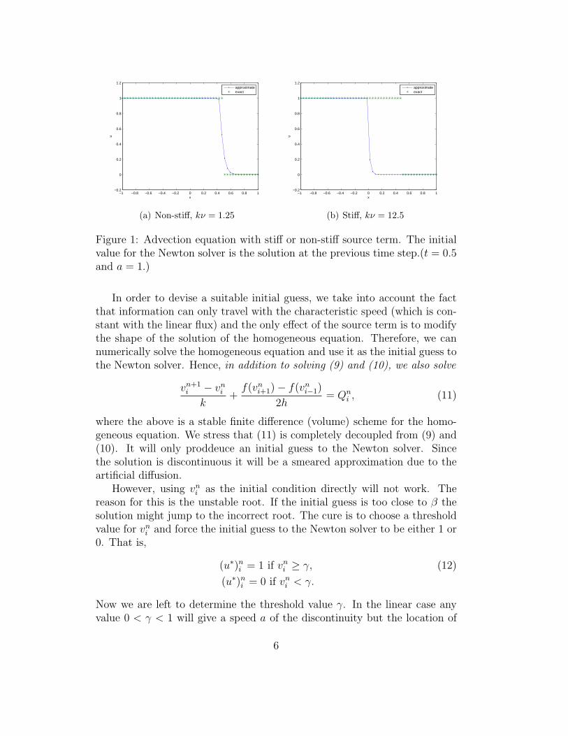
(Note that this is not equivalent to the common fractional step approachsince it is a one-step procedure to update the solution.) At each time step,the non-linear equation (9) is solved with the Newton’s method. Accordingly,we must choose the initial guess, u∗, that will be fed to the Newton solver.The naive guess is of course un

i . This is successful as long as the source isnot stiff, i.e., kν . 1, but in the stiff case the numerical solution remainsstationary. This is shown in Figure 1 for the advection equation (3) att = 0.5 with a = 1. Hence, with this approach we experience exactly thesame difficulties of incorrect propagation speeds in the stiff/under-resolvedcase, as the fractional step methods mentioned in the introduction. Thecorrect solution is a traveling wave at the speed a = 1.

The non-linear source term has 2 stable zeroes, at u = 0 and u = 1 andone unstable root at u = β. It is well-known for the Newton method, that theinitial guess has to be chosen sufficiently close to the desired root. Otherwise,we may converge to the wrong root. The above numerical result forces usto conclude that the initial guess of the Newton solver solely determines thespeed of the computed discontinuity.

5

−1 −0.8 −0.6 −0.4 −0.2 0 0.2 0.4 0.6 0.8 1−0.2

0

0.2

0.4

0.6

0.8

1

1.2

x

u

approximateexact

(a) Non-stiff, kν = 1.25

−1 −0.8 −0.6 −0.4 −0.2 0 0.2 0.4 0.6 0.8 1−0.2

0

0.2

0.4

0.6

0.8

1

1.2

x

u

approximateexact

(b) Stiff, kν = 12.5

Figure 1: Advection equation with stiff or non-stiff source term. The initialvalue for the Newton solver is the solution at the previous time step.(t = 0.5and a = 1.)

In order to devise a suitable initial guess, we take into account the factthat information can only travel with the characteristic speed (which is con-stant with the linear flux) and the only effect of the source term is to modifythe shape of the solution of the homogeneous equation. Therefore, we cannumerically solve the homogeneous equation and use it as the initial guess tothe Newton solver. Hence, in addition to solving (9) and (10), we also solve

vn+1i − vn

i

k+

f(vni+1) − f(vn

i−1)

2h= Qn

i , (11)

where the above is a stable finite difference (volume) scheme for the homo-geneous equation. We stress that (11) is completely decoupled from (9) and(10). It will only proddeuce an initial guess to the Newton solver. Sincethe solution is discontinuous it will be a smeared approximation due to theartificial diffusion.

However, using vni as the initial condition directly will not work. The

reason for this is the unstable root. If the initial guess is too close to β thesolution might jump to the incorrect root. The cure is to choose a thresholdvalue for vn

i and force the initial guess to the Newton solver to be either 1 or0. That is,

(u∗)ni = 1 if vn

i ≥ γ, (12)

(u∗)ni = 0 if vn

i < γ.

Now we are left to determine the threshold value γ. In the linear case anyvalue 0 < γ < 1 will give a speed a of the discontinuity but the location of

6

the discontinuity will differ by O(h). Hence, a naive choice is γ = 0.5 thatresults in the correct propagation speed of the discontinuity (see Figure 2 fornumerical results).

−1 −0.8 −0.6 −0.4 −0.2 0 0.2 0.4 0.6 0.8 1−0.2

0

0.2

0.4

0.6

0.8

1

1.2

x

u

approximateexact

(a) Non-stiff,kν = 1.25

−1 −0.8 −0.6 −0.4 −0.2 0 0.2 0.4 0.6 0.8 1−0.2

0

0.2

0.4

0.6

0.8

1

1.2

x

u

approximateexact

(b) Stiff,kν = 12.5

Figure 2: Advection equation with stiff or non-stiff source term. Initialcondition to the Newton solver is the solution to the advection equationwithout the source term. (γ = 0.5, t = 0.5)

The proposed remedy with an auxiliary solution solves the linear modelproblem irrespective of the choice of γ. The introduction of the auxiliaryproblem and the thresholding of the root is the key step that makes theIMEX scheme work for arbitrarily stiff sources. Trivially, it will also workin the non-stiff case as seen in Figure 2. (A proof of convergence for thenumerical solution, will be given below.)

2.1 Burger’s equation with stiff source term

Consider the non-linear model (6) with initial data (4). The exact solution isa shock with speed 0.5. We apply the same scheme and compute an auxiliarysolution, apply (12) before using it as an initial guess in the Newton solver.We show the solution at t = 4 with β = 0.9 and γ = 0.5 in Figure 3. Wenote that the shock location is given correctly, at x = 2 in both the stiff andnon-stiff case. Again, any choice of the thresholding parameter works in thiscase. In the case of the nonlinear model (6) with initial data (8), we havealready mentioned that the exact solution is a traveling wave moving at thespeed β. In this case, taking the thresholding parameter γ = 0.5 and β = 0.9results in a stable but incorrect solution given in the first part of Figure 4.

In order to resolve the problem, we recall that the role of the source is toforce those values below β to 0 and those above β to 1 in a time scale of 1

ν

7

−5 −4 −3 −2 −1 0 1 2 3 4 5

0

0.2

0.4

0.6

0.8

1

1.2

x

u

approximate solutionauxiliary solution

(a) Non-stiff,kν = 1.51

−5 −4 −3 −2 −1 0 1 2 3 4 5

0

0.2

0.4

0.6

0.8

1

1.2

x

u

approximate solutionauxiliary solution

(b) Stiff,kν = 151

Figure 3: Burgers’ equation with stiff or non-stiff source term. Initial valueto the Newton solver is the solution to Burgers’ equation without the sourceterm. (t = 4, β = 0.9, γ = 0.5)

resulting in a speed of β.We are going to replicate this process. The auxiliary numerical solution

gives a rarefaction wave between 0 and 1. Although, the wave speeds ingeneral differ between the auxiliary solution and the solution with the source,we note that the source term vanishes at u = 0, 1, β. At those presice values,the auxiliary solution and the exact solution have the exact same wave speedsfor all future times. Hence, by choosing the thresholding parameter γ = βfor the initial guess, we precisely obtain the correct speed.

Returning to the above problem with β = 0.9, we note that the wavefront should be at x = 3.6, which is achieved with γ = β. See Figure 4 forthe solution.

2.2 Convergence

So far, we have outlined a numerical scheme for the scalar model equationsand shown its robustness by numerical examples. However, we have not yetformally discussed any convergence properties of the proposed scheme andwe continue by stating two theorems ensuring that the scalar model problemsconverge to a weak solution. We stress that even for the linear flux function,linear theory does not apply due to non-linearity of the source.

It is well known that any standard finite volume scheme with explicitforward Euler time stepping will converge to the entropy solution of a scalarconservation law as the mesh is refined. If one uses a standard finite vol-ume scheme together with explicit forward Euler time stepping for (7), the

8

−5 −4 −3 −2 −1 0 1 2 3 4 5

0

0.2

0.4

0.6

0.8

1

1.2

x

u

approximate solutionauxiliary solution

(a) kν = 151, γ = 0.5

−5 −4 −3 −2 −1 0 1 2 3 4 5

0

0.2

0.4

0.6

0.8

1

1.2

x

u

approximate solutionauxiliary solution

(b) kν = 151, γ = β

Figure 4: Burgers’ equation with stiff source terms. Initial value to theNewton solver is the solution to Burgers’ equation without the source term.(β = 0.9 and t = 4)

approximate solutions will converge to the entropy solution by this standardtheory. Note that in the limit k → 0, the stiffness parameter kν → 0 (forany large but fixed ν) and the standard convergence results apply. However,our IMEX scheme is different from a standard explicit scheme due to theimplicit-explicit nature of the time stepping. None of the standard conver-gence results apply in this case and we will prove convergence to the entropysolution for this IMEX scheme. To the best of our knowledge, this is the firsttime that such a convergence proof has been provided for IMEX schemes fornon-linear conservation laws.

We start with the linear problem. Consider the generic linear advectionequation with a non-linear source,

ut + aux = S(u), (13)

where we have considered a constant velocity a for simplicity. Using standardnotation for finite differences given by

D+x (bi) =

1

h(bi+1 − bi), D−

x (bi) =1

h(bi − bi−1)

D0x(bi) =

1

2h(D+

x (bi) + D−x (bi))

we rewrite the first-order IMEX scheme for (13) as,

D−t (un+1

i ) + aD−x (un

i ) = S(un+1i ). (14)

This scheme is the upwind scheme and is the specific form of the Roe’s schemefor the linear equation. Furthermore define the following piecewise constant

9

function,

u∆ =∑

j,n

χj,nunj ,

where χj,n is the Characteristic function of the cell [xi−1/2, xi+1/2)× [tn, tn+1)Then, we have the following convergence theorem for (14).

Theorem 2.1 Consider the advection equation (13) with a smooth source Ssuch that there exists a large constant C and a positive constant c1 such that

S(w) ≤ −c1w2k−1, if w ≥ C, (15)

for k ∈ {1, 2, · · · , }. Let uni be defined by the scheme (14) and the function u∆

be defined as above. Furthermore, we assume the following CFL condition,

ak

h≤

1

2, (16)

and assume that the initial data u0 ∈ H1(R). Then, the approximate solu-tions satisfy the following estimates,

h∑

i

(un+1i )2 ≤ h(

∑

i

(uni )2 + C), (17)

where C is a positive constant and

h∑

j

(un+1i − un+1

i−1 )2 ≤ Ch(∑

i

(u0i − u0

i−1)2). (18)

Furthermore, we have that u∆ → u a.e where u is the unique weak solutionof (13).

We omit the proof of the estimates (17) and (18), since it is similar to theproof of the estimates in the next theorem. The above BV type estimate(18) is enough to obtain strong convergence of the approximate solutions.We move on and consider the non-linear scalar conservation law

ut + (f(u))x = S(u). (19)

The IMEX scheme (9) can be rewritten as

D−t (un+1

i ) + D−x (Gn

i ) = S(un+1i ), (20)

where the numerical flux Gni = G(un

i , uni+1) refers to any consistent, monotone

two point flux for the flux function f . We need some general results about

10

numerical schemes for scalar conservation laws. First, following [11], wedenote Qn

i as the numerical viscosity associated with the flux G given by

Qni =

f(uni ) + f(un

i+1) − 2G(uni , u

ni+1)

uni+1 − un

i

, if uni+1 6= un

i ,

= 0, otherwise.

Next, we take the entropy function U(u) = u2 and the associated entropyflux η(u) =

∫ s

0u(s)f ′(s)ds. Following [12], the entropy potential Ψ is given

by Ψ(u) = uf(u)− η(u). By [12], the unique entropy conservative numericalflux corresponding to the above entropy functions is given by

Gni =

Ψ(uni+1) − Ψ(un

i )

uni+1 − un

i

, if uni+1 6= un

i ,

= 0, otherwise.

In addition to the consistency and monotonicity of G, we assume that for alln, j,

Qni − Qn

i ≥ α,

where α is a positive constant. Thus, we choose a numerical flux, which hasgreater viscosity than the entropy conservative flux. The numerical viscosityassociated with Gn

i is denoted by Qni . A number of choices of numerical

fluxes satisfy the above criteria. They include the Godunov flux, the EnquistOsher flux and the Roe flux with an entropy fix. Then, we have the followingconvergence theorem for (20).

Theorem 2.2 Consider the non-linear scalar conservation law (19) with asmooth flux f such that f is genuinely non-linear, i.e., it does not containany piecewise linear segments and a smooth source S satisfying (15). Letun

i be defined by the scheme (20) and the function u∆ be defined as above.Furthermore, we assume the following CFL condition,

maxn,i

(|f ′(un

i )|2

(Qni − Qn

i )

)k

h≤ 1/4, (21)

where Qni , Qn

i are defined above. We also assume that the initial data u0 ∈L∞(R) ∩ L2(R). We have the following entropy (energy) estimate ,

h∑

j

(un+1i )2 ≤ h(

∑

j

(uni )2 + C), (22)

11

where C is a positive constant. Furthermore, we have the “weak” BV esti-mate,

h∑

n,i

|uni − un

i−1|2 ≤ C (23)

In addition to the above, if we assume that

maxn,j

|unj | ≤ C

then we have that u∆ → u a.e as h, k → 0 and u is a weak solution of (19).

Proof Note that the hypothesis (15) on the source S are trivially satisfiedby the source in (7) and the above convergence result holds for this specialcase. We need the following discrete chain rule,

D±x (a2

i ) = 2aiD±x (ai) ± h(D±

x ai)2.

We start by multiplying both sides of (20) by 2un+1i and apply the above

chain rule and adding and subtracting terms to get,

D−t ((un+1

i )2) + k(D−t (un+1

i ))2 + 2kD−t (un+1

i )D−x (F n

i ) + (24)

2uni D−

x (F ni ) = un+1

i S(un+1i ).

By standard Cauchy inequality, we have that,

−2kD−t (un+1

i )D−x (Gn

i ) ≤ k(D−t (un+1

i ))2 + k(D−x (Gn

i ))2.

Next, denote

Hni =

G(uni , u

ni+1) − f(un

i )

uni+1 − un

i

.

By consistency of the numerical flux G, we have

(D−x Gn

i )2 ≤ 2k(Hni )2(D−

x uni )2 + 2k(Hn

i−1)2(D+

x uni )2.

We need to control the term 2uni D−

x (Gni ). For this, we use the entropy dis-

sipation estimate from [12](Theorem 5.2) for this special case. Define thenumerical entropy flux as,

Hn

i =1

2((un

i + uni+1)G

ni ) −

1

2(Ψ(un

i ) + Ψ(uni+1)).

Then we have that

2uni D−

x (Gni ) = D−

x Gn

i + h((Qni − Qn

i )(D−x un

i )2) + h((Qni−1 − Qn

i−1)(D+x un

i )2).

12

Using both the above inequalities and summation by parts in space (ignoringthe boundary terms by taking data with compact support), we rewrite (24)as,

∑

i

D−t ((un+1

i )2) ≤− (h

2(Qn

i − Qni ) − 2kHn

i )∑

i

(D−x (un

i ))2

− (h

2(Qn

i−1 − Qni−1) − 2kHn

i−1)∑

i

(D+x (un

i ))2 (25)

− (h

2(Qn

i − Qni )

∑

i

(D−x (un

i ))2)

− (h

2(Qn

i−1 − Qni−1)

∑

i

(D+x (un

i ))2) +∑

i

un+1i S(un+1

i ).

Using the definition of Hni and the CFL condition (21), we get that,

∑

i

D−t ((un+1

i )2) ≤∑

i

un+1i S(un+1

i ). (26)

Next from the hypothesis (15) on the source S, there exists a large constantC and a positive constant c1 (independent of mesh parameters) such that

wS(w) ≤ −c1w2k, if w ≥ C.

Hence, we can divide the set of mesh points i into two sets I1 and I2 suchthat

I1 = {i ∈ Z : un+1i ≤ C},

I2 = {i ∈ Z : un+1i > C}.

Using this division and rewriting (26) we get,

h∑

i

D−t ((un+1

i )2) ≤ h(∑

i∈I1

un+1i S(un+1

i ) +∑

i∈I2

un+1i S(un+1

i ))

≤ C − c1h∑

i∈I2

(un+1i )2k

≤ C,

where we denote different mesh independent positive constants by C. Henceand using the CFL condition, we get the bound

h∑

(un+1i )2 ≤ h(

∑(un

i )2 + C),

13

which proves the energy bound (22). Furthermore, by using (22), the factthat for all n, i, (Qn

i − Qni ) ≥ α and summing over all n in (25), we get that

h∑

n,i

(D−x un

i )2 ≤ C

Thus, proving the “weak” BV estimate (23).Now, by using (23) and the assumption that the approximate solutions u∆

are bounded in L∞, we can appeal to the theory of compensated compactnessfor scalar conservation laws (for details refer to [13]) in order to get thatu∆ → u (upto a subsequence) as h → 0. Due to the strong convergence, wecan pass to the limit in both the non-linear flux and source terms in (19) andconclude that u is a weak solution of (19)

Note that the proof of theorem 2.2 requires genuine non-linearity on theflux function f and doesn’t apply directly to the linear advection equation.Hence theorem 2.1 is not a special case of theorem 2.2.

Remark For convergence proof in the non-linear case, we need to assumethat the approximate solutions are bounded in L∞. This is technical innature as we are unable to prove that such a bound holds. In addition tothis, the bound is reasonable at least in the stiff case, i.e., ν >> 1 as theroots of the equation (20) will be close to 0 and 1 in this case.

Remark The CFL condition (21) is very stringent in the proof of conver-gence. It essentially amounts to choosing k small enough. Again, we stressthat this is technical and we were able to get good numerical results byrunning at the standard convective CFL number given by

maxn,i

|f ′(uni )|

k

h≤

1

2,

which is also consistent with CFL condition (16) for the linear problem.

2.3 Summary of scheme

Next, we summarize the proposed scheme for the scalar model problems.

1. Compute Rni = − k

2h(fn

i+1 − fni−1) + kQn

i .

2. Compute the auxiliary solutionvn+1

i−vn

i

k+

f(vni+1

)−f(vni−1

)

2h= (Qv)

ni .

14

3. Compute the initial guess to the Newton solver:

(u∗)ni = 1 if vn

i ≥ β, (27)

(u∗)ni = 0 if vn

i < β. (28)

4. Solve the equation un+1 −kν(1−un+1i )(un+1

i −β)un+1i = Rn

i with New-ton’s method.

The arguments and the listing of the final algorithm have all been done forthe first-order IMEX scheme but it is trivial to generalize it to a high-orderARK scheme, where each stage is treated according to our solution scheme.We stress that this time-integration algorithm is completely independent ofthe choice of spatial approximation. Furthermore, we emphasize that theinitial guess to the Newton solver only specifies the location of the wave.It does not affect the accuracy in any other aspect. Many different choicesof initial guesses would lead to the same approximate solution of the stiffequation, as long as the discontinuity is at the correct location.

The auxiliary function and the construction of the initial guess to theNewton solver can be viewed as a subgrid scale model that recovers theinformation that is lost by taking larger time steps than the chemical timescale. Indeed, it comes at a cost. We need to carry one extra solution field,which doubles the computational work. However, this is a small price topay to be able to march at the convective CFL. We also note that there isa considerable extra work and memory required in the methods proposed in[2, 7]. In [7] they do not even consider the nonlinear model problem withthe rarefaction wave, which is considerably more difficult to solve than theshock solutions. To our knowledge the scalar model problem with rarefactionwave initial data has never been successfully computed previously.

2.4 Further numerical tests

To demonstrate that the technique is general and applicable to a wider rangeof problems, we change the flux to f(u) = u4

4and use the initial data (4). The

Rankine-Hugoniot condition suggests a shock speed of 0.25 and in Figure 5we show the solution at T = 4 and β = 0.4. We should find the shockat x = 1, regardless of the value of β, and indeed that is the case. As forBurgers’ equation, the choice of β is not crucial to obtain the correct shocklocation. Hence, we continue with the initial data (8). By the results of[14], we should see a traveling wave at the speed f ′(β) = β3. We chooseβ = 0.7937 such that the speed becomes 0.5. In this case the front should beat x = 2 at t = 4. This is clearly seen in Figure 5.

15

−5 −4 −3 −2 −1 0 1 2 3 4 5

0

0.2

0.4

0.6

0.8

1

x

u

approximate solutionauxiliary solution

(a) kν = 651, β = 0.4

−5 −4 −3 −2 −1 0 1 2 3 4 5

0

0.2

0.4

0.6

0.8

1

x

u

approximate solutionauxiliary solution

(b) kν = 651, β = 0.7937

Figure 5: Burgers’ equation with stiff source terms. Initial condition to theNewton solver is the solution to Burgers’ equation without the source term.n = 50, t = 4

Next, we reconsider Burgers’ equation. This time with initial data

u(x, 0) = 0.5sin(2πx

L) + 0.5, L = 10. (29)

and subject to periodic boundary conditions. The equation will drive thesolution towards 0 or 1. The speed of this process is 1

ν. The solution becomes

essentially piecewise constant and the discontinuities travel with the shockspeed (or β depending on the direction of the jump).

Next, consider the proposed solution method. The auxiliary solution de-termines the locations of the discontinuities. It will follow the characteristicu(x, t) = β until the auxiliary solution forms a shock. Then the jump condi-tion at the shock determines the speed shock. Hence, the true solution formsa shock front after a time t ∼ 1

ν, while the scheme will form a shock only

when the homogeneous Burgers’ equation has formed a shock after the timeTshock. After that both the true solution and the numerical solution move thediscontinuity at the shock speed. However, the error of the initial behaviorgives a constant error in the numerical solution. (It will not disappear withgrid refinement.) If the problem is nonstiff the error will be small and if it isstiff it is large. These effects can be observed in the computations.

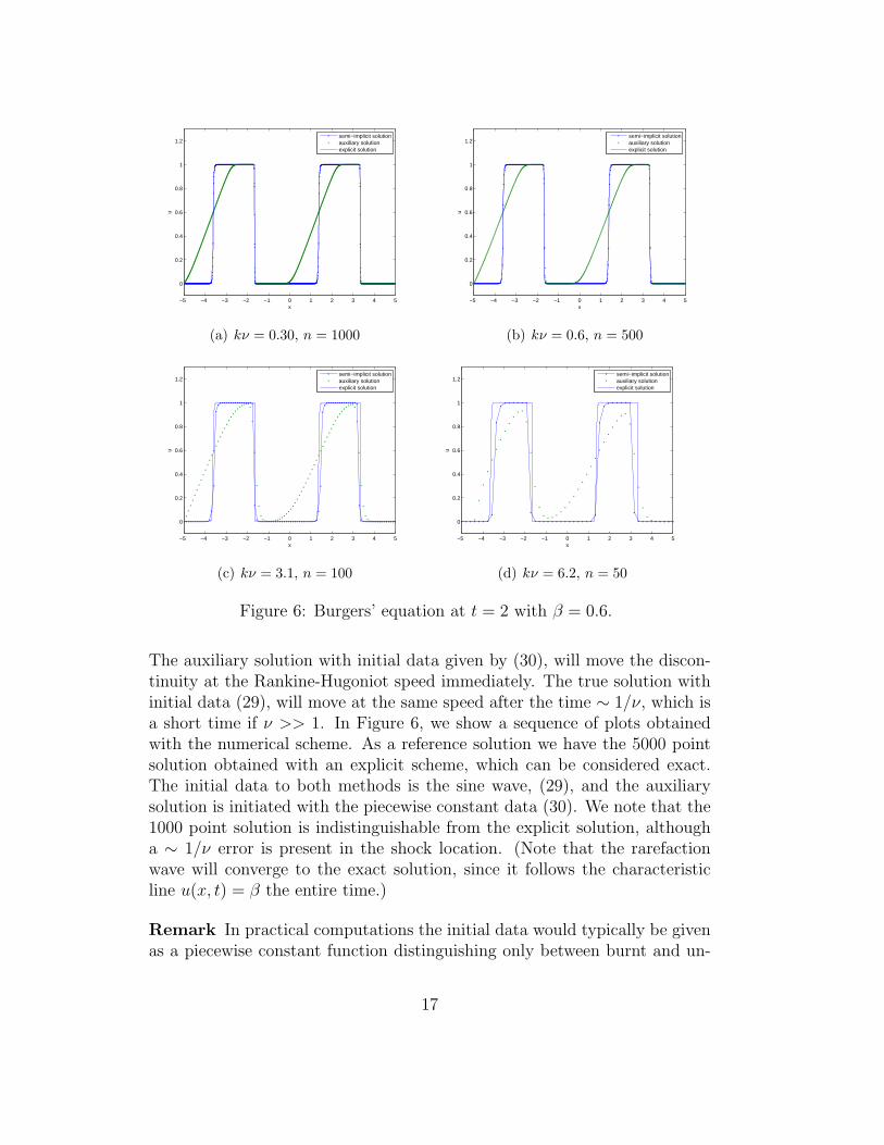
Since the aim is compute solutions in the stiff case, we make the followingobservation. We change the initial data (29), for the auxiliary solution to

u∗(x, 0) = 1 if u(x, 0) > β, (30)

u∗(x, 0) = 0 if u(x, 0) < β.

16

−5 −4 −3 −2 −1 0 1 2 3 4 5

0

0.2

0.4

0.6

0.8

1

1.2

x

u

semi−implicit solutionauxiliary solutionexplicit solution

(a) kν = 0.30, n = 1000

−5 −4 −3 −2 −1 0 1 2 3 4 5

0

0.2

0.4

0.6

0.8

1

1.2

x

u

semi−implicit solutionauxiliary solutionexplicit solution

(b) kν = 0.6, n = 500

−5 −4 −3 −2 −1 0 1 2 3 4 5

0

0.2

0.4

0.6

0.8

1

1.2

x

u

semi−implicit solutionauxiliary solutionexplicit solution

(c) kν = 3.1, n = 100

−5 −4 −3 −2 −1 0 1 2 3 4 5

0

0.2

0.4

0.6

0.8

1

1.2

x

u

semi−implicit solutionauxiliary solutionexplicit solution

(d) kν = 6.2, n = 50

Figure 6: Burgers’ equation at t = 2 with β = 0.6.

The auxiliary solution with initial data given by (30), will move the discon-tinuity at the Rankine-Hugoniot speed immediately. The true solution withinitial data (29), will move at the same speed after the time ∼ 1/ν, which isa short time if ν >> 1. In Figure 6, we show a sequence of plots obtainedwith the numerical scheme. As a reference solution we have the 5000 pointsolution obtained with an explicit scheme, which can be considered exact.The initial data to both methods is the sine wave, (29), and the auxiliarysolution is initiated with the piecewise constant data (30). We note that the1000 point solution is indistinguishable from the explicit solution, althougha ∼ 1/ν error is present in the shock location. (Note that the rarefactionwave will converge to the exact solution, since it follows the characteristicline u(x, t) = β the entire time.)

Remark In practical computations the initial data would typically be givenas a piecewise constant function distinguishing only between burnt and un-

17

burnt state. In that case the implicit-explicit scheme computes the correctsolution without any errors due to initial transients.

3 Part II: The reactive Euler equations

The previous model problems, although challenging, have no physical mean-ing and we now shift our focus to the reactive Euler equations. We willrestrict ourselves to one space dimension, since the generalization to multi-ple space dimensions is straightforward.

We begin by writing the first-order IMEX scheme. We specify the fol-lowing notation for the first three unknowns and fluxes in the reactive Eulerequations,

u = {ρ, ρu,E}, F = {ρu, ρu2 + p, (E + p)u},

Also let (Qu)ni , (Qz)

ni be artificial dissipation terms correspoding to the un-

known vector u and the unknown ρz respectively. The exact structure of thedissipation terms will be specified later. Then, the first-order IMEX schemefor the reactive Euler equations takes the form,

un+1i − un

i

k+

F ni+1 − F n

i−1

h= (Qu)

ni

(ρz)n+1i = Rn

i − kK(T ∗)(ρz)n+1i (31)

Rni = (ρz)n

i − k(ρz)n

i+1 − (ρz)ni−1

h+ (Qz)

ni .

From the above scheme, it is clear that un+1i can be obtained explicitly and

it determines the flow variables at the next time step. Furthermore, we useun and zn to choose T ∗ = T n. Given T ∗, (ρz)n+1

k can now be solved directlysince it is a linear equation. We notice an important difference from the scalarexamples where the source term depends solely on the solution variable itself,whereas for the Euler equations ρz is driven by the Euler solution in eachtimestep.

Next, we will discuss the choice of the artificial dissipation operator. Thisis the crucial step in obtaining correct propagation speeds on under-resolvedmeshes. Assuming that we have a stable scheme for the non-reactive Eulerequations, Qu can be determined directly keeping in mind that p (or equiv-alently T ) is now a function of z as well. We use the Roe scheme for ourcomputations. To determine the dissipation required for the ρz equation in(31), we analyze stability of the linearized equation with frozen coefficients.The linearized Euler equations can be symmetrized as proposed in [15] and

18

the resulting difference scheme takes the form,

wn+1i − wn

i

k+ ADwi = 0 (32)

(ρz)n+1i = Rn

i − kK(T ∗)(ρz)n+1i (33)

Rni = (ρz)n

i − kui

(ρz)ni+1 − (ρz)n

i−1

h+ (Qz)

ni .

where A is a constant symmetric matrix and ui the ”frozen” value of thevelocity. The tilde sign highlights that the independent variables are thelinearly perturbed variables. w is the vector of the first three perturbedvariables associated with the Euler equations. D signifies the operator thatapproximates the space derivative. We assume that it contains sufficient dis-sipation to stabilize the Euler part. In any case, the last equation decouplesin the linear analysis and is driven only by the frozen coefficient ui. Hence, wesimply have to analyze the following model to determine the linear stabilityproperties of the full reactive Euler equations,

ut + aux = −Ku

where K is a large constant. Its discretization becomes

vn+1j = vn

j −ak

2h(vn

j+1 − vj−1) − kKvn+1j +

kǫ

h(vj+1 − 2vj + vj−1).

First, we will consider the case K = 0. We use von Neumann analysis andmake the ansatz vn

j = vn(ξ)eijξ −π ≤ ξ ≤ π. Denote λ = akh

. Then,

vn+1 = (1 − λisin(ξ))vn +kǫ

h(−2 + 2cos(ξ))vn.

Posing the scheme as vn+1 = g(ξ)vn, the stability requirement is |g(ξ)| ≤ 1.

Hence, we require ǫ = |a|2

, which gives the well-known upwind scheme (orRoe scheme).

Next, consider the case K >> 1 and ǫ = 0 using von Neumann analysis.

vn+1 = (1 − λisin(ξ))vn + kKvn+1

vn+1 =1 − λisin(ξ)

1 + kKvn

In this case we see that the scheme is stable without artificial dissipation forkK > 1. However, as kK approaches 1 we need to add the standard upwinddissipation in the ρz equation. We do so by introducing the scaling function

W (kK) =

{1 − kK, if kK < 1,

0, if kK ≥ 1,

19

and adding the following upwind dissipation,

(Qz)ni = W (kK)

|uni |

2h((ρz)n

i+1 − 2(ρz)ni + (ρz)n

i−1),

Thus completing the scheme (31). This analysis reflects the fact that thesource term in the mass fraction equation of the reactive Euler equationsis dissipative and dissipation is proportional to the stiffness. Hence, forlarge time steps, we do not have to add numerical diffusion to stabilize thecomputations and this means that the shocks remain sharp and move withthe right speed of propagation.

Before we move on to the computations we make a final remark. The de-pendence of z in the Euler dissipation (Qu) will actually decrease the amountof dissipation for the Euler part of the equations as well. We also stress thatthe effective amount of dissipation for the Roe scheme is dependent on theratio k/h. If we take that ratio smaller, the effective dissipation will increase,which will be evident in the computations below.

3.1 Computations

To test the scheme, we use the same benchmark case as in [2, 7]. We useA = 164180, TA = 25, q0 = 25, γ = 1.4. The initial conditions are two states.The burnt state is: ρb = 1.6812, ub = 2.8867, pb = 21.5672, zb = 0. Theunburnt state is: ρub = 1, uub = 0, pub = 1, zub = 1. The solution is a CJwave traveling at a speed s = 7.1247. We initiate with the discontinuity atx = 0 and compute to t = 1. n denotes the number of grid points used todiscretize the x-axis.

Stiff case: The solution for n = 100 and n = 300 is shown in Figure7. No diffusion is added to the ρz equation. We conclude that the schemecaptures the correct solution. (We mark the shock location but that curvedoes not represent the true solution, which has an overshoot.)

Case with less stiffness: In Figure 8, we also show the solution withn = 1000, which is less stiff due to higher resolution.

Smaller CFL: The first cases were obtained with the same CFL ratiok/h. If we divide the CFL number by 2, the shape of the solution will change,since the effective dissipation will increase as discussed above. This is shownin Figure 8, where the solution becomes more smeared.

Diffusion in the ρz equation: To show the effect of diffusion in theρz equation, we have computed two examples. The first has a undividedsecond difference as diffusion term and the second has a larger diffusionwhere the undivided difference has been multiplied by 1/h. The latter isa standard upwind shock capturing scaling and it can be seen in Figure 9

20

−5 0 5 10 15 20 250

5

10

15

20

25

x

p

approximate solutionshock location

(a) n = 100,kK(Tb) = 410

−5 0 5 10 15 20 250

5

10

15

20

25

x

p

approximate solutionshock location

(b) n = 300,kK(Tb) = 133

Figure 7: Pressure solution for detonation shock wave at t = 1.

−5 0 5 10 15 20 250

5

10

15

20

25

x

p

approximate solutionshock location

(a) n = 300,kK(Tb) = 66

−5 0 5 10 15 20 250

5

10

15

20

25

30

x

p

approximate solutionshock location

(b) n = 1000,kK(Tb) = 40

Figure 8: Pressure solution for detonation shock wave at t = 1 with 2nd-orderscheme, a thousand grid pointss and a small time step.

that an erroneous shock appear. The behavior is very similar to what hasbeen reported in [2, 7, 8]. However, we note that the case with the smallerdiffusion term in Figure 9, the solution is correct and hardly different fromthe non-diffusive case in Figure 7.

Non-stiff case: Finally, we demonstrate that the method works in thenon-stiff limit, we compute a 10000 point solution shown in Figure 10.

Remark We have shown that we do not need diffusion in the ρz equation,but the scheme does not fail if we add a small amount of diffusion and smearthe z-profile a little bit. However, if we add lots of diffusion we will see thesame erroneous behavior as has been reported previously in [2, 7, 8]. Forsmall time steps, we need diffusion in the z equation according to the von

21

−5 0 5 10 15 20 250

5

10

15

20

25

x

p

approximate solutionshock location

(a) n = 300,kK(Tb) = 133, small diffusion

−5 0 5 10 15 20 250

5

10

15

20

25

x

p

approximate solutionshock location

(b) n = 300,kK(Tb) = 133, large diffusion

Figure 9: Pressure solution for detonation shock wave at t = 1 with 2nd-orderscheme, 300 grid points and differently sized artificial diffusion.

Neumann analysis.

4 Conclusions

In this article, we have addressed two different types of equations with stiffsource terms. The main goal was to devise a scheme that uses a time stepgoverned by the flow and not the stiff source term. We choose an IMEXtime integration scheme due to its flexibility. It allows us to treat the sourceimplicitly and in addition, it also allows the user to treat other terms likediffusion and heat conduction implicitly. Furthermore, it is independent ofthe spatial discretization which makes a generalization to multiple dimensionsor higher-order schemes straightforward. The IMEX scheme is not designedexclusively for the stiff case but handles the non-stiff case as well. Finally,the IMEX scheme can be viewed as a single stage in a high-order AdditiveRunge-Kutta scheme (see [9, 10]) allowing for high-order approximations ofthe temporal derivative.

Although based on the same IMEX scheme, the scalar model and thereactive Euler equations were analyzed separately as the dynamics differ inboth cases.

In Part I, the scalar model problem was studied. The key observationwas that the initial guess to the Newton solver defined the location of thewave front entirely. Hence, an auxiliary numerical solution was necessary togenerate the initial guess for each time step. For this scheme, we have provedthat it converges to a weak solution. For a linear flux this can be furtherstrengthened and we show convergence to the correct weak solution. For

22

−5 0 5 10 15 20 250

5

10

15

20

25

30

35

xp

approximate solutionshock location

(a) n = 10000,kK(Tb) = 3.94

Figure 10: Pressure solution for detonation shock wave at t = 1 with 2nd-order scheme with 10000 grid points.

the non-linear flux, we outline arguments showing that the right solution isobtained. Numerous numerical computations support the theoretical results.In particular we point at the successful computation with rarefaction initialdata. To our knowledge, this is the first time that it has been done.

In Part II, we designed schemes for the reactive Euler equations. Since theflow equations determine the wave front, no auxiliary solution is necessary.The only precaution that has to be taken, is that the amount of artificialdiffusion added to the reaction equation must not be too large. We showedwith a linear analysis that no numerical diffusion is needed as long as theequation is stiff. As the solution is more resolved, i.e., the problem becomesnon-stiff, we have to add numerical diffusion and the problem behaves as astandard hyperbolic equation. We have confirmed these findings with nu-merical computations and also demonstrated that the scheme works equallywell in the non-stiff case.

Hence, this approach is cheaper, less memory consuming and simpler tocode than previously proposed remedies. It is much more flexible to adoptthis technique as it only requires a change of the temporal discretizationscheme.

References

[1] R.J. LeVeque. Numerical Methods for Conservation Laws. BirkhauserVerlag, Basel, 1990.

[2] C. Helzel, R. J. LeVeque, and G. Warnecke. A modified fractional step

23

method for the accurate approximation of detonation waves. SIAMJ.Sci.Comput., pages 1489–1510, 2000.

[3] P. Colella, A. Majda, and V. Roytburd. Theoretical and numericalstructure for reacting shock waves. SIAM J. Sci. Stat. Comput., 7:1059–1080, Oct. 1986.

[4] B. Sjogreen and B. Engquist. Numerical approximation of hyperbolicconservation laws with stiff source terms. In in Hyperbolic Problems.Theory, Numerical methods and applications, Uppsala, Sweden, Vol II,pages 848–860, 1990.

[5] A.C. Berkenbosch, E.F. Kaasschieter, and R. Klein. Detonation cap-turing for stiff combustion chemistry. Combust. Theory. Model, pages313–348, 1998.

[6] A.C. Berkenbosch. Capturing detonation waves for reactive Euler equa-tions. PhD thesis, T.U. Eindhoven, The Netherlands, 1995.

[7] L. Tosatto and L. Vigevano. Numerical solution of under-resolved det-onations. accepted manuscript, JCP, 2007.

[8] R.J. LeVeque and H.C. Yee. A study of numerical methods for hy-perbolic conservation laws with stiff source terms. J. Comput. Phys.,86:187–210, 1990.

[9] C.A. Kennedy and M. H. Carpenter. Additive runge-kutta schemes forconvection-diffusion-reactio equations. Applied Numerical Mathematics,44:139–181, 2003.

[10] M. H. Carpenter, C.A. Kennedy, H. Bijl, S.A. Viken, and V. N.Vatsa. Fourth-order runge-kutta schemes for fluid mechanics applica-tions. Journal of Scientific Computing, 25:157–194, 2005.

[11] E. Godlewski and P. A. Raviart. Hyperbolic systems of conservationlaws. Mathematiques et Applications, Ellipses, Paris, 1991.

[12] E. Tadmor. The numerical viscosity of entropy stable schemes for sys-tems of conservation laws, i. Math. Comp., 49:91–103, 1987.

[13] Y. Lu. Hyperbolic conservation laws and the compensated compactnessmethod. Surveys in Pure and Applied Mathematics, Chapman and Hall,CRC, Boca Raton, Fl., 2003.

24

[14] H. Fan, S. Jin, and Z.H. Teng. Zero reaction limits for hyperbolic con-servation laws with source terms. J. Diff. Eqns., 168(2):270–294, 2000.

[15] T.H. Pulliam and D.S. Chaussee. A diagonal form of an implicitapproximate-factorization algorithm. J. Comput. Phys., 39:347–363,1981.

25