Modeling bolts in LS-DYNA© using explicit and implicit time ...

15th International LS-DYNA® Users Conference Table of Contents

June 10-12, 2018 1

Modeling bolts in LS-DYNA© using

explicit and implicit time integration

Nils Karajan1, Alexander Gromer1, Thomas Borrvall2, Kishore Pydimarry3 1DYNAmore Corporation, 565 Metro Place South, Suite 300, Dublin, Ohio, 43017, USA 2DYNAmore Nordic, Brigadgatan 5, 58758 Linköping, Sweden 3Honda R&D Americas, Inc., 21001 State Route 739, Raymond, Ohio 43067, USA

Abstract

When setting up models for analysis using the explicit solver in LS-DYNA, the method of how to model bolted

connections is usually well known. However, when this model or even just certain substructures of the model

are used for load cases to be solved using the implicit solver in LS-DYNA, problems might arise that you might

have not been aware of before. Typical automotive load cases for LS-DYNA implicit involve door sag, seat pull,

misuse and other problems that are running over a long time span.

The goal of this contribution is to review the different modeling techniques for friction grip bolts in view

of their respective spatial discretization, their required contact definitions, their pre-tension application and

their load carrying behavior. Moreover, typical problems that arise during explicit and implicit time integration

are discussed and solutions to these potential problems are provided. While these potential problems are often

overseen in explicit, they become very apparent in implicit simulations when the user runs into convergence

problems. This may especially be the case during the pre-tensioning phase of the bolt, when the friction grip

connection starts to slip or ultimately fail.

Finally, a summary is given pointing out the current limitations as well as best practice approaches for

four different types of modeling approaches for friction grip bolts, which can be downloaded from

www.dynaexamples.com/connections/bolts.

Motivation

During the past three decades, LS-DYNA has been established as the standard solver for explicit analysis at

many automotive, aerospace and defense companies worldwide. The predominant application always was and

still is crash worthiness and other high-dynamic impact investigations. Hence, the typical LS-DYNA user has

finite-element models that have been designed and built to run using the explicit solver of LS-DYNA.

Over time, the implicit capabilities of LS-DYNA have matured to a powerful simulation environment,

which is well suited to solve problems with even several million elements as well as quasi-static or low-

dynamic load cases with longer time spans. The benefit of switching to implicit are application specific and

range from shorter simulation times in the case of very small element sizes to smoother response curves.

Following this, more and more users want to take their “explicit” models and simply use them with the

implicit solver of LS-DYNA. This so-called one model strategy is possible to achieve but not all features of the

explicit solver are available for implicit usage. To have a model working in explicit and implicit, certain model-

ing guidelines have to be followed. Sometimes, a material model or a specific element type is not yet available

but ongoing code enhancements should narrow that gap even further in the future. However, the prevalent mate-

rial models used in explicit are well supported by the implicit solver and even tricky contact situations can be

mastered by applying the mortar contact option.

The goal of this contribution is to present four modeling strategies for friction grip connections with

bolts and to point out possible pitfalls during the modeling process of such connections.

www.dynaexamples.com/connections/bolts


June 10-12, 2018 2

Friction Grip Bolts

Definitions and load bearing mechanism

This contribution is focused on bolted connections as shown in Figure 1a) where a threaded fastener with a

head, a shank and an external male thread is pre-tensioned by a nut to join two or more sheets or blocks of ma-

terial. Washers may be included to distribute pre-tensioning loads more evenly or to prevent the bolt to become

loose but are neglected in this work for the sake of simplicity.

a) b) c)

Fig. 1: a) Illustration of a bolt with its head, shank and thread as well as a washer disc to distribute stresses

and a nut to pre-tension the connection b) load bearing behavior during service loads by friction and c)

load bearing behavior for loading states beyond service load leading to bolt hole bearing (all pictures

taken from Wikipedia).

The bolted connections under investigation are based on sufficient friction grip such that all service loads are

carried by static friction between the connected sheets. Thus, applied service loads will not cause any relative

motion or slip in the connection, cf. Figure 1b). To achieve a good grip, the bolts are typically pre-tensioned in

the range of 75% or 90% of the proof load of the high strength bolt material for reusable or permanent connec-

tions, respectively. If the so-called friction grip bolt connection is loaded beyond working conditions, i. e. dur-

ing a crash loading, the static friction may be overcome as is shown in Figure 1c) leading to a slip between the

sheets such that the hole bearing behavior will govern the shear load of the bolt and thus, the ultimate load of

the connection.

The failure of bolted connections at ultimate load can be dominated either by plate tear-out failure or by

bolt shear fracture. As the implicit investigation of typical load cases like misuse or door sag do not involve

failure of the bolted connections, the detailed failure modes are not investigated in this contribution. Instead, the

interested reader is referred to the works of [1-5].

Modeling techniques for pre-tensioned bolts

Meanwhile there are many different possibilities available how bolted connections can be modeled in LS-

DYNA. The technique of choice depends on the loading stages that need to be captured, i.e. is it sufficient to

capture loads in the friction grip regime or will slip or ultimate load be of interest, too. A good overview of

modeling techniques can be found in Sonnenschein [1]. For the sake of completeness, we will briefly review the

modeling possibilities for an explicit simulation and then highlight the necessary changes for successful implicit

simulations. Benefits and merits of the respective modeling technique as well as possible pitfalls will also be

summarized.

In general, there are two main modeling groups for pre-tensioned bolts. These can be distinguished by

the discretization of the shank, which can be carried out using either beam or solid elements. If it is done using a

beam element, it needs to be a “spot weld beam” (ELTYPE=9 in *SECTION_BEAM), which has to be used to-


June 10-12, 2018 3

gether with *MAT_SPOTWELD to be able to use *INITIAL_AXIAL_FORCE_BEAM to apply a pre-tension in

the bolt. In cases were the shank is modeled with solid elements, a pre-stress is introduced via

*INITIAL_STRESS_SECTION.

These two groups are further subdivided depending on the discretization of the head and the nut, which

can be done using beam spiders, shell elements or solid elements. Keep in mind that shell elements have no ro-

tational degrees of freedom around the shell normal. Thus, the bolt is not able to carry torsion loads, if the shank

is discretized with a beam element and the nut as well as the bolt head is modeled with shell elements. Similar

holds for a shank made of beam-elements that is connected to a head and a nut discretized by solid elements.

Different combinations of these possibilities allow for several modeling techniques. The techniques

shown in Fig. 2 are frequently used but variants of those four types can of course also be used.

Type a) type b) type c) type d)

Fig. 2: Illustration of the presented bolt modeling techniques type a) to d).

Bolt Modeling Techniques in Detail

Type a) Beam element for shank and beam-spider mesh connection to connected parts

General remarks

The shank is represented by one beam element while the head and nut (including washers) are represented by

circular beam spider meshes that connect to the perimeter nodes of the bolt holes in the connected sheet metals

or blocks. Herein, the beam spider mesh can represent either deformable beam elements or simply a nodal rigid

body. In the case of two connected parts, there is typically no need to define a contact interface between the bolt

shank and the bolt holes as well as the bolt head or nut and the outside clamped parts. To capture the contact

between the connected materials, a *CONTACT_AUTOMATIC_SINGLE_SURFACE definition is sufficient. If a

third sheet or block is present in the connection, please refer to the type b) connection on how to model its con-

tact with the shank.

Explicit vs. implicit time integration

During implicit runs, it is generally recommended to use the _MORTAR option in the contact definition, to

achieve a better convergence behavior. Thus, the switch to implicit simulations is straightforward and it is usu-

ally sufficient to add the _MORTAR option to the global contact definition of choice. This works fine in the case

of two connected parts. For more connected parts where a slipping motion of the middle sheet might occur,

please refer to connection type b).

Merits and drawbacks

This is the simplest and fastest way of modeling friction grip bolts to connect two parts consisting of shell or

solid elements. A drawback of this modeling technique lies in its simplicity. Herein, a slipping motion can only

be captured between the connected parts but never between the nut or the head and the connected parts, as the

beam-spider mesh is sharing nodes with shell or solid elements of the connected parts. Following this, any slip


June 10-12, 2018 4

motion between the sheets directly activates the hole bearing behavior, which instantly loads the bolt in shear.

Thus, the connection might behave too stiff for loads above the service load. In addition, if connection failure is

of interest, the shear load in the bolt might be overestimated and the plate tear-out failure might not be captured

correctly, either.

Moreover, the material model of the shank is limited to *MAT_SPOTWELD, which includes a bilinear

plasticity law as well as the possibility to prescribe a piecewise linear hardening curve. However, accurate mod-

eling of bolt failure may suffer from the one element per shank limitation. Thus, if shear failure in the bolt is of

interest, the user is advised to apply modeling technique where the shank is represented by solid elements.

Type b) Beam element for shank and shell elements for nut and head

General remarks

As for the bolted connection type a), the shank is discretized by one beam element but the head and nut as well

as washers are discretized by either deformable or rigid shell elements. In contrast to the bolted connection of

type a), an additional contact interface needs to be created. This addresses the contact between the bolt head, the

nut, the washers (if included) and the outside clamped parts, which is usually achieved by adding the part ID of

head, nut and washers to the global *CONTACT_AUTOMATIC_SINGLE_SURFACE definition. In loading situ-

ations that never exceed the service loads, this will sufficiently model the friction grip bolt.

If the connection is loaded beyond service loads such that slipping or failure occurs, the contact between

the shank and the bolt holes needs to be additionally defined to be able to capture the hole bearing behavior.

This is because the typical *CONTACT_AUTOMATIC_SINGLE_SURFACE definition is not able to adequately

capture the hole bearing behavior, as it is not capable of detecting beam-to-shell-edge or beam-to-beam interac-

tion. Moreover, the interaction of a beam with a shell segment or a solid surface is only captured, if the nodes of

the beam get in contact with the shell segment. However, if the nodes lay outside the segment, the contact of the

beam element itself with the shell segment is not taken into account, as this type of contact only checks nodes

against segments for penetration. This deficiency is overcome by additionally defining the numerically more

expensive *CONTACT_AUTOMATIC_GENERAL_MPP or by switching on the _MORTAR option for the

*CONTACT_AUTOMATIC_SINGLE_SURFACE definition, which is even more expensive.

For numerical efficiency, the experienced LS-DYNA user typically wants to limit the usage of these

more expensive contact treatments to areas where it is really needed instead of referencing the whole part ID of

the connected sheet metals. Following this, an extra part ID is created containing a set of contact null beams

(ELTYPE=1 in *SECTION_BEAM), which are only attached to the nodes along the perimeter of the shell edges

or solid faces of the bolt holes, cf. Fig. 2b) and 2c). Note that the contact null beams are typically modeled with

a diameter equal to the respective shell thicknesses as well as *MAT_NULL with a very low density and reason-

able values for Young’s modulus and Poisson’s ratio. Herein, the latter are only used for the computation of the

penalty stiffness during the contact treatment and do not contribute to the “physical stiffness” of the sheet metal.

In explicit simulations, these null beams are brought into contact with the part ID of the shank using a

separate *CONTACT_AUTOMATIC_GENERAL_MPP. The _MPP option allows setting the flag CPARM8, which

excludes beam-to-beam contact from the same part ID to avoid self-contact of the null beams. Moreover, as the

spot weld (ELTYPE=9) beams are special beams, their contact treatment is only permitted if CPARM8=2. Oth-

erwise, spot weld beams are disregarded entirely by AUTOMATIC_GENERAL contacts. Note that the AUTO-

MATIC_GENERAL contact can also be applied without the _MPP option but then the spot weld beams need to

be covered with contact null beams (ELTYPE=1), too, which need to be included in the contact part set.

Please note that by applying the _MORTAR option in the contact definition, the contact logic is switched

from a node-to-surface penetration treatment to a segment-based penetration treatment, which additionally de-

tects beam-to-beam as well as beam-to-shell-edge penetrations. Moreover, the typical tubular segment exten-


June 10-12, 2018 5

sions at the shell edges are switched off, i.e. the shell edges are then flat instead of round. The same can be

achieved for the non-mortar contact definitions if SHLEDG=1 is set in *CONTROL_CONTACT.


To switch an “explicit deck” to implicit time integration, simply add the _MORTAR option to the global

*CONTACT_AUTOMATIC_SINGLE_SURFACE. To remain the same contact surfaces, the additional part ID

of the contact null beams of the bolt hole can be included to the part set that is used in the single surface contact

definition but the mortar contact treatment will also work without the null beams, which will then take place

without the segment extensions at the shell edges. However, the spot weld (ELTYPE=9) beams that are used to

discretize the shank were not included in the mortar contact of older LS-DYNA versions either. Thus, if there

are problems, the bolt needs to be covered with contact null beams (ELTYPE=1), too. This deficiency has been

recognized and LS-DYNA R9.2 is naturally able to treat spot weld beams in contact, while in R10 and R10.1,

which were released earlier, this is still not working correctly.

Please note that in implicit simulations, the drilling rotation constraint for shell elements is switched on

by default, which constrains the otherwise open torsional degree of freedom of the beam element in the shank

when sharing nodes with flat shell element topologies like the head and the nut. This is especially important in

quasi-static simulations to prevent a singular stiffness matrix, which is the result of the beam’s unconstrained

torsion degree of freedom. During explicit simulations, one can get away without switching on the drilling rota-

tion constraint, but users are advised to switch it on during explicit simulations, too, by defining an appropriate

part set DRCPSID in *CONTROL_SHELL. For more information on drilling rotation constraints, please consult

Erhart & Borrvall [7]. Please further note that the drilling rotation constraint will only help to overcome the

singular stiffness matrix but is not suitable to transfer 100% of the physical torsion moment that might occur. If

this is to be captured, a beam-spider mesh needs to be attached to the end nodes of the beam element of the

shank as well as to the nodes of the shell elements of the head and nut, respectively.


If the application will stay within the service load regime and it is sufficient to capture the onset of a slipping

motion, this modeling technique is very straightforward. Another benefit is that the critical time step in explicit

simulations is typically not dominated by the connection, as the element size is not as small as in the bolt con-

nection of type d). However, if the hole bearing behavior needs to be investigated, the modeling technique

might be a little tedious to define. Moreover, if the bolt’s shear failure is of interest, this technique exhibits the

same problems as the type a) connection. Thus, it might not be sufficient to accurately model shear failure of

the bolt and the user is advised to apply modeling technique type d) to achieve results that are more accurate.

Type c) Beam element for shank and solid elements for nut and head

General remarks

This modeling technique is similar to type b) and is rather seldom used. If the head and nut are modeled with

deformable solid elements, the same problems as in bolt connection type b) occur, i.e., the solid elements in the

head and nut are not able to carry the torsional degrees of freedom of the beam element of the shank. Following

this, the unconstrained degrees of freedom typically lead to a singular stiffness matrix during implicit time inte-

gration, which might prevent convergence.

In contrast to type b), it is not possible to switch on a drilling rotation constraint as is done for the shell

elements in type b). Instead, one needs to include a beam spider mesh that attaches to some of the nodes of the

solid elements of the head and the nut. In theory, one could also try to use special solid elements (ELTYPE=3)

for the head and the nut that exhibit rotational degrees of freedom. However, for high pre tension forces, the at-

tachment to only one node of the head and nut might lead to heavy deformation of the attached elements, as the

force is very concentrated in that node. Thus, the force distribution via a beam-spider mesh is the better option.


June 10-12, 2018 6

If the head and nut are modelled with rigid solid elements, a special treatment in LS-DYNA takes care

of connecting the torsional degree of freedom. This works straightforward even in LS-DYNA implicit.


The time step in explicit simulations will probably be limited by the relatively small deformable solid elements

in the head and the nut, which is typically addressed using selective mass scaling on these part ID. Switching

from explicit to implicit simulations leads to the same measures to be taken as described in connection type b).


From a computational view, going the extra mile and modeling the shank with solid elements, too, is well worth

it, as simulation times will increase very little. Moreover, with this approach the tedious modeling work re-

mains, which is why users tend to directly apply the bolt connection of type d) where the failure of the bolt can

be captured more accurately.

Type d) Solid elements for shank, nut and head

General remarks

In this modeling technique, the shank is typically represented by meshes consisting of only hexahedron ele-

ments or a mixture of hexahedron and pentahedrons elements. Please note that tetrahedron elements are to be

avoided, as a stress initialization of these elements is difficult to achieve on a satisfactory level. The connection

to the head and nut is simply achieved by sharing nodes. If for any reason this is not desired, one can also work

with a tied contact to stick together shank, head and nut on non-matching meshes.

From a modeling point of view, this technique is straightforward in cases where the connecting parts are

also modeled with solid elements. Herein, all connection characteristics from service to failure loads are cap-

tured by simply adding the respective part ID of the shank, head and nut to the global *CONTACT_AUTO-

MATIC_SINGLE_SURFACE definition.

However, if the connecting parts are modeled with shell elements and loading situations beyond the ser-

vice load are of interest, special attention is needed to capture the hole bearing characteristic and ultimately the

failure load of the connection. Again, the different special treatments are necessary, as the *CONTACT_AUTO-

MATIC_SINGLE_SURFACE is not able to adequately capture shell-edge-to-solid-face interaction. Herein, the

contact of the shell edge of the bolt hole with the solids of the shank is only captured when the nodes of the

shell edge get in contact with the faces of the solid elements but not in between the nodes of the shell edge. Fol-

lowing this, there are three common ways to define the contact between the shaft and the bolt hole perimeter.

In the first approach, contact null beams are attached to the nodes along the perimeter of the shell edges

of the bolt holes and brought into contact with the solid elements of the shank using either *CONTACT_AUTO-

MATIC_GENERAL(_MPP) or by activating the _MORTAR option in the contact definition, which is usually

applied in explicit and implicit simulations, respectively. This approach is chosen in the presented example, as

the meshed bolt hole size is compatible to connection type b) and c), i.e. the actual diameter is enlarged by the

contact null beam diameter as well as it keeps compatibility between explicit and implicit simulations.

The second approach is an attempt to eliminate the need for contact null beams by switching to a contact

definition with segment-based penetration checking for explicit and implicit simulations, i.e. *CONTACT_-

AUTOMATIC_SINGLE_SURFACE with SOFT=2 and the _MORTAR option, respectively. In the explicit case,

one can usually omit the definition of contact null beams at the perimeter, as the segment extension at the shell

edge mimics exactly the same behavior. Thus, SOFT=2 still preserves the compatibility of the meshed bolt hole

size with the previously described bolt types. However, in the implicit case, the _MORTAR option does not have

a segment extension such that comparability is lost without the introduction of contact null beams.


June 10-12, 2018 7

The third approach tackles the shortcomings of the second approach. Herein, the additional definition of

SHLEDG=1 in *CONTROL_CONTACT is defined to switch of the segment extension of the shell edges during

explicit simulations using *CONTACT_-AUTOMATIC_SINGLE_SURFACE with SOFT=2. Following this,

compatibility of the contact situation implicit simulations is naturally given, as the _MORTAR option does not

have a segment extension of the shell edge either. Thus, this allows for straightforward mesh generation of the

bolt holes without the need to enlarge them by half of the diameter of the contact null beams. However, the

compatibility to the other bolt modeling techniques is lost, which might not be a drawback when the other

methods are not of interest.


The time step of the explicit simulation will probably be governed by the fine mesh of the bolt, which can be

increased using selective mass scaling. A switch of this model to an implicit time integration is straightforward.

Proceeding from the solid-element-only model case, all it needs is the additional _MORTAR option in the con-

tact definition to boost the convergence behavior. In cases where the connecting parts are modeled using shell

elements, it depends if contact null beams are present or not. In the presented example the part ID referenced in

the *CONTACT_AUTOMATIC_GENERAL(_MPP) definition was included in the global *CONTACT_AUTO-

MATIC_SINGLE_SURFACE_MORTAR definition. Even though it is not required for the mortar contact to

work, the contact null beams at the perimeter of the shell bolt hole were used to keep the simulation results sim-

ilar to the explicit simulation by preserving the contact situation during hole bearing.


As is the case in connection type b), if the application stays within the service load regime and it is sufficient to

capture the onset of a slipping motion, this modeling technique is straightforward and the connection is also

easy to setup. Especially with the variant where no contact null beams are needed such that the mesh of the bolt

holes can be generated using the actual hole diameter instead of accounting for the extra diameter of the contact

null beams. In terms of converting the model to implicit time integration, this approach is also rather straight-

forward and offers possibilities to keep it compatible with or without contact null beams. Moreover, the full

choice of material models that can be used to represent the behavior of the bolt may be beneficial when investi-

gating failure in detail. However, due to the solid discretization, the critical time step in explicit simulations is

typically dominated by the bolt and selective mass scaling is frequently applied. In implicit simulations, this is

of course not a limiting factor. In practice, we notice that more and more users switch to this modeling tech-

nique to solve their daily problem using explicit and implicit time integration.

Initializing the Pre-Tension in the Bolt

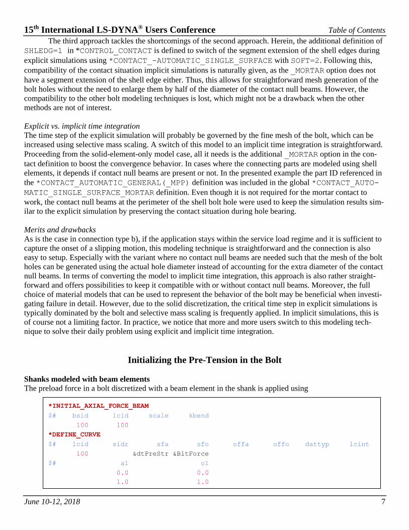
Shanks modeled with beam elements

The preload force in a bolt discretized with a beam element in the shank is applied using

*INITIAL_AXIAL_FORCE_BEAM

$# bsid lcid scale kbend

100 100

*DEFINE_CURVE

$# lcid sidr sfa sfo offa offo dattyp lcint

100 &dtPreStr &BltForce

$# a1 o1

0.0 0.0

1.0 1.0


June 10-12, 2018 8

Herein, bsid denotes the beam set ID (here 100), lcid is the load curve ID defining preload force versus

time, scale is the scale factor on load curve and kbend is an optional bending stiffness of the bolt during the

initialization phase. If the kbend=0, the bolt does not have a bending stiffness during initialization. In cases

where this is required, the user can use this feature starting with LS-DYNA versions R10. In the presented ex-

ample, a linear application of the pre-tension force BltForce is applied within dtPreStr.

The initialization phase is completed, when the load curve ends or its ordinate drops to zero. It is im-

portant to end the initialization phase before the connection is loaded in the simulation to activate the material

law of the bolt. Otherwise, the normal force will still be substituted by the prescribed pre-tension. Moreover, the

manual states, “the time duration of the ramp should produce a quasistatic response”. In practice of explicit

simulations, like for instance during a 120 ms crash event, the bolts are very often fastened within the first mil-

lisecond, which is of course far away from producing a quasistatic response. However, settings that will help to

get a quasi-static pre-tension in the bolts include sufficient damping and friction of the contact definition, appli-

cation of *DAMPING_PART_STIFFNESS with COEF=0.05 (more or less) and modeling the bolt connection

with the smallest possible gap between the parts in contact such that unnecessary travel during the pre-tension

phase is avoided.

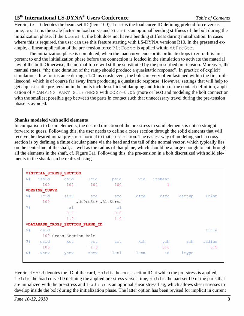
Shanks modeled with solid elements

In comparison to beam elements, the desired direction of the pre-stress in solid elements is not so straight

forward to guess. Following this, the user needs to define a cross section through the solid elements that will

receive the desired initial pre-stress normal to that cross section. The easiest way of modeling such a cross

section is by defining a finite circular plane via the head and the tail of the normal vector, which typically lies

on the centerline of the shaft, as well as the radius of that plane, which should be a large enough to cut through

all the elements in the shaft, cf. Figure 3a). Following this, the pre-tension in a bolt discretized with solid ele-

ments in the shank can be realized using

Herein, issid denotes the ID of the card, csid is the cross section ID at which the pre-stress is applied,

lcid is the load curve ID defining the applied pre-stress versus time, psid is the part set ID of the parts that

are initialized with the pre-stress and izshear is an optional shear stress flag, which allows shear stresses to

develop inside the bolt during the initialization phase. The latter option has been revised for implicit in current

*INITIAL_STRESS_SECTION

$# issid csid lcid psid vid izshear

100 100 100 100 1

*DEFINE_CURVE


100 &dtPreStr &BltStrss

$# a1 o1

0.0 0.0

1.0 1.0

*DATABASE_CROSS_SECTION_PLANE_ID

$# csid title

100 Cross Section Bolt

$# psid xct yct zct xch ych zch radius

100 -1.6 0.6 5.5

$# xhev yhev zhev lenl lenm id itype


June 10-12, 2018 9

developer versions (SVN> 123041, including R11 branch) and now allows bending stresses to develop. For ex-

plicit analysis, for backward compatibility reasons, this will be available as izshear=2 as of R11, while for

implicit izshear=1 and izshear=2 are synonymous. In the presented example, a linear application of the

pre-stress BltStrss is applied within dtPreStr.

a) b) c)

Fig. 3: a) shows the definition of the cross section plane in the shank, which is indicated by the black ring as

well as the red normal vector along the centerline of the shank. Parts b) and c) show the mesh before

and after the application of the pre-stress, respectively. It is apparent how the element with the pre-

stress application shrink until equilibrium is reached, i.e., head and nut have traveled far enough to be

in contact with the sheets.

Note how the pre-tensioning causes the bolt to shrink in Figure 3 b) and c) after the pre-stress is applied. Fol-

lowing this, the greater the gap between the head, nut and the sheets, the greater this initial shrinkage. If the el-

ements where the pre-stress is applied are not big enough to compensate this movement, they will either shrink

to very flat elements with a very small explicit time step or they will ultimately even shrink down to a plane,

which will trigger an error termination. Similar holds when modeling the shank with a beam element.

Moreover, note how the revised optional shear stress flag izshear of the LS-DYNA developer version

(SVN> 123041) influences the normal stress distribution in the bolt after the pre-stressing phase is over.

Switching on this option allows shear stresses to develop in the solid elements during the pre-stressing phase,

which leads to a more realistic distribution of the normal stresses at equilibrium, i.e., being higher at the perime-

ter and lower at the center of the cross section. Figure 4 shows the normal stress of the pre-stressed solid ele-

ments in the shank with (a) and without (b) the optional shear stress development.

a) b)

Fig. 4: Influence of the pre-stressing option izshear during the initialization phase of the shank with a pre-

stress of 0.38 GPa in an implicit simulation using LS-DYNA developer version (SVN> 123041) where

a) shows a generated homogeneous normal stress of 0.38 GPa for izshear=0 while b) was obtained

with izshear=1 leading to an inhomogeneous normal stress which averages the desired pre-stress

value of 0.38 GPa.


June 10-12, 2018 10

Finally, note that implicit simulations converge most quickly if the shank is discretized with a mesh hav-

ing only hexahedron elements. In the current LS-DYNA versions R9.2 and R10.1, there seems to be a problem

with pre-tensioning of pentahedrons elements whenever there is a gap between the connected sheets and the

bolts head or nut. This deficiency is overcome in the LS-DYNA developer version (SVN> 123041).

General rules of thumb during pre-tension initialization

In general, the time to initialize the pre-tension in the bolt should be sufficiently long such that the head and nut

of the bolt are able to establish a sufficient contact force with the connected materials, i.e., they should be in

equilibrium with the pre-tension force. The amount of time needed varies with the gap that is left between the

head or nut and the respective surfaces of the connected materials, i.e., the greater the gap, the further the parts

have to move to get in good contact with each other and the longer it will take them to do so. If the necessary

time is not given during the initialization, the bolt will not reach the desired pre-tension force when the simula-

tion continues, as there will still be movement of the head and nut until there is equilibrium with the contact

forces. Until this equilibrium is reached, the bolt will continue to contract, thereby losing its applied pre-tension

again. This effect can be seen in Figure 5, where the duration of the pre-tension application of the bolt is varied.

Following this, the gap between the head, nut and the contacting materials should be as small as possible

where an already closed gap resembles the perfect initial geometry. However, in practice this is not always pos-

sible to achieve such that a small gap is often inevitable but the user should model the bolt with the smallest

possible gap. Another problem is caused by bolts that are modeled slightly skew due to whatever reason. In

general, skew bolts should be avoided. Depending on the friction in the contact definition, skew bolts might

trigger a sliding motion of the head and nut on the sheet surfaces after pre tensioning is finished, which will in-

duce vibrations or slip of the connection.

a) Bolt modeled with spot weld beam b) bolt modeled with solid elements

Fig. 5: Different durations for pre-tension initialization in the bolt. Curves A to D are achieved with explicit

simulations while curve E is the quasi-static reference solution from an implicit simulation.It can be

seen that an application of the pre-tension in only 0.1 ms is too fast and should be avoided.

Moreover, large gaps or extremely fast pre-tension applications also introduce a lot of vibration during

the impact of the head and nut on the connected parts. In explicit simulations, this will cause stress waves that

will continue to bounce back and forth in the rest of the simulation model causing unnecessary high noise lev-

els. In implicit simulations, this impact might even cause the simulation not to converge properly. A close look

reveals that friction in the contact definition helps to dissipate that energy and to calm the system down again.

This can be greatly enhanced by applying additional damping in the initialization phase and a little bit after-

wards, too. After the system calmed down, the damping can be reduced or taken away such that the load case of

interest is not disturbed. Please note that global damping is not advised to use, if the model has an initial veloci-

ty (e.g. in car crash applications), as the global damping will slow down the whole vehicle while it is activated.

Instead, *DAMPING_PART_STIFFNESS of 5% might be more suitable solution to keep oscillations to a min-


June 10-12, 2018 11

imum. Figure 5 shows how the force in the bolt oscillates after the head and nut impact the materials to be con-

nected.

In typical models for explicit crash analysis, the bolts are modelled with the smallest possible gap and a pre-

tension initialization phase of 0.5 to 1 ms. Thus, in an explicit crash simulation, the pre-tensioning of the bolts is

easily accommodated in the whole simulation run.

Implicit models benefit from the possibility of applying larger time steps and the ability to reduce dy-

namic effects such that static equilibrium is reached, thereby fully calming down the pre-tensioned model.

However, all implicit simulations where bolts are pre-tensioned should start fully dynamic to avoid a singular

stiffness matrix while the bolt is still loose in the bolt hole. Damped Newmark time integration schemes as well

as decaying dynamic terms help to reach a quasi-static solution after the pre-tension initialization phase. Typi-

cally, this can be achieved with the following control cards, where gamma and beta govern the numerical damp-

ing of the Numark scheme and curve ID 42 starts to switch off dynamic contributions at time dtPreStr to

achieve a quasi-static solution at time 2*dtPreStress. If the simulation needs to be continued as a static simula-

tion, this is sufficient. In the case of the bolt with loads beyond the service load, a slipping motion will occur

that should be tackled by switching on the dynamic parts again. This can be done by adding a fourth coordinate

in curve ID 42 which reaches the ordinate of 1.0 after the time &tLoad. Please note that values between 0.0

and 1.0 are also permitted if one is interested to keep the system as calm as possible.

General Settings for the Implicit Models

All implicit simulations of bolt types a, b, c, and d were carried out using the same solver settings, which follow

Appendix P in LS-DYNA® Keyword Manual [8]

*CONTROL_IMPLICIT_DYNAMICS

$# imass gamma beta tdybir tdydth tdybur irate alpha

-42 0.60 0.38000

*DEFINE_CURVE


42

$# a1 o1

0.0 1.0

&dtPreStr 1.0

2.0*&dtPreStr 0.0

( &tLoad 1.0) … optional to switch dynamics back on

*CONTROL_IMPLICIT_GENERAL

$# imflag dt0 imform nsbs igs cnstn form zero_v

1 &dt0

*CONTROL_IMPLICIT_SOLUTION

$# nsolvr ilimit maxref dctol ectol rctol lstol abstol

12 6 12 1.0e-20

$# dnorm diverg istif nlprint nlnorm d3itctl cpchk

1 3 4 1

$# arcctl arcdir arclen arcmth arcdmp arcpsi arcalf arctim

$# lsmtd lsdir irad srad awgt sred


June 10-12, 2018 12

Typically, the time step size &dt0, the number of iterations ilimit and the maximum number of

stiffness matrix reformations maxref are problem specific and should be tweaked by the user to obtain the best

convergence behavior. To achieve the same level of accuracy throughout the simulation, the displacement norm

should be computed with respect to the displacement of the displacement increment of the last time step instead

of the total displacement, which is chosen using dnorm=1. To prevent premature convergence, the absolute

convergence criteria should be switched off by setting abstol to a very small number. Moreover, as shell and

solid elements are present in the example, there are translational and rotational degrees of freedom to be solved.

Following this, the nonlinear convergence norm should consider the sum of translational and rotational degrees

of freedom, i.e., no separate treatment. This is achieved by setting nlnorm=4, which scales the rotational de-

grees of freedom to account for their different units based on a characteristic element size that is calculated in-

ternally. The remaining settings of nlprint and d3itctl are for debugging purposes to be able to identify

convergence problems and can be left blank in smoothly running decks.

Another important setting addresses the automatic control of the time step size, which may depend on

convergence, as well as the definition of so-called key points. The latter are necessary to define important points

in time that are actually reached during the simulation, e.g. the end of the pre-tensioning phase &dtPreStrss

or the beginning of the loading &tLoad. In explicit simulations, this is usually not an issue, as the time steps

are small enough such that “overshooting” of key points is of negligible magnitude. In implicit simulations,

time steps are larger and the overshooting may significantly miss the end of the pre-tensioning phase or the on-

set of a subsequent load. For the presented example, auto time stepping as well as the key points are defined by

Herein, the optimal number of iterations is defined by the window itopt=40 +/- itewin=10. If the

needed iterations to converge lie above or below this window, the initial time step size &dt0 is decreased or

increased, respectively, until the boundaries dtmin or dtmax are reached. Following this, the maximum size

dtmax of the time step can be defined by a curve definition, to alter the size during the simulation. In the pre-

sented example, this is done by the curve with ID=24 where the points of this curve simultaneously define the

key points in time, which are needed for accurate results.

Example for all four Bolt Connections

The input decks of the presented four examples for friction bolt connections can be downloaded on our LS-

DYNA examples page [9]. The example consists of a M10 bolt of grade 8.8, which connects two sheets of ma-

terial where one sheet is modeled using shell elements and the other using hexahedron solid elements. The

models were tested with the official LS-DYNA MPP R9.2 release and it has been noted that the current LS-

DYNA R10 and R10.1 releases still have some issues with the implicit models. All four connection types are

modeled such that their input decks run with the same control cards in explicit and implicit.

Following this, all examples are controlled by the keyword file main.k where the user can choose to

include the needed control cards for an explicit or an implicit solution, i.e. control_explicit.k or con-

*CONTROL_IMPLICIT_AUTO

$# iauto iteopt itewin dtmin dtmax dtexp kfail kcycle

1 40 10 -24

*DEFINE_CURVE


24

$# a1 o1

&dtPreStrss &dtMax

&tLoad &dtMax


June 10-12, 2018 13

trol_implicit.k, respectively. The second important include to choose from is the definition of one of the

four bolt types, which contains their node, element, material, section, part and set definitions as well as the ini-

tial stress, boundary and loading conditions. These include files are bolted_connection_{a,b,c,d}.k.

To switch between bolt models as well as implicit and explicit simulations, the user should open main.k using

a text editor and remove the comments of the respective lines in the top part of the file.

Summary

The paper provides four different modeling approaches for friction grip bolts using LS-DYNA with explicit and

implicit time integration. Following this, the well-known modeling strategies in explicit have been explained,

pitfalls have been identified and necessary changes to switch to implicit applications have been presented. In

this process, we recognized some shortcomings and provided solutions to most of them. With the aid of the pro-

vided examples, users should be able to switch successfully to implicit time integration with minimal changes to

their existing models. Moreover, it should also help to follow the one-model-strategy of LSTC when setting up

new models.

References

[1] Sonnenschein, U.: Modelling of bolts under dynamic loads. Proceedings of the 7th LS-DYNA Forum,

Bamberg, Germany, 2008.

[2] Lou, K.-A. and Perciballi, W.: Finite element modeling of preloaded bolt under static three-point bending

load. Proceedings of the 10th International LS-DYNA Conference, Detroit, USA, 2008.

[3] Narkhede, S.; Lokhande, N.; Gangani, B. and Gadekar, G.: Bolted joint representation in LS-DYNA® to

model bolt pre-stress and bolt failure characteristics in crash simulations. Proceedings of the 11th Interna-

tional LS-DYNA Conference, Detroit, USA, 2010.

[4] Meyer, M.: Development of an improved screw model at Faurecia. Proceedings of the 11th European LS-

DYNA Conference, Strassburg, France, 2011.

[5] Hadjioannou, M.; Stevens, D. and Barsotti, M.: Development and validation of bolted connection modeling

in LS-DYNA® for large vehicle models. Proceedings of the 14th International LS-DYNA Conference, De-

troit, USA, 2016.

[6] Koehler, M.; Fish, G. and Braughler, R.: Development of accurate finite element models and testing proce-

dures for bolted joints in large caliber gun weapon systems. Proceedings of the 11th European LS-DYNA

Conference, Salzburg, Austria, 2017.

[7] Erhart, T. and Borrvall, T.: Drilling rotation constraint for shell elements in implicit and explicit analysis.

Proceedings of the 9th European LS-DYNA Conference, Manchester, UK, 2013.

[8] LS-DYNA® Keyword User’s Manual, Volumes I-II, Livermore Software Technology Corporation (LSTC),

2018.

[9] Karajan, N.: LS-DYNA input decks for friction grip bolts,

http://www.dynaexamples.com/connections/bolts

http://www.dynaexamples.com/connections/bolts

Modeling bolts in LS-DYNA© using explicit and implicit time ...

Documents

Transcript of Modeling bolts in LS-DYNA© using explicit and implicit time ...