Pullout test of rock bolts at the Lima Hydropower station

IN DEGREE PROJECT CIVIL ENGINEERING AND URBAN MANAGEMENT,SECOND CYCLE, 30 CREDITS

, STOCKHOLM SWEDEN 2016

Pullout test of rock bolts at the Lima Hydropower station-Assessment of the test method

JAKOB LJUNGBERG

KTH ROYAL INSTITUTE OF TECHNOLOGYSCHOOL OF ARCHITECTURE AND THE BUILT ENVIRONMENT

Pullout test of rock bolts at the LimaHydropower station- Assessment of the test method

Jakob Ljungberg

September 2016TRITA-BKN. Master Thesis 499, 2016ISSN 1103-4297,ISRN KTH/BKN/EX–499–SE

c©Jakob Ljungberg 2016Cover photo, Rikard HellgrenRoyal Institute of Technology (KTH)Department of Civil and Architectural EngineeringDivision of Concrete StructuresStockholm, Sweden, 2016

Abstract

During construction of dams, rock bolts are in general installed in the interfacebetween concrete and rock as an extra safety measure against overturning failure.These bolts are however not allowed to be taken into consideration for the stabilitycalculations of large dams. New standards and new design criterias have increasedthe requirements of the safety of the old dams, leading to a need for expensiverehabilitation and strengthening. It is possible that consideration of these boltsin stability calculations may lead to money being saved. In order to do so moreinformation about the long term strength of these bolts is needed. One way ofgetting this information has been the destructive testing of old dugout bolts foundduring reconstruction works. At the Lima hydropower station in Sweden, this kindof testing was made. The test rig used had a design where a piston pressed downon the rock around the bolt in order to pull it out. The question was raised if thiscould affect the failure load of the bolt. In this thesis, an attempt was made toanswer this question using finite element methods.

Models of a rock bolt was made in Abaqus, where one model included the piston andone where it was not. The connection between the bolt and the rock was modelledwith nonlinear springs and friction, and the results were then compared between thecases and with experimental data.

The results showed that the resulting force-deformation curves may be affected bythe piston in cases where the dominant failure mode was adhesive failure, whichwould influence failure loads and deformations. Since so little was known about theproperties of the rock and grout at Lima however, it is difficult to say to whichextent the test rig has affected these results.

iii

Sammanfattning

Vid byggandet av dammar placeras ofta bergförankringar under hela dammen somen extra säkerhetsåtgärd för att förhindra stjälpning. Dessa förankringar fick dockinte räknas med i stabilitetsberäkningarna för stora dammar. Med nya standarderoch nya riktlinjer har också kraven på äldre dammar höjts och lett till att de skullebehöva renoveras för stora summor. Om dessa bergförankringar skulle få användasi stabilitetsberäkningarna så skulle pengar kunna sparas. För att få göra det såbehövs mer information om dessa bultars styrka. Ett sätt att få den informationenär genom destruktiva tester av utgrävda förankringar som funnits vid renoveringar.Vid Limas vattenkraftsstation i Sverige har sådana tester gjorts. Testriggen hadeen konstruktion där en kolv tryckte ner på berget runt förankringen för att draupp den. Frågan ställdes om detta kunde påverka bultens brottlast. I den häruppsatsen har ett försök gjorts för att svara på den frågan genom användandet avfinita element-metoder.

Modeller av bergförankringen simulerades i Abaqus, en där kolven fanns med, och enutan. Anslutningen mellan bulten och berget modellerades med ickelinjära fjädraroch friktion, och resultaten jämfördes sedan mellan modellerna och mot försöksdata.

Resultaten visade att kraft-deformations-kurvorna kunde påverkas av kolven dåbrottet förväntades i vidhäftningen och orsaka olika brottlaster och deformationer.Eftersom så lite var känt om berg- och bruksegenskaperna vid Lima så är det docksvårt att säga hur mycket som resultaten där har påverkats.

v

Preface

The research presented in this thesis was carried out at the Division of ConcreteStructures, Department of Civil and Architectural Engineering at the Royal Institueof Technology (KTH). The project was initiated by Dr. Richard Malm, who alsosupervised the project.

The research was carried out as a part of "Swedish Hydropower Centre - SVC". SVChas been established by the Swedish Energy Agency, Elforsk and Svenska Kraftnättogether with Luleå University of Technology, KTH Royal Institute of Technology,Chalmers University of Technology and Uppsala University. www.svc.nu.

I would like to express my sincerest gratitude to my supervisor Richard Malm forhis support and help during this project.

A special thanks also to Doctoral Student Rikard Hellgren for his advise and helpwith the numerical analyses.

Stockholm, June 2016

Jakob Ljungberg

vii

Contents

Abstract iii

Sammanfattning v

Preface vii

1 Introduction 1

1.1 Background . . . . . . . . . . . . . . . . . . . . . . . . . . . . . . . . 1

1.2 Aims and scope . . . . . . . . . . . . . . . . . . . . . . . . . . . . . . 1

1.3 Structure of the thesis . . . . . . . . . . . . . . . . . . . . . . . . . . 2

2 Concrete anchors 3

2.1 Failure modes . . . . . . . . . . . . . . . . . . . . . . . . . . . . . . . 3

2.2 Load capacity of anchors . . . . . . . . . . . . . . . . . . . . . . . . . 4

2.2.1 Steel failure . . . . . . . . . . . . . . . . . . . . . . . . . . . . 4

2.2.2 Bond failure . . . . . . . . . . . . . . . . . . . . . . . . . . . . 5

2.2.3 Concrete cone failure . . . . . . . . . . . . . . . . . . . . . . . 7

2.2.4 The influence of input parameters on failure modes . . . . . . 9

2.3 Previous tests of rock bolts . . . . . . . . . . . . . . . . . . . . . . . . 10

2.3.1 50-year old bolts at the Hotagen regulating dam . . . . . . . . 11

2.3.2 Norwegian tests of new grouted rock bolts . . . . . . . . . . . 11

3 Non-linear material behaviour 13

3.1 Concrete . . . . . . . . . . . . . . . . . . . . . . . . . . . . . . . . . . 13

3.1.1 Tensile properties . . . . . . . . . . . . . . . . . . . . . . . . . 13

ix

3.1.2 Compressive properties . . . . . . . . . . . . . . . . . . . . . . 15

3.2 Steel . . . . . . . . . . . . . . . . . . . . . . . . . . . . . . . . . . . . 15

4 Benchmark examples 17

4.1 Notched Beam . . . . . . . . . . . . . . . . . . . . . . . . . . . . . . . 17

4.2 Headed bolt anchor . . . . . . . . . . . . . . . . . . . . . . . . . . . . 20

4.3 Bond failure . . . . . . . . . . . . . . . . . . . . . . . . . . . . . . . . 25

5 Load capacity of rock bolts at Lima hydropower station 29

5.1 Field test . . . . . . . . . . . . . . . . . . . . . . . . . . . . . . . . . 29

6 Numerical model of the Lima bolts 35

6.1 Numerical model . . . . . . . . . . . . . . . . . . . . . . . . . . . . . 35

6.1.1 Weak grout and low strength bolt . . . . . . . . . . . . . . . . 37

6.1.2 Higher strength grout and bolt . . . . . . . . . . . . . . . . . 38

6.1.3 Weak grout and stronger strength bolt . . . . . . . . . . . . . 39

7 Conclusions 43

7.1 Discussion . . . . . . . . . . . . . . . . . . . . . . . . . . . . . . . . . 43

7.2 Further research . . . . . . . . . . . . . . . . . . . . . . . . . . . . . . 44

Bibliography 45

x

Chapter 1

Introduction

1.1 Background

During the construction of dams, in many cases the structure has been anchored tothe bedrock with grouted anchors. This has been done as an extra safety precaution,despite that there is no reliable way to determine the strength of the anchors. Dueto this, the anchors have not been included in the design calculations determiningthe safety factors for overturning and sliding failure modes.

The requirements of safety factors and design standards have increased, meaningthat many old dams would need to be modified at a large cost. However, if theanchor strength could be determined and considered when calculating the safetyfactors, then it may be possible to use the dams without any changes.

An effort has therefore been made to test old bolts when possible for example duringredesign or renovation of old dams, in order to learn more about their state andgather data that could be used to find methods to determine the strength of oldanchors. One of these possibilities was during the redesign of the Lima Hydropowerstation. In these tests, a rig was used that presses down on the rock around the boltin order to pull the bolt upwards. This does not only hinder a rock cone failure, butcould also affect the load capacity of the bolt.

1.2 Aims and scope

The aims of this master’s thesis is to study if it is possible that the test rig affectsthe load capacity. The hypothesis is that the cylinder pressing down on the rock willintroduce stresses that pinches the bolt and thereby results in higher failure load.

This is studied with the use of finite element models that includes nonlinear be-haviour of grout, rock and rock bolts in order to be able to capture the relevantfailure modes.

1

CHAPTER 1. INTRODUCTION

1.3 Structure of the thesis

The thesis will begin with some background in the "Concrete anchors"-chapter anddescriptions of the different failure modes of concrete/rock anchors.

After this, the "Non-linear material behaviour"- behaviour will go into the behaviourof non-linear materials and describe how the input values were chosen for the laterFE simulations.

In the next chapter, chapter 4 some benchmark examples will be made in orderto make sure that the final FE models will be able to simulate the behaviour ofconcrete, grout and steel realistically. In this chapter one example will be used tocheck the tensile properties of concrete, one to see if a cone failure can be simulated,and one to see how adhesion failure can be simulated.

Chapter 5 will describe the bolts at Lima and the tests that have been made there.

After this in chapter ref:chapter6 the FE modelling of bolts similar in design tothe Lima bolts, but with different properties, will be presented. This chapter willalso contain the results of these simulations.

Finally the conclusions of the thesis will be presented in chapter 7, along withsuggestions for further research.

2

Chapter 2

Concrete anchors

This chapter will contain some information about bonded anchors, aswell as theirfailure modes and when these occur.

A bonded anchor consists of a steel rod that is post-installed into a hole drilled intoa concrete element or rock mass. Bonded anchors give the possibility to transfertensile and shear loads from the steel rod into the base material (Mahrenholtz et al.,2015). In this report only the tensile properties are relevant. There is currently littleinformation about the degradation of the strength and reliability of old rock boltsthat have been embedded in dams. To date there have only been two test seriesmade in Sweden (Hellgren et al., 2015b). The first one was conducted in 2008, see(Larsson, 2008), and the second one is the Lima-tests (Hellgren et al., 2015b). InNorway some additional tests have been made, see for example Thomas-Lepine andLia (2014). In many of the cases, the rock bolts have been in good condition evenafter long periods of time.

2.1 Failure modes

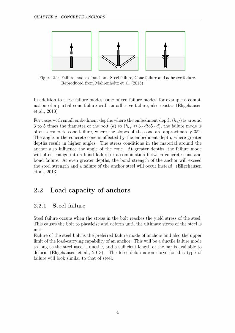
In the case of a grouted anchor in the bedrock/concrete, there are three main failurecategories as seen in Figure 2.1. These are:

• Failure of the steel

• Rock/Concrete cone failure

• Adhesive failure

– Failure in the rock/concrete-grout interface

– Failure in the grout-steel interface

3

CHAPTER 2. CONCRETE ANCHORS

Figure 2.1: Failure modes of anchors. Steel failure, Cone failure and adhesive failure.Reproduced from Mahrenholtz et al. (2015)

In addition to these failure modes some mixed failure modes, for example a combi-nation of a partial cone failure with an adhesive failure, also exists. (Eligehausenet al., 2013)

For cases with small embedment depths where the embedment depth (hef ) is around3 to 5 times the diameter of the bolt (d) so (hef ≈ 3 · dto5 · d), the failure mode isoften a concrete cone failure, where the slopes of the cone are approximately 35◦.The angle in the concrete cone is affected by the embedment depth, where greaterdepths result in higher angles. The stress conditions in the material around theanchor also influence the angle of the cone. At greater depths, the failure modewill often change into a bond failure or a combination between concrete cone andbond failure. At even greater depths, the bond strength of the anchor will exceedthe steel strength and a failure of the anchor steel will occur instead. (Eligehausenet al., 2013)

2.2 Load capacity of anchors

2.2.1 Steel failure

Steel failure occurs when the stress in the bolt reaches the yield stress of the steel.This causes the bolt to plasticize and deform until the ultimate stress of the steel ismet.Failure of the steel bolt is the preferred failure mode of anchors and also the upperlimit of the load-carrying capability of an anchor. This will be a ductile failure modeas long as the steel used is ductile, and a sufficient length of the bar is available todeform (Eligehausen et al., 2013). The force-deformation curve for this type offailure will look similar to that of steel.

4

2.2. LOAD CAPACITY OF ANCHORS

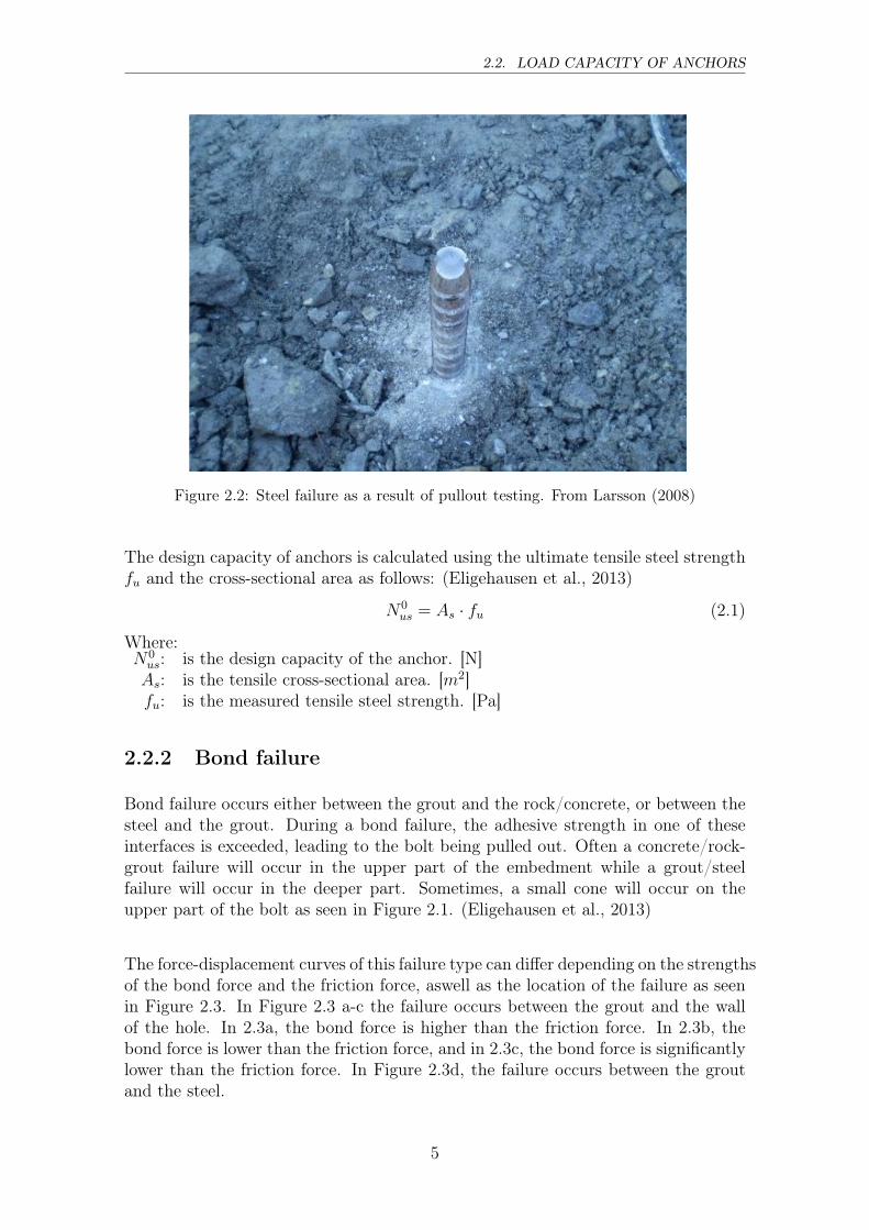
Figure 2.2: Steel failure as a result of pullout testing. From Larsson (2008)

The design capacity of anchors is calculated using the ultimate tensile steel strengthfu and the cross-sectional area as follows: (Eligehausen et al., 2013)

N0us = As · fu (2.1)

Where:N0

us: is the design capacity of the anchor. [N]As: is the tensile cross-sectional area. [m2]fu: is the measured tensile steel strength. [Pa]

2.2.2 Bond failure

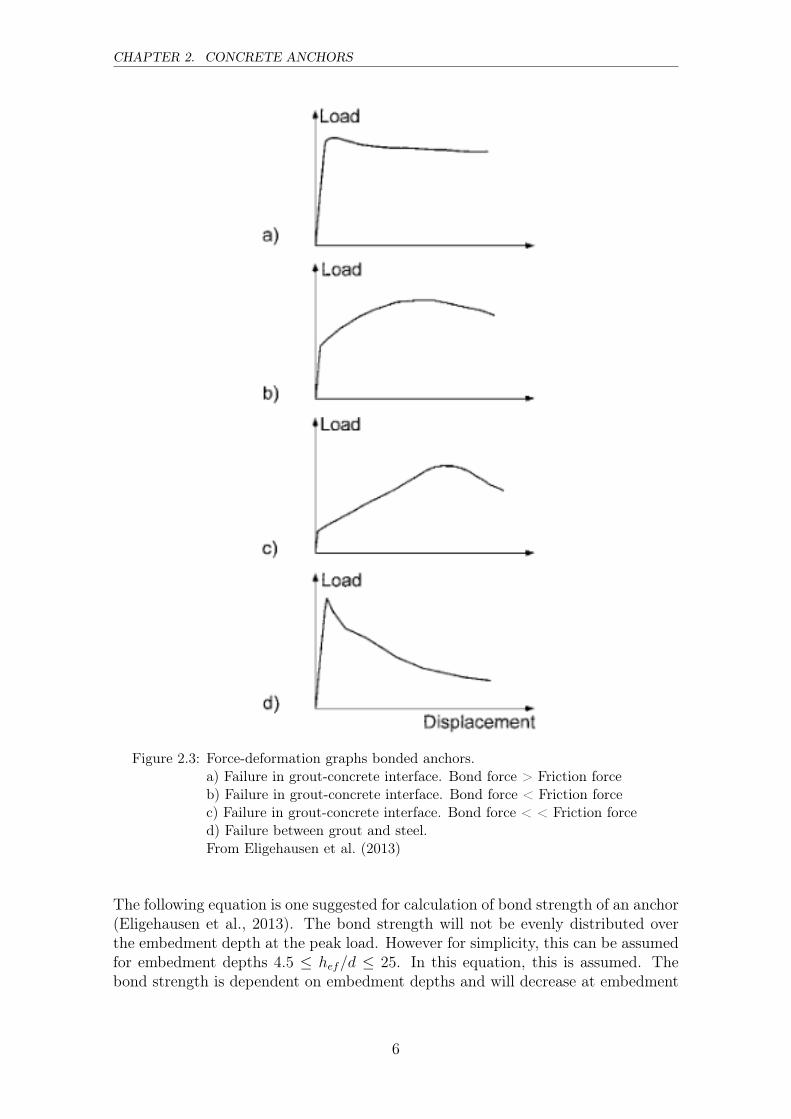
Bond failure occurs either between the grout and the rock/concrete, or between thesteel and the grout. During a bond failure, the adhesive strength in one of theseinterfaces is exceeded, leading to the bolt being pulled out. Often a concrete/rock-grout failure will occur in the upper part of the embedment while a grout/steelfailure will occur in the deeper part. Sometimes, a small cone will occur on theupper part of the bolt as seen in Figure 2.1. (Eligehausen et al., 2013)

The force-displacement curves of this failure type can differ depending on the strengthsof the bond force and the friction force, aswell as the location of the failure as seenin Figure 2.3. In Figure 2.3 a-c the failure occurs between the grout and the wallof the hole. In 2.3a, the bond force is higher than the friction force. In 2.3b, thebond force is lower than the friction force, and in 2.3c, the bond force is significantlylower than the friction force. In Figure 2.3d, the failure occurs between the groutand the steel.

5


Figure 2.3: Force-deformation graphs bonded anchors.a) Failure in grout-concrete interface. Bond force > Friction forceb) Failure in grout-concrete interface. Bond force < Friction forcec) Failure in grout-concrete interface. Bond force < < Friction forced) Failure between grout and steel.From Eligehausen et al. (2013)

The following equation is one suggested for calculation of bond strength of an anchor(Eligehausen et al., 2013). The bond strength will not be evenly distributed overthe embedment depth at the peak load. However for simplicity, this can be assumedfor embedment depths 4.5 ≤ hef/d ≤ 25. In this equation, this is assumed. Thebond strength is dependent on embedment depths and will decrease at embedment

6


depths hef > 9d (Eligehausen et al., 2013). The bond strength τu depends on thegrout used, but is also influenced by the moisture conditions of the drill hole, thedrill technique, the degree to which the hole is cleaned and the temperature of thematerials. For bonded anchors with a ratio between the drill hole and the anchorrod of d0/d ≤ 1.5, bond strength is primarily a function of mortar type. Since thevalue is highly affected by local conditions, it is determined experimentially. Thebond strength is not significantly dependent on rod diameter, but is affected by thestrength of the concrete. Concrete of higher strength will have smoother contactsurface, reducing the bond strength. However, according to Eurocode 2: EN 1992-1-1 (2004) it can be expected that bond strength obtained from concrete tests with acompressive strength of fc ≈ 20MPa are also valid for concretes up to class C50/60.For embedment depths 4.5 ≤ hef/d ≤ 20, diameters d ≤ 50 mm and bond areasπ · d · hef ≤ 55000 mm2 the following equation will give a results with a sufficientaccuracy, independent on failure type (Eligehausen et al., 2013) .

N0u = π · d · hef · τu (2.2)

Where:N0

u : is the design capacity of the anchor. [Pa]d: is the diameter of the bolt. [m]

hef : is the embedment depth. [m]τu: is the bond strength. [Pa]

2.2.3 Concrete cone failure

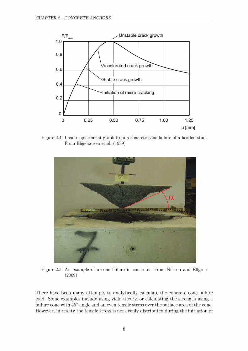
In the concrete cone failure mode, cracks will start to develop from the bottom ofthe bolt and leading to a cone shaped piece breaking off with the anchor, see Figure2.5. During this type of failure the full tensile capacity of the concrete is utilised.Cone failure is often seen as a relatively non-ductile failure mode. An exampleof a load-displacement curve for this type of failure with a headed anchor can beseen in Figure 2.4. The failure mode is common in expansion anchors and in headedstuds and undercut anchors with an adequately large bearing surface. In non-headedanchors this failure is uncommon unless the embedment depth is small. (Eligehausenet al., 2013)

7


Figure 2.4: Load-displacement graph from a concrete cone failure of a headed stud.From Eligehausen et al. (1989)

Figure 2.5: An example of a cone failure in concrete. From Nilsson and Elfgren(2009)

There have been many attempts to analytically calculate the concrete cone failureload. Some examples include using yield theory, or calculating the strength using afailure cone with 45◦ angle and an even tensile stress over the surface area of the cone.However, in reality the tensile stress is not evenly distributed during the initiation of

8


a cone breakout and the concrete does not have the elasto-plastic properties assumedin the yield line theory. To be able to make a realistic analysis of the concrete conefailure mode, the non-linear behaviour of the tensioned concrete needs to be takeninto account. Finite element analysis is one method to get reasonable predictionsand results of the concrete cone failure loads. The quickest way to assess the failureloads is to use the empirically derived equations which encompass theoretical models.The CC (Concrete capacity) method is one of these methods. (Eligehausen et al.,2013) With this, the failure load can be calculated as follows: (Mahrenholtz et al.,2015)

NRd,c = k · f 0.5ck,cyl · h1.5ef (2.3)

Where:NRd,c: is the design capacity of the anchor. [MN]

k: is an empirically determined factor which is 7.7 for cracked concrete and 11for uncracked concrete.

fck,cyl: is the characteristic concrete compressive strength using test cylinderswith a diameter of 150 mm and a length of 300 mm. [MPa]

hef : is the embedment depth. [m]

2.2.4 The influence of input parameters on failure modes

As seen in the formulas above, the anchor strength is affected by a series of factors.By modifying these factors, different failure types will occur.

As an example it can be mentioned that according to the Norwegian guidelines forconcrete dams the characteristic strength of the mortar should be at least 3.0 MPa(NVE, 2005) and that a commonly used minimum value of the characteristic yieldstress of the steel bolts in concrete dams is 370 MPa (Hellgren et al., 2015b).

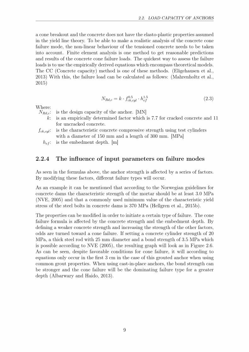
The properties can be modified in order to initiate a certain type of failure. The conefailure formula is affected by the concrete strength and the embedment depth. Bydefining a weaker concrete strength and increasing the strength of the other factors,odds are turned toward a cone failure. If setting a concrete cylinder strength of 20MPa, a thick steel rod with 25 mm diameter and a bond strength of 3.5 MPa whichis possible according to NVE (2005), the resulting graph will look as in Figure 2.6.As can be seen, despite favorable conditions for cone failure, it will according toequations only occur in the first 3 cm in the case of this grouted anchor when usingcommon grout properties. When using cast-in-place anchors, the bond strength canbe stronger and the cone failure will be the dominating failure type for a greaterdepth (Albarwary and Haido, 2013).

9


Figure 2.6: Force-displacement diagram in favour of cone failure. Force in [kN] anddisplacement in [m]

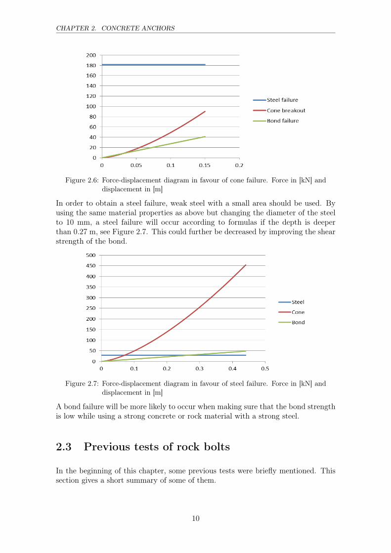
In order to obtain a steel failure, weak steel with a small area should be used. Byusing the same material properties as above but changing the diameter of the steelto 10 mm, a steel failure will occur according to formulas if the depth is deeperthan 0.27 m, see Figure 2.7. This could further be decreased by improving the shearstrength of the bond.

Figure 2.7: Force-displacement diagram in favour of steel failure. Force in [kN] anddisplacement in [m]

A bond failure will be more likely to occur when making sure that the bond strengthis low while using a strong concrete or rock material with a strong steel.

2.3 Previous tests of rock bolts

In the beginning of this chapter, some previous tests were briefly mentioned. Thissection gives a short summary of some of them.

10

2.3. PREVIOUS TESTS OF ROCK BOLTS

2.3.1 50-year old bolts at the Hotagen regulating dam

In 2008, the Hotagen regulating dam, located at Hotagssjön in Jämtland, Sweden,was demolished and rebuilt because of Alkali silicone reaction-damages that had leadto large cracks in the dam. During this reconstruction the opportunity was givento investigate and test the old rock bolts in order to learn more of the propertiesof these bolts. Of 21 bolts found, 3 were chosen for tensile testing. All steel barslooked to be in good condition and no corrosion was found. The rock quality wasfound to be poor and during the testing, the test rig would sink into the rock. Thebolts had been drilled to a depth of 3 meters in to the rock and were embedded 0.5meters in the concrete. The tests were done using a test rig that used a piston thatpressed down on the rock face around the bolt in order to pull the bolt upward.

All three bolts failed by yielding of the steel, and all three well exceeded their the-oretical tensile strength. (Larsson, 2008)

Figure 2.8: A principal sketch of the rock bolts at the Hotagen regulating dam. FromLarsson (2008)

2.3.2 Norwegian tests of new grouted rock bolts

In Norway, some relevant tests were carried out in 2012. The goal was to verifyearlier results showing that rock bolts were in fact much stronger than previouslyassumed and to start developing a new design method. In this test 50 grouted steelbolts were tested. In a previous test by Lars K. Neby in 2011 an additional 18bolts had been tested. Both these tests were made in the same limestone quarryof Verdalskalk, but in different places. The intact rock in this area had a uniaxialcompressive strength of 90 MPa, but the rock mass rating (RMR) varied between 20and 90. The depth varied between 0.1 and 1 meter. The testing was done after themortar had dried for 13 days in cold weather. An excavator with a lifting capacity of20 tons was used for the tests. It was placed a distance of three meters from the boltsin order to not affect the results. The force-deformation data was obtained using a

11


dynamometer and laser measurements. The results showed that all bolts except 6,which were in very poor rock mass with loose blocks, had a capacity greater than 88kN (180 MPa). The mortar was not dry enough which affected many of the bolts.(Thomas-Lepine, 2012) (Thomas-Lepine and Lia, 2014)

Figure 2.9: The test procedure using an excavator. From Thomas-Lepine (2012)

12

Chapter 3

Non-linear material behaviour

This chapter will explain some of the background of the non-linear material modelsthat will later be used in the analyses. It will also describe how the non-linearmaterial curves are made from the material properties.For concrete, the material properties will be described according to Eurocode 2: EN1992-1-1 (2004). For steel, BSK 07 (2007) has been chosen instead, because of itsmore detailed curve.

3.1 Concrete

Concrete is a material that has very different behaviours in tension and compression.Concrete has its strength in compression, and is relatively weak in tension. Thefailure modes also differ between cracking and crushing. The concrete propertiesused in these examples is a C30/37 concrete according to Eurocode 2: EN 1992-1-1(2004). The fracture energy has been calculated from du beton (2013)

Table 3.1: Example properties for concrete.

Young’s modulus 32 GPaTensile strength (Ft) 2.9 MPaCompressive strength (fc) 38 MPaεcu 0.0035ε1 0.002Fracture energy (Gf ) 140.5Nm/m2

3.1.1 Tensile properties

There are generally three ways to describe the softening curves of concrete in tension.There is the linear, bilinear and exponential which all vary in accuracy and simplicity,

13

CHAPTER 3. NON-LINEAR MATERIAL BEHAVIOUR

see Figure 3.1. The exponential comes closest to the actual failure curves, while thelinear is the simplest. The best curve depends on the level of accuracy needed.

Figure 3.1: Normalized plot of various softening laws, reproduced from Hofstetterand Meschke (2011).

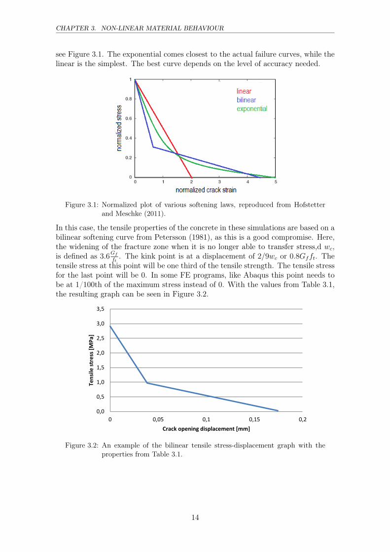
In this case, the tensile properties of the concrete in these simulations are based on abilinear softening curve from Petersson (1981), as this is a good compromise. Here,the widening of the fracture zone when it is no longer able to transfer stress,d wc,is defined as 3.6Gf

ft. The kink point is at a displacement of 2/9wc or 0.8Gfft. The

tensile stress at this point will be one third of the tensile strength. The tensile stressfor the last point will be 0. In some FE programs, like Abaqus this point needs tobe at 1/100th of the maximum stress instead of 0. With the values from Table 3.1,the resulting graph can be seen in Figure 3.2.

0,0

0,5

1,0

1,5

2,0

2,5

3,0

3,5

0 0,05 0,1 0,15 0,2

Ten

sile

str

ess

[M

Pa]

Crack opening displacement [mm]

Figure 3.2: An example of the bilinear tensile stress-displacement graph with theproperties from Table 3.1.

14

3.2. STEEL

3.1.2 Compressive properties

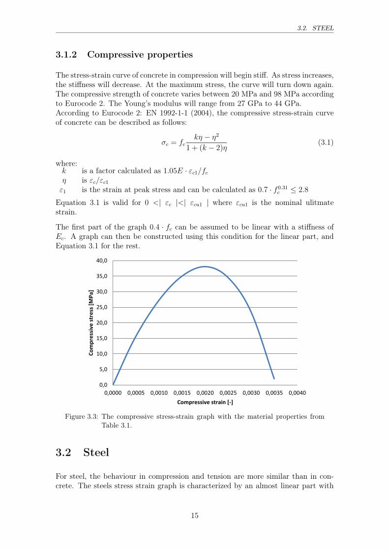
The stress-strain curve of concrete in compression will begin stiff. As stress increases,the stiffness will decrease. At the maximum stress, the curve will turn down again.The compressive strength of concrete varies between 20 MPa and 98 MPa accordingto Eurocode 2. The Young’s modulus will range from 27 GPa to 44 GPa.According to Eurocode 2: EN 1992-1-1 (2004), the compressive stress-strain curveof concrete can be described as follows:

σc = fckη − η2

1 + (k − 2)η(3.1)

where:k is a factor calculated as 1.05E · εc1/fcη is εc/εc1ε1 is the strain at peak stress and can be calculated as 0.7 · f 0.31

c ≤ 2.8

Equation 3.1 is valid for 0 <| εc |<| εcu1 | where εcu1 is the nominal ulitmatestrain.

The first part of the graph 0.4 · fc can be assumed to be linear with a stiffness ofEc. A graph can then be constructed using this condition for the linear part, andEquation 3.1 for the rest.

0,0

5,0

10,0

15,0

20,0

25,0

30,0

35,0

40,0

0,0000 0,0005 0,0010 0,0015 0,0020 0,0025 0,0030 0,0035 0,0040

Co

mp

ress

ive

str

ess

[M

Pa]

Compressive strain [-]

Figure 3.3: The compressive stress-strain graph with the material properties fromTable 3.1.

3.2 Steel

For steel, the behaviour in compression and tension are more similar than in con-crete. The steels stress strain graph is characterized by an almost linear part with

15

CHAPTER 3. NON-LINEAR MATERIAL BEHAVIOUR

high stiffness, until a point where plastization starts to occur. After som deforma-tion, the steel will be able to take more load again until the ultimate failure load.

For this graph, the input values for steel are based on a curve from BSK 07 (2007).Here the curve is determined by these formulas as seen in Figure 3.4.

Table 3.2: Example properties for steel.

Young’s modulus, E 200 GPaYield strength, fy 460 MPaUltimate strength, fu 645 MPaUltimate elongation, A 0.21mm/mm

(1) : ε1 = (fy/E)(2) : ε2 = 0.025− 5(fu/E)(3) : ε3 = 0.02 + 50(fu − fy/E)(4) : ε4 = 0.6A

0

100

200

300

400

500

600

700

0 0,02 0,04 0,06 0,08 0,1 0,12 0,14

fud

yd

(1)(2) (3)

f

(4)

Figure 3.4: The stress-strain graph for steel using the values from Table 3.2.

16

Chapter 4

Benchmark examples

In order to calibrate the finite element calculations to ensure accurate results in theproject and to make sure that the different damage mechanisms could be simulatedwell enough, a series of verification tests were made. Three benchmark exampleswere modelled in Abaqus 6.14, and the results were compared to results from realtests. These were picked with the failure modes of rock anchors in mind.

4.1 Notched Beam

The notched beam test was used since it is a good example to examine the tensileproperties of concrete. Since the compressive strength of concrete is far greaterthan the tensile strength, bending will lead to a pure tension failure at the crackopening. By adding the notch to the beam, the failure will also occur in a veryspecific and isolated point. The model was made in Abaqus and compared to thereal experimental results found in Petersson (1981). The material properties werethe same as used in the experiments, see Table 4.1, and the geometry can be seenin Figure 4.1.

Table 4.1: Material properties.

Density 2400kgYoung’s Modulus 30GPaPoisson’s ratio 0.2Compressive strength 30 MPaTensile strength 3.33 MPaFracture energy 137Nm/m2

17

CHAPTER 4. BENCHMARK EXAMPLES

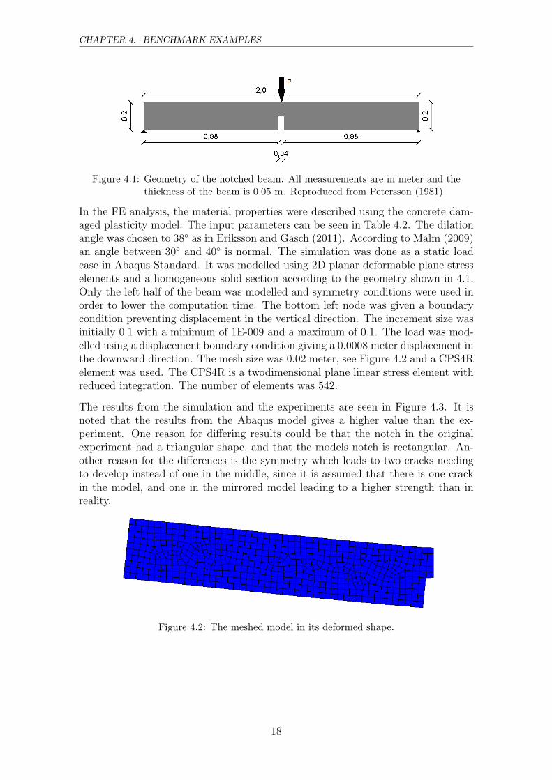
Figure 4.1: Geometry of the notched beam. All measurements are in meter and thethickness of the beam is 0.05 m. Reproduced from Petersson (1981)

In the FE analysis, the material properties were described using the concrete dam-aged plasticity model. The input parameters can be seen in Table 4.2. The dilationangle was chosen to 38◦ as in Eriksson and Gasch (2011). According to Malm (2009)an angle between 30◦ and 40◦ is normal. The simulation was done as a static loadcase in Abaqus Standard. It was modelled using 2D planar deformable plane stresselements and a homogeneous solid section according to the geometry shown in 4.1.Only the left half of the beam was modelled and symmetry conditions were used inorder to lower the computation time. The bottom left node was given a boundarycondition preventing displacement in the vertical direction. The increment size wasinitially 0.1 with a minimum of 1E-009 and a maximum of 0.1. The load was mod-elled using a displacement boundary condition giving a 0.0008 meter displacement inthe downward direction. The mesh size was 0.02 meter, see Figure 4.2 and a CPS4Relement was used. The CPS4R is a twodimensional plane linear stress element withreduced integration. The number of elements was 542.

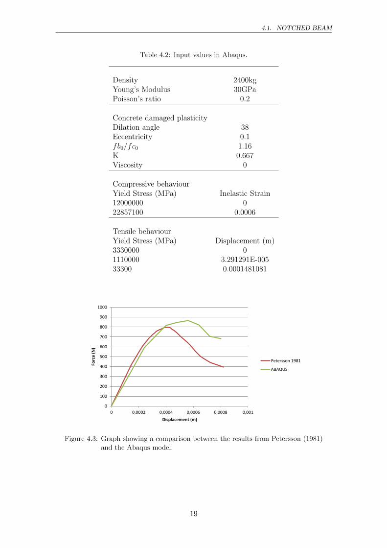
The results from the simulation and the experiments are seen in Figure 4.3. It isnoted that the results from the Abaqus model gives a higher value than the ex-periment. One reason for differing results could be that the notch in the originalexperiment had a triangular shape, and that the models notch is rectangular. An-other reason for the differences is the symmetry which leads to two cracks needingto develop instead of one in the middle, since it is assumed that there is one crackin the model, and one in the mirrored model leading to a higher strength than inreality.

Figure 4.2: The meshed model in its deformed shape.

18

4.1. NOTCHED BEAM

Table 4.2: Input values in Abaqus.

Density 2400kgYoung’s Modulus 30GPaPoisson’s ratio 0.2

Concrete damaged plasticityDilation angle 38Eccentricity 0.1fb0/fc0 1.16K 0.667Viscosity 0

Compressive behaviourYield Stress (MPa) Inelastic Strain12000000 022857100 0.0006

Tensile behaviourYield Stress (MPa) Displacement (m)3330000 01110000 3.291291E-00533300 0.0001481081

0

100

200

300

400

500

600

700

800

900

1000

0 0,0002 0,0004 0,0006 0,0008 0,001

Force(N)

Displacement (m)

Petersson 1981

ABAQUS

Figure 4.3: Graph showing a comparison between the results from Petersson (1981)and the Abaqus model.

19


4.2 Headed bolt anchor

A second example appropriate to compare with a FE model was found in Nilsson andElfgren (2009). Here a headed bolt had been cast in place in a reinforced concreteslab. In the study, this slab failed by concrete cone breakout. This makes it a goodexperiment to see how well a finite element analysis can simulate this type of failure.

One of the samples from the study was chosen for this analysis. This sample had aheaded bolt with diameter �30 mm, while the bolt head was �45 mm. This wascast in a reinforced concrete sample. In this finite element analysis, a simplificationwas made, and instead of reinforcing the concrete sample, the sample was madethicker. See Figure 4.4 for dimensions. The steel quality was 8.8 with fud = 800MPa and fyk = 640 MPa. The distance between the upper surface of the concrete,and the upper part of the bolt head was 220 mm. The bolt height in this model was25 mm. In the experiment, the concrete was of quality C25/30.

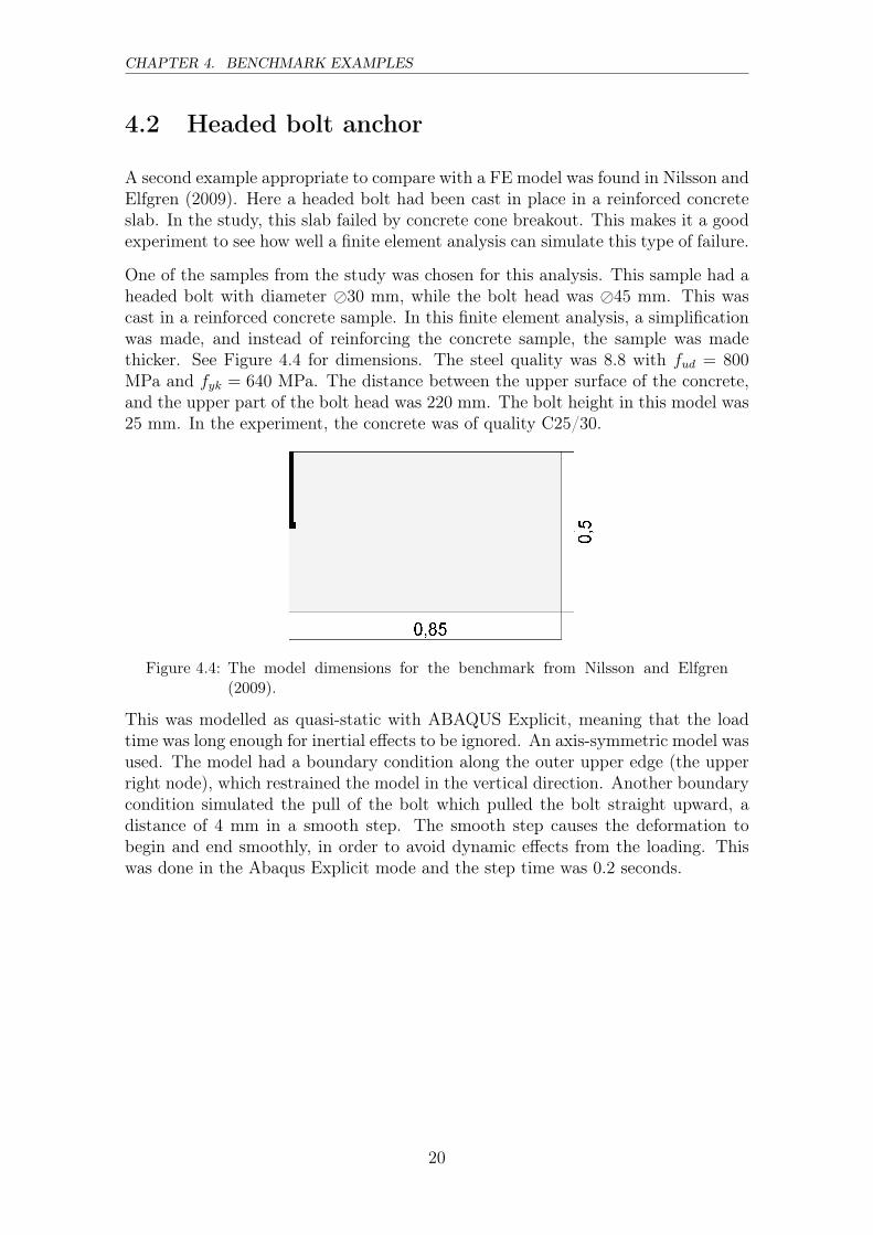
Figure 4.4: The model dimensions for the benchmark from Nilsson and Elfgren(2009).

This was modelled as quasi-static with ABAQUS Explicit, meaning that the loadtime was long enough for inertial effects to be ignored. An axis-symmetric model wasused. The model had a boundary condition along the outer upper edge (the upperright node), which restrained the model in the vertical direction. Another boundarycondition simulated the pull of the bolt which pulled the bolt straight upward, adistance of 4 mm in a smooth step. The smooth step causes the deformation tobegin and end smoothly, in order to avoid dynamic effects from the loading. Thiswas done in the Abaqus Explicit mode and the step time was 0.2 seconds.

20

4.2. HEADED BOLT ANCHOR

Figure 4.5: The meshed model

Between the bolt and the concrete, an interaction was created. The interaction prop-erties had hard conctact behaviour in the normal direction and frictionless tangentialbehaviour. This means that the bolt was prohibited from entering the concrete andthat the friction between the bolt and the concrete was not taken into account.The mesh size was 0.01, using 4-node axissymmetric reduced integration elements(CAX4R). This experiment has been previously modelled by Eriksson and Gasch(2011), but using a three-dimensional model. The concrete used for that model wasa 9 day old C25/30, which is weaker than an older concrete and has lower fractureenergy. The results they got were good and to compare, these properties has beenused in this model aswell.The steel properties come from Nilsson and Elfgren (2009).The material properties used were as follows:

Table 4.3: Concrete properties

Density 2400 kg/m3

Young’s modulus 28.4 GPaPoisson’s ratio 0.2Tensile strength 1.94 MPaCompressive strength 24.7 MPaFracture energy 48.6 Nm/m2

Table 4.4: Steel properties

Density 7800 kg/m3

Young’s modulus 200 GPaPoisson’s ratio 0.3Yield strength 640 MPaUltimate strength 800 MPa

21


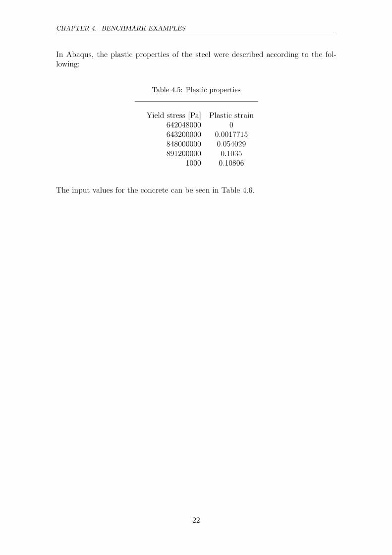
In Abaqus, the plastic properties of the steel were described according to the fol-lowing:

Table 4.5: Plastic properties

Yield stress [Pa] Plastic strain642048000 0643200000 0.0017715848000000 0.054029891200000 0.1035

1000 0.10806

The input values for the concrete can be seen in Table 4.6.

22

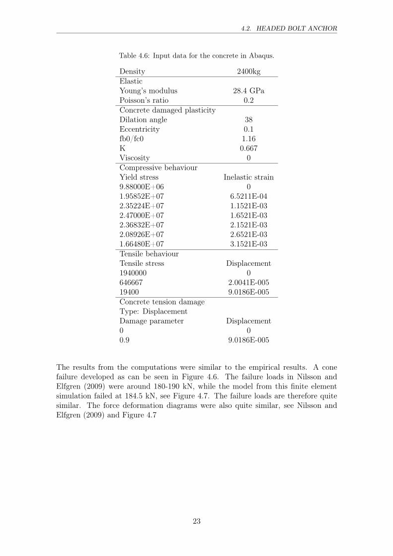
4.2. HEADED BOLT ANCHOR

Table 4.6: Input data for the concrete in Abaqus.

Density 2400kgElasticYoung’s modulus 28.4 GPaPoisson’s ratio 0.2Concrete damaged plasticityDilation angle 38Eccentricity 0.1fb0/fc0 1.16K 0.667Viscosity 0Compressive behaviourYield stress Inelastic strain9.88000E+06 01.95852E+07 6.5211E-042.35224E+07 1.1521E-032.47000E+07 1.6521E-032.36832E+07 2.1521E-032.08926E+07 2.6521E-031.66480E+07 3.1521E-03Tensile behaviourTensile stress Displacement1940000 0646667 2.0041E-00519400 9.0186E-005Concrete tension damageType: DisplacementDamage parameter Displacement0 00.9 9.0186E-005

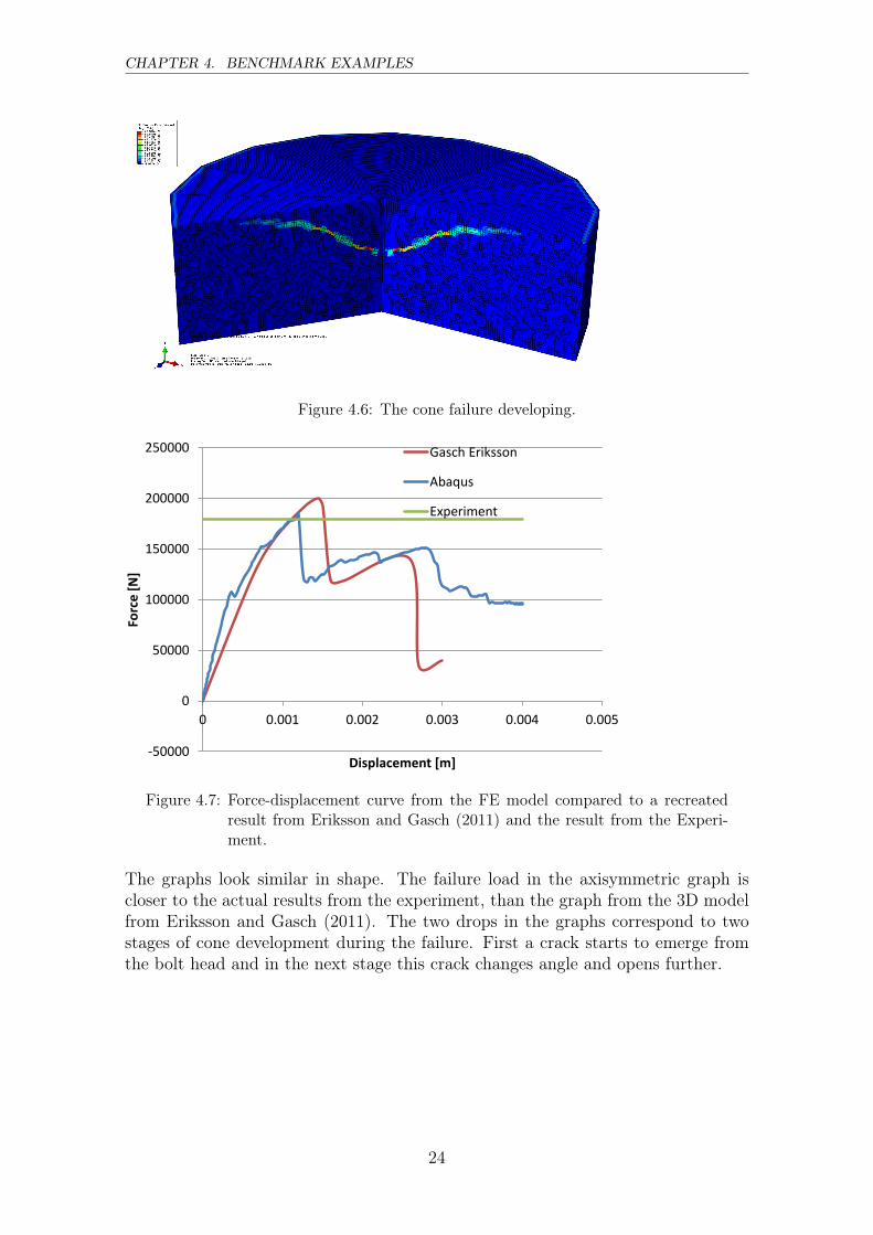
The results from the computations were similar to the empirical results. A conefailure developed as can be seen in Figure 4.6. The failure loads in Nilsson andElfgren (2009) were around 180-190 kN, while the model from this finite elementsimulation failed at 184.5 kN, see Figure 4.7. The failure loads are therefore quitesimilar. The force deformation diagrams were also quite similar, see Nilsson andElfgren (2009) and Figure 4.7

23


Figure 4.6: The cone failure developing.

-50000

0

50000

100000

150000

200000

250000

0 0.001 0.002 0.003 0.004 0.005

Forc

e [

N]

Displacement [m]

Gasch Eriksson

Abaqus

Experiment

Figure 4.7: Force-displacement curve from the FE model compared to a recreatedresult from Eriksson and Gasch (2011) and the result from the Experi-ment.

The graphs look similar in shape. The failure load in the axisymmetric graph iscloser to the actual results from the experiment, than the graph from the 3D modelfrom Eriksson and Gasch (2011). The two drops in the graphs correspond to twostages of cone development during the failure. First a crack starts to emerge fromthe bolt head and in the next stage this crack changes angle and opens further.

24

4.3. BOND FAILURE

4.3 Bond failure

The goal of the shear test was to see if a bond failure between the steel bolt and theconcrete could be correctly modelled. In this test a small axis-symmetric sample,containing only a steel bolt and a small amount of surrounding concrete was made,and boundary conditions were defined so that the failure mode would be a bondfailure. The steel bar was 0.2 meters long, and had a diameter of 25 mm. In themodel therefore the steel had a radius of 0.0125 and the concrete part was 0.025meters wide.

The connection between the steel and concrete was modelled using nonlinear springs.These were then adjusted for the mesh size when calculating the property of eachindividual spring. According to the Equation 2.2, the failure load was calculated to30.5 kN. The shear strength was here assumed to be equal to the tensile strengthof the concrete with 1.94 MPa. The material properties for concrete was definedaccording to Section 4.2. The steel properties were the same as in Table 3.2

U = F/k (4.1)

where:F: is the strength of an individual spring.U: is the deformation.k: is the spring stiffness

The mesh size for both the steel and concrete parts were 0.0125 in the horizontaldirection and 0.01176 (0.2/17) in the vertical and the elements used were again theaxisymmetric 4-node reduved integration elements (CAX4R). This made 18 springsbetween the materials, 2 of which were half strength since they were at the topand bottom. A simplification was therefore made where the values were calculatedfor 17 springs of equal strength. The value received from equation 2.2 was dividedby 17 to get the strength of each spring. A bi-linear failure-curve was then madeaccording to Section 3.1.1. The displacements were the same as in Table 4.6, butwith the elastic part of 8.0365E-07, calculated according to Equation 4.1, added tothem. The graph can be seen in Figure 4.8 and the input values were the following:

Table 4.7: Input values for the springs.

Force Displacement1.79E3 8.0365E-075.98E2 2.0845E-051.79E1 9.099E-05

25


0.00E+00

2.00E+02

4.00E+02

6.00E+02

8.00E+02

1.00E+03

1.20E+03

1.40E+03

1.60E+03

1.80E+03

2.00E+03

0.00E+00 2.00E-05 4.00E-05 6.00E-05 8.00E-05 1.00E-04

Force[N]

Deformation [m]

Figure 4.8: The spring properties.

Boundary conditions restricting movement were defined on the concrete side, seeFigure 4.9. Then a boundary condition on the top of the bolt pulled upwards ina smooth step a distance of 0.0004 meters in 0.8 seconds. This made the analysisquasi-static. Variable mass scaling scales the mass of the model and thereby reducescomputation time (Dassault Systèmes, 2014). It was used of "below min"-type andDT 5e-6 with a frequency of 100. The kinetic and internal energy-curves were closelymonitored to make sure that the mass scaling did not affect the results.

Figure 4.9: The dimensions and boundary conditions.

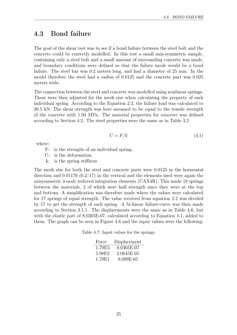
The resulting force-displacement diagram can be seen in Figure 4.10. The maxi-mum force was 32.5 kN. This differs approximately 7% from the theoretical value.However, the theoretical value does not take the deformations in the steel and con-

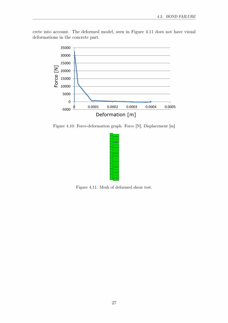
26

4.3. BOND FAILURE

crete into account. The deformed model, seen in Figure 4.11 does not have visualdeformations in the concrete part.

-5000

0

5000

10000

15000

20000

25000

30000

35000

0 0.0001 0.0002 0.0003 0.0004 0.0005

Deformation [m]

Force[N]

Figure 4.10: Force-deformation graph. Force [N], Displacement [m]

Figure 4.11: Mesh of deformed shear test.

27

Chapter 5

Load capacity of rock bolts at Limahydropower station

5.1 Field test

In 2015 the Lima hydropower station in Västerdalälven in Dalarna was recon-structed, and in the process some rock bolts were uncovered. This gave an op-portunity to test rock bolts that had been in use, but covered by concrete for 50years in order to better understand the condition of these old bolts.

Figure 5.1: The Lima Hydropower station. Photograph by Rikard Hellgren

The reconstruction process included replacing the old log chute spillway with a newspillway and spillway channel. The rock bolts used in the tests were found duringthis process. Two bolts were found just downstream of the dam body, while twoothers were found around 50 meters downstream of the dam body. The bolts inthe first group were 19 mm in diameter and placed in drill holes with 20 mm. The

29

CHAPTER 5. LOAD CAPACITY OF ROCK BOLTS AT LIMA HYDROPOWER STATION

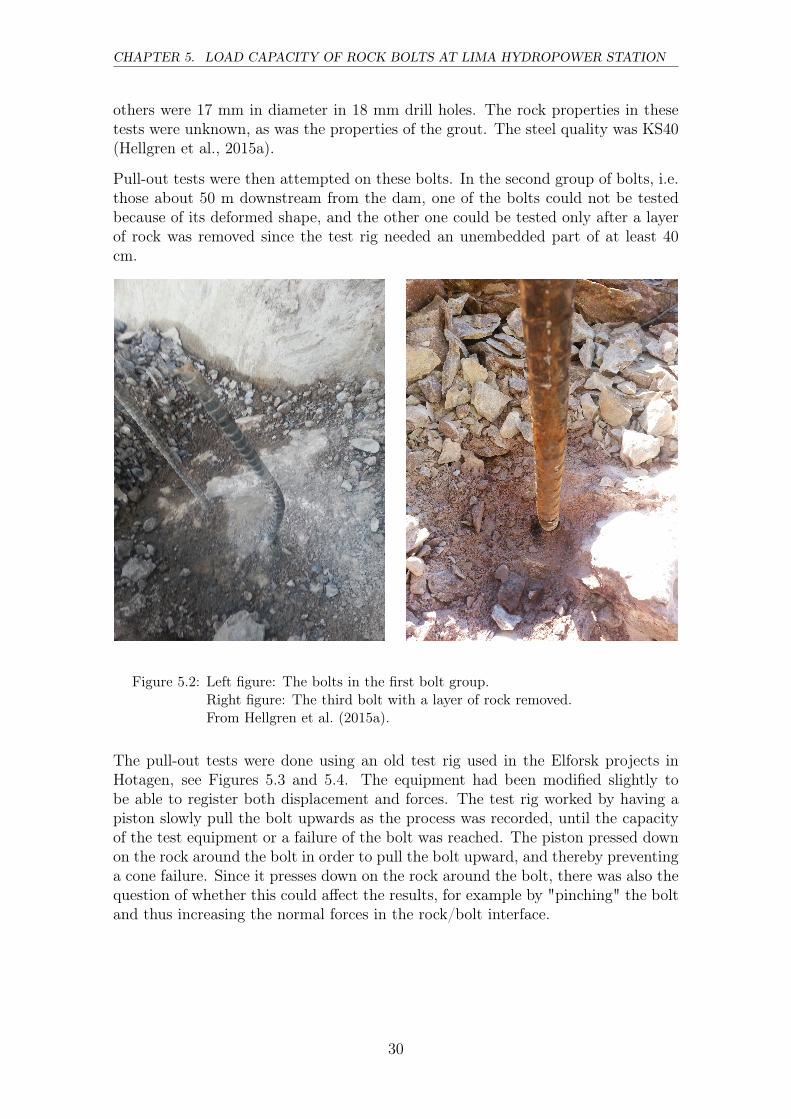
others were 17 mm in diameter in 18 mm drill holes. The rock properties in thesetests were unknown, as was the properties of the grout. The steel quality was KS40(Hellgren et al., 2015a).

Pull-out tests were then attempted on these bolts. In the second group of bolts, i.e.those about 50 m downstream from the dam, one of the bolts could not be testedbecause of its deformed shape, and the other one could be tested only after a layerof rock was removed since the test rig needed an unembedded part of at least 40cm.

Figure 5.2: Left figure: The bolts in the first bolt group.Right figure: The third bolt with a layer of rock removed.From Hellgren et al. (2015a).

The pull-out tests were done using an old test rig used in the Elforsk projects inHotagen, see Figures 5.3 and 5.4. The equipment had been modified slightly tobe able to register both displacement and forces. The test rig worked by having apiston slowly pull the bolt upwards as the process was recorded, until the capacityof the test equipment or a failure of the bolt was reached. The piston pressed downon the rock around the bolt in order to pull the bolt upward, and thereby preventinga cone failure. Since it presses down on the rock around the bolt, there was also thequestion of whether this could affect the results, for example by "pinching" the boltand thus increasing the normal forces in the rock/bolt interface.

30

5.1. FIELD TEST

Figure 5.3: The test setup used in the pullout tests at the Lima Hydropower station.Reprinted from Hellgren et al. (2015a).

Figure 5.4: The test rigg in use on the first bolt group. From Hellgren et al. (2015a).

The results from these tests can be seen in figures 5.5 and 5.6. In the graphs arealso lines indicating the yield strength of the steel of 390 MPa and the RIDAS limitof 140 MPa for this steel RIDAS (2011).

31

CHAPTER 5. LOAD CAPACITY OF ROCK BOLTS AT LIMA HYDROPOWER STATION

0 5 10 15 20 25 30 35 400

50

100

150

200

250

300

350

400

Bolt 1Bolt 2YieldRIDAS

Displacemenet [mm]

Force[kN]

Figure 5.5: The load-deformation diagram for the first two bolts in the first group.Force [kN], Deformation [mm] Recreated from Hellgren et al. (2015a).

0 5 10 15 20 25 30 350

20

40

60

80

100

120

140

Bolt 3

Yield

RIDAS

Force[kN]

Displacement [mm]

Figure 5.6: The load-deformation diagram for the bolt in the second group. Force[kN], Deformation [mm] Recreated from Hellgren et al. (2015a).

The highest measured force for bolts 1 and 2 are around 360 and 270 kN whichtranslates to around 1270 and 952 MPa. Bolt 3 reaches 140 kN or 617 MPa. Inboth of the bolt groups, these are higher than the ultimate strength of KS40 steel.

As can be seen in Figures 5.5 and 5.6, the displacements were large and no failureoccurred. At the yield stress, under the assumption that only elastic deformationshad occurred and that the Young’s modulus of the steel was 210 GPa, the displace-ment should only have been 0.7 mm. In the tests it was around 12 mm for thefirst group and 28 for the second. This leads to the idea that there has either beenslippage of the equipment on the bar, or that the rock has deformed. If the rock

32

5.1. FIELD TEST

has deformed, then there might be the possibility of the test equipment causing therock to pinch the bar, increasing the pressure and friction forces in the rock-boltinterface and changing the failure stress, or causing it to be higher than it wouldhave been without the piston pushing around the bar.

If inspecting the graphs closer, it can be seen that the graphs get stiffer in the initialpart, up until around 80 kN for the first bolt group, and 30 kN for the second boltgroup. This could be caused by some slippage of the test equipment on the bolt,and that it eventually manages to grip the bolt firmly. In the next part, the stiffnessdeclines. This can be seen especially on the third bolt. This could be caused byplasticization of the steel. In the third bolt, this happens at a force between theRIDAS guidelines and the yield stress line, while it happens after the yield stressline for the first bolt group. After this the stiffness increases again. This could bean effect of crushing of the surrounding rock.

33

Chapter 6

Numerical model of the Lima bolts

6.1 Numerical model

In order to find out if pressure around the bolt could affect the results, simulationswere made in Abaqus to see if there would be any differences in the load-deformationcurves between a model where a piston was pushing down, and one where it wasnot.For this model, initially the same concrete properties as in Section 4.2 were used.The model was made axissymmetric with a radius of 4 m and a height of 1.6 m. Thebolt has an embedded length of 1.5 meter with a radius of 0.0095 meter, as in thefirst group at Lima. The protruding part was 0.28 meters as in the sketches fromHellgren et al. (2015b). In the models with the piston, the piston was distanced0.0235 meters from the center of the bolt and had a width of 0.37 meters like thetest rig. The height was 0.4 meters. The piston had a mesh size of 0.02 m andthe bolt was around 0.1 m with axisymmetric 4-node reduced integration elements(CAX4R). The mesh size was made smaller closer to the upper left part of the model.

Figure 6.1: The model used for the calculations.

The interaction between the bolt and surrounding concrete/rock was modelled usinga friction interaction with a value of 1 according to RIDAS (2011) and interaction

35

CHAPTER 6. NUMERICAL MODEL OF THE LIMA BOLTS

properties with a hard contact in the normal direction, in order to prevent thebolt from entering the concrete, and friction in the tangential direction. Nonlinearsprings were used to simulate the shear strength as in Section 4.3, but with differentproperties in different simulations.All calculations were made using the explicit solver and with a step time of 10seconds and a mass scaling frequency of 100 with a target time increment of 5e-06.The internal and kinetic energy curves were monitored to make sure that the massscaling did not significantly affect the end result. The bottom and the right sideof the model in Figure 6.3 had boundary conditions which prohibited displacementin the horizontal and vertical directions. In the models without the pistons, adisplacement boundary condition pulled the bolt upwards a distance of 0.005 meters,and in the models with the piston, the pistons material properties caused it to expandthe same distance when exposed to heat. The pistons top was then coupled with thebolts top in the vertical direction, thus pulling the bolt upward when it expandedwhile at the same time pressing down as in the Lima-tests. The temperature riseand material properties were calculated so that the displacement would be as largeas in the other model. In both cases, the displacements were applied using smoothstep function. In the models without the piston, the reaction forces were plottedagainst the vertical displacement, and with the piston the nodal forces (NFORC)was used instead.

The embedded part of the steel was given very stiff steel properties with a Young’smodulus of 2E15 GPa. This is because the simplification of reducing an adhesivesurface into a number of springs. This will lead to the springs breaking one by one,instead of working together to reach the real failure load. This has been demon-strated in Figure 6.2 with the piston-free model from Section 6.1.3. The graph showsa very low failure load, as well as multiple bumps where the springs fail. The defor-mation is also smaller, as the springs are more brittle and the loads are too small forsignificant steel deformation. Unless otherwise stated, 16 springs were used betweenthe steel and the rock/concrete part.

36

6.1. NUMERICAL MODEL

0

5000

10000

15000

20000

25000

30000

0 0.005 0.01 0.015 0.02 0.025

Forc

e [

N]

Displacement [m]

No piston, Regular steel stiffness

Figure 6.2: The force-deformation curve when the embedded part of the steel is givenregular steel stiffness.

6.1.1 Weak grout and low strength bolt

Figure 6.3: The mesh used in this calculation.

In this model the mesh size was 0.01 m in the upper left corner of the concrete/rockand 0.1 m on the rest of the part. Since the rock properties were unknown, the sameproperties as in Section 4.2 were used for this part. The concrete had a Young’smodulus of 28.4 GPa, a tensile strength of 1.94 MPa, a compressive strength of 24.7MPa and a fracture energy of 48.6 Nm/m2. This will likely make the rock partweaker than in real life and increasing the risk of the test rig affecting the bolt. Thenonlinear springs were based on the tensile strength of that concrete type with ashear strength of 1.94 MPa and is weaker than advised in NVE (2005). The steelhad a yield strength of 370 MPa, an ultimate strength of 440 MPa and a 15 %elongation at rupture.

37


-20000

0

20000

40000

60000

80000

100000

120000

140000

160000

-0.005 0 0.005 0.01 0.015 0.02 0.025 0.03

Forc

e [

N]

Displacement [m]

No piston

Piston

Figure 6.4: Force-deformation curves of the two models.

This lead to very similar curves, with the piston-free model allowing for a slightlylarger deformation before failure. According to the formulas in Section 2.1, thisshould lead to a steel failure.

6.1.2 Higher strength grout and bolt

Here the steel was made stronger with a yield strength of 460 MPa, an ultimatestrength of 645 MPa and a 21% elongation at break. The springs were made strongerso that they would correspond to a shear strength of 2.85 MPa and the concretewas of the same type as in the previous calculation. According to the formulas, thisshould also lead to a steel failure with an even greater difference in strengths leadingto a very clear steel failure and very similar curves. While Section 6.1.1 showed asmall difference in displacement, these curves seem like an isolated steel failure.

38


-50000

0

50000

100000

150000

200000

250000

-0.005 0 0.005 0.01 0.015 0.02 0.025 0.03 0.035 0.04

Forc

e [

N]

Displacement [m]

No piston

Piston

Figure 6.5: Force-deformation curves of the two models.

6.1.3 Weak grout and stronger strength bolt

In this computaion, the shear strength has been set as 1.94 MPa, and the yieldstrength of the steel is 460 MPa. This should lead to the springs failing first witha shear failure. The concrete was the same as in the previous calculations. Sincethe springs were expected to fail, the mesh was made even smaller in the upper leftcorner with a mesh size of 0.005 meters and 0.1 in the rest of the concrete/rock partas seen in Figure 6.6.

Figure 6.6: Mesh refinement near the loading point, i.e. in the upper left corner.

The failure occured at a displacement of around 20 mm. The force-displacement

39


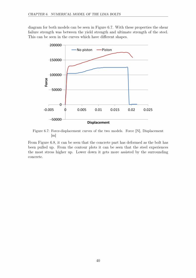
diagram for both models can be seen in Figure 6.7. With these properties the shearfailure strength was between the yield strength and ultimate strength of the steel.This can be seen in the curves which have different shapes.

-50000

0

50000

100000

150000

200000

-0.005 0 0.005 0.01 0.015 0.02 0.025

Forc

e

Displacement

No piston Piston

Figure 6.7: Force-displacement curves of the two models. Force [N], Displacement[m]

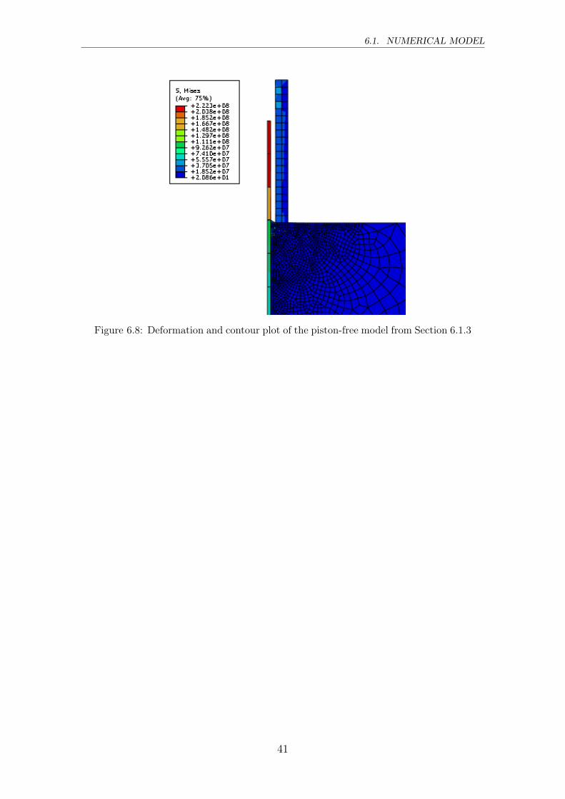
From Figure 6.8, it can be seen that the concrete part has deformed as the bolt hasbeen pulled up. From the contour plots it can be seen that the steel experiencesthe most stress higher up. Lower down it gets more assisted by the surroundingconcrete.

40


Figure 6.8: Deformation and contour plot of the piston-free model from Section 6.1.3

41

Chapter 7

Conclusions

7.1 Discussion

The objective of the thesis was to study if the test rig used for the pullout testsat the Lima hydropower station could be affecting the anchor strength of the rockbolts. To study this two models were made in Abaqus, and then compared. Onemodel where there was the effect of the test rig piston pressing down on the rockaround the bolt, and one where there was not.From the tests, a difference between the models can be seen. When the bond strengthis weaker in comparison to the steel strength, the difference grows. When the steelfailure is dominant, the curves can look very similar despite the design of the testrig. Since the steel part that is uncovered by concrete is large, there is room forlarge deformations and eventually failure in this part.

It should be noted here that the result curves with steel failure look rougher thanthey would in reality. This is because of the simplifications of the steel curve usedfor the Abaqus model. The failure curves from the analyses look like the steel curvesput into the model. This will affect the comparison of curve shapes between thesetests and the tests made at the Lima hydropower station, where the real steel curvesare rounder, and more similar to the Lima-curves than the steel curves from thesemodels. The deformations in the Lima-curves are however also larger than in theseresults. Part of this could be explained by slippage of the test rig on the bar, anddue to the difficulty of finding a flat surface for the test rig. This leads to somecrushing of the rock.

Since a failure was not obtained in the tests at Lima it is difficult to know more aboutthe properties of the grout, steel and rock, and further testing would be needed tofind these. It is therefore also difficult to try to recreate these tests more accurately.It is likely that the rock at Lima was stronger than what was used in these tests,and that the steel and shear strengths differ. For some tests in this thesis the curvesdiffered and in some cases the curves were very similar.

In conclusion, this could mean that the test rig can affect the anchor bolt strengths

43

in some cases. If the failure mode is a plasticization of the steel, then the resultdiffers little between the cases. In the case of adhesive failure however, there is asignificant effect on the result, which leads to an overestimation of the load carryingcapacity. Without further information about the different properties of the grout,steel and rock at Lima however, it can not be said to which extent it has affectedthe results in this case.

7.2 Further research

There are few articles on the subject of how to best simulate rock anchors or concreteanchors in Abaqus or other FE software. In this thesis non-linear springs wherecombined with friction-behaviour, but further studies would be needed to comparethese types of results with real pullout tests in order to find the best method orinput parameters.

There is an ongoing project that the Lima tests were a part of, where pullout tests ofold and previously embedded anchors are made. In order to get the best results fromthese tests, other test methods could be looked into. Test methods should preferablynot affect the rock close to the bolts, or hinder a rock cone failure by being too closeto the bolt. In Norway, an excavator was used in the tests (Thomas-Lepine and Lia,2014). Another example suggested in Hellgren et al. (2015b) would be to design anew tripod mounted test rig.

Bibliography

Albarwary, I. M., Haido, J., 2013. Bond strength of concrete with the reinforcementbars polluted with oil, european scientific journal, february 2013 edition vol.9,no.6.

BSK 07, 2007. Boverkets handbok om stålkonstruktioner, 4th Edition. Boverketnovember 2007.

Dassault Systèmes, 2014. Abaqus 6.14 Documentation. Providence, RI, USA.

du beton, f. f. i., 2013. fib Model Code for Concrete Structures 2010. Ernst & Sohn,Wiley.

Eligehausen, R., Mallée, R., Silva, J. F., 2013. Anchorage in concrete construction.John Wiley & Sons.

Eligehausen, R., Sawade, G., Elfgren, L., 1989. Anchorage to concrete(Chapter13).RILEM REPORT: Fracture mechanics of concrete structures - From theory toapplications (Edited by L. Elggren).

Eriksson, D., Gasch, T., 2011. Load capacity of anchorage to concrete at nuclearfacilities.

Eurocode 2: EN 1992-1-1, 2004. Design of concrete structures - Part 1-1: Generalrules and rules for buildings. Brussels.

Hellgren, Bayona, R., Malm, Johansson, 2015a. Load capacity of grouted rock bolts.

Hellgren, R., Bayona, F. R., Malm, R., Johansson, F., 2015b. Pull-out tests of50-year old rock bolts. Energiforsk-report (in preparation), ICOLD.

Hofstetter, G., Meschke, G., 2011. Numerical Modeling of Concrete Cracking.Springer Science Business Media.

Larsson, C., 2008. Utredning och provtagning av førankringsstag i Hotagens regler-ingsdamm. Elforsk rapport 09:73.

Mahrenholtz, C., Eligehausen, R., Reinhardt, H.-W., 2015. Design of post-installedreinforcing bars as end anchorage or as bonded anchor. Engineering Structures100, 645–655.

45

BIBLIOGRAPHY

Malm, R., 2009. Predicting shear type crack initiation and growth in concrete withnon-linear finite element method. Ph.D. thesis, Department of Civil and Archi-tectural Engineering, Division of Structural Design and Bridges, Royal Instituteof Technology (KTH).

Nilsson, M., Elfgren, L., 2009. Fastenings (Anchor Bolts) in Concrete Structures -Effect of Surface Reinforcement. Nordic symposium on nuclear technology, Stock-holm, 25-26 November 2009.

NVE, 2005. Retningslinjer for betongdammer. Norges vassdrags- og energidirektorat,Oslo, October 2005.

Petersson, P.-E., 1981. Crack growth and development of fracture zones in plainconcrete and similar materials. Ph.D. thesis, Division of Building materials, LTH,Lund University.

RIDAS, 2011. Swedish Hydropower companies guidelines for dam safety, applicationguideline 7.3 Concrete dams application guidelines. Svensk Energi - SwedenenergyAB.

Thomas-Lepine, C., 2012. Rock bolts - Improved design and possibilities. Master’sthesis, Department of Hydraulic and Environmental Engineering, Norwegian Uni-versity of Science and Technology.

Thomas-Lepine, C., Lia, L., 2014. Capacity of Passive Rock Bolts in Concrete DamsImproved Design Criteria. International symposium on dams in a global environ-mental challenges, Bali, Indonesia, 1-6 June, 2014.

46

TRITA 499

ISSN 1103-4297

ISRN KTH/BKN/EX-499-SE

www.kth.se

Pullout test of rock bolts at the Lima Hydropower station

Documents

Transcript of Pullout test of rock bolts at the Lima Hydropower station