Dependence of partitioning of model implicit and explicit precipitation on horizontal resolution

REVIEW ARTICLE

Dependence of partitioning of model implicitand explicit precipitation on horizontal resolution

Jorge Luıs Gomes • Sin Chan Chou

Received: 18 September 2008 / Accepted: 9 November 2009 / Published online: 3 January 2010

� Springer-Verlag 2010

Abstract Model precipitation can be produced implicitly

through convective parameterization schemes or explicitly

through cloud microphysics schemes. These two precipi-

tation production schemes control the spatial and temporal

distribution of precipitation and consequently can yield

distinct vertical profiles of heating and moistening in the

atmosphere. The partition between implicit and explicit

precipitation can be different as the model changes reso-

lutions. Within the range of mesoscale resolutions (about

20 km) and cumulus scale, hybrid solutions are suggested,

in which cumulus convection parameterization is acting

together with the explicit form of representation. In this

work, it is proposed that, as resolution increases, the con-

vective scheme should convert less condensed water into

precipitation. Part of the condensed water is made available

to the cloud microphysics scheme and another part evap-

orates. At grid sizes smaller than 3 km, the convective

scheme is still active in removing convective instability,

but precipitation is produced by cloud microphysics. The

Eta model version using KF cumulus parameterization was

applied in this study. To evaluate the quantitative precipi-

tation forecast, the Eta model with the KF scheme was used

to simulate precipitation associated with the South Atlantic

Convergence Zone (SACZ) and Cold Front (CF) events.

Integrations with increasing horizontal resolutions were

carried out for up to 5 days for the SACZ cases and up to

2 days for the CF cases. The precipitation partition showed

that most of precipitation was generated by the implicit

scheme. As the grid size decreased, the implicit precipi-

tation increased and the explicit decreased. However, as

model horizontal resolution increases, it is expected that

precipitation be represented more explicitly. In the KF

scheme, the fraction of liquid water or ice, generated by the

scheme, which is converted into rain or snow is controlled

by a parameter S1. An additional parameter was introduced

into KF scheme and the parameter acts to evaporate a

fraction of liquid water or ice left in the model grid by S1

and return moisture to the resolved scale. An F parameter

was introduced to combine the effects of S1 and S2

parameters. The F parameter gives a measure of the con-

version of cloud liquid water or ice to convective precipi-

tation. A function dependent on the horizontal resolution

was introduced into the KF scheme to influence the implicit

and explicit precipitation partition. The explicit precipita-

tion increased with model resolution. This function reduced

the positive precipitation bias at all thresholds and for the

studied weather systems. With increased horizontal reso-

lution, the maximum precipitation area was better posi-

tioned and the total precipitation became closer to

observations. Skill scores for all events at different forecast

ranges showed precipitation forecast improvement with the

inclusion of the function F.

1 Introduction

Precipitation in numerical weather prediction models may

be generated implicitly through convective parameteriza-

tion schemes and explicitly through cloud microphysics

schemes. Quantitative precipitation forecasts are particu-

larly complex for mesoscale models with resolution in the

order of tens of kilometers. At this resolution, the implicit

J. L. Gomes � S. C. Chou (&)

Center for Weather Prediction and Climate Studies (CPTEC),

National Institute for Space Research (INPE), Rod. Pres. Dutra,

km 39, Cachoeira Paulista, SP CEP 12630-000, Brazil

e-mail: [email protected]

J. L. Gomes

e-mail: [email protected]

123

Meteorol Atmos Phys (2010) 106:1–18

DOI 10.1007/s00703-009-0050-7

and explicit cloud schemes need to be used concurrently. A

realistic balance between these two schemes is a key ele-

ment for successful simulation of mesoscale convective

system (Molinari and Dudek 1992; Zhang et al. 1994;

Hong and Pan 1998). If the implicit schemes are too active,

much of the water in the atmosphere is removed by the

convective part of the scheme, while the explicit schemes

may underestimate the stratiform region and the model is

likely not to capture the internal mesoscale circulations of

such a system. On the other hand, if the implicit scheme

does not provide enough stabilization in the convective

portion of the system, the explicit schemes may overesti-

mate the grid-scale condensation and lead to exaggeratedly

intense mesoscale circulations (Zhang et al. 1988). The

activity of each of these two schemes is expected to be

greater or less, depending on the model resolution.

According to Molinari (1993), in models with grid size

greater than 20 km, the precipitation should be simulated

by implicit convective schemes with reasonable skill. In

models with grid size smaller than 3 km, which approaches

the cumulus cloud scale, the precipitation should be simulated

by explicit schemes.

Adequate partition of implicit and explicit precipita-

tion by NWP models is important for a better represen-

tation of the total precipitation and heating distribution.

With increasing resolution, the explicit scheme should

become more important and the representations of cloud

processes become more sensitive to the model grid size.

The version of the Eta Model using Kain-Fritsch

cumulus parameterization scheme tends to overestimate

precipitation over South America (Rozante and Cavalc-

ante 2008).

The objective of the present work is to evaluate the

precipitation production and partition at different hori-

zontal resolutions using the Eta Model with Kain-Fritsch

and Ferrier schemes and define a resolution-dependent

function to allow the code to self-control the precipitation

partition as resolution is changed.

This study is presented in the following manner; meth-

odology is given in Sect. 2 with a brief description of the

Eta model, the precipitation schemes and the case study;

results are discussed in Sect. 3 and conclusions are drawn

in Sect. 4.

2 Methodology

Initially, the model is run at different resolutions, and the

partition between grid-scale and subgrid-scale precipitation

is determined. Subsequently, a resolution dependency

factor is included in the model to influence the production

and partition of implicit and explicit schemes. The model is

run with different resolutions and evaluated based on

subjective and objective metrics.

The South Atlantic Convergence Zone (SACZ) case of

24–29 January 2004 was chosen for a detailed study of the

impacts of the proposed modifications included into the KF

scheme. The SACZ used in this study is described in

Sect. 2.3. The SACZ is a semi-stationary system that

accumulates large amount of precipitation over the active

period. An important feature of this system is the presence

of convective cells embedded in a region of widespread

stratiform precipitation. For additional evaluation, 4 SACZ

cases and 6 cold fronts (CF) were considered. The SACZ

cases were simulated in 132-h integrations whereas the CF

cases were simulated in 48 h.

Daily precipitation from surface rain gauges was used to

evaluate the runs. The equitable threat score (ETS) and bias

score (BIAS) are defined as in Mesinger and Black (1992)

and the model-simulated precipitation was evaluated at

points where rain gauge measurements were available.

These scores were based on 24-h precipitation

accumulations.

2.1 The Eta model

The Eta model (Mesinger et al. 1988) is a grid point model

and has a comprehensive physics package (Janjic 1990,

1994; Black 1994). It applies the eta vertical coordinate

system (Mesinger 1984). The model topography is repre-

sented as discrete steps whose tops coincide exactly with

one of the model vertical layer interfaces (Black 1994).

While the version of the Eta Model in this study was run

using the Kain-Fritsch convective scheme, the Eta model in

the United States was run using the Betts-Miller-Janjic

(BMJ) convective scheme. The model uses a semi-stag-

gered Arakawa E grid in the horizontal. The radiation

package used in the model is one developed by GFDL

(Geophysical Fluid Dynamics Laboratory). The atmo-

spheric turbulence is treated by the Mellor-Yamada Level

2.5 scheme (Mellor and Yamada 1974). The prognostic

variables are temperature, specific humidity, zonal and

meridional wind components, surface pressure, turbulent

kinetic energy and cloud hydrometeors. The lateral

boundary conditions were updated every 6 h and tendencies

were applied linearly within this time interval. The explicit

precipitation is generated by the Ferrier cloud microphysics

scheme (Ferrier 2002), hereafter referred to as FR; the

implicit precipitation by the Kain-Fritsch cumulus param-

eterization scheme (Kain and Fritsch 1990, 1993; Kain

2004), hereafter referred to as KF. Further details of the

model can be found in Black (1994) and in the Appendix B

of Pielke (2002). In the next subsection, brief descriptions

of the precipitation schemes used in the model are given.

2 J. L. Gomes, S. C. Chou

123

2.1.1 Eta model precipitation schemes

2.1.1.1 Ferrier (FR) scheme This microphysics scheme

predicts changes in water vapor and condensate in the

forms of cloud water, rain, cloud ice, and precipitation ice

(snow/graupel/sleet). The individual hydrometeors are

combined into total condensate. The water vapor and total

condensate are advected in the model.

2.1.1.2 The Kain-Fritsch (KF) scheme This scheme uses

a Lagrangian parcel method along with vertical momentum

dynamics to estimate the properties of cumulus convection.

The trigger function identifies the potential updraft source

layers associated with convection, whereas the formulation

of mass flux and the mixing rates calculates the updraft,

downdraft and the associated environmental mass fluxes.

The KF scheme rearranges mass in a column using the

updraft, downdraft, and environmental mass fluxes until at

least 90% of the convective available potential energy

(CAPE) is removed. The scheme assumes conservation of

mass, thermal energy and total moisture. In the KF scheme,

the fraction of liquid water or ice, generated by the scheme,

which is converted into rain or snow, is controlled by a

parameter S1. The S1 can be set to any value from 0, when

all condensate generated by KF scheme is converted into

convective precipitation, to 1, when all condensate is kept

as cloud water or ice and no precipitation conversion

occurs.

2.2 Proposed experiments

2.2.1 Model configuration

The Eta model was configured with 20-, 10-, and 5-km

grid sizes. For 20- and 10-km grid sizes, the vertical

resolution was set to 38 layers and the model was run in

hydrostatic mode. The time steps were 40 and 20 s,

respectively. At grid size of 5 km, the model was run in

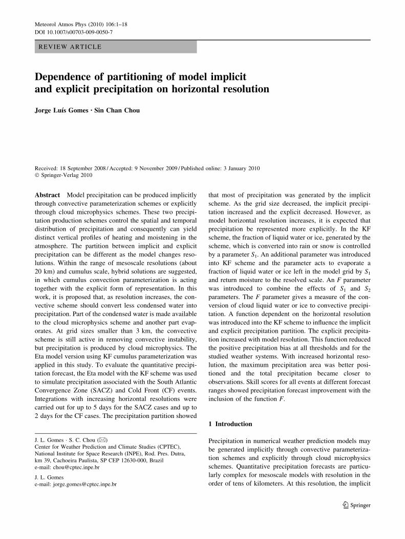
Fig. 1 Study domain in South America and topography (m). The names of the states mentioned in the text are indicated

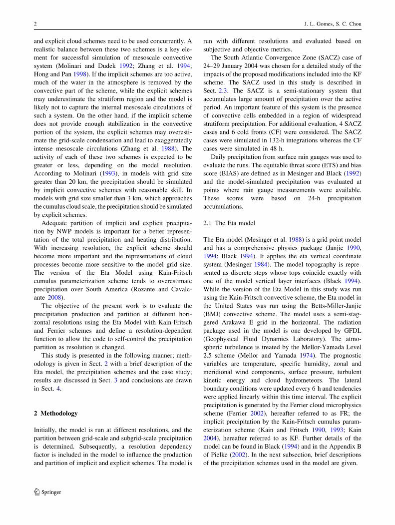
Fig. 2 Observed precipitation accumulated in period 25–29 January

2004 period (mm) for SACZ event

Dependence of partitioning of model implicit and explicit precipitation 3

123

non-hydrostatic mode with 50 layers, and the time step

was set to 10 s. The domain of the three resolutions was

set exactly the same, in order to allow comparison among

the runs. Initial and lateral boundary conditions were

taken from National Centers for Environmental Prediction

(NCEP) global analysis at T126L28 resolution. The

domain of the study is shown in Fig. 1. Major topography

feature is also shown.

2.2.2 Convective parameterization parameter tests

An additional parameter, S2, is introduced into the code and

tested. When S1 [ 0, the S2 parameter acts to evaporate a

fraction of liquid water or ice that remained in the model

grid and returns moisture to the resolved scale. In this way,

part of condensate is kept as cloud water or ice and another

part evaporates and increases environmental moisture. The

temperature and moisture tendencies due to evaporation are

applied, i.e., the environment is cooled and moistened. The

S2 can be set to any value from 0, when all cloud liquid

water or ice is kept at the model grid, to 1, when all cloud

liquid water or ice evaporates. The equations below define

the conversion of condensate generated by KF scheme into

precipitation and into cloud liquid water or ice, which is

controlled by S1. In the control version of the KF scheme,

S1 is set equal to 0. Equations 3 and 4 are introduced into

the code to express a subsequent partition of the condensate

(the cloud liquid water or ice that remained in the model

grid if S1 [ 0) which is partly kept in the model grid as

cloud liquid water or ice and partly is evaporated and

returns to model grid moisture,

CP ¼ qi 1� S1ð Þ ð1ÞCW ¼ qiS1 ð2ÞCW ¼ CW 1� S2ð Þ ð3ÞE ¼ CW� S2 ð4Þ

where CP is the convective precipitation; q is the hydrome-

teor mixing ratio (liquid water/ice); CW is the model cloud

water or ice; E is the evaporation of condensate, and S1 and S2

are the conversion and feedback parameters, respectively.

Here, the subscript i denotes the liquid water or ice.

The S1 and S2 parameters can assume any value between

0 and 1. To simplify the number of test runs, values of S1

are set equal to S2. The combined S1 and S2 values can test

the response of the model on the control of the scheme

conversion of condensate into convective precipitation. An

F parameter is introduced to combine the effects of S1 and

S2 parameters. F assumes 1 when S1 and S2 are equal to 0,

which is the case of the Control run, and physically means

that all condensate is converted into convective rain or

10N

5N

EQ

5S

10S

20S

25S

30S

35S

40S

15S

CPTECINPE

30W35W40W45W50W55W60W65W70W75W80W

296290284278272 266260254246242

(a) (b) (c)

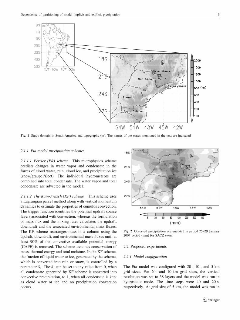
Fig. 3 (a) Infrared satellite mean brightness temperature (K) for the period between 24 and 29 January 2004; (b) streamlines and horizontal wind

divergence (shaded) (910-5 s-1) at 200 hPa; (c) streamlines and moisture convergence (shaded) at 850 hPa (910-7 g kg-1 m s-1)

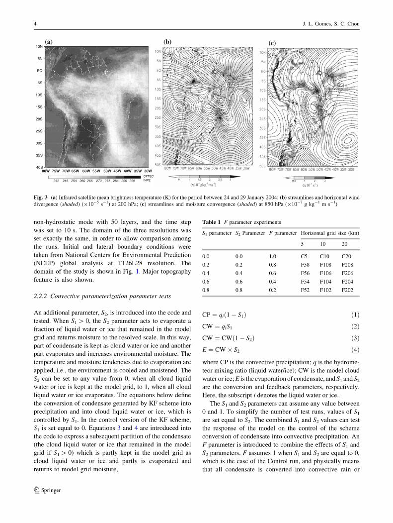
Table 1 F parameter experiments

S1 parameter S2 Parameter F parameter Horizontal grid size (km)

5 10 20

0.0 0.0 1.0 C5 C10 C20

0.2 0.2 0.8 F58 F108 F208

0.4 0.4 0.6 F56 F106 F206

0.6 0.6 0.4 F54 F104 F204

0.8 0.8 0.2 F52 F102 F202


123

snow. F assumes 0 when S1 and S2 are equal to 1, which

means that all condensate evaporates and no precipitation

is produced. The F parameter gives a measure of the

conversion of cloud liquid water or ice to convective

precipitation.

Sensitivity tests are carried out, and it is set: F = 1 - S1

and S1 = S2 = 0.8, 0.6, 0.4, 0.2, 0.0 (the latter is the

Control run).

For instance, for F = 0.8, the convective precipitation

conversion is reduced by 20%; for F = 0.6, it is decreased

by 40% and so on.

This set of experiments is carried out with model using

20-, 10-, and 5-km grid sizes. This is done in order to define

the partition of condensate to be converted into convective

rain or snow and the condensate made available to the

explicit precipitation scheme at different model grid size.

(a) (b) (c)

(d) (e) (f)

(g) (h) (i)

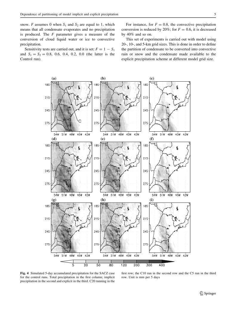
Fig. 4 Simulated 5-day accumulated precipitation for the SACZ case

for the control runs. Total precipitation in the first column; implicit

precipitation in the second and explicit in the third. C20 running in the

first row; the C10 run in the second row and the C5 run in the third

row. Unit is mm per 5 days


123

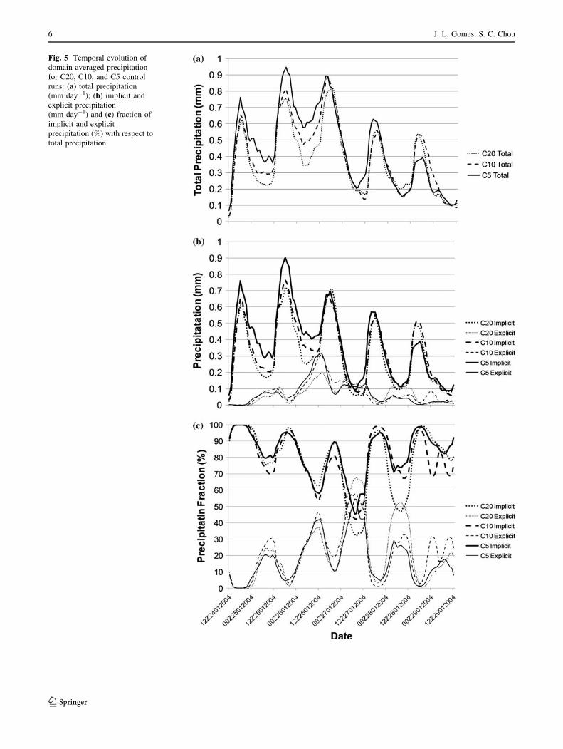
Fig. 5 Temporal evolution of

domain-averaged precipitation

for C20, C10, and C5 control

runs: (a) total precipitation

(mm day-1); (b) implicit and

explicit precipitation

(mm day-1) and (c) fraction of

implicit and explicit

precipitation (%) with respect to

total precipitation


123

2.3 Case study

The case chosen for a detailed study was the SACZ event that

established over the southeastern and southern part of Brazil

in the period 24–29 January 2004. The SACZ is an important

synoptic feature of austral summer in South America; it

shows an elongated convective band typically originating in

the Amazon basin, extending toward southeast Brazil and

into the subtropical Atlantic Ocean (Satyamurti et al. 1998;

Carvalho et al. 2002). The SACZ has been described as a

region with high variability of convective activity during

summertime in eastern South America (Liebmann et al.

1999; Zhou and Lau 1998). Carvalho et al. (2002) investi-

gated the influence of SACZ characteristics in modulating

daily extreme rainfall over Sao Paulo state, in Brazil, and they

showed that SACZ intensity and its degree of extension

toward the Atlantic Ocean determine the spatial distribution

of precipitation extremes in Sao Paulo.

In this case, the SACZ cloud band exhibited a meridi-

onal orientation and was associated with significant rainfall

over southeast Brazil, mainly in the southern part of Sao

Paulo State. It can be seen from Fig. 2, which shows the

total accumulated precipitation during the period of the

event, that the heaviest rainfall occurred in the central and

southern part of Sao Paulo where a 5-day accumulated

precipitation of 200–300 mm was observed. The precipi-

tation maxima occurred over the mountainous regions,

which indicate the role of orography in the system.

The satellite infrared image, an average taken over the

period 24–29 January 2004 (Fig. 3a), shows the presence

of the SACZ over Sao Paulo and the meridional orientation

exhibited by the cloud band, whose axis extended from

Central Brazil toward the southern part of the state of Sao

Paulo and then over the Atlantic Ocean. The cloud band

actually persisted around this position over the 5-day

SACZ period. The streamlines at upper levels show the

large-scale circulation associated with the SACZ event

(Fig. 3b). Strong divergent flow is observed in connection

with a stationary surface cold front, which established the

SACZ. The divergence extended from the Amazon basin

toward the southeastern subtropical Atlantic. The position

of the system over south and southeast Brazil was sup-

ported by an upper level trough induced by the Bolivian

High circulation and a cyclonic vortex positioned close to

the coastline of northeastern Brazil. Lower level circulation

(Fig. 3c) shows strong convergence, which transported

moisture from the Amazon basin.

3 Results

Initially, the SACZ case was run at different resolutions

with the original KF setups, and the partition of implicit

and explicit precipitation was determined at different hor-

izontal resolutions. Subsequently, the parameter F was

introduced into the KF scheme and the new partition of

implicit and explicit precipitation was evaluated. A func-

tional relationship between convective precipitation pro-

duction with horizontal resolution is proposed to the F

parameter. Table 1 lists the parameter values and the

experiments’ names.

3.1 Resolution tests

The model was run with the original KF to evaluate the

dependence of the implicit and explicit precipitation par-

tition in the Eta Model on horizontal resolution. It is

expected that as horizontal resolution increases, the explicit

scheme should be more important because the model

resolvable scale becomes cloud scale, and in this case the

activity of the implicit scheme should diminish and the

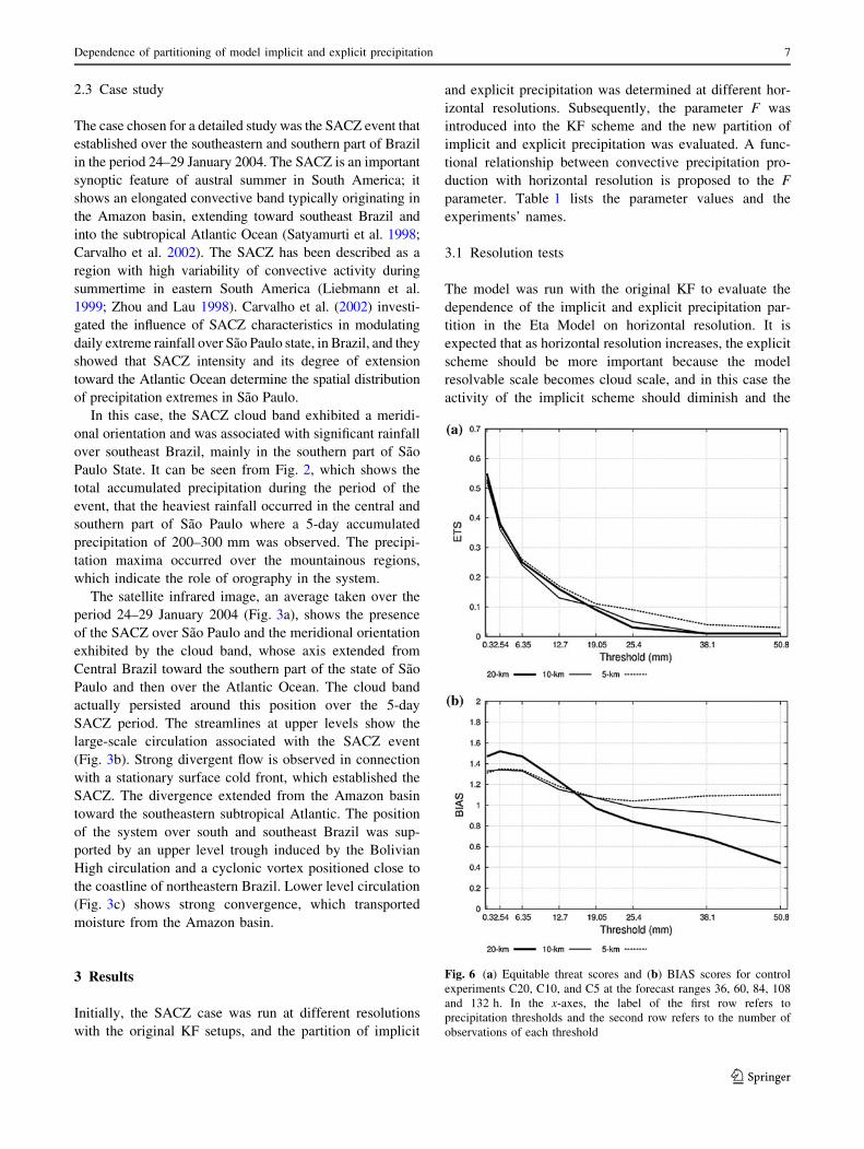
Fig. 6 (a) Equitable threat scores and (b) BIAS scores for control

experiments C20, C10, and C5 at the forecast ranges 36, 60, 84, 108

and 132 h. In the x-axes, the label of the first row refers to

precipitation thresholds and the second row refers to the number of

observations of each threshold


123

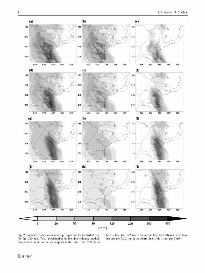
Fig. 7 Simulated 5-day accumulated precipitation for the SACZ case

for the C20 run. Total precipitation in the first column; implicit

precipitation in the second and explicit in the third. The F208 run in

the first line; the F206 run in the second line; the F204 run in the third

line and the F202 run in the fourth line. Unit is mm per 5 days


123

explicit scheme should treat not only the cumulus con-

vective cloud, but also the stratiform clouds. The control

runs are labeled as C20, C10, and C5 for 20-, 10- and 5-km

grid sizes, respectively.

The simulated total precipitation for the C20 (Fig. 4a)

shows that the position of the system was displaced to the

south as compared to observations (Fig. 2). The CD line in

Fig. 4a shows the position and orientation of the maximum

precipitation activity of the SACZ and the AB line refers to

the position of the simulated precipitation band. Thus, the

observations showed that the simulated precipitation band

was displaced to the south. In this case, the maximum

5-day accumulated precipitation was 400 mm over Santa

Catarina State, whereas in the observations the amounts

were smaller and positioned over Sao Paulo State.

The implicit and explicit precipitation amounts (Fig. 4b,

c) show that most of precipitation was generated by the

implicit scheme at the 20-km grid size. At this resolution, it

was found that the explicit scheme missed the SACZ

stratiform region (Fig. 4c), this was represented by the

convective scheme. The explicit scheme acted over the

region of maximum precipitation core. It expected that the

explicit scheme should generate the widespread precipita-

tion and the implicit scheme should generate the intense

and localized precipitation at lower resolution. However, as

grid size was reduced to 10 km, the total precipitation

simulated by the C10 experiment (Fig. 4d) showed that the

spatial distribution was almost the same as for the C20. The

region of the precipitation core expanded, especially over

Parana state and most of Santa Catarina state, and the core

of maximum precipitation increased in magnitude. In

addition, the implicit scheme generated the larger part of

the total precipitation. The explicit precipitation (Fig. 4f)

showed a small increase in the amount and areal extension,

but as in the C20 run, the explicit scheme missed the

stratiform precipitation region. The areas where the explicit

precipitation intensified were associated with the areas

where the implicit precipitation also intensified.

As the grid size changed to 5 km, the total precipitation

(Fig. 4g) showed a small contraction in the precipitating

area and an increase in the simulated maximum values. As

in the C20 and C10 runs, the implicit scheme from the C5

run produced most of the total precipitation. A contraction

in area and an intensification of the precipitation maxima

can be noticed for the implicit precipitation. The same

pattern of contraction and intensification of precipitation

with increasing resolution was found in the explicit pre-

cipitation, suggesting that the implicit scheme modulates

the location where the explicit scheme acts.

As grid size reduced from 20 to 5 km (Fig. 4a, d, g), the

position of the simulated SACZ band did not improve, i.e.,

it was displaced to the south when compared against

observations (Fig. 2). It can be noticed that the implicit

scheme acted strongly, with the localized 5-day accumu-

lated maxima between 300 and 400 mm for the C20 run

and up to 500 mm for the C5 run. With the resolution

increase, comparisons of the C20 versus C10 and C10

versus C5 runs show the displacement of the precipitation

band toward the north and also show an increase in the

localized total precipitation maxima (figures not shown).

Figure 5a shows the simulated total precipitation aver-

aged over the model domain during the integration period.

The minima and maxima are produced at about the same

time for each resolution (Fig. 5). In the 5-day accumulated

precipitation, it was found an increase of total precipitation

of about 8% for C10 run with respect to the C20 run, and

an increase of about 20% for C5 run. The implicit and

explicit precipitation each increased by 8 and 11%,

respectively, for the C10, and 22 and 8% for C5 runs with

respect to C20 run. This model behavior is opposite to what

is expected as horizontal resolution increases, for most of

the explicit precipitation should increase as model grid size

decreases. However, in this case, the implicit precipitation

increased and the explicit precipitation decreased with

decrease of the grid size from C10 to C5. Figure 5b shows

the temporal evolution of domain-averaged implicit and

explicit precipitation, in comparison with total precipita-

tion. It shows that implicitly represented precipitation

contributed most of the total precipitation even at higher

resolution. The explicit and implicit precipitation curves

are out of phase. When the implicit curve is at its peak, the

explicit is at its minimum, and the other way round. In

addition, the explicit precipitation is always smaller than

Table 2 Percentage of change of total, implicit and explicit precip-

itation from 20-, 10-, and 5-km grid sizes runs with respect to the

control runs C20, C10, and C5, respectively, averaged over whole

domain and over SACZ period

Runs Total (%) Implicit (%) Explicit (%)

20 km

F208 -6 -11 18

F206 -13 -30 61

F204 -23 -53 113

F202 -28 -76 189

10 km

F108 -1 -6 26

F106 -9 -25 62

F104 -23 -51 102

F102 -31 -75 167

5 km

F58 13 7 38

F56 4 -14 81

F54 -10 -42 102

F52 -21 -70 202


123

the implicit even at higher resolution. The fraction of

explicit precipitation with respect to total precipitation is

still below 50% (Fig. 5c), even when the implicit precipi-

tation fraction is at its minimum.

The equitable threat scores (ETS) of 24-h accumulated

precipitation forecast (Fig. 6a) show almost the same skill

at low precipitation rates for the C20, C10 and C5 runs. At

rain rates higher than 19.05 mm day-1, the higher resolu-

tion run has the best skill, while C10 and C20 have similar

skill. The corresponding bias scores (Fig. 6b) show that at

smaller grid sizes (5- and 10-km) rain is overestimated at

all thresholds, whereas at lower resolution, heavy precipi-

tation is underestimated.

The precipitation bias increased at higher thresholds,

38.1 and 50.8 mm, as horizontal resolution increased

(Fig. 6b). The improvement of the 5-km ETS was

accompanied by an overestimate of total precipitation. The

time evolution of the sea level pressure showed that the

center of low pressure associated with the system was

deeper when compared with the analysis and displaced to

the southeast. By decreasing the grid size, the center was

deeper (Figures not shown).

These model version runs failed to represent accurately

the SACZ rain band position. The evaluation of the runs

showed that the increase of horizontal resolution had only a

slight improvement in model performance. In addition, the

partition between explicit and implicit rain does not seem

correct.

3.1.1 Precipitation partition

The simulated precipitation for a set of F parameter values

of the 20-km grid size experiments can be seen in Fig. 7.

The total precipitation for the SACZ period is shown in the

first column, the implicit and explicit precipitation in the

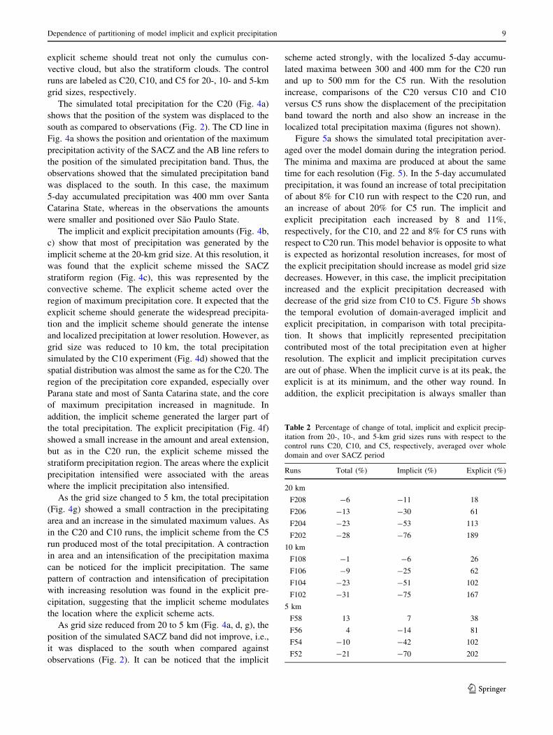
Fig. 8 Temporal evolution of domain-averaged precipitation

(mm day-1) for 20-km F parameter runs: (a) total precipitation, (b)

implicit precipitation, and (c) explicit precipitation. Solid lines refer

to F208 run; dash-dot, F20; dashed, F204; and dotted, F202

(a)

(b)

Fig. 9 (a) Equitable threat scores and (b) bias scores for experiments

F208, F206, F204, and F202 at the forecast ranges 36, 60, 84, 108,

132 h. In the x-axes, the label of the first row refers to precipitation

thresholds and the second row refers to the number of observations of

each threshold


123

second and third columns, respectively. In the F208

experiment, when the F was reduced to 0.8, the total

simulated precipitation (Fig. 7a) shows a slight reduction

and small change in position of the SACZ band toward the

east when compared with the control run (Fig. 4a). It is

noted that this change in total precipitation was caused by

the reduction of the implicit precipitation. As less liquid

water was converted to precipitation, the implicit precipi-

tation decreased and the explicit precipitation increased.

The greater availability of liquid water for the explicit

scheme contributed to an increase in the amount and area

of precipitation produced by the explicit scheme (Fig. 7c, f,

i). Table 2 shows the percentage change of total, implicit

and explicit precipitation from these runs with respect to

the C20, C10 and C5 runs, averaged over whole domain

and period of the SACZ event. A decrease of implicit

precipitation can be seen in the F206, F204, and F202 runs

and, consequently, the explicit scheme became more active

and the precipitation produced by this scheme was larger.

A decrease in implicit precipitation of about 13, 23, and

28% caused an increase of about 61, 113, and 189% in the

explicit precipitation in the F206, F204, and F202 runs,

respectively. However, the total precipitation did not

increase with resolution. The implicit precipitation reduced

the amount of precipitation by about 13, 23, and 28%. It

was noted that the increase of explicit scheme activity

contributed to position the precipitation maximum further

to the north (Fig. 7a, d, g, j). The position of the system

simulated by all F experiments was better than the control

runs. Note that the F experiments produced different

distributions and amounts of implicit and explicit precipi-

tation. In spite of better position of the SACZ, all F runs

failed to represent the stratiform precipitation area.

Similar behavior was noted in the spatial distribution of

precipitation for the 10- and 5-km grid sizes to that found

at 20-km grid size, in which the implicit precipitation

decreases as F decreases (figures not shown). The explicit

scheme showed an increase in the precipitation amount and

contributed to a better representation of the position of the

SACZ. Despite the change in the horizontal resolution, the

changes of total, implicit and explicit precipitation were

almost the same.

Figure 8 shows the time evolution of the precipitation at

20-km grid size—total, implicit and explicit—averaged

over the model domain, for the set of F parameters. The

decrease of the F parameter reduces the total precipitation.

The change in the phase of the time of occurrence of the

peak of maximum implicit precipitation with respect to

explicit precipitation for run F202 can also be noted. The time

evolution of the implicit precipitation (Fig. 8) shows that with

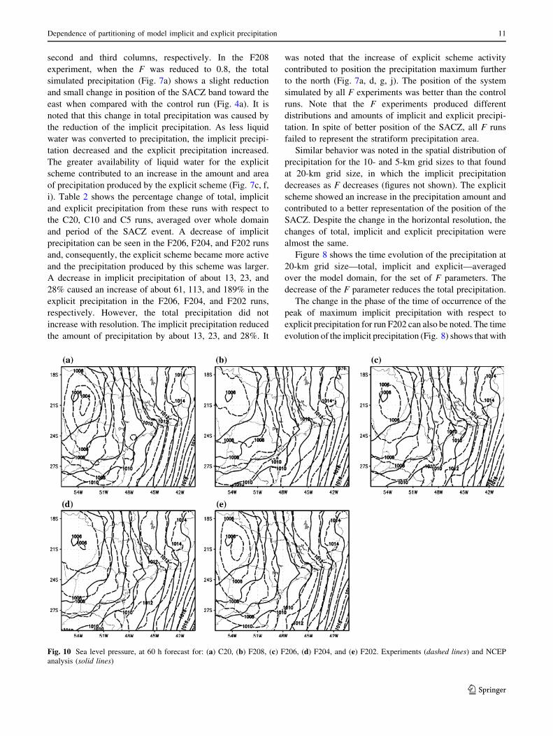
Fig. 10 Sea level pressure, at 60 h forecast for: (a) C20, (b) F208, (c) F206, (d) F204, and (e) F202. Experiments (dashed lines) and NCEP

analysis (solid lines)


123

the reduction of the F there is a gradual decrease of the total

precipitation generated by the KF convection scheme.

The opposite is seen for the explicit precipitation

(Fig. 8c), where the reduction of F brought some increase in

the amount of precipitation generated by the FR cloud

microphysics scheme. In both types of precipitation, there

are no changes in the timing of maxima and minima. With

the increase in availability of moisture at a model grid point

due to the reduction of F, the explicit scheme can be more

active, thus generating more precipitation that is explicit.

The maximum activity of the explicit scheme occurs at

the time of minimum activity of the implicit scheme, as

seen in the control run C20. The increase in the activity of

the explicit scheme contributes toward delaying the max-

ima of total precipitation (Fig. 8a). In these cases, the

larger portion of the total precipitation is due to the explicit

scheme. This pattern becomes clear in run F202, where the

reduction in the F is larger and consequently, there is

greater activity in the explicit scheme.

The same patterns of evolution of total, implicit and

explicit precipitation described above were found in the

experiments with the parameter F at grid sizes of 10 and 5 km,

where the implicit scheme simulated less precipitation. Con-

sequently, the explicit scheme became more active, thus

generating a larger amount of explicit precipitation (figure not

shown). As in the case of 20-km grid size, the experiments

with variation in F at 10 and 5 km indicated a better posi-

tioning of the SACZ. This improvement was due to the

increase in explicit precipitation simulated by the model.

3.1.2 Precipitation evaluation

The ETS for a set of F experiments at 20-km grid size (Fig. 9a)

shows an increase of the skill as F decreases. The reduction of

F to 0.8 in the F208 run results in a small increase in the model

skill when compared with C20 run. For further F decreases,

i.e., by 0.6, 0.4 and 0.2 for F206, F204 and F202, respectively,

a gradual increase was observed in the model precipitation

skill. In comparison with the C20 runs, the improvements

were considerable for all thresholds, especially above

19.05 mm. For the corresponding BIAS scores (Fig. 9b),

when the F was reduced, a gradual reduction was noted for the

lower and medium thresholds. For higher thresholds, the

BIAS was close for all F experiments. These reductions were

due to the reduction of the implicit precipitation production

influenced by the change of the F parameter from 1 (control

run) to 0.2 (F202). Those runs resulted in better ETS than the

C20 run. Similar scores were found at the 10- and 5-km grid

sizes (figures not shown). The improvement of ETS as F

decreases for the three resolution runs was due to better

positioning of the system, in all F experiments. Therefore, it

was noticed that changes of F value have larger impact on

precipitation than horizontal resolution.

3.1.3 F parameter effects

In order to relate the mechanisms that produced the posi-

tive impacts with the inclusion of F parameter, an exami-

nation of scheme effects is included for the 20-km

experiments.

Figure 10 shows the mean sea level pressure, at 60-h

forecast for C20, F208, F206, F204 and F202 experiments

runs (dashed lines) and NCEP analysis (solid lines). As the

F of the KF scheme was reduced, the sea level pressure was

better simulated. The improvement was observed for

reduction of F up to 0.4 (Fig. 10b–d). When the F was

equal to 0.2, the center of low pressure was deeper. The

same pattern was observed in the 10-km experiments

(figures not shown). For 5-km experiments, the pattern of

Fig. 11 (a) Difference between cloud liquid water and ice produced

by the F206 experiment and the C20 Control run at 500-hPa (g kg-1);

(b) Mean wind (vector) and difference of the zonal wind component

between the F206 experiment and C20 Control run (shaded) (m s-1).

Means were taken in the period between 25 January 2004, 12Z and 27

January 2004, 12Z


123

sea level pressure improved when F was changed to 0.6

(figures not shown). In the upper level, the trough associ-

ated with the surface cold front shifted to the east as F was

decreased and the divergent flow moved toward north.

These results are consistent with the displacement of the

surface cold front toward north. This pattern was observed

for all model grid sizes tested (20-, 10-, and 5-km). The

comparison of the upper air circulation against the NCEP

analysis indicates that the F206, F104, and F54 runs do the

better simulations (figures not shown).

Figure 11a shows the difference between the 500-hPa

cloud liquid water and ice produced by the F206 experi-

ment and the C20 Control run. This is the mean difference

taken in the period between 25 January 2004, 12Z and 27

January 2004, 12Z, when precipitation within the SACZ

band was more active. Positive values show the increase of

cloud liquid water and ice produced by the modified

scheme to the east of the Control C20 rain band and

therefore approaching the position of the observed pre-

cipitation area.

Figure 11b shows the 500-hPa wind vector and the

zonal wind component difference between the F206

experiment and C20 Control run. These are average values

over the same period as Fig. 11a. The positive differences

of zonal wind show the increase of zonal wind speed in the

region where cloud liquid water and ice were added by the

F206 experiment; this combination yields an eastward

advection of the cloud and subsequent increased precipi-

tation to the east of the C20 Control run.

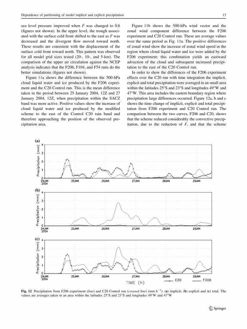
In order to show the differences of the F206 experiment

effects over the C20 run with time integration the implicit,

explicit and total precipitation were averaged in an small area

within the latitudes 25�S and 23�S and longitudes 49�W and

47�W. This area includes the eastern boundary region where

precipitation large differences occurred. Figure 12a, b and c

shows the time change of implicit, explicit and total precipi-

tation from F206 experiment and C20 Control run. The

comparison between the two curves, F206 and C20, shows

that the scheme reduced considerably the convective precip-

itation, due to the reduction of F, and that the scheme

Fig. 12 Precipitation from F206 experiment (line) and C20 Control run (crossed line) (mm h-1): (a) implicit; (b) explicit and (c) total. The

values are averages taken in an area within the latitudes 25�S and 23�S and longitudes 49�W and 47�W


123

increased significantly the explicit precipitation. A delay in

the peaks of implicit precipitation can be noticed in the F206

experiment. In this experiment, the explicit precipitation was

an important contribution to the total precipitation during the

most active SACZ period, between 25 January 2004 12Z and

27 January 2004 12Z. The experiment showed the change in

the partition between implicit and explicit precipitation in the

small defined area.

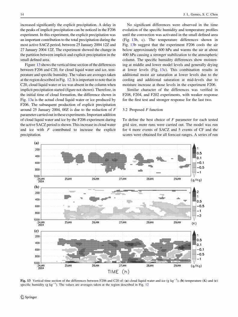
Figure 13 shows the vertical time section of the differences

between F206 and C20, for cloud liquid water and ice, tem-

perature and specific humidity. The values are averages taken

at the region described in Fig. 12. It is important to note that in

C20, cloud liquid water or ice was absent in the column when

implicit precipitation started (figure not shown). Therefore, in

the initial time of cloud formation, the difference shown in

Fig. 13a is the actual cloud liquid water or ice produced by

F206. The subsequent production of explicit precipitation

around 25 January 2004, 00Z is due to the reduction of F

parameter carried out in these experiments. Important addition

of cloud liquid water and ice by the F206 experiment during

the active SACZ period is shown. This increase in cloud water

and ice with F contributed to increase the explicit

precipitation.

No significant differences were observed in the time

evolution of the specific humidity and temperature profiles

until the convection was activated in the small defined area

(Fig. 13b, c). The temperature differences shown in

Fig. 13b suggest that the experiment F206 cools the air

below approximately 600 hPa and warms the air at about

400 hPa causing a stronger stabilization to the atmospheric

column. The specific humidity differences show moisten-

ing at middle and lower model levels and generally drying

at lower levels (Fig. 13c). This combination results in

additional moist air saturation at lower levels due to the

cooling and additional saturation at mid-levels due to

moisture increase at those levels in the experiment F206.

Similar character of the differences was verified in

F208, F204, and F202 experiments, with weaker response

for the first test and stronger response for the last two.

3.2 Proposed F function

To define the best choice of F parameter for each tested

grid size, more runs were carried out. The model was run

for 4 more events of SACZ and 5 events of CF and the

scores were obtained for all forecast ranges. A series of run

Fig. 13 Vertical time section of the differences between F206 and C20 of: (a) cloud liquid water and ice (g kg-1); (b) temperature (K) and (c)

specific humidity (g kg-1). The values are averages taken at the region described in Fig. 12


123

were carried out, each event was run with F parameter

equal to 0.8, 0.6, 0.4, and 0.2. The best F for each reso-

lution was chosen, and their scores were shown in Fig. 14.

The chosen F parameter runs show higher precipitation

ETS than the control runs. This improvement is clearer in

the 5-km runs. Positive biases are present in the KF runs,

particularly for 10- and 5-km grid sizes, where bias is

approximately constant in most of thresholds. The modi-

fication included into the KF changed the behavior of the

BIAS score to one single pattern for the three resolutions:

overestimation at smaller thresholds and underestimation at

higher thresholds. This seems that the precipitation bias is

no longer strongly dependent on horizontal resolution, but

the remaining biases may be, as hypothesis, mostly due to

physics of the model.

The set of runs carried out suggested that for 20-km

grid size the value of the F should be approximately 0.6

and for 10- and 5-km should be approximately 0.4. A

resolution-dependent function for F is proposed and

included into the KF scheme code; thus, given the size of

grid, the adjustment of the partition of the implicit and

explicit precipitation will be controlled by the following

function of F:

FðDxÞ ¼

0; Dx� 3 km

0:4; 3 km\Dx� 10 km

0:02� Dxþ 0:2; 10 km\Dx\40 km

1; Dx� 40 km

8>><

>>:

ð5Þ

where Dx is the model grid size in km.

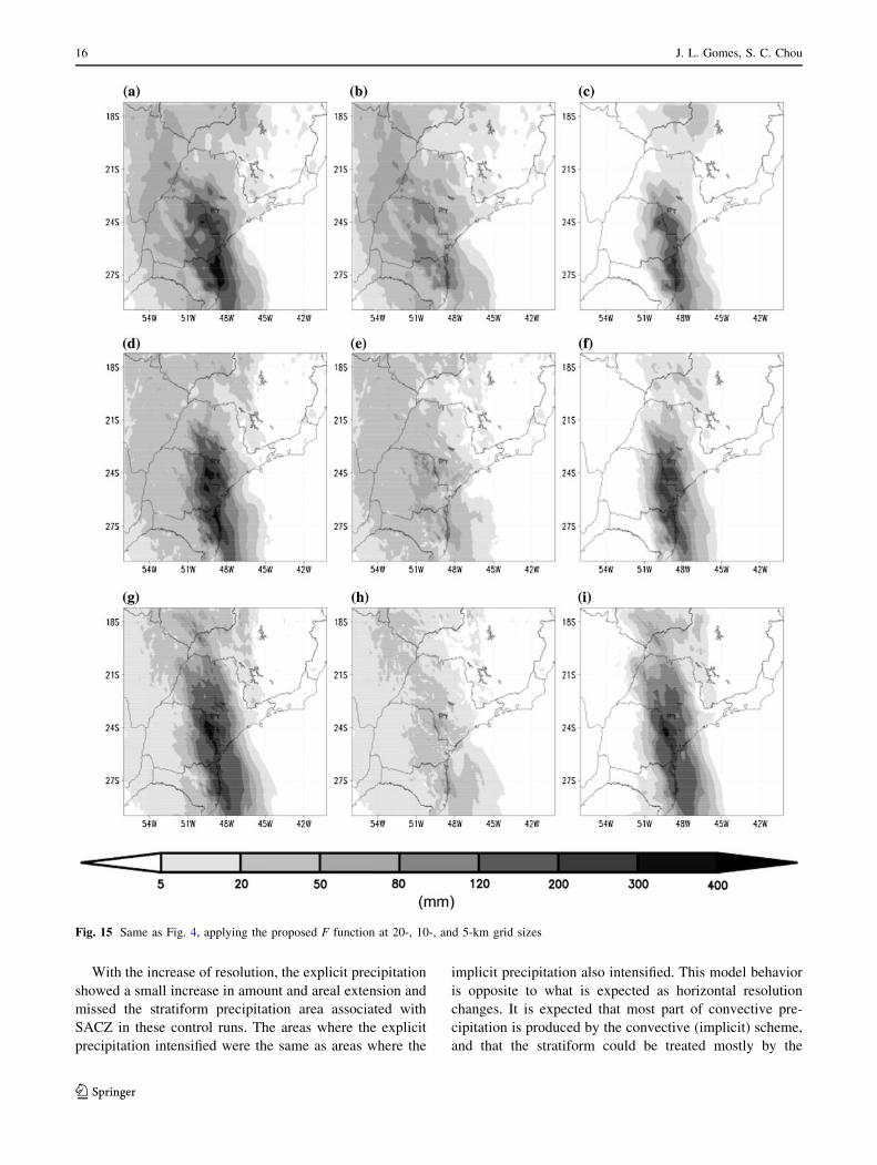
Figure 15 shows the results of the inclusion in the

model of the proposed generalized partition of the pre-

cipitation given by (5). The model was re-run for the case

study of Sect. 2.3 at the 20-, 10-, and 5-km grid sizes, as

in Fig. 4, the total, implicit, and explicit precipitation

were accumulated over the 5 days of the SACZ event.

The first, second, and third columns indicate, respectively

the total, implicit, and explicit precipitation. As the grid

size decreased from 20 to 10 km, the implicit scheme

became less active and produced less precipitation, while

the explicit scheme became more active, and produced

more precipitation. When the grid size decreased from 10

to 5 km, the implicit scheme produced slightly more

precipitation and the explicit scheme reduced the amount

of maximum precipitation. On the other hand, in com-

parison with the control run C05, higher resolution, the

function-modified KF run decreased the implicit and

increased the explicit precipitation, as was sought

initially.

4 Summary and conclusion

Control runs carried out with the Eta Model at 20-, 10-, and

5-km grid sizes with the original implicit and explicit

precipitation schemes showed that the model overestimated

precipitation, mainly at higher resolution, and had some

positioning error in the precipitation band associated with

the SACZ event. These runs displaced the precipitation

associated with the SACZ band to the south as compared to

observations. The maximum 5-day accumulated simulated

precipitation was over SACZ region, whereas in the

observations the amounts were smaller and positioned to

the north over Sao Paulo State. As resolution increased, the

maximum SACZ core intensified and expanded the band.

The position of the rain band was almost at the same place

for all resolutions in the control runs. The implicit scheme

produced the largest contribution to the total precipitation

in the control runs.

Fig. 14 (a) Equitable threat scores; (b) BIAS scores, for all forecast

ranges (36, 60, 84, 108, 132 h), for 10 precipitation cases. Control

runs are indicated by thin lines and F parameter runs indicated by

thick lines. In the x-axes, the label of the first row refers to

precipitation thresholds and the second row refers to the number of

observations of each threshold


123

With the increase of resolution, the explicit precipitation

showed a small increase in amount and areal extension and

missed the stratiform precipitation area associated with

SACZ in these control runs. The areas where the explicit

precipitation intensified were the same as areas where the

implicit precipitation also intensified. This model behavior

is opposite to what is expected as horizontal resolution

changes. It is expected that most part of convective pre-

cipitation is produced by the convective (implicit) scheme,

and that the stratiform could be treated mostly by the

Fig. 15 Same as Fig. 4, applying the proposed F function at 20-, 10-, and 5-km grid sizes


123

explicit scheme, and as resolution increases, the convective

scheme should give less contribution and the explicit

scheme should account for both stratiform and convective

precipitation.

The temporal evolution of mean precipitation in the

control run shows that the implicit precipitation produced

the larger fraction of total precipitation during the whole

integration period. It is noted that the explicit scheme is

allowed to be more active when the implicit scheme is less

active.

The verification demonstrated that the control runs at

different resolutions had similar ETS for all precipitation

thresholds. A small improvement was found in the C5 run,

at the expense of overestimating the amount and areal

coverage of the precipitation.

The version of the Eta Model using Kain-Fritsch

cumulus parameterization scheme tends to overestimate

precipitation over South America. In order to affect the

partition of the total precipitation between explicit and

implicit, with resolution changes, a set of parameter F was

tested with different grid sizes. The F parameter varied

from 0.2 to 0.8. The F parameter influenced the implicit

and explicit precipitation partition. As F decreases, less

liquid water is converted as convective rain and, conse-

quently, more water is made available to other schemes,

particularly to the cloud microphysics scheme. In addition,

with a more realistic balance between the implicit and

explicit schemes, the model could be able to capture the

internal mesoscale circulations associated with the system

and produced better simulations. The simulation of the

SACZ event showed that the diurnal cycle of the grid-scale

(implicit) and subgrid-scale (explicit) was changed and the

location of the precipitation bands was altered and better

agreed with the observations. In surface, the model simu-

lation of mean sea level pressure was better represented

when the F was reduced to 0.6 for 20-km grid size and to

0.4 for 10- and 5-km grid sizes. In the upper level, the

trough associated with the surface cold front shifted to the

east as F was decreased and the divergent flow moved

toward north.

The variation of the F parameter had a larger impact in

the precipitation scores of the SACZ event chosen for a

detailed study. This new precipitation partitioning reduced

the overestimate found in the control runs. The improve-

ment of ETS as convective precipitation decreased for the

three resolution runs was due to better positioning of the

system, in all F experiments. Changes of F value showed

larger impact on precipitation than horizontal resolution.

More cases were added to the evaluation and the impact of

the introduction of the F parameter into the KF scheme was

positive. The experiments with different F parameters

showed either marginal or clear improvement, but no

degradation.

A generalized F function dependent on grid size is pro-

posed. This function reduced the original positive precipitation

bias at all thresholds and for the studied weather systems. With

increased horizontal resolution, the maximum precipitation

area was better positioned and the total precipitation became

closer to observations. Skill scores for all events at different

forecast range showed precipitation forecast improvement

with the inclusion of the function These results show that the

increase of resolution in general requires additional model

tuning and verification, as some previous scale assumptions in

the design of the schemes may have broken down.

In a future phase of this work, adjustments will be made

in the explicit precipitation scheme to augment its activity

and reduce the negative bias found mainly in the areas of

intense precipitation.

Acknowledgments The authors would like to thank the reviewers

for their useful comments which helped to improve the manuscript.

This work is a contribution to the Serra do Mar Project, partly funded

by FAPESP under grant no. 04/09649-0 and partly funded by CNPq

under grant no. 308725/2007-7.

References

Black TL (1994) The new NMC mesoscale Eta model: description ad

forecast examples. Weather Forecast 9:265–278

Carvalho LMV, Jones C, Liebmann B (2002) Extreme precipitation

events in Southeastern South America and large-scale convective

patterns in the South Atlantic convergence zone. J Clim

15:2377–2394

Ferrier BS, Lin Y, Black T, Rogers E, DiMego G (2002) Implemen-

tation of a new grid-scale cloud and precipitation scheme in the

NCEP Eta model. In: 15th Conference on numerical weather

prediction, American Meteorological Society, San Antonio, TX,

pp 280–283 (preprint)

Hong S-Y, Pan H-L (1998) Convective trigger function for a mass-flux

cumulus parameterization. Mon Weather Rev 126:2599–2620

Janjic ZI (1990) The step-mountain eta coordinate: physical package.

Mon Weather Rev 118:1429–1443

Janjic ZI (1994) The step-mountain coordinate model: further

developments of the convection, viscous sublayer, and turbu-

lence closure schemes. Mon Weather Rev 122:927–945

Kain JS (2004) The Kain-Fritsch convective parameterization: an

update. J Appl Meteorol 43:170–181

Kain JS, Fritsch JM (1990) A one-dimensional entraining/detraining

plume model and its application in convective parameterization.

J Atmos Sci 47:2784–2802

Kain JS, Fritsch JM (1993) Convective parameterization for meso-

scale models: the Kain-Fritsch scheme. The Representation of

Cumulus Convection in Numerical Models, Meteorological

Monographs, No. 46, American Meteorological Society, pp

165–170

Liebmann B, Kiladis GN, Marengo JA, Ambrizzi T, Glick JD (1999)

Submonthly convective variability over South America and the

South Atlantic convergence zone. J Clim 12:1891–1977

Mellor GL, Yamada T (1974) A hierarchy of turbulence closure models

for planetary boundary layers. J Atmos Sci 31:1791–1806

Mesinger F (1984) A blocking technique for representation of

mountains in atmospheric models. Riv Meteorol Aeronaut

44:195–202


123

Mesinger F, Black TL (1992) On the impact on forecast accuracy of

the step-mountain (eta) vs. sigma coordinate. Meteorol Atmos

Phys 50:47–60

Mesinger F, Jancic ZI, Nickovic S, Gavrilov D, Deaven DG (1988)

The step-mountain coordinate: model description and perfor-

mance for cases of Alpine lee cyclogenesis and for a case of

Appalachian redevelopment. Mon Weather Rev 116:1493–1518

Molinari J (1993) An overview of cumulus parameterization in

mesoescale models. The representation of cumulus convection in

numerical models. Am Meteorol Soc 24(46):155–158

Molinari J, Dudek M (1992) Parameterization of convective precip-

itation in mesoescale numerical models: a critical review. Mon

Weather Rev 120:326–344

Pielke RA Sr (2002) Mesoscale meteorological modeling. In:

International geophysics series, vol 78. Academic Press, New

York, p 676

Rozante JR, Cavalcante IFA (2008) Regional Eta model experiments:

SALLJEX and MCS development. J Geo Res 113, D17106. doi:

10.1029/2007JD009566

Satyamurti P, Nobre C, Silva Dias PL (1998) South America.

Meteorology of the Southern Hemisphere. In: Karoly DJ, Vicent

DG (eds) American Meteorological Society, pp 119–139

Zhang D-L, Hsie E-Y, Moncrieff MW (1988) A comparison of

explicit and implicit predictions of convective and stratiform

precipitating weather system with a meso-b scale numerical

model. Q J R Meteorol Soc 114:31–60

Zhang D-L, Kain JS, Fritsch JM, Gao K (1994) Comments on

‘‘Parameterization of convective precipitation in mesoescale

numerical models. A critical review’’. Mon Weather Rev

122:2222–2231

Zhou J, Lau KM (1998) Does a monsoon climate exist over South

America? J Clim 11:1020–1040


123

http://dx.doi.org/10.1029/2007JD009566

Dependence of partitioning of model implicit and explicit precipitation on horizontal resolution

Documents

Transcript of Dependence of partitioning of model implicit and explicit precipitation on horizontal resolution