Implicit and explicit dosimetry in photodynamic therapy: a new paradigm
Upload
khangminh22Category
view
0download
0
COMPAR ISONS OF IMPL IC I T AND EXPL IC I T T IME INTEGRAT IONMETHODS IN F IN ITE ELEMENT ANALYS IS FOR L INEAR ELAST IC
MATER IAL AND QUAS I -BR ITTLE MATER IAL IN DYNAMICPROBLEMS
A thesis submitted to the Delft University of Technology to fulfillthe requirements for the degree of
Master of Science in Structural Engineering (Structural Mechanics)
by
Boyuan Yang
October 2019

Boyuan Yang: Comparisons of implicit and explicit time integration methods in finite el-ement analysis for linear elastic material and quasi-brittle material in dynamic problems(2019)
The work in this thesis was made in the:
DIANA FEA &Faculty of Civil Engineering andGeosciencesDelft University of Technology
Project duration: January, 2019 - October, 2019
Thesis committee: Dr. ir. M.A.N. Hendriks, TU Delft, chairmanDr. ir. G.M.A. Schreppers, DIANA FEAProf. dr. ir. J.G. Rots, TU DelftDr. ir. A. Tsouvalas, TU Delft

A B S T R A C T
In finite element analysis, nonlinear time-history analysis is a realistic and accurateanalysis type for dynamic or seismic analysis due to its solutions contain wealthydata and complete response time-history. The most commonly used method, prob-ably the only practical procedure, in nonlinear time-history analysis is the directtime integration method. It solves the governing equations of the system in timedomain incrementally. In general, every direct time integration method could beclassified as either an implicit method or an explicit method. Each category hasits advantages and disadvantages in different aspects, e.g., stability, accuracy andcomputational costs. Understanding the differences between the two categories inboth theoretical and practical aspects is very important for engineers to make thebest analysis strategy for a specific dynamic or seismic analysis.
In this treatise, the fundamental theory of the direct time integration methodsand several well-known methods will be reviewed. Many published comparisons,either in theoretical or practical level, will be briefly covered. Then, the most pop-ular method in each category, i.e., implicit Newmark method and explicit centraldifference method, will be introduced and used in transient analyses and resultscomparisons. In total, five cases studies are included in this thesis, including threecases with linear elastic materials and two cases with quasi-brittle masonry material.These five cases are studied to answer the main research questions of this research:
What differences can be observed in comparisons of solutions obtainedfrom implicit and explicit methods for linear elastic material in tran-sient analysis and for quasi-brittle material under seismic load? Also,how are the performances of both methods with respect to the stabilityand accuracy aspects?
The finite element models of all cases are built up in DIANA FEA 10.3, andtransient analyses with both implicit and explicit methods are performed as well.
The first three cases with linear elastic materials include a simply supported beamunder a harmonic point load, a double cantilever beam under point transient load,and a simply supported thin plate under transient distributed load. The remainingtwo cases with quasi-brittle masonry material are the seismic analyses of a masonrywall model and a full-scaled URM house model (finally simplified), and they are re-ferred from the experimental tests conducted by Graziotti et al. [2016] and modifiedin this thesis. Different analyses schemes are set for each case in order to investigatethe influence of the adopted time step in each method. Finally, the comparisons aremade between implicit and explicit method solutions concerning displacement re-sponses for linear elastic material, and additionally cracks patterns and capacitycurves for masonry material.
Based on the comparisons, the conclusions can be drawn to answer the mainresearch questions.
For linear elastic materials
• The results show that both methods generally could accurately reproduce thedisplacement responses with proper time step. Few differences are observedin the displacement or stress responses of high frequency contents. The im-plicit method was strongly influenced by the adopted time step to ensurethe accuracy of the high frequency vibration responses. Though the implicitmethod is unconditionally stable, a large time step could make high frequencyinformation lost in the solution.
iii

• The explicit method once satisfies the stability condition (called CFL stabilitycondition), which means the time step used for the algorithm to proceed issmaller than the minimum natural period of all elements (called critical timestep), the high frequency responses will always be accurately calculated, withregardless of large output time intervals. Moreover, the accuracy and stabilitycould both be guaranteed once the CFL condition is satisfied, which meansfurther decrement in time step is not necessary in the explicit method. How-ever, since the critical time step is usually very small, rather long computationtime is needed.
For quasi-brittle masonry material
• The comparisons show that the implicit and explicit solutions generally havea good agreement with each other in terms of displacement response, hys-teresis curves, and crack patterns. The critical time step, determined by CFLbased on the linear elastic phase of structure, could guarantee the accuracyand also stability for the material, which has a softening behavior, e.g., quasi-brittle masonry material. Similarly, no further reduction for critical time stepis needed.
• The implicit method shows some difficulties to reach the convergence, as aresult, there are some chaotic results in hysteresis curves of displacement ver-sus base shear. Non-converged or hardly converged iteration procedures inimplicit method could lead to inaccurate predictions of nonlinear behaviors.
• The explicit method has good results with smooth transitions in hysteresiscurves, which benefit from no iteration involving. This advantage of the ex-plicit method could be more significant when highly nonlinear behaviors areinvolved in the analysis. However, the disadvantage is that the explicit methodneeds a very small time step. For a complex model, the critical time step willbe extremely reduced due to irregular-shaped mesh and connections with vol-umes close to zero.
• Mass scaling technique could be used to speed up the explicit method byadding artificial mass on specific elements to increase the available criticaltime step for the whole FE model. However, great caution is needed to usethis technique. Generally speaking, the ratio between added mass and totalmass should smaller than 10%. Slightly larger values could be allowed onlywith a detailed check of positions and properties of the elements with addedmass.
According to the conclusions, the explicit method should be preferable in eitherone or several of the following situations:
• Short duration transient analysis, e.g., impact loading analysis.
• The high frequency vibrations are of interest, e.g., seismic analysis of high-risebuildings.
• Highly nonlinear behaviors are included in the model, which may cause enor-mous difficulties for convergence of the iteration process, e.g., severe cracking,local failure or crushing.
• The target structure has a regular geometry and a well-meshed FE model.
For other situations, the implicit method should be recommended due to its rela-tively large time step and unconditional stability.

A C K N O W L E D G E M E N T S
First, I am very grateful to my company supervisor Gerd-Jan Schreppers, who gaveme the opportunity to work on this topic and in DIANA FEA BV. He patientlytaught me on learning finite element method and using DIANA FEA. Also, I wouldlike to express many thanks to Tanvir Rahman, Angelo Garofano, Kesio Palacio,and Arno Wolthers, they generously provided me lots of help whenever I needed.Specially, thanks to my friend Manimaran Pari, who sits next to me and gave meprecious advice on my work and thesis writing. I am really grateful to performingmy graduation project in DIANA FEA BV, everyone in this company is so kind andgenerous. It is my great pleasure to work with all of you during the past 9 months.
Also, many thanks to Max Hendriks, Jan Rots and Apostolos Tsouvalas to joinmy committee. They gave me valuable guidance and suggestions to my work onevery meeting. The discussions with them greatly helped me to form this thesis.
Thanks to all of my friends in this beautiful place. Every moment spent with youis always enjoyable to me.
Finally, I would like to give my deepest gratitude to my parents and my eldersister, they support my study and life in TU Delft, and always give me courageto move forward. Above all, Yiting, who is always there whenever I needed. Heraccompany is the most encouragement for me in these years.
Delft, October 2019
v


C O N T E N T S
1 introduction 1
1.1 Motivation . . . . . . . . . . . . . . . . . . . . . . . . . . . . . . . . . . . 1
1.2 Research questions and scope . . . . . . . . . . . . . . . . . . . . . . . . 1
1.3 Approach . . . . . . . . . . . . . . . . . . . . . . . . . . . . . . . . . . . . 2
1.4 Synopsis . . . . . . . . . . . . . . . . . . . . . . . . . . . . . . . . . . . . 3
2 literature review 5
2.1 Overview . . . . . . . . . . . . . . . . . . . . . . . . . . . . . . . . . . . . 5
2.2 Nonlinear dynamic time-history analysis . . . . . . . . . . . . . . . . . 5
2.2.1 Definition . . . . . . . . . . . . . . . . . . . . . . . . . . . . . . . 5
2.2.2 Classification of direct time integration methods . . . . . . . . 6
2.3 Widely used direct time integration methods . . . . . . . . . . . . . . . 6
2.3.1 The Newmark Method . . . . . . . . . . . . . . . . . . . . . . . . 7
2.3.2 The Wilson θ Method . . . . . . . . . . . . . . . . . . . . . . . . 7
2.3.3 The Houbolt Method . . . . . . . . . . . . . . . . . . . . . . . . . 8
2.3.4 The Central Difference Method . . . . . . . . . . . . . . . . . . . 8
2.4 Review of comparisons made between implicit and explicit finite ele-ment methods . . . . . . . . . . . . . . . . . . . . . . . . . . . . . . . . . 8
2.4.1 Stability and Accuracy of direct integration methods . . . . . . 9
2.4.2 Comparisons in several practical problems . . . . . . . . . . . . 10
2.5 Recent Development of the direct time integration . . . . . . . . . . . . 11
3 methods and tools 13
3.1 Overview . . . . . . . . . . . . . . . . . . . . . . . . . . . . . . . . . . . . 13
3.2 Implicit Newmark method . . . . . . . . . . . . . . . . . . . . . . . . . . 13
3.2.1 Step-by-step solution procedure . . . . . . . . . . . . . . . . . . 14
3.2.2 The implicit integration of nonlinear equations in dynamicanalysis . . . . . . . . . . . . . . . . . . . . . . . . . . . . . . . . 14
3.3 Explicit central difference method . . . . . . . . . . . . . . . . . . . . . 16
3.3.1 Step-by-step solution procedure . . . . . . . . . . . . . . . . . . 17
3.3.2 The critical time step and CFL stability condition . . . . . . . . 17
3.3.3 The explicit integration of nonlinear equations in dynamicanalysis . . . . . . . . . . . . . . . . . . . . . . . . . . . . . . . . 19
3.4 Important features of direct time integration methods in DIANA FEA10.3 . . . . . . . . . . . . . . . . . . . . . . . . . . . . . . . . . . . . . . . 19
3.4.1 Numerical damping in Newmark method . . . . . . . . . . . . 19
3.4.2 Iteration method and convergence criteria . . . . . . . . . . . . 20
3.4.3 Mass and damping matrices . . . . . . . . . . . . . . . . . . . . 20
3.4.4 Start procedure of explicit method and time step definition . . 20
3.4.5 Limitation of element order and mass scaling in explicit method 21
3.4.6 Stability control in explicit method: energy balance . . . . . . . 22
4 cases studies: finite element model and analyses schemes 23
4.1 Overview . . . . . . . . . . . . . . . . . . . . . . . . . . . . . . . . . . . . 23
4.2 Case 1: A simply-supported beam subjected to a harmonic point load 23
4.2.1 Case description . . . . . . . . . . . . . . . . . . . . . . . . . . . 23
4.2.2 Finite element model . . . . . . . . . . . . . . . . . . . . . . . . . 23
4.2.3 Analyses schemes . . . . . . . . . . . . . . . . . . . . . . . . . . 24
4.3 Case 2: A double cantilever beam subjected to a transient point load . 26
4.3.1 Case description . . . . . . . . . . . . . . . . . . . . . . . . . . . 26
4.3.2 Finite element model . . . . . . . . . . . . . . . . . . . . . . . . . 27
vii

viii contents
4.3.3 Analyses schemes . . . . . . . . . . . . . . . . . . . . . . . . . . 27
4.4 Case 3: A simply-supported thin plate under out-of-plane transientdistributed load . . . . . . . . . . . . . . . . . . . . . . . . . . . . . . . . 29
4.4.1 Case description . . . . . . . . . . . . . . . . . . . . . . . . . . . 29
4.4.2 Finite element model . . . . . . . . . . . . . . . . . . . . . . . . . 29
4.4.3 Analysis schemes . . . . . . . . . . . . . . . . . . . . . . . . . . . 30
4.5 Case 4: The in-plane loading tests of masonry wall EC-COMP2-3 . . 31
4.5.1 Case description . . . . . . . . . . . . . . . . . . . . . . . . . . . 31
4.5.2 In-plane shear-compression test . . . . . . . . . . . . . . . . . . 32
4.5.3 In-plane seismic analysis . . . . . . . . . . . . . . . . . . . . . . 36
4.6 Case 5: The URM full-scale building tests . . . . . . . . . . . . . . . . . 41
4.6.1 Case description . . . . . . . . . . . . . . . . . . . . . . . . . . . 41
4.6.2 Geometry and general characteristics of the house . . . . . . . 41
4.6.3 Finite element model . . . . . . . . . . . . . . . . . . . . . . . . . 44
4.6.4 Input seismic signal . . . . . . . . . . . . . . . . . . . . . . . . . 46
4.6.5 Preliminary analyses and results . . . . . . . . . . . . . . . . . . 48
4.6.6 Simplified model . . . . . . . . . . . . . . . . . . . . . . . . . . . 52
5 cases study: results comparisons and discussions 55
5.1 Overview . . . . . . . . . . . . . . . . . . . . . . . . . . . . . . . . . . . . 55
5.2 Case 1 . . . . . . . . . . . . . . . . . . . . . . . . . . . . . . . . . . . . . . 55
5.2.1 Analytical solution . . . . . . . . . . . . . . . . . . . . . . . . . . 55
5.2.2 Numerical solutions . . . . . . . . . . . . . . . . . . . . . . . . . 56
5.2.3 Comparison of the solutions . . . . . . . . . . . . . . . . . . . . 57
5.3 Case 2 . . . . . . . . . . . . . . . . . . . . . . . . . . . . . . . . . . . . . . 57
5.3.1 Sub-case 1: solutions of time step 25µs . . . . . . . . . . . . . . 58
5.3.2 Sub-case 2: solutions of time step 50µs . . . . . . . . . . . . . . 58
5.3.3 Sub-case 3: solutions of time step 100µs . . . . . . . . . . . . . 59
5.3.4 Comparisons of solution from different time steps . . . . . . . 59
5.4 Case 3 . . . . . . . . . . . . . . . . . . . . . . . . . . . . . . . . . . . . . . 60
5.4.1 Eigenfrequencies . . . . . . . . . . . . . . . . . . . . . . . . . . . 61
5.4.2 Displacement time history in out-of-plane direction . . . . . . . 61
5.4.3 Stress σxx time history . . . . . . . . . . . . . . . . . . . . . . . . 61
5.4.4 Comparisons and discussions . . . . . . . . . . . . . . . . . . . . 62
5.5 Case 4 . . . . . . . . . . . . . . . . . . . . . . . . . . . . . . . . . . . . . . 64
5.5.1 In-plane shear-compression test . . . . . . . . . . . . . . . . . . 64
5.5.2 In-plane seismic analysis . . . . . . . . . . . . . . . . . . . . . . 67
5.5.3 Comparisons and discussions . . . . . . . . . . . . . . . . . . . . 69
5.5.4 Additional analysis: using the explicit critical time step in im-plicit method . . . . . . . . . . . . . . . . . . . . . . . . . . . . . 72
5.6 Case 5 . . . . . . . . . . . . . . . . . . . . . . . . . . . . . . . . . . . . . . 73
5.6.1 Eigenfrequency analysis . . . . . . . . . . . . . . . . . . . . . . . 73
5.6.2 Added mass ratios . . . . . . . . . . . . . . . . . . . . . . . . . . 73
5.6.3 Relative displacement response at first floor . . . . . . . . . . . 74
5.6.4 Hysteresis curves of base shear versus first floor average dis-placement . . . . . . . . . . . . . . . . . . . . . . . . . . . . . . . 77
5.6.5 Deformed shapes and crack patterns . . . . . . . . . . . . . . . 77
5.6.6 Comparisons and discussions . . . . . . . . . . . . . . . . . . . . 78
6 conclusions and recommendations 79
6.1 Conclusions . . . . . . . . . . . . . . . . . . . . . . . . . . . . . . . . . . 79
6.2 Recommendations . . . . . . . . . . . . . . . . . . . . . . . . . . . . . . 80
References 83
a appendices 87

contents ix
b appendices 89
c appendices 91


L I S T O F F I G U R E S
Figure 2.1 Assumption of Wilson θ method and Newmark method (Bathe[1982]) . . . . . . . . . . . . . . . . . . . . . . . . . . . . . . . . . 7
Figure 2.2 Spectral radii of approximation operators, ξ = 0.0 (Bathe[1982]) . . . . . . . . . . . . . . . . . . . . . . . . . . . . . . . . . 9
Figure 2.3 Shortened title for the list of figures . . . . . . . . . . . . . . . 10
Figure 3.1 Regular and Modified Newton-Raphson iteration methods . . 15
Figure 4.1 The harmonic load scheme of the simply-supported beam . . 24
Figure 4.2 Finite element model of the simply-supported beam . . . . . . 24
Figure 4.3 2D Class-I beam element: L6BEN and its polynomial of de-flection in y direction . . . . . . . . . . . . . . . . . . . . . . . . 24
Figure 4.4 The transient load applied on the double cantilever beam . . 26
Figure 4.5 The finite element model of the double cantilever beam . . . . 27
Figure 4.6 The finite element model of the thin plate . . . . . . . . . . . . 29
Figure 4.7 The four-node quadrilateral isoparametric curved shell ele-ment Q20SH . . . . . . . . . . . . . . . . . . . . . . . . . . . . . 30
Figure 4.8 Finite element analysis results of simply-supported thin plate 32
Figure 4.9 FE model of the specimen EC-COMP2-3 . . . . . . . . . . . . . 33
Figure 4.10 8-node quadrilateral isoparametric plane stress (CQ16M) . . . 33
Figure 4.11 The constitutive laws for Engineering Masonry model in ten-sile cracking, compressive crushing and shearing (DIANAFEA BV [2019]) . . . . . . . . . . . . . . . . . . . . . . . . . . . 34
Figure 4.12 Time history of the cyclic loading in FE analysis . . . . . . . . 36
Figure 4.13 FE model of the specimen EC-COMP2-3 for seismic analysis . 38
Figure 4.14 Input signal for seismic analysis . . . . . . . . . . . . . . . . . 38
Figure 4.15 Normalized Fourier spectrum of seismic signal SC2 400% . . 39
Figure 4.16 Plan view of the house at ground floor level (in cm) (Graziottiet al. [2016]) . . . . . . . . . . . . . . . . . . . . . . . . . . . . . 42
Figure 4.17 Elevation views of the house from four lateral sides (in cm)(Graziotti et al. [2016]) . . . . . . . . . . . . . . . . . . . . . . . 42
Figure 4.18 The test house at the end of the construction works (Graziottiet al. [2016]) . . . . . . . . . . . . . . . . . . . . . . . . . . . . . 43
Figure 4.19 The timber floor and roof structure (Graziotti et al. [2016]) . . 43
Figure 4.20 Connections between floor beams and masonry walls (Graziottiet al. [2016]) . . . . . . . . . . . . . . . . . . . . . . . . . . . . . 43
Figure 4.21 Connections between Roof beams and longitudinal walls (Graziottiet al. [2016]) . . . . . . . . . . . . . . . . . . . . . . . . . . . . . 43
Figure 4.22 Full FE model of the test-house . . . . . . . . . . . . . . . . . . 44
Figure 4.23 FE model for masonry wall structure . . . . . . . . . . . . . . . 45
Figure 4.24 FE model of first floor of the house . . . . . . . . . . . . . . . . 46
Figure 4.25 FE model of roof structure of the house . . . . . . . . . . . . . 47
Figure 4.26 Acceleration time history of selected input earthquake signals 48
Figure 4.27 Acceleration response spectra comparison (Graziotti et al.[2016]) . . . . . . . . . . . . . . . . . . . . . . . . . . . . . . . . . 48
Figure 4.28 Mode shapes of the model . . . . . . . . . . . . . . . . . . . . . 49
Figure 4.29 Comparison of the first mode shape of the model . . . . . . . 49
Figure 4.30 Comparison of the second mode shape of the model . . . . . 50
Figure 4.31 Target nodes to obtain interested results . . . . . . . . . . . . . 51
Figure 4.32 Comparisons of displacements time history of the first floorEast side . . . . . . . . . . . . . . . . . . . . . . . . . . . . . . . 51
Figure 4.33 Explicit method solution vs Experimental results . . . . . . . . 52
xi

xii list of figures
Figure 4.34 Simplified model of the house . . . . . . . . . . . . . . . . . . . 53
Figure 5.1 The interested point (node #8) on the simply-supported beam 55
Figure 5.2 The analytical solution for mid-span deflection time history . 56
Figure 5.3 Numerical solutions for mid-span deflection time history . . . 57
Figure 5.4 Comparison of the solutions in different time intervals . . . . 57
Figure 5.5 The interested point (node #1) in FE model . . . . . . . . . . . 58
Figure 5.6 The displacement response at node #1 with time step 25µs . . 58
Figure 5.7 The displacement response at node #1 with time step 50µs . . 59
Figure 5.8 The displacement response at node #1 with time step 100µs . 59
Figure 5.9 Comparisons of solutions from different time steps . . . . . . 59
Figure 5.10 The interested point (node #1) in FE model . . . . . . . . . . . 60
Figure 5.11 First eight eigenfrequencies and the corresponding mode shapes 61
Figure 5.12 Comparisons of displacement time history of node #1 in out-of-plane direction . . . . . . . . . . . . . . . . . . . . . . . . . . 62
Figure 5.13 Comparisons of stress σxx time history of node #1 . . . . . . . 62
Figure 5.14 Comparison between implicit and explicit solutions of σxx . . 63
Figure 5.15 Comparisons of FFT of stress σxx time history . . . . . . . . . 63
Figure 5.16 Monotonic pushover results . . . . . . . . . . . . . . . . . . . . 64
Figure 5.17 Crack evolution with corresponding top displacement Dxand frequency f : (a) Dx = 3.428mm, f = 124.8Hz; (b) Dx =13.712mm, f = 111Hz; (c) Dx = 27.424mm, f = 104.6Hz; (d)Dx = 34.28mm, f = 99.27Hz (e) The legend. . . . . . . . . . . 65
Figure 5.18 The hysteresis curve of masonry wall . . . . . . . . . . . . . . 65
Figure 5.19 Crack width evolution with corresponding top displacement 66
Figure 5.20 The interested node #2 on the modified FE model for seismicanalysis . . . . . . . . . . . . . . . . . . . . . . . . . . . . . . . . 67
Figure 5.21 Eigenfrequencies and mode shapes . . . . . . . . . . . . . . . . 68
Figure 5.22 Relative displacement time history of node #2 with respectto the base . . . . . . . . . . . . . . . . . . . . . . . . . . . . . . 68
Figure 5.23 Evolution of the first eigenfrequency of the structure and rel-ative displacements of node #2 at corresponding time points . 68
Figure 5.24 Hysteresis curve of base shear force versus relative displace-ment of node #2 . . . . . . . . . . . . . . . . . . . . . . . . . . . 69
Figure 5.25 Comparisons between implicit and explicit method solutionsof relative displacement time history of node #2 . . . . . . . . 70
Figure 5.26 Differences in displacement responses and Fourier spectra . . 70
Figure 5.27 Crack patterns development during 1.5s − 2.5s: (a)-(d) im-plicit solutions; (e)-(h) explicit solutions . . . . . . . . . . . . . 71
Figure 5.28 Comparisons between implicit and explicit method solutionsof hysteresis curves of base shear vs relative displacement . . 71
Figure 5.29 Mode shapes of the simplified model . . . . . . . . . . . . . . 73
Figure 5.30 Relative displacement response at first floor East side . . . . . 75
Figure 5.31 Relative displacement response at first floor West side . . . . 76
Figure 5.32 Hysteresis curves of base shear versus first floor average dis-placement . . . . . . . . . . . . . . . . . . . . . . . . . . . . . . 77
Figure 5.33 Deformed shapes of the model from explicit sub-case 4 . . . . 77
Figure 5.34 Final crack patterns of the model . . . . . . . . . . . . . . . . . 78
Figure A.1 Comparisons of displacements time history of the first floorWest side and roof level . . . . . . . . . . . . . . . . . . . . . . 87
Figure A.2 Comparisons of displacements time history of roof level . . . 87
Figure A.3 Comparisons of displacement envelopes (Height level 0, 1, 2represent ground, first floor and roof levels respectively) . . . 88
Figure A.4 Comparison of Base shear vs first floor average displacement 88
Figure B.1 Typical locations of added mass elements . . . . . . . . . . . . 89
Figure C.1 Comparisons between additional implicit analysis and origi-nal implicit analysis . . . . . . . . . . . . . . . . . . . . . . . . . 91

list of figures xiii
Figure C.2 Comparisons between additional implicit analysis with ex-plicit analysis . . . . . . . . . . . . . . . . . . . . . . . . . . . . 91

L I S T O F TA B L E S
Table 3.1 Central difference method parameters . . . . . . . . . . . . . . 21
Table 4.1 Geometry of the simply supported beam . . . . . . . . . . . . 24
Table 4.2 Summary of the information of simply-supported beam FEmodel . . . . . . . . . . . . . . . . . . . . . . . . . . . . . . . . . 25
Table 4.3 Transient analysis scheme for implicit Newmark method . . . 25
Table 4.4 Transient analyses schemes for explicit method . . . . . . . . . 26
Table 4.5 Geometry of the double cantilever beam . . . . . . . . . . . . . 27
Table 4.6 Summary of the information of simply-supported beam FEmodel . . . . . . . . . . . . . . . . . . . . . . . . . . . . . . . . . 27
Table 4.7 Transient analyses schemes for implicit Newmark method . . 28
Table 4.8 Transient analyses schemes for explicit method . . . . . . . . . 28
Table 4.9 Summary of the information of simply-supported plate FEmodel . . . . . . . . . . . . . . . . . . . . . . . . . . . . . . . . . 30
Table 4.10 Transient analyses schemes for implicit Newmark method . . 31
Table 4.11 Transient analyses schemes for explicit method . . . . . . . . . 31
Table 4.12 The masonry wall specimen for cyclic in-plane shear-compressiontest . . . . . . . . . . . . . . . . . . . . . . . . . . . . . . . . . . 32
Table 4.13 The finite element used in the FE model for the masonry wall 33
Table 4.14 Material properties for Engineering masonry model . . . . . . 35
Table 4.15 Cyclic loading protocol in laboratory test and FE analysis . . 35
Table 4.16 Monotonic pushover analysis scheme and corresponding eigen-frequency analyses schemes . . . . . . . . . . . . . . . . . . . . 36
Table 4.17 Cyclic pushover analysis scheme . . . . . . . . . . . . . . . . . 37
Table 4.18 The finite element used in the FE model for the masonry wall 37
Table 4.19 Transient analyses schemes for implicit Newmark method . . 39
Table 4.20 Transient analyses schemes for explicit method . . . . . . . . . 40
Table 4.21 List of masses contributing to the total mass of the house(unit:[t]) . . . . . . . . . . . . . . . . . . . . . . . . . . . . . . . . 44
Table 4.22 List of used element types and mesh properties . . . . . . . . 47
Table 4.23 List of used linear elastic material properties . . . . . . . . . . 47
Table 4.24 Characteristics of selected earthquakes signals . . . . . . . . . 48
Table 4.25 First 5 eigenfrequencies of the model . . . . . . . . . . . . . . . 49
Table 4.26 List of used element types and mesh properties in simplifiedmodel . . . . . . . . . . . . . . . . . . . . . . . . . . . . . . . . . 53
Table 4.27 Transient analyses schemes for implicit Newmark method . . 54
Table 4.28 Transient analyses schemes for explicit method . . . . . . . . . 54
Table 5.1 Review of transient analysis scheme for Case 1 . . . . . . . . . 56
Table 5.2 Review of transient analysis scheme for Case 2 . . . . . . . . . 58
Table 5.3 Review of transient analysis scheme for Case 3 . . . . . . . . . 60
Table 5.4 Identified eigenfrequencies vs reference values . . . . . . . . . 61
Table 5.5 Comparison of peak response . . . . . . . . . . . . . . . . . . . 62
Table 5.6 Review of transient analysis scheme for Case 4 . . . . . . . . . 67
Table 5.7 Review of transient analysis scheme for Case 5 . . . . . . . . . 73
Table 5.8 Added mass ratios in each explicit sub-case . . . . . . . . . . . 74
Table C.1 Analysis scheme for the additional implicit method . . . . . . 91
xv


1 I N T R O D U C T I O N
1.1 motivation
The finite element method (FEM) is the most popular and efficient tool in engi-neering research and industrial simulation. For dynamic problems, especially thenonlinear dynamic time-history analysis, the direct time integration is the mostcommonly used and may be the only practical procedure to solve the governingequations of the finite element assemblage. There are several methods available fordirect time integration procedure. In general, these methods could be classed aseither implicit or explicit, and they both solve the dynamic governing equations intime domain incrementally.
The implicit methods are commonly unconditionally stable, which means no re-striction in the time increment for the analysis. However, the solution to a set ofequations involves iteration until the convergence norm is satisfied.
The explicit methods are usually conditionally stable, so the time increment needsto be small enough, specifically smaller than a critical time step, to ensure the so-lution will not blow up. However, the explicit methods could solve the equationsdirectly and determine the solution at the end of each time increment without iter-ation.
The computational cost, stability, and many other properties of implicit and ex-plicit methods are different. To save the computational effort and ensure the relia-bility of solutions, it is important to understand the advantages and disadvantagesof these methods and evaluate their performances for particular problems. For thispurpose, many comparisons have been made by either studying the fundamentaltheories or analyzing specific problems. However, most of the reported practicalworks are focusing on the quasi-static nonlinear problems, such as metal forming(Soltani et al. [1994], Choi et al. [2002]), solid mechanics (Harewood and McHugh[2007]), or the dynamic contact problems with linear elastic material property(Sunet al. [2000]). Seldom comparisons have been found about nonlinear material fordynamic problems or about the real structural dynamic response.
All these considerations form the motivation of making further comparisons ofimplicit and explicit methods for dynamic responses of structures with linear elasticmaterial under transient load conditions and the seismic responses of structureswith quasi-brittle material, i.e., masonry.
1.2 research questions and scope
Due to the reasons mentioned above, it is helpful to make comparisons of implicitand explicit methods in dynamic or transient analysis for both linear and nonlinearcases, then evaluated the performances and results of them.
The comparisons and evaluations are achieved by performing dynamic time-history analysis using both implicit and explicit methods for the same finite elementmodel. The dynamic time-history analysis could provide a wealth of data that in-cludes complete response of displacements, stresses, strains, or crack patterns forthe model at each time step. According to this, the main research question could beraised as:
1

2 introduction
What differences can be observed in comparisons of solutions obtainedfrom implicit and explicit methods for linear elastic material in tran-sient analysis and for quasi-brittle material under seismic load? Also,how are the performances of both methods with respect to the stabilityand accuracy aspects?
To approach the main research question, the following sub-questions can be formu-lated:
For linear elastic materials,
A) What differences in displacement responses could be observed between the two meth-ods?
B) What is the influence of different time steps to the displacement solutions in implicitand explicit methods?
For quasi-brittle materials,
C) What are the differences in nonlinear behaviors of the model between implicit andexplicit solutions?
D) How do the adopted time step and the critical time step of explicit method influencethe stability and accuracy of solutions?
Since in direct time integration, the governing equations will be solved in the timedomain, the most crucial parameter is the time step used for the integration scheme.Therefore, the main scope of this thesis will be the influences of the adopted timestep on stability and accuracy of solutions.
1.3 approachTo make comparisons and answer the research questions, five dynamic cases areselected, including three cases with linear elastic materials and two cases with quasi-brittle masonry material. The first three linear elastic materials cases are:
1) The steady-state response of a simply-supported beam to a point, sinusoidalin time force.
2) The response of a double cantilever elastic beam to a transient point force.
3) The response of a simply-supported thin plate to an out-of-plane transientdistributed force (Maguire et al. [1993]).
Two masonry material cases include:
1) The response of a masonry wall subjected to in-plane cyclic load (Graziottiet al. [2016]) and in-plane seismic load.
2) The response of a full-scale masonry house on shaking table tests (Graziottiet al. [2016]).
All the numerical models and analyses are carried out in the finite element soft-ware DIANA FEA 10.3. It provides both implicit Newmark method and explicitcentral difference method, and also takes into account the transient effect of thedynamic load. For masonry material cases, DIANA FEA 10.3 offers engineeringmasonry material model to simulate the nonlinear behavior of the masonry struc-ture. To answer the research questions, comparisons will be made mainly in aspectsof displacement response for linear cases, and for masonry material cases, extra as-pects of crack patterns and capacity curves will also be considered.

1.4 synopsis 3
1.4 synopsisThis thesis has 6 chapters. Chapter 1 gives an introduction to this research work,including the motivation and research questions. Next, chapter 2 presents the liter-ature review of the relevant studies about the definition and classification of directtime integration schemes and some well-known methods. Attention was also paidon some reports about comparisons of implicit and explicit methods in particularproblems, as well as the recent development of the direct time integration methods.Then, the methodology is introduced in chapter 3, including the adopted implicitand explicit methods in this thesis, and also a brief overview of important featuresof them in the DIANA FEA 10.3.
The cases studies start with building finite element models for five studied casesin chapter 4. The outlines of transient analysis schemes for each case are also pre-sented in detail in this chapter. Chapter 5 shows the results of all analyses; thecomparisons and discussions are made to answer the research questions. Finally,conclusions are drawn, and the recommendations for future research are given inchapter 6.


2 L I T E R AT U R E R E V I E W
2.1 overviewThis chapter will cover the literature review of the direct time integration meth-ods in nonlinear dynamic time history analysis. First, some general definitions ofnonlinear dynamic time-history analysis and classifications of the direct time inte-gration methods are reviewed. Second, few well-know and widely used direct timeintegration methods in finite element analysis are introduced. Attention is paid tosome published comparisons between the performances of these methods for cer-tain problems. Moreover, recent development of direct time integration methodsare presented as well.
2.2 nonlinear dynamic time-history analysis
2.2.1 Definition
Nonlinear analysis capability was firstly needed in the aerospace industry fewdecades ago, due to the demand of using new configuration components and in-creasing use of brittle material (Felippa and Park [1979]). The continuous devel-opments of the nonlinear analysis benefit a lot from the progress in solution tech-niques in finite element codes as well as the growing computational capacity ofthe software. These developments brought the nonlinear analysis into other appli-cations, such as civil engineering. The ”nonlinear” refers to the structural modelthat has nonlinear force-displacement relationships or geometrical nonlinearities oreven both. In seismic analysis, The nonlinear analysis allows designers to moreclosely follow the response of the structure under seismic loading until the ultimateor collapse limit states (Mourad and Sabah [2015]).
The dynamic analysis has very significant advantage compared to the static anal-ysis, because the former one takes into account the inertial effect. Neglecting sucheffect may leads to conservative results. Also, for the structure under impact load,the inertial effect is the deterministic factor to generate the real response of the struc-ture. However, the dynamic analysis is more expensive. In fact, with the increasingcomputational capacity, the nonlinear static analysis could be finally embedded inthe nonlinear dynamic analysis (Felippa and Park [1979]).
In nonlinear dynamic time-history analysis, the external load is considered togenerate a complete response history for any place on the structure. The resultsof the nonlinear time-history analysis will be a wealth of the data, that includesthe complete response of displacements, stresses or strains in time-history for theany point of interest on the structure. Especially in seismic analysis, this completeresponse is an obvious advantage of nonlinear dynamic time-history analysis whencompared to another important type of seismic analysis, nonlinear pushover anal-ysis. For instance, the latter one usually provides the force-displacement capacitycurves, such as maximum base shear for a given maximum target displacement ofthe earthquake signal. However, the time history information has been lost, suchas the time needed to reach the maximum base shear under certain seismic inputand possibility of that maximum base shear might be reached multiple times un-der different value of top displacement (Mourad and Sabah [2015]). Hence, the
5

6 literature review
nonlinear dynamic time-history analysis could be seen as the most realistic and ac-curate analysis method to study the structures under seismic loading (Lagaros et al.[2015]).
2.2.2 Classification of direct time integration methods
For nonlinear dynamic time-history analysis, the only practical solution procedureis direct time integration. Direct time integration is directly integrating the equationof motions (EOMs) of the system in time domain without any transformation of theEOMs into different form. The essence of direct time integration is that the EOMsare satisfied instead of at any time t, they are only satisfied at discrete time intervals∆t apart. Therefore, all solution techniques employed in static analysis can probablyalso be used in direct time integration (Bathe [1982]).
In finite element analysis, the direct time integration algorithms could be gener-ally classified into two categories: implicit time integration methods and explicittime integration methods. The classification is based on using the equilibrium con-ditions at different time to solve the EOMs of the system to get solution at timet + ∆t. The implicit methods using the EOMs at time t + ∆t while the explicit meth-ods using ones at time t to get the target solution at time t + ∆t. Based on thisproperty, they can also be distinguished by that the implicit methods will solve thematrix system of the EOMs one or more times per step to advance the solution,and the explicit methods may be advanced without storing a matrix or solving asystem of equations (Hughes et al. [1979]). Implicit methods generally have uncon-ditionally stability, which means no time step restriction to attain stability. Explicitmethods, on the other hand, always require very small time step to ensure the sta-bility of the algorithms. However, due to the fact the there is no need to solve thematrix system, the explicit methods take less computational cost per time step thanthe implicit methods. In general, the choice of the direct time integration methodsreally depends on the type of problem. There is no optimal approach for all cases(Belytschko [1976]).
2.3 widely used direct time integration methodsTo apply the direct time integration methods, the governing equations of the systemneed to be derived first. In principle, the basic idea and procedures of direct timeintegration is the same for governing equations of linear and nonlinear systems, soit is convenient to start with equations of equilibrium governing the linear system.The well-known governing equations in finite elements analysis could be written asEquation 2.1.
MU + CU + KU = R (2.1)
where M, C and K are the mass, damping, and stiffness matrices; R is the externalload vector; U, U and U are the displacement, velocity and acceleration vectors ofthe finite element assemblage. In principle, the only difference between dynamicanalysis and static analysis is the former one takes into account the effect of inertiaforce and damping force, which are the first term and second term in Equation 2.1respectively.
The generalized derivation of the governing equations for nonlinear systemscould be found in Felippa [1977], in which two extra terms are added into theequations: nonlinear damping operators C(u, u) and nonlinear stiffness operatorsS(u). These two terms could generate state-dependent corrective force vectors. Forthe structural analysis in civil engineering, we could also consider the stiffness ma-trix K and damping matrix C in Equation 2.1 are changing over time to include thephysical nonlinearity of the system.

2.3 widely used direct time integration methods 7
2.3.1 The Newmark Method
The Newmark integration schemes are the most commonly used time integrationschemes in structural mechanics. The Newmark integration scheme could be im-plicit or explicit according the choice of parameters, and choosing proper parame-ters could yield to different well known integrators.
The basic assumptions of Newmark scheme is given as following (Newmark[1959]):
t+∆tU = tU + [(1− γ)tU + γt+∆tU]∆t (2.2)
t+∆tU = tU + tU∆t + [(12− β)tU + βt+∆tU]∆t2 (2.3)
where the t+∆tU represents unknown the velocity at time t + ∆t, similar for theunknown displacement and acceleration. All the terms of quantities at time t areknown. The parameters γ and β are to be chosen to determine the properties of thealgorithm.
When 2β ≥ γ ≥ 1/2, the Newmark method is an implicit method and it isunconditionally stable. Specially, when the β = 1/4 and γ = 1/2, the methodis called constant-average-acceleration method (also called trapezoidal rule). Thismethod is unconditionally stable and has accuracy of O(∆t2). Under this condition,no numerical damping is introduced to the analysis. To using this method, theEOMs in Equation 2.1 need to be considered at time t + ∆t. The detailed algorithmusing implicit Newmark method is given in Chapter 3, or one can refer to the bookwritten by Bathe [1982].
2.3.2 The Wilson θ Method
Compared to the Newmark constant-average-acceleration method, the Wilson θmethod is an extension of linear acceleration method. It assumes a linear variationof acceleration from t to t + θ∆t, where θ ≥ 1 (Wilson et al. [1973]). The assumptionof Wilson θ method for the acceleration is:
t+τU = tU +τ
θ∆t(t+θ∆tU−t U) (2.4)
where the τ denotes the increase in time and 0 ≤ τ ≤ θ∆t. When the θ = 1,the methods is linear acceleration scheme. However, it is known that for only whenτ ≥ 1.37, the method is unconditionally stable, and it is usually employed as θ = 1.4.For a more clear view, the assumption of Wilson θ method and Newmark constant-average-acceleration is shown in Figure 2.1.
Figure 2.1: Assumption of Wilson θ method and Newmark method (Bathe [1982])
Wilson θ method is also an implicit integration method. Since the linear accel-eration variation is assumed, the EOM is considered at time t + θ∆t instead of attime t + ∆t. It is also worthy to note that using Newmark parameters γ = 1/2 andβ = 1/6 corresponds to the Wilson θ method with θ = 1, which are both linear

8 literature review
acceleration method (Bathe [1982]). This close relationship between these two meth-ods makes it possible to implement both methods in one single computer program(Bathe [1978]).
2.3.3 The Houbolt Method
The Houbolt integration method employs two backward-difference formulas (Houbolt[1950]):
t+∆tU =1
∆t2 (2t+∆tU− 5tU + 4t−∆tU− t−2∆tU) (2.5)
t+∆tU =1
6∆t2 (11t+∆tU− 18tU + 9t−∆tU− 2t−2∆tU) (2.6)
The Houbolt integration method has errors of order (∆t2). It is also an implicitalgorithm and the EOMs in Equation 2.1 are considered at time t + ∆t. The timestep has no restriction because it is unconditionally stable.
2.3.4 The Central Difference Method
The central difference method is somewhat related to the Houbolt method, andit uses standard finite difference expressions to approximate the acceleration andvelocity in terms of displacement (Collatz [1966]). It is assumed that:
tU =1
∆t2 (t−∆tU− 2tU + t+∆tU) (2.7)
tU =1
2∆t(−t−∆tU + t+∆tU) (2.8)
The central difference method is an explicit method since the solution of displace-ment t+∆tU is calculated based on the EOMs at time t. In another words, it ispossible to express the t+∆tU in terms of quantities at time t and earlier time, whichare known. The error of the central difference method is of order (∆t)2. The centraldifference method has an advantage that the solution can essentially be carried outon the element level, because there is no stiffness and mass matrices of completeelement assemblage need to be calculated if the mass matrix is diagonal, and thestiffness matrix is not required to inverse for each step (Bathe [1982]). However, thedisadvantage is that the central difference method requires the time step smallerthan a critical value to remain stable. This condition is called Courant, Friedrichsand Lewy (CFL) stability condition (Courant et al. [1928]). More attention will bepayed to this method in Chapter 3.
2.4 review of comparisons made between implicitand explicit finite element methods
As mentioned above, the direct time integration methods in finite element analy-sis could be generally classed as either implicit or explicit. In the implicit method,there is no restriction for adopted time step, however for each time increment, thesolution procedure involves the factorization of stiffness matrix and iteration pro-cess until the solution satisfies the convergence norms. In the explicit method, theequations are reformulated and can be solved directly at the end of the time incre-ment, without iteration, while a time step smaller than a critical value is needed forexplicit method, and in some cases, this critical value may be very small and toomany steps need to be taken over the analysis process.
To assess the performance and make the optimal choice for certain type of prob-lem, many studies have been made comparing and discussing the pros and cons ofthese two methods.

2.4 review of comparisons made between implicit and explicit finite element methods 9
2.4.1 Stability and Accuracy of direct integration methods
To compare these integration schemes, two fundamental concepts are considered:stability and accuracy. The stability means that the initial conditions for the equa-tions with large value ∆t/T (ratio between time step size and natural period of thesystem) must not be amplified artificially and thus make the integration of the lowermodes worthless, also, any errors in the resulting quantities due to the round-off inthe computer do not grow in the integration (Bathe [1982]).
Nickel [1971] investigate the stability of the Newmark method and Wilson aver-aging method, and they are found to be unconditionally stable for all values of timestep size. Specially, the Newmark constant-average-acceleration method was foundcontains no artificial attenuation, though some vibration period error occurs in thesolution. Lax and Richtmyer [1956] examined the stability properties of central dif-ference method and Johnson [1966] proved the stability of Houbolt method. It isfound that Houbolt method is also an unconditionally stable method, however itcontains both artificial attenuation and period error which are functions of the timestep size and natural frequencies of the system.
Similarly, many stability studies based on invoking one of the established theo-rems are published and many comparison were given by studying the single degree-of-freedom system. However, in dynamic analysis for complex structures, the par-ticipation of all modes in the solution is not desirable in most cases, therefore theaccuracy is not required for all modes of the complex structure, and the comparisonbased on the single degree-of-freedom my be not a proper basis for the comparison(Bathe and Wilson [1972]). For this reason, a systematic and fundamental procedurewas proposed by Bathe and Wilson [1972] for the stability and accuracy analysis ofthe direct time integration methods in structural dynamics. They derived an approx-imation operator A and a load operator L which are related explicitly the unknownrequired variables at time t + ∆t to previous calculated quantities. For the stabilitycriterion, the spectral decomposition of A is investigated, and the spectral radii ofA is defined as ρ(A) = max|λi|, where λi is the eigenvalues of the A. The stabil-ity criterion is that ρ(A) ≤ 1. According to this, many well-known methods areinvestigated, the results are shown in Figure 2.2. Similar conclusions can be drawncompared to the studies mentioned above. Moreover the spectral radii of approx-imation operator of central difference method is also shown in this figure, and tosatisfy the condition ρ(A) ≤ 1, it is required that ∆t/T ≤ 1/π.
Figure 2.2: Spectral radii of approximation operators, ξ = 0.0 (Bathe [1982])
Also the accuracy analysis was reported in the paper of Bathe and Wilson [1972].the period elongation and amplitude decay caused by the numerical integrationmethod effect are given in Figure 2.3. The curves show that, in genera, the numericalintegration using any of the methods are accurate when ∆t/T is smaller than about0.01, while when this ratio is large, various characteristics are shown in differentintegration methods.

10 literature review
(a) (b)
Figure 2.3: (a) Percentage period elongations; (b) Amplitude decays (Bathe and Wilson[1972])
2.4.2 Comparisons in several practical problems
There are several studies have been published comparing two methods in practicalproblems by using finite element method.
Many of these studies focus on the quasi-static process (e.g. metal forming, thin-wall structure buckling) (Soltani et al. [1994], Choi et al. [2002], Rebelo and Nagte-gaal [1992], Kugener [1995], Kugener [1995], Rust and Schweizerhof [2003]).
Soltani et al. [1994] studied the blade forging problem by using implicit elastic-plastic FE code NIKE2D and explicit dynamic FE code DYNA2D. The comparisonshows that the effective plastic strain results of two methods have good agreementwith each other. While, explicit method is less expensive compared to the implicitmethod, because the implicit method involves lots of matrices factorization in theiterations, whereas the equations in explicit method are independent.
Choi et al. [2002] made the comparisons of two methods for the hydroformingprocess. In this study, the influence of mass scaling, which is commonly used inorder to save computational time of explicit method is investigated.
Rebelo and Nagtegaal [1992] found that the implicit method is preferable imsmaller 2D problems and explicit method has advantages in the contact problems.The reason has been investigated in many studies (Choi et al. [2002], Rebelo andNagtegaal [1992], and Sun et al. [2000] etc.), and it turns out that the implicitmethod has severe converging problem when the model involves large deforma-tion or surfaces contact. This superiority was illustrated by Kugener [1995] in hisstudy about metal crimping simulation using implicit FE code ANSYS and explicitFE code OPTRIS. He also pointed out the importance of choosing a improper sim-ulation method can lead to undesirable, lengthy calculation procedure (Kugener[1995]).
In solid mechanics, comparisons were made between implicit and explicit methodusing crystal plasticity under various 2D and 3D loading conditions by Harewoodand McHugh [2007]. It concludes that for directly applied deformation load, theimplicit method solves more quickly, this leading is approximately doubled in 3Dthan 2D problem. Again, the priority of explicit method in contact and elementlarge deformation conditions is mentioned. One interesting found in this paper iswhen a rate-independent material is used in 2D tension analysis, the small time

2.5 recent development of the direct time integration 11
step in explicit method could ensure the high nonlinear material behavior is dealtwith (Harewood and McHugh [2007]).
Few studies about comparisons in dynamic problems has been found, one ofthem is given by Sun et al. [2000]. They perform the analysis for the dynamic impactproblems of an elastic bar and a cylindrical disk on a rigid wall. The materialsadopted in this paper are all linear elastic. The conclusions were drawn that forfast linear impact problems, the cost of explicit method is much less than implicitmethod. For slow impact case, due to the stability condition, the explicit methodneeds much smaller time step. If the whole procedure is very long, it will take lots oftime increments to finish the analysis. Therefore, the implicit method has advantagefor this situation, moreover, implicit method can provide numerical damping toremove the noise and keep results more accurate.
2.5 recent development of the direct time inte-gration
The difficulty in making the choice of the time integration methods lies in combin-ing efficiency, accuracy and stability of the algorithm. Implicit methods require iter-ations but unconditionally stable, On the contrary, explicit methods avoid iterationsand convergence problems, but require small time step to remain stable. Therefore,development has been made to take advantage from both families of integrationmethods.
One way to make the development is to shift from a family to another during theanalysis. This could starting with implicit methods in some time intervals whichinvolve only slow dynamic problems with fewer nonlinearities, and when the con-vergence problem appears, it will shift to an explicit method (Jung and Yang [1998]),in which the time of transition is fixed by user. The automatic shifting criteria isalso developed by Noels et al. [2004] for impact problem. Initial conditions, whenshifting from explicit to implicit, are also defined to avoid loss of stability and con-vergence.
Besides, some studies proposed modified explicit or implicit or combined meth-ods to improve the efficiency and ensure the accuracy and stability [Rostami et al.[2012], Shojaee et al. [2015], Albostan et al. [2017]]. The basic idea behind thesemethods can still be classified as implicit or explicit algorithms. The improvementsmade by now is still restricted in a certain type of dynamic problems or quasi-static problems, and some improved methods have requirement of programmingand computer knowledge to users. Therefore, the knowledge about implicit and ex-plicit methods, as well as their advantages and disadvantages, is still fundamentalto the future development of direct time integration.


3 M E T H O D S A N D TO O L S
3.1 overviewThis chapter elaborates the adopted methods and FE tool in this thesis. First, de-tailed mathematical expressions for implicit and explicit algorithms are presented.Next, the step-by-step solution procedures for applying the algorithms to linearEOMs are given. Then, some important properties and principles to apply themethods in nonlinear problems are mentioned. Finally, a brief overview of impor-tant features of two methods in adopted FE software DIANA FEA 10.3 are given.
3.2 implicit newmark methodThe basic assumptions of Implicit Newmark scheme is, as mentioned above (New-mark [1959]):
t+∆tU = tU +[(1− γ)tU + γt+∆tU
]∆t (3.1)
t+∆tU = tU + tU∆t +[(
12− β)tU + βt+∆tU
]∆t2 (3.2)
where the t+∆tU represents unknown the velocity at time t + ∆t, similar for the un-known displacement and acceleration. Rearranging the above equation to expressthe acceleration and the velocity at time t + ∆t as:
t+∆tU =1
β∆t2 (t+∆tU− tU)−
tUβ∆t−
tU2β
+ tU (3.3)
t+∆tU = tU + ∆t((1− γ) tU + γ
(1
β∆t2
(t+∆tU− tU
)−
tUβ∆t−
tU2β
+ tU))(3.4)
The above equations are substituted into the EOMs at time t + ∆t:
Mt+∆tU + Ct+∆tU + Kt+∆tU = t+∆tR (3.5)
in which t+∆tR represents the external load vector at time t + ∆t. Rearranging theresulted equation in such a way that the unknown displacement t+∆tU only showson the left-hand side, and all known quantities show on the right-hand side. Itfinally yields:(
M1
β∆t2 + Cγ
β∆t+ K
)t+∆tU = t+∆tR + M
( tUβ∆t2 +
tUβ∆t
+tU2β− tU
)+ C
((γ
β∆t− 1)
tU +
(γ
2β− γ− ∆t + ∆tγ
)tU +
γ
β∆t2tU) (3.6)
For convenience, Equation 3.6 could be written in short notation as:
Kt+∆tU = t+∆tR (3.7)
where the K and t+∆tR are called effective stiffness matrix and effective loads matrixat time t+∆t, respectively. In most cases, since the stiffness matrix K is not diagonal,
13

14 methods and tools
the effective stiffness matrix K is not diagonal either. Therefore, the solution ofthe Equation 3.7 requires solving a system of equations, in matrix calculation, theinverse of effective stiffness matrix K or other factorization of it is needed.
The choices of parameters β and γ have been mentioned in Section 2.3.1. Addi-tionally, numerical damping could be introduced by using γ > 1/2, to eliminatethe undesirable spurious high frequency noise in the solution. However, under thiscondition the accuracy of the method is reduced to first order O(∆t).
3.2.1 Step-by-step solution procedure
A generalized implementation for step-by-step procedure of the implicit Newmarkmethod is given in Algorithm 3.1.
Algorithm 3.1: Step-by-step implicit Newmark method solution proce-dure1 Initial calculation
input : K, M, C, 0U, 0U, 0U, ∆t, β and γ (γ ≥ 0.5, β ≥ 0.25(0.5 + γ)output : K = LDLT
2 begin
3 Form effective stiffness matrix: K =
(M
1β∆t2 + C
γ
β∆t+ K
);
4 Triangularize K: K = LDLT ;5 end6 Calculation in each time step
input : tU, tU, tU, t+∆tRoutput : t+∆tU, t+∆tU, t+∆tU
7 begin8 Calculate the effective loads matrix:
t+∆tR = t+∆tR + M( tU
β∆t2 +tUβ∆t
+tU2β− tU
)+
C((
γ
β∆t− 1)
tU +
(γ
2β− γ− ∆t + ∆tγ
)tU +
γ
β∆t2tU)
;
9 Solve for t+∆tU: LDLTt+∆tU = t+∆tR ;10 Calculate t+∆tU and t+∆tU according to Equation 3.3 and Equation 3.4;11 end
3.2.2 The implicit integration of nonlinear equations in dynamic analysis
The Algorithm 3.1 shows the solution procedure using implicit Newmark methodfor linear EOMs. For nonlinear dynamic analysis, this integration scheme can alsobe employed, however, with iterations to be performed. The obtained results, i.e.,displacement, velocity or acceleration, at time t + ∆t must be checked if they cansatisfy the equilibrium equations. If equilibrium equations are satisfied, the analysiswill move to next time increment, otherwise, iteration of current time step mustcontinue.
Typical equilibrium equations, ignoring the damping effect, of implicit dynamicanalysis at time t + ∆t could be written as:
Mt+∆tU(i) + KNL∆U(i) + t+∆tF(i−1) = t+∆tR (3.8)
where, M is the time-independent mass matrix; t+∆tU(i) represents the solution ofacceleration at time t + ∆t after ith iteration; t+∆tF(i−1) represents the nodal pointforces at time t + ∆t after (i − 1)th iteration. ∆U(i) is the increments in the nodal

3.2 implicit newmark method 15
point displacements in ith iteration. The relation of displacement solution betweeneach iteration can be expressed as:
t+∆tU(i) = t+∆tU(i−1) + ∆U(i) (3.9)
The nonlinearity of the dynamic system is shown in KNL, which is chosen basedon the iteration method. The commonly used iteration methods include RegularNewton-Raphson method and Modified Newton-Raphson method, as shown inFigure 3.1. In the former one, KNL is evaluated for every iteration step, so it canbe written as KNL = t+∆tKNL
(i−1) in Equation 3.8. In the latter one, KNL is eval-uated only at the start of every time increment, in another words, KNL = tKNL inEquation 3.8 for every iteration within time increment t + ∆t.
Figure 3.1: Regular and Modified Newton-Raphson iteration methods
To get an insight view of the iteration procedure, one can using Equation 3.9,Equation 3.3 and Equation 3.4 to express the acceleration solution for each iterationstep at time t + ∆t, and then substitute it into Equation 3.8 to obtain the ∆U(i) foreach iteration step. Specially, for the first increment ∆U(1) in current time incrementt + ∆t, the calculation involves index i− 1 = 0, the quantities with this index equalthe respective quantities from the solution of previous time increment, which havethe index of t.
Combined with Algorithm 3.1, the solution procedure, including the iterationprocess, for nonlinear dynamic analysis could be summarized as Algorithm 3.2.
An important note is that in the iteration step i = 1 for time step t + ∆t, ∆U(1)
was simply calculated as stated above and accepted as an accurate approximationto the actual displacement increment from time t to time t + ∆t (HAISLER et al.[1971]). However, it was shown later that this may have a significant influence onthe solution for nonlinear dynamic analysis, as it is highly path-dependent. Thisis because any error admitted in the incremental solution at a particular time directly af-fects in a path-dependent manner the solution at any subsequent time (Bathe and Wilson[1974]). Therefore, the nonlinear dynamic analysis requires more stringently conver-gence tolerance in the iteration (Bathe [1982]). An illustration example of a simplependulum is also given by him, it concludes that if the convergence tolerance is nottight enough, the energy of the system will be lost, by the way, if the iteration is notadopted, the predicted response may blow up.

16 methods and tools
Algorithm 3.2: Implicit Newmark method iteration procedure for nonlin-ear dynamic analysis
1 Initial calculation (see Algorithm 3.1)2 Calculation in each time step including iteration process
input : tU, tU, tU, t+∆tR, tF, KNLoutput : t+∆tU, t+∆tU, t+∆tU
3 begin4 t+∆tF(0) = tF ;5 t+∆tU(0) = tU ;6 t+∆tU(0) = tU ;7 t+∆tU(0) = tU;8 Start from i = 0 ;9 for i ≤ maximum iteration number (predefined) do
10 if Mt+∆tU(i) + KNL∆U(i) + t+∆tF(i−1) = t+∆tR then11 t+∆tU = t+∆tU(i);12 End the loop and return t+∆tU;13 else14 i← i + 1;15 Update KNL according to the adopted iteration method;16 Calculate ∆U(i) using updated stiffness matrix KNL;17 t+∆tU(i) = t+∆tU(i−1) + ∆U(i);18 Calculate t+∆tU(i) and t+∆tU(i) according Equation 3.3 and
Equation 3.4;19 end20 end21 Calculate t+∆tU and t+∆tU according to Equation 3.3 and Equation 3.4;22 end
3.3 explicit central difference methodAs mentioned in Section 2.3.4, the explicit central difference method is using stan-dard finite difference expression to approximate the acceleration and velocity interms of displacement (Collatz [1966]):
tU =1
∆t2 (t−∆tU− 2tU + t+∆tU) (3.10)
tU =1
2∆t(−t−∆tU + t+∆tU) (3.11)
The error in above expansion is of order (∆t)2. The solution for time t + ∆t isobtained by considering the EOMs at time t:
MtU + CtU + KtU = tR (3.12)
By substituting Equation 3.10 and Equation 3.11 intoEquation 3.12 and rearrangingin such a way that the unknown displacement t+∆tU only shows on the left-handside and all known quantities show on the right-hand side, the result reads:(
1∆t2 M +
12∆t
C)
t+∆tU = tR−(
K− 2∆t2 M
)tU−
(1
∆t2 M− 12∆t
C)
t−∆tU
(3.13)
It can be seen that the calculation of t+∆tU is only based on known previous dis-placements tU and t−∆tU. Also, there is no requirement for factorization or cal-

3.3 explicit central difference method 17
culation of inverse of the stiffness matrix, which is usually not a diagonal matrix.Equation 3.13, therefore, can be written in a short format:
Mt+∆tU = tR (3.14)
where M is called effective mass matrix, which represents the coefficients of un-known displacement t+∆tU on the left-hand side, and tR is called effective loads attime t, which represents the right-hand side of Equation 3.14.
Another observation is that to calculate t+∆tU, the displacement t−∆tU is required.This will require a special starting procedure to start algorithm from t = 0s. It canbe done by using initial conditions at t = 0s of the system and combined withEquation 3.12, Equation 3.10 and Equation 3.11. Then −∆tU can be calculated andused to start the explicit time integration:
−∆tU = 0U− ∆t0U +∆t2
20U (3.15)
It is also worth to mention that if the mass matrix and damping matrix are bothdiagonal, there is no matrix factorization is involved to solve the Equation 3.13, onlymatrix multiplications are required to get right-hand side tR. In another words, itis not necessary to assemble either stiffness matrix, mass matrix or damping ma-trix. The required calculation for effective load vector tR can be carried on elementlevel by summing the contributions from each element. Then the whole algorithmprocedure could be carried out on the element level, in short notations:
t+∆tUi =tRi
1mii
(3.16)
However, this advantage of effectiveness of central difference method only showsup when diagonal mass and diagonal damping matrix are adopted. In practice, thisreally depends on the problems to be solved.
The most important consideration in using the central difference method is thatadopted time step should be smaller than a critical time step. This condition iscalled Courant, Friedrichs and Lewy(CFL) stability condition, which will be intro-duced in Section 3.3.2.
3.3.1 Step-by-step solution procedure
The step-by-step solution procedure of central difference method is given Algo-rithm 3.3, with general mass and damping matrices (i.e. no requirement for diago-nal property). If the the mass and damping matrices are both diagonal, triangularizeof the effective mass matrix M is not needed, and element level calculation can becarried out according the Equation 3.16.
Compared to the implicit Newmark method solution procedure in Algorithm 3.1,besides the different input parameters, a special start procedure is added in the ini-tial calculation for the central difference method. Moreover, the adopted time step∆t must be smaller than the critical time step ∆tcrit according to the CFL stabilitycondition.
3.3.2 The critical time step and CFL stability condition
The critical time step and CFL stability condition are utmost important considera-tions in using of explicit central difference method. It is required that adopted timestep ∆t must be smaller than a critical value ∆tcrit to obtain the stability of the algo-rithm. For each single element, this stability condition, called Courant, Friedrichsand Lewy(CFL) stability condition (Courant et al. [1928]), can be written as:
∆t ≤ ∆tcrit =2
ωhe
(3.17)

18 methods and tools
Algorithm 3.3: Step-by-step central difference method solution procedure
1 Initial calculationinput : K, M, C, 0U, 0U, 0U, ∆t, ∆t ≤ ∆tcritoutput : M = LDLT
2 begin
3 Perform start procedure: −∆tU = 0U− ∆t0U +∆t2
20U ;
4 Form effective mass matrix: M =
(1
∆t2 M +1
2∆tC)
;
5 Triangularize M: M = LDLT
6 end7 Calculation in each time step
input : tU, t−∆tU, tRoutput : t+∆tU (if needed tU, tU)
8 begin9 Calculate the effective loads matrix:
tR = tR−(
K− 2∆t2 M
)tU−
(1
∆t2 M− 12∆t
C)
t−∆tU;
10 Solve for t+∆tU: LDLTt+∆tU = tR ;11 If needed, calculate tU and tU according to Equation 3.10 and
Equation 3.11;12 end
where the ωhe is the highest natural frequency of element e (i.e. the smallest natural
period Te). In another words, the critical time step ∆tcrit for a single element iscalculated based on the highest natural frequency of it. For the whole finite elementassemblage, ∆t should be smaller than the minimum critical time step min∆tcritof all elements.
The basic idea behind this condition is that if a wave a is moving cross discretespatial grid, to calculate its amplitude at discrete time step of equal duration, thenthis duration must be less than the time for the wave to travel to adjacent gridpoints. Therefore, if the spatial coordinate of the grid is discrete and placed atregular distance, called interval length, and the time is also discrete and dividedinto equal duration, called time step, then the CFL condition defines the length ofthe time step as a function of the interval lengths of each spatial coordinate andof the maximum speed that information can travel through the grid space (Courantet al. [1928]). As an example, for linear element, ∆tcrit could be calculated accordingto the dilatational wave speed, c, and the length of the element, L:
∆t ≤ ∆tcrit =2
ωhe=
22c/L
=Lc=
L√E/ρ
(3.18)
In finite element analysis, this critical value ∆tcrit can be calculated from the massand stiffness properties of the element. Specifically, the highest natural frequencyof each element ωh
e could be calculated from characteristic equation of each singleelement: det
(K−ω2M
).
However, one can foresee the disadvantage caused by CFL stability condition,that is in some analysis the critical time step ∆tcrit may be unduly small calculatedfrom the Equation 3.17. Especially for system with large degrees of freedom, the∆tcrit would be very sensitive to the element properties. For example, in a largefinite element model, if the mass of the element that has the smallest value of ∆tcrit,which usually is the element with smallest size, has been further reduced to closeto zero, in another words, the mesh size changes even smaller, the value of ∆tcritcalculated according to the characteristic equation of this element will approach tozero. This means unduly smaller time step is required according to CFL stability

3.4 important features of direct time integration methods in diana fea 10.3 19
condition. However, since the system has large degrees of freedom and this elementsize is very small, the influence on the dynamic response of the whole system wouldbe hardly observed. Therefore, even one element mass reduction of the system mayheavily reduce the viable time step to be used for the analysis, and similar situationhappens when stiffness changes (Bathe [1982]).
3.3.3 The explicit integration of nonlinear equations in dynamic analysis
In nonlinear dynamic analysis, the equilibrium for the finite element system is con-sidered, similar to the linear analysis, at time t to calculate the displacement at timet + ∆t. For illustration purpose, the damping effect is ignored again. In each timestep, the equilibrium reads:
MtU + tF = tR (3.19)
where the tF is the nodal force at time t. The displacement solution t+∆tU is ob-tained by substitute Equation 3.10 into Equation 3.19.
The advantage of the central difference method compared to the implicit New-mark method in nonlinear dynamic analysis is no iteration process involved, also,as mentioned above, once the mass matrix (and damping matrix, if consider thedamping effect) is diagonal, no triangular factorization of the coefficient matrix isneeded.
The problem lies in the CFL stability condition. For linear elastic material, thestiffness properties of the element remain the same during the whole analysis, whilefor nonlinear material, they are changing during the analysis process. It means theactual critical time step for each element is changing as well, however, the adoptedconstant time step is calculated based on the initial condition of the system, whichassumes material is linear elastic. Therefore, in some nonlinear force-displacementrelationships (i.e. a stiffening curve), the time step may not satisfy the CFL stabilitycondition during the analysis.
However, though the time step is slightly larger than the critical value and thealgorithm is no longer stable, the error accumulation is quite different from whatis observed in linear analysis. In linear cases, once the time step is larger than thecritical time step, the error will accumulate rapidly and the results will blow upquickly. In nonlinear cases, the error accumulated without an obvious instability inthe solution and the response is grossly in error but doesn’t blow up. This may leadto severe problems when the high frequency modes of system are oscillated anddominant, since the significant error will accumulated but can hardly be observed(Bathe [1982]).
3.4 important features of direct time integra-tion methods in diana fea 10.3
The adopted FE tools in this thesis is the FE software DIANA FEA 10.3, in whichboth implicit Newmark method and explicit central difference method are imple-mented. In DIANA FEA 10.3, the dynamic analysis is conducted by including thetransient effects of the load on the system. This section will introduce some worth-mentioned properties of the adopted direct time integration methods in transientanalysis of DIANA FEA 10.3.
3.4.1 Numerical damping in Newmark method
In the implicit Newmark method, Newmark parameter pair β and γ could be de-fined separately, the basic rule for selection of Newmark parameters has been dis-

20 methods and tools
cussed in Section 3.2. Also by choosing Newmark parameter pair, numerical damp-ing could be introduced into the system in order to damp out the noise, for example,a commonly used pair is β = 0.3025 and γ = 0.6.
3.4.2 Iteration method and convergence criteria
There are several iteration methods available in DIANA FEA 10.3, the one adoptedin this thesis is the Regular Newton-Raphson method, as shown in Figure 3.1. Also,some special techniques could be applied for the iteration process, i.e. continuationmethod and line search algorithm, one can refer to the DIANA FEA documentation(DIANA FEA BV [2019]) to have detailed information about them.
Convergence criteria are crucial to control the iteration process. According to theiteration process introduced in Section 3.2.2, when the results obtained from theiteration process have satisfied the equilibrium conditions, so-called convergence,the iteration process must be stopped. To detect this convergence, several normsare provided including displacement norm, force norm and energy norm. Theconvergence could be detected when either multiple norms are satisfied at the sametime or one of them is satisfied. The choice of the proper norm, as well as the valueof the convergence criterion are important to an analysis.
Generally, the displacement norm should not be used when prescribed displace-ment is applied. Similarly, the force norm is less useful when the structure is veryflexible so that the inertial force is hard to generate. The value of the convergencecriterion should be chosen according to the accuracy requirement of the analysis.Moreover, In some cases when accuracy is highly required, very strict convergencecriteria or multiple convergence norms should be adopted at the same time.
Besides, there is another way to stop the iteration procedure, which is a prede-fined maximum iteration number. It is used to prevent infinite iterations when theanalysis is too hard to converge due to some unexpected reasons. However, whenthe iteration stopped due to reaching a large maximum number, the problem prob-ably occurs in the finite element model aspect rather than the iteration method.
3.4.3 Mass and damping matrices
For finite element assemblage, the mass matrix and damping matrix could be eitherconsistent or lumped. In practice, lumped or diagonal mass matrix is often used,because they are economic in computation, however, lumped mass may results ininaccurate results due to coarse meshes or irregular element shapes. For implicitNewmark method, both consistent and lumped mass matrix could be used, how-ever, for explicit central difference method, only lumped mass matrix is available inDIANA FEA 10.3.
As for damping matrix, the viscous damping, specifically the Rayleigh damping,is used in this thesis for both methods. The damping matrix C can be given in form:
C = aM + bK (3.20)
where the coefficients a and b are determined by given damping ratios. Similarlyto the lumped mass matrix, only lumped damping matrix could be used in centraldifference method. Moreover, the Rayleigh damping coefficient for stiffness matrix,which is b in Equation 3.20, must be zero, and only damping on mass could beapplied.
3.4.4 Start procedure of explicit method and time step definition
As mentioned in Section 3.3, a special start procedure is needed for explicit method.In DIANA FEA 10.3, this start procedure is perform using implicit integration.

3.4 important features of direct time integration methods in diana fea 10.3 21
In the implicit Newmark method, the time step size is used to define the timeincrement for the algorithm to proceed, as well as to define the time points forwhich output could be generated.
For the explicit central difference method in DIANA FEA 10.3, there are differentparameters to define either explicit time increment for algorithm or output timepoints. Their functions and symbols which will be used in this thesis are given inTable 3.1.
Parameters Function Example value
∆tO The output time interval e.g. 0.01s
”dtlim”(∆tlim)
The smallest time increment allowedfor explicit algorithm
10−15s
”dtred”(∆tred)
The reduction factor to be multipliedwith critical time step in order to
define the actual used time increment0.95
”dtubs”(∆tubs)
The largest time increment allowedfor explicit algorithm
10−3s
Table 3.1: Central difference method parameters
In DIANA FEA 10.3, the critical time step ∆tcrit of each element is calculatedaccording to the Equation 3.17 at the start of the analysis. Then, min∆tcrit is mul-tiplied with a reduction factor ∆tred in order to determine the actual time incrementused in the analysis, written as ∆tex. After that, ∆tex is compared with lower boundvalue ∆tlim and upper bound value ∆tubs. If ∆tlim ≤ ∆tex ≤ ∆tubs, the explicit algo-rithm will proceed with time increment ∆tex. However, if ∆tex exceeds the ∆tlim or∆tubs, the analysis will proceed with the upper bound value or lower bound value,depending on which one is exceeded. Finally, the output will generated in a timeinterval of ∆tO. Moreover, ∆tO will define the number of explicit sub-cycles Nsub bysimply divided by ∆tex.
3.4.5 Limitation of element order and mass scaling in explicit method
In most cases, the smallest critical time step min∆tcrit for the central differencemethod in a finite element model is usually quite small, therefore hundreds eventhousands of explicit sub-cycles may need to be performed for one ∆tO. To fullyexploit the efficiency of the explicit method, the internal nodal forces tF in Equa-tion 3.19 should be calculated very fast. Therefore, only linear interpolated elementsshould be used in the central difference method.
An important technique used in the explicit time integration for finite elementanalysis is the mass scaling. The mass scaling technique is activated when ∆tex issmaller than the predefined lower bound value ∆tlim, as described in Section 3.4.4.In this situation, the explicit algorithm will adopt the ∆tlim as the actual time incre-mental to proceed the analysis. However, it means the critical time steps of someelements ∆tcrit are smaller than ∆tlim, in another words, the explicit algorithm isno longer stable. To achieve the stability condition, artificial mass is added to theseelements which have ∆tcrit < ∆tlim in order to increase the smallest natural periodof the element to at least equal to ∆tlim.
Though, the mass scaling is an effective way to avoid unduly small requiredtime step for the explicit algorithm to reduce the computational cost, it only workswhen the number of problematic elements is low and the mesh sizes and locationsof them have almost neglectable influence to the overall dynamic property of thesystem. However, this may not be the common case. In some complex finite element,especially the model including irregular geometry or many connection parts, the

22 methods and tools
problematic element may occur in very critical location where added mass willsignificantly influence the dynamic properties and responses. In this situation, ifthe element size is small and unimportant to the desired solution, one can directlyremove this element.
Moreover, the added artificial mass should not be large compared to the totalmass of the model. In practice, the ratio between added artificial mass and totalmass, represented as
rM =MaddedMtotal
(3.21)
should not larger than 10%.
3.4.6 Stability control in explicit method: energy balance
The stability of the explicit method in every time increment is controlled and checkedvia energy balance. The variation of the total energy of the system in every timeincrement is calculated and measured with respect to a reference energy value, writ-ten in mathematical expressions:
Wtotal = |Wkinetic + Wdamping + Winternal −Wexternal ||δWtotal | < p ·Wre f
(3.22)
where the lower index indicate the which type of energy is included in total energy.The reference energy value Wre f is calculated according the kinetic energy of the
system due to the gravity acceleration, i.e. Wre f =12
Mtotal(g · ∆tex)2, and p is anabort tolerance parameter.

4 C A S E S S T U D I E S : F I N I T E E L E M E N TM O D E L A N D A N A LY S E S S C H E M E S
4.1 overview
In this chapter, the numerical models of 5 different cases are built up in the DIANAFEA 10.3. The transient analyses using implicit and explicit direct integration meth-ods, as described in previous chapters, are performed. The details of each model,the input signals and all analyses schemes are given for each case.
Three cases with linear elastic material are presented in Section 4.2 to Section 4.4.In Section 4.5, the FE model of a masonry wall are built up. Two sub-cases areconsidered for this case. The first one is the quasi-static cyclic in-plane shear-compression test, which is performed in the laboratory in Italy by Graziotti et al.[2016]. It is used to verify the material model and parameters. The second sub-caseis the in-plane seismic analysis, in which the transient analysis is performed. Sec-tion 4.6 is the masonry house model which is also tested by Graziotti et al. [2016]in a shaking table test. The FE model is built up and corresponding seismic signalis applied. However, due to the limitations of hardware and software, unexpectedlong time is needed to finish the whole analysis. Therefore, simplifications andmodifications are applied to the original structure, and only a short duration loadis considered. The main purpose of the last case is to illustrate the theoretical viabil-ity to perform both implicit and explicit methods in practical real structure seismicanalysis.
4.2 case 1: a simply-supported beam subjectedto a harmonic point load
4.2.1 Case description
In this case, a simply-support beam is subjected to a point, sinusoidal in time load.The beam has linear elastic material property. The geometry of the beam is shownin Figure 4.2, as well the FE model.
The harmonic force is applied at a point on the beam, its amplitude is given inexpression: f = Psin(Ωt), with P = 1N and Ω = 30rad/s. The load duration is 1s,and the load scheme is shown in Figure 4.1. The analytical steady-state response ofthe beam could be calculated as the reference solution to be compared with the solu-tions obtained from implicit and explicit time integration methods. However, sincethe finite element analysis of the beam will include the transient effect, Rayleighdamping is applied to the beam model to damp out the free vibration modes andmake it comparable to the analytical steady-state response.
4.2.2 Finite element model
The FE model of this case is quite straightforward, as shown in Figure 4.2. Thegeometry information is summarized in Table 4.1.
23

24 cases studies: finite element model and analyses schemes
0 0.1 0.2 0.3 0.4 0.5 0.6 0.7 0.8 0.9 1
Time [s]
-1
-0.8
-0.6
-0.4
-0.2
0
0.2
0.4
0.6
0.8
1
Forc
e [N
]
Point force applied on the beam
Figure 4.1: The harmonic load scheme of the simply-supported beam
Figure 4.2: Finite element model of the simply-supported beam
GeometryLength L
[m]Point load
location x0 [m]Cross-sectionarea A [m2]
Moment ofinertia I [m4]
Case 1 1 0.7 0.02 4.55× 10⁻⁷
Table 4.1: Geometry of the simply supported beam
The element type adopted for the beam is L6BEN in DIANA FEA, which is 2-node linear interpolated 2D straight Class-I beam element based on classical Euler-Bernoulli beam theory, as shown in Figure 4.3. Since the polynomial of deflectionin y direction uy is cubic, the integration scheme is chosen as 2 points Gauss inte-gration to get exact polynomials. The material and mesh properties, together withother model information, are given in Table 4.2.
Figure 4.3: 2D Class-I beam element: L6BEN and its polynomial of deflection in y direction
4.2.3 Analyses schemes
Transient analyses with implicit Newmark method and explicit central differencemethod were performed based on the FE model of the beam. An eigenvalue anal-ysis was performed before the transient analyses, it turns out the first natural fre-quency of the beam is 49.69Hz. According to the experience, the time interval togenerate the outputs for both methods are set to be 0.01s, which is 1/10 of the firstnatural period, to ensure the first vibration mode of the system could be generatedaccurately.

4.2 case 1: a simply-supported beam subjected to a harmonic point load 25
Property Parameter Unit Value
Elastic MaterialYoung’s modulus E N/m2 2.2× 10⁶
Mass density ρ kg/m3 500
Load f = Psin(Ωt), with P = 1N and Ω = 30rad/s
Boundary conditions Simply supported
Rayleigh dampingmass coefficient a 1/s 30
stiffness coefficient b s 0
Element type 2D Class-I straight line (L6BEN)
Integration scheme 2-point Gauss integration
Mesh size ∆x m 0.1
Number of nodes 11
Number of elements 10
Table 4.2: Summary of the information of simply-supported beam FE model
Implicit Newmark method scheme
Since the Rayleigh damping is applied to the model, no numerical damping fromimplicit algorithm is considered. Therefore, the Newmark parameters are chosen asβ = 0.25 and γ = 0.5. The iteration method is chosen as Regular Newton-Raphsonmethod, and the convergence norm is displacement or force, with tolerance of 0.01.The time step for implicit method, written as ∆tIm, is 0.001s for a 1s duration har-monic load. The transient analysis scheme for implicit method is summarized inTable 4.3.
Direct time integrationmethod
Implicit Newmark method
Newmark parameter β = 0.25 , γ = 0.5
Time step ∆tIm 0.001s
Total steps NIm 1000
Iteration method Regular Newton-Raphson method
Convergence norm Displacement or force
Convergence tolerance 0.01
Maximum iteration number 10
Line search Yes
Table 4.3: Transient analysis scheme for implicit Newmark method
Explicit central difference method scheme
A pretest of the explicit central difference method was made before the completetransient analysis. The aim is to identify min∆tcrit, which is the smallest criti-cal time step of all the elements, and the result is min∆tcrit = 1.50756× 10⁻⁵s.Therefore, to have a preliminary understanding of how the explicit method is con-trolled by the input settings, two sub-cases are performed. The transient anal-yses schemes of these two cases are given in Table 4.4. The Sub-case 1 takes∆tex,1 = min∆tcrit × ∆tred as the actual time increment for the explicit algorithm,because the value condition is ∆tlim ≤ (min∆tcrit × ∆tred) ≤ ∆tubs,1. However, inSub-case 2, since (min∆tcrit × ∆tred) > ∆tubs,2, as a result, the actual time incre-

26 cases studies: finite element model and analyses schemes
ment ∆tex,2 = ∆tubs,2, which is a time increment further smaller than the criticaltime step.
Sub-cases Sub-case 1 Sub-case 2
min∆tcrit 1.50756× 10⁻⁵
∆tO 0.001
∆tlim 10−15s
∆tred 0.95
∆tubs,i 10−3s 10−5s
∆tex,i 1.43218× 10⁻⁵s 10−5s
Nsub,i 70 100
Table 4.4: Transient analyses schemes for explicit method
4.3 case 2: a double cantilever beam subjectedto a transient point load
4.3.1 Case description
In case 2, a benchmark analysis from ABAQUS was performed with both implicitand explicit method, and the solution obtained from ABAQUS was selected as ref-erence solution. It concerns the response of an elastic beam, built-in at both ends,subject to a suddenly applied load at its mid-span. The geometry of the beam issimilar to the Case 1 except a transient load is applied at the mid-span, and it isshown together with the FE model in Figure 4.5.
The reference solution was obtained from ABAQUS implicit inegration operator:Hilbert-Hughes, with slightly numerical damping, and with three different timesteps: 25µs, 50µs and 100µs. Therefore, to make better comparisons, the similarschemes are also adopted in this thesis with two time integration methods.
The magnitude of the transient load is 2846.7N and is applied at the beginning ofthe analysis. To simulate this transient load, the load scheme in Figure 4.4 but witha duration of 5× 10⁻³s is considered in this case.
0 0.25 0.5 0.75 1 1.25 1.5 1.75 2 2.25 2.5
Time [s] 10-5
0
500
1000
1500
2000
2500
3000
Forc
e [N
]
Transient force applied on the beam
Figure 4.4: The transient load applied on the double cantilever beam

4.3 case 2: a double cantilever beam subjected to a transient point load 27
4.3.2 Finite element model
Figure 4.5 gives the finite element model of the beam, the double cantilever bound-ary conditions are modeled by double fixed boundary conditions. The geometry ofthe model is included in Table 4.5.
Figure 4.5: The finite element model of the double cantilever beam
GeometryLength L
[mm]Point load
location
Cross-sectionthickness t
[mm]
Cross-sectionheight h [mm]
Case 2 508 Mid-span 25.4 3.2
Table 4.5: Geometry of the double cantilever beam
The element type is using the same one as Case 1, which is 2D Class-I straight linebeam element (L6BEN). Considering that slightly numerical damping is included inthe reference case, however, the explicit integration method can not include numer-ical damping, to make a fair comparison, neither numerical damping nor Rayleighdamping is included in implicit and explicit methods. Therefore, the results ob-tained in this thesis may slightly differ from the reference solution, even though,they are still comparable. The material and mesh properties are presented in Ta-ble 4.6.
Property Parameter Unit Value
Elastic MaterialYoung’s modulus E GPa 206.8
Mass density ρ kg/m3 2710.42
Load Transient load (Figure 4.4), with duration of 5× 10⁻³s
Boundary conditions Double fixed
Damping Not included
Element type 2D Class-I straight line (L6BEN)
Integration scheme 2-point Gauss integration
Mesh size ∆x mm 6.35
Number of nodes 81
Number of elements 80
Table 4.6: Summary of the information of simply-supported beam FE model
4.3.3 Analyses schemes
In the reference case, three different time steps are used to performed analysis withimplicit method. Hence, in this section, there are 3 sub-cases for both implicitanalysis scheme and explicit analysis scheme.

28 cases studies: finite element model and analyses schemes
Implicit Newmark method scheme
For implicit Newmark method, three sub-cases are using the same time steps as thereference case, which are 25µs, 50µs and 100µs. Neither numerical damping normaterial damping is included in all sub-cases. The transient schemes for implicitmethod are shown in Table 4.7. The lower index of the symbol [Im, i] indicates thatit is of the implicit Sub-case i, similar symbol used in the rest of the thesis.
Sub-cases Sub-case 1 Sub-case 2 Sub-case 3
Time step ∆tIm,i 25µs 50µs 100µs
Total steps NIm,i 200 100 50
Newmarkparameter
β = 0.25 , γ = 0.5
Iteration method Regular Newton-Raphson method
Convergencenorm
Both displacement and force
Convergencetolerance
0.01
Maximumiteration number
50
Line search Yes
Table 4.7: Transient analyses schemes for implicit Newmark method
Explicit central difference method scheme
To identify the minimum critical time step of all elements, a pretest was madebefore the full analysis. The result shows that min∆tcrit = 7.21291× 10⁻⁷s. Itis already smaller than any of the time steps in the reference case, therefore, theexplicit settings are remain default except using three different output time intervals.The analyses schemes are shown in Table 4.8, note that no damping is consideredhere either.
Sub-cases Sub-case 1 Sub-case 2 Sub-case 3
min∆tcrit 7.21291× 10⁻⁷s
∆tlim 10−15s
∆tred 0.95
∆tubs 10−3s
∆tex 6.85226× 10⁻⁷s
∆tO,i 25µs 50µs 100µs
Nsub,i 37 73 146
Table 4.8: Transient analyses schemes for explicit method

4.4 case 3: a simply-supported thin plate under out-of-plane transient distributed load 29
4.4 case 3: a simply-supported thin plate underout-of-plane transient distributed load
4.4.1 Case description
In case 3, a benchmark from the publication of NAFEMS Selected Benchmarks forForced Vibration (Maguire et al. [1993]) was selected. The benchmark describes asimply supported square plate subjected to various load conditions, one of them isout-of-plane transient uniform distributed load over whole plate with a magnitudeF0 = 100N/m2. This load condition will be performed in this case. The geometryof the plate is 10m× 10m with thickness t = 0.05m. The plate is simply supportedon the edges and free to deform in out-of-plane direction. The material of the plateis linear elastic with Young’s modulus E = 200× 109N/m2, Poisson’s ratio ν = 0.3and density ρ = 8000kg/m3.
In the report of Maguire et al. [1993], several reference solutions are providedfor this benchmark, including analytical peak displacement, solution from modalanalysis using FE code ANSYS and ASAS, and solution from direct time integra-tion method using aforementioned two codes. However, only values of peak dis-placement, peak stress and static displacement are provided in the report, and thesolution obtained from the FE codes are the average value of two codes. One canrefer to the report of Maguire et al. [1993] to see more detailed information, but thefocus of this case in this thesis is to investigate the performances of the differentdirect time integration methods.
4.4.2 Finite element model
The finite element model of the plate are shown in Figure 4.6. Since only out-of-plane behavior is interested for this case, all nodes are constrained in x and ydirections.
Figure 4.6: The finite element model of the thin plate
The element type adopted for this model is the four-node quadrilateral isopara-metric curved shell element Q20SH, as shown in Figure 4.7 together with the poly-nomials of the linear interpolation. The transient load as shown in Figure 4.6, isapplied over the whole plate. The load-time curve is similar to the Figure 4.4 butwith a magnitude of 100N/m2. The Rayleigh damping parameters are already givenin the benchmark, which are a = 0.299 and b = 1.339× 10⁻³. However, due to thelimitation of the explicit method, as introduced in Section 3.4, the parameter b mustbe set to be zero. The information of the finite element model of the plate is sum-marized in Table 4.9.

30 cases studies: finite element model and analyses schemes
Figure 4.7: The four-node quadrilateral isoparametric curved shell element Q20SH
Property Parameter Unit Value
Elastic MaterialYoung’s modulus E GPa 200
Poisson’s ratio ν 0.3Mass density ρ kg/m3 8000
Load Transient distributed force, with F0 = 100N/m2
Boundary conditions Simply supported
Rayleigh dampingmass coefficient a 1/s 0.299
stiffness coefficient b s 0
Element type Four-node regular curved shell element (Q20SH)
Integration schemesOver element area 2× 2 Gauss integration
Over thickness 3-point Simpson integration
Mesh size ∆x m 1
Number of nodes 121
Number of elements 100
Table 4.9: Summary of the information of simply-supported plate FE model
4.4.3 Analysis schemes
Since the benchmark report provides few natural frequencies and mode shapes ofthe thin plate, to verify the dynamic properties of the FE model, the eigenfrequencyanalysis should be performed first. Then according the first natural period of thesystem, which is about 0.4s, the output time step of the direct time integrationmethods is chosen as 0.01s, which is smaller than 1/20 of the first natural period.Moreover, the reference solution of the direct time integration method in the reportis obtained using a time step of 0.002s, to make a better comparison, this time stepis also used for the analysis but with a shorter load duration of 2s.
Implicit Newmark method scheme
Due to Rayleigh damping is already included in the FE model of the plate, nonumerical damping is introduced in implicit method. The transient schemes forimplicit method are shown in Table 4.10.
Explicit central difference method
The pretest using explicit method shows that min∆tcrit = 1.4597× 10⁻⁴s, and theactual adopted time increment for explicit algorithm is ∆tex = ∆tred×min∆tcrit =1.38672× 10⁻⁴s. The transient analyses schemes for central difference method arepresented in Table 4.11.

4.5 case 4: the in-plane loading tests of masonry wall ec-comp2-3 31
Sub-cases Sub-case 1 Sub-case 2
Time step ∆tIm,i 0.01s 0.002s
Total steps NIm,i 500 1000
Newmark parameter β = 0.25 , γ = 0.5
Iteration method Regular Newton-Raphson method
Convergence norm Both displacement and force
Convergence tolerance 0.01
Maximum iterationnumber
50
Line search Yes
Mass Matrix anddamping matrix
Lumped
Table 4.10: Transient analyses schemes for implicit Newmark method
Sub-cases Sub-case 1 Sub-case 2
min∆tcrit 1.4597× 10⁻⁴s
∆tlim 10−15s
∆tred 0.95
∆tubs 10−3s
∆tex 1.38672× 10⁻⁴s
∆tO,i 0.01s 0.002s
Nsub,i 73 15
Table 4.11: Transient analyses schemes for explicit method
4.5 case 4: the in-plane loading tests of ma-sonry wall ec-comp2-3
4.5.1 Case description
Case 4 is a masonry specimen from the laboratory test program of Experimental cam-paign on a clay URM full-scale specimen representative of the Groningen building stockperformed by EUCENTRE (Graziotti et al. [2016]). In this test program, severalfull-scale unreinforced clay masonry wall were tested under in-plane cyclic shear-compression load. This in-plane component test is fundamental in calibrating reli-able numerical models for the masonry wall, as well as the full-scale URM housemodel in shaking table tests.
In this report, one of the specimens EC-COMP2-3 was selected and will be usedfor further seismic analysis to investigate the performance of direct time integra-tion method for quasi-brittle material. For this purpose, the in-plane cyclic shear-compression test will be performed in FEA first. The result of it will be comparedwith that from experimental test to validate the finite element model of the speci-men EC-COMP2-3. Then a seismic signal, which is used in the later shaking tabletest from the same test program (Graziotti et al. [2016]), will be applied to thismodel as base excitation. The seismic analysis will be performed using implicit andexplicit methods and the results will be compared to evaluate the performance ofboth methods in seismic analysis for masonry material.

32 cases studies: finite element model and analyses schemes
Therefore, this section is divided into two parts. The first part introduce thein-plane cyclic shear-compression test. The second part will describe the seismicanalysis of the specimen.
4.5.2 In-plane shear-compression test
The specimen EC-COMP2-3 is a full-scaled clay masonry wall, the dimension of thespecimen is given in Table 4.12. The wall was made of clay bricks with unit size208× 100× 50mm and mortar joints. In the in-plane shear-compression test, thewall was subjected to a vertical compression stress of σv = 0.86MPa. The boundarycondition of the specimen is double fixed, the bottom edge of the wall is rigidconnected to a Reinforced-Concrete (R.C.) footing, the top edge of the wall is fixedto composite steel/R.C. beam, which is connected to two vertical actuators. Twovertical actuators can apply simultaneously a force equal to the required verticalload and a moment corresponding to the maximum resisting moment at the topsection. The horizontal load is applied by a horizontal actuator connected to thetop composite steel/R.C beam. More detailed description could be found in thereport of Graziotti et al. [2016]. The geometry of the specimen and test set-up forthis specimen are shown in Figure 4.8.
Specimen l [m] t [m] h [m]σv
[MPa]Boundarycondition
EC-COMP2-3 1.2 0.208 2.71 0.86Double-
fixed
Table 4.12: The masonry wall specimen for cyclic in-plane shear-compression test
(a) Geometry of the specimen
(b) Test set-up
Figure 4.8: Finite element analysis results of simply-supported thin plate
Finite element model
The finite element model according to the geometry and test set-up was built up, asshown in Figure 4.9. The element type is using 8-node quadrilateral isoparametricplane stress (CQ16M), because the out-of-plane stress is zero (σzz = 0) in this in-plane test. It is based on quadratic interpolation and Gauss integration, the typicaldisplacement polynomial is presented in Figure 4.10. The element and mesh usedin this model is summarized in Table 4.13. The nodes on the bottom edge ofthe model is fixed in x and y direction, note the nodes of CQ16M has no rotation

4.5 case 4: the in-plane loading tests of masonry wall ec-comp2-3 33
Figure 4.9: FE model of the specimen EC-COMP2-3
Figure 4.10: 8-node quadrilateral isoparametric plane stress (CQ16M)
Element type8-node quadrilateral
isoparametric plane stresselement (CQ16M)
Integration scheme 2× 2 Gauss integration
Mesh size 0.2m
Element thickness 0.208m
Number of nodes 293
Number of elements 84
Table 4.13: The finite element used in the FE model for the masonry wall

34 cases studies: finite element model and analyses schemes
degree of freedom. To simulate the top edge of the specimen, which is constrainedin rotation but can still move in horizontal and vertical direction, a tying is usedin the model. The master nodes of tying is located at the top left corner and fixedin x and y direction and the rest nodes on the top edge are tied to this nodes,which means they have exactly the same displacement during the analysis, in thisway, rotation of the top edge is prevented, but horizontal and vertical motions areallowed.
The self-weight of the structure is considered in this model. The vertical com-pression load is applied through equally distributed force in 2-dimension, which isq = 178880N/m. To apply the horizontal prescribed displacement on the top edge,a virtual horizontal support is added to the master node, in this way, applying theprescribed displacement on the master node is equal to apply it on the top edge.
Engineering Masonry material model (DIANA FEA BV [2019])
The Orthotropic material model Engineering Masonry model in DIANA FEA 10.3is selected to simulate the quasi-brittle behavior of the masonry. This section willbriefly introduce the constitutive laws of Engineering Masonry material model, onecan also refer to the DIANA FEA 10.3 Documentation (DIANA FEA BV [2019]) tolearn more detailed information about it.
The Engineering masonry model is based on the smear cracking concept. It con-siders the anisotropy of the masonry resulting from different stiffness in directionsof the bed joints and head joints. There are four predefined cracks in the plane ofthe element, which are in the direction of bed joint, in the direction of head jointand in two diagonal directions.
The tensile crack is assessed in the direction either normal to the bed joint or tothe head joint, and secant nonlinear unloading and reloading behavior is assumed.The crushing is also assessed in the direction normal to the bed joint or to the headjoint, and the unloading and reloading behavior is considered to be non-secant,in order to simulate highly nonlinear behavior of the masonry. The shear failuremechanism is based on the standard Coulomb friction failure criterion.
The constitutive laws for Engineering Masonry model in tensile cracking, com-pressive crushing and shear behavior are presented as shown in Figure 4.11. Itdescribes the unloading behavior more realistically by strong stress decay with theoriginal linear stiffness. Therefore it is recommended for static nonlinear cyclic ortransient dynamic nonlinear analyses of components and full structure (DIANAFEA BV [2019]).
Figure 4.11: The constitutive laws for Engineering Masonry model in tensile cracking, com-pressive crushing and shearing (DIANA FEA BV [2019])
According to the laboratory tests and experience, the following (Table 4.14) mate-rial parameters are used in the FE model.
Cyclic loading scheme
The cyclic load is introduced through the horizontal actuator by imposing the pre-scribed displacements to the top edge of the masonry wall. In the FE model, thecyclic prescribed displacement is applied on the master node of tying on the topedge of the model using displacement control.

4.5 case 4: the in-plane loading tests of masonry wall ec-comp2-3 35
Property Parameter Unit Value
ElasticityYoung’s modulus
Perpendicular to headjoints Ex
Mpa 4916.5
Perpendicular to bedjoints Ey
MPa 9833
Shear modulus Gxy MPa 3933.2Mass density ρ kg/m3 1979
Cracking
Head joint failuretype
Tensile strength head joint defined by friction
Tensile strengthBed-joint strength fty MPa 0.23Minimum head-joint
strength ftxMPa 0.69
Fracture energy in tension G f t N/m 15Stepped diagonal crack angle α Degree 45
Crushing
Compressive strength fc MPa 6Fracture energy in compression G f c N/m 40000
Factor to strain at compressive strength n 4
Unloading factor λ 0.4
ShearFriction angle Φ Degree 26
Cohesion fv0 MPa 0.18
Table 4.14: Material properties for Engineering masonry model
In the laboratory tests, the cyclic load protocol includes 16 cycles in total and eachcycle has three identical runs. Since the test was conducted in quasi-static condition,no transient effect was included in the FE analysis, and the number of identical runsfor each cycle was reduced to two, in order to save computational time. The targetamplitude of displacement for each cycle in test protocol and applied prescribeddisplacement for each cycle in FE model are given in Table 4.15, and the cyclicscheme with a time dependent factor is shown in Figure 4.12.
CycleTarget loading
amplitude [mm]FE analysis loading
amplitude [mm]1 1 0.41 0.41 3 0.85 0.81 4 0.99 11 D 1.32 1.22 D 2.10 23 D 2.68 2.64 D 4.10 45 D 5.44 56 D 6.82 6.57 D 8.20 88 D 10.89 10.59 D 13.59 13.5
10 D 16.35 16.212 D 21.89 21.613 D 27.40 2714 D 34.28 34.2
Table 4.15: Cyclic loading protocol in laboratory test and FE analysis

36 cases studies: finite element model and analyses schemes
0 10 20 30 40 50 60 70 80 90 100 110 120 130
Time [s]
-40
-30
-20
-10
0
10
20
30
40
Top
dis
pla
cem
ent
[mm
]
Figure 4.12: Time history of the cyclic loading in FE analysis
Quasi-static analysis scheme
The purposes of performing quasi-static analysis are to validate the material param-eters in the FE model and also identify the the nonlinear behavior of the masonrywall.
Therefore, a monotonic pushover loading with maximum magnitude of prescribeddisplacement of 34.2mm was first applied on model in order to investigate the loadbearing capacity softening behavior of the masonry material. Moreover, few eigen-frequency analyses are performed during the monotonic pushover procedure, theseanalyses will provide valuable information about how the material nonlinearity in-fluences the natural frequency of the structure, which is important to determinethe critical time step in explicit method. The monotonic pushover analysis schemeand the corresponding eigenfrequency analyses are given in Table 4.16. Note bothphysically and geometrically nonlinear effects are considered.
Load stepsSelf-weight 1
Vertical compression 1Monotonic pushover 100
Iteration method Regular Newton-Raphson
Maximum iteration number 50
Line search Yes
Convergence norm Both displacement and force
Convergence tolerance 0.01
Eigenfrequency check Every 10 pushover load steps
Table 4.16: Monotonic pushover analysis scheme and corresponding eigenfrequency analy-ses schemes
Then the cyclic loading scheme presented in Table 4.15 is applied and results willbe compared with the experimental results. The analysis scheme for cyclic loadingtest is shown in Table 4.17. The transient effect is ignored in FEA, and the cyclicload is applied using displacement control via several load steps.
4.5.3 In-plane seismic analysis
The in-plane seismic analysis is based on the previous quasi-static analysis of themasonry wall specimen, but taking into account the transient effect of the seismicloading and using direct time integration method to obtain the dynamic responseof the structure.

4.5 case 4: the in-plane loading tests of masonry wall ec-comp2-3 37
Load stepsSelf-weight 1
Vertical compression 1Cyclic pushover 1866
Iteration method Regular Newton-Raphson
Maximum iteration number 50
Line search Yes
Convergence norm Both displacement and force
Convergence tolerance 0.01
Table 4.17: Cyclic pushover analysis scheme
The material parameters of the Engineering masonry is using the validated onesthrough quasi-static analyses, given in Table 4.14. However, since the masonry wallis quite stiff for in-plane base acceleration load, some modifications are applied tothe model to increase the inertial effect generated by the base acceleration on thewall.
Modified finite element model
First, the real masonry wall is usually simultaneously carrying the dead weights andinertia forces of the upper structures, such like floor and roof, in the seismic events.To simulate this loading condition, a large density (ρ = 160000kg/m3) linear elasticbeam is added on the top of the masonry wall to provided extra vertical loadingand increase the inertia force. The length of the beam is the same as the width ofthe masonry wall, which is 1.2m. The cross-section of the beam has thickness of0.208m and height of 0.2m. Above all, the total mass of beam is 7.9872t.
Second, considering the element limitation for the explicit method, which is onlylinear interpolated element is available, to ensure the accuracy of the results, themesh size is reduced to half of the value in Table 4.13, and linear plane stress ele-ment type Q8MEM is adopted. The new element properties are given in Table 4.18.
Masonry wall Beam
Element type4-node quadrilateralisoparametric plane
stress element (Q8MEM)
2D Class-I straight linebeam element (L6BEN)
Displacementpolynomial
ui (ξ, η) =a0 + a1ξ + a2η + a3ξη
uy (ξ) =b0 + b1ξ + b2ξ2 + b3ξ3
Integration scheme 2× 2 Gauss integration 2-point Gauss integration
Mesh size 0.1m 0.1m
Element thickness 0.208m 0.208m
Total number ofnodes
364
Total number ofelements
336
Table 4.18: The finite element used in the FE model for the masonry wall
Third, the tying at the top of the model is removed because the load is no longerapplying on the top edge. Also, the virtual support at the top left node of the modelis removed, because external load is not prescribed displacement. Instead, a seismicacceleration load is applied at the base of the wall.

38 cases studies: finite element model and analyses schemes
Last, the Rayleigh damping with damping ratio of 5% is added to the model toeliminate the undesired high frequency noise. The Rayleigh parameters are calcu-lated from two selected frequencies. The first frequency is the first non-zero naturalfrequency, and the second one is the highest frequency that has the cumulativeeffective mass percentage larger than 90% in the seismic load direction. Throughthese two parameters, a low level of damping would be introduced for the zonebetween the selected two frequencies. The resulting Rayleigh damping parametersare a = 5.5 and b = 2.5× 10⁻⁴. Again, since lumped mass is adopted for directtime integration, b is set to be zero.
The modified FE model of the masonry wall is presented in Figure 4.13.
Figure 4.13: FE model of the specimen EC-COMP2-3 for seismic analysis
Input seismic signal
The input signal was given in the Graziotti et al. [2016], the one adopted for thismodel is the signal SC2 400%, which is scaled from the original signal SC2 to 400%.
The signal SC2 is obtained from the experiment data of base acceleration his-tory. It has a peak ground acceleration (PGA) of 0.140335g. Correspondingly, theSC2 400% has PGA value of 0.56134g. The acceleration time history of SC2 400% isgiven in Figure 4.14a. Since the accelerations after 10s are relatively small and haveminor influence on the overall nonlinear behavior of structure, to save the compu-tational time, the interval between 1s− 10s was adopted as actual input, as shownin Figure 4.14b. Moreover, normalized Fourier spectrum of the signal SC2 400% iscalculated and presented in Figure 4.15.
0 5 10 15 20 25 30
Time [s]
-0.4
-0.2
0
0.2
0.4
0.6
Acc
eler
ati
on
[g]
Acceleration time history of SC2_400%
(a) Acceleration time history of SC2 400%
0 1 2 3 4 5 6 7 8 9
Time [s]
-0.4
-0.2
0
0.2
0.4
0.6
Acc
eler
ati
on
[g]
Input acceleration time history
(b) Input acceleration time history
Figure 4.14: Input signal for seismic analysis

4.5 case 4: the in-plane loading tests of masonry wall ec-comp2-3 39
0 1 2 3 4 5 6 7 8 9 10 11 12 13 14 15
frequency [hz]
0
0.2
0.4
0.6
0.8
1
No
rmali
zed
sig
nal
mag
nit
ud
e
Normalized Fourier Spectrum of input seismic signal
Figure 4.15: Normalized Fourier spectrum of seismic signal SC2 400%
Analysis schemes
First an eigenfrequency analysis was made to identify the dynamic property of thestructure. It turns out the first eigen frequency of the structure is 10.71Hz, therefore,to ensure the first eigen mode could be generate accurately, the output time intervalof the results are chosen as 0.005s, which is about 1/20 of the first natural period.
Both physical nonlinearity and geometry nonlinearity are included in the tran-sient analysis. Since the Rayleigh damping is already included in the structure,no extra numerical damping is introduced. In both implicit method and explicitmethod, the self-weight is first applied on the structure through one load step, andthen vertical compression is applied, finally the seismic base acceleration with aduration of 9s.
The transient analysis scheme using implicit Newmark method is presented inTable 4.19.
Implicit method Newmark method
Time step ∆tIm 0.005s
Total steps NIm 1800
Newmark parameter β = 0.25 , γ = 0.5
Iteration method Regular Newton-Raphson method
Convergence norm Energy
Convergence tolerance 0.0001
Maximum iteration number 200
Line search Yes
Mass Matrix and damping matrix Lumped
Table 4.19: Transient analyses schemes for implicit Newmark method
Moreover, since the eigenfrequency of the structure may change when the nonlin-ear behavior is activated, therefore, eigenfrequency analyses were performed every0.5s during the implicit method procedure.
For explicit method, the min∆tcrit is first identified as min∆tcrit = 4.50268×10⁻⁵s. Then two sub-cases are performed with the first sub-case using min∆tcrit =4.50268× 10⁻⁵s and the second one using ∆tex = 5× 10⁻⁶s. The transient analysisusing explicit central difference method is given in Table 4.20

40 cases studies: finite element model and analyses schemes
Sub-cases Sub-case 1 Sub-case 2
min∆tcrit 4.50268× 10⁻⁵s
∆tlim 10−15s
∆tred 0.95
∆tubs,i 10−3s 5× 10⁻⁶s
∆tex,i 4.27754× 10⁻⁵s 5× 10⁻⁶s
∆tO 0.005
Nsub 1800
Table 4.20: Transient analyses schemes for explicit method

4.6 case 5: the urm full-scale building tests 41
4.6 case 5: the urm full-scale building tests
4.6.1 Case description
Case 5 is the full-scale building on the shaking table test conducted by Graziotti et al.[2016] in laboratory test program of Experimental campaign on a clay URM full-scalespecimen representative of the Groningen building stock. The test performed a shakingtable test on a single-story full-scale clay Unreinforced Masonry (URM) buildingat the EUCENTRE laboratory in Pavia (Italy), in order to investigate the seismicbehavior of typical pre-1940 URM Dutch residential building.
In this section, the geometry of the full-scale house will be introduced first, thenthe finite element model was built up and the weakest seismic signal was appliedon the model. Few preliminary analyses were performed using the linear elasticmaterial property. However, due to the limitations of the hardware and software,extremely long computational time is required for the explicit method. So, somesimplifications and modifications are applied to the model, as well as a short du-ration of seismic load is adopted. The nonlinear material properties and strongseismic signal are considered then in the analysis of of Simplified model. Thesesimplifications may lead to the results of the finite element analyses not quite com-parable to the experiment results, but the the comparison between results from im-plicit and explicit methods can still provide valuable information about differencesbetween these two methods.
Therefore, the main purpose of this case is to illustrate the theoretical viabilityand also provide some insight views of differences in the results of both method forreal structure seismic analysis. Moreover, this case also gives important informationabout the mass scaling technique in the complex structure seismic analyses.
4.6.2 Geometry and general characteristics of the house
The house is a single-story full-scale structure built up with clay-brick masonrybricks and a timber floor and roof structure. The house has plan dimensions of5.33m× 5.77m, and the height of 6.23m. The house plan is not symmetric, becausea re-entrant corner exists in one of the longitudinal masonry walls (west side wall).The irregular plan with re-entrant may magnify the torsional effects when uniaxialseismic excitation is applied at the base.
A plane view of the house at the ground floor level is given in Figure 4.16. Fig-ure 4.17 shows the elevation views from four lateral sides of the house. The overallview of the house at the end of the construction works is given in Figure 4.18.
The timber floor and roof structure are shown in Figure 4.19. The connectionsbetween floor beams to the east and west wall are using steel anchors which areembedded in the masonry wall, and the ends timber floor beam are also partiallyembedded in the masonry wall. The floor-wall connections basically prevent bothrelative displacement and rotation of the floor beam, therefore it could be modeledas rigid connections, i.e. shared nodes, in the FE model. Some pictures of theconnections are shown in Figure 4.20. The connections between roof structure andthe longitudinal walls are shown in Figure 4.21. These connections of the wall plateembedded in mortar are modeled by share nodes with masonry wall in the FEmodel. The connections between orthogonal roof beams, which are nailed together,could be modeled as short stiff elastic beam.

42 cases studies: finite element model and analyses schemes
Figure 4.16: Plan view of the house at ground floor level (in cm) (Graziotti et al. [2016])
Figure 4.17: Elevation views of the house from four lateral sides (in cm) (Graziotti et al.[2016])

4.6 case 5: the urm full-scale building tests 43
Figure 4.18: The test house at the end of the construction works (Graziotti et al. [2016])
Figure 4.19: The timber floor and roof structure (Graziotti et al. [2016])
Figure 4.20: Connections between floor beams and masonry walls (Graziotti et al. [2016])
Figure 4.21: Connections between Roof beams and longitudinal walls (Graziotti et al. [2016])
Above the roof timber beam structure, 18mm× 200mm timber roofing boards areplaced. However, these boards are light in weight and have almost no contributionto the loading capacity of the house, therefore, they are not included in the FEmodel.
Moreover, there are 8 laminated rubber blocks are placed on the first floor toprovide extra load. The total mass of the blocks are 1.31t, including six 600mm×700mm blocks with 200kg, and two 350mm× 400mm blocks with 55kg. The list ofmasses contributing to the total mass of the specimen are given in Table 4.21.

44 cases studies: finite element model and analyses schemes
Mass of masonry 28.96
Total mass of the roof 1.87
Total mass of the floor 1.78
Total mass of the house 32.61
Table 4.21: List of masses contributing to the total mass of the house (unit:[t])
Additionally, a rigid steel frame has been built and fixed on the shaking table.The steel frame is firmly bolted to the surface of the shaking table. The columnsof the steel frame pass through the first floor of the house without any connectionor contact between them. The main purpose of this steel frame is to establish thereference points and place instruments for measurement. Therefore, it will notincluded in the FE model either.
4.6.3 Finite element model
The full FE model of the test-house was built up in DIANA FEA 10.3, as shown inFigure 4.22. The full FE model is consisted by masonry wall structure model, firstfloor structure model and roof structure model. All nodes on the bottom edge ofthe model are fixed and prescribed uniaxial acceleration in x direction (north-southdirection) is applied to all of them.
Figure 4.22: Full FE model of the test-house
Limitations for modeling strategy
Before introducing the details of this FE model, it is important to mention somelimitations for modeling strategy in DIANA FEA. Due to the fact that the criticaltime step of explicit method is calculated based on the natural frequency of eachelement in the model, zero-volume (i.e zero-mass) element types could not be usedin the model, otherwise, the critical time step is close to zero and explicit algorithmcan’t successfully proceed. Besides, the tying can’t properly function in explicitalgorithm either. Therefore, all the necessary connections are modeled as rigidconnections in this model.

4.6 case 5: the urm full-scale building tests 45
Model of masonry wall
The model of the masonry walls is shown in Figure 4.23a. The element type adoptedfor the masonry wall is the four-node quadrilateral isoparametric curved shell ele-ment (Q20SH), because the curved shell element could represent both in-plane andout-of-plane deformations of the wall. Each node of the element has 5 degree offreedoms: three displacements ux, uy, uz and two rotations Φx and Φy.
Additionally, due to limitation of explicit method, only first order element typeis adopted. The four-node quadrilateral curved shell element Q20SH has linearinterpolations in both displacement and translations. The element topology andpolynomials are shown in Figure 4.23b. The integration over element are is regular2× 2 Gauss integration, and in the direction of thickness the 3-point Simpson isused by default. However, few three-node triangular isoparametric curved shellelements T15SH occur in the FE model, this is because the irregular geometry ofthe structure. Since not more than 20 of this kind of element included in the model,compared to total number of more than 10000 elements, the influence of them isneglected.
To have better accuracy, the mesh size is set to be 0.1m and the thickness ofthe element is aligned with the length of the brick which is 208mm. The effect ofpresence of timber lintel is modeled with liner elastic 3D 2-node first order Class-Ibeam element L12BE, and the cross-section is assigned with 100mm× 50mm.
(a) Geometry of FE model of masonrywalls (b) Element type for masonry walls
Figure 4.23: FE model for masonry wall structure
Model of first floor structure
The model of the first floor is composed of first floor beams, north-south directiongirder, anchors, laminated rubber mass blocks and the timber floor panel. The FEmodel of entire floor structure and models of components are presented in Fig-ure 4.24. The floor panel and mass blocks are using the same element type as themasonry wall, i.e. Q20SH. The thickness of the first floor panel 24mm. The fourrectangular holes on the floor panel is used for the rigid steel frame to pass through.The mass of each block is corresponding to the experiment report.
The floor beams and anchors are modeled with 3D 2-node first order Class-I beamelements L12BE, based on the classical Euler-Bernoulli beam theory. The girders areusing the 3D 2-node Class-III beam element L12BEA, based on Mindlin-Reissnertheory, to take into account the shear deformation by assuming the displacementsand rotations of the beam axis normals are independent and are respectively inter-polated from the nodal displacements and rotations. The cross-section dimensionsof these beam elements are aligned with the dimensions in the report of Graziottiet al. [2016]. Both aforementioned 3D beam elements have six degree of freedomsat each node, which are three displacement along three axes and three rotations

46 cases studies: finite element model and analyses schemes
around three axes. Since the class-I beam is based on Euler-Bernoulli beam theory,the polynomials for transverse deformation are cubic and 2-point Gauss integrationis adopted. The 3D class-III beam element has independent rotation and displace-ment, therefore the polynomials are both linear and 1-point integration scheme isused.
Figure 4.24: FE model of first floor of the house
Model of roof structure
The Figure 4.25 shows FE model of roof structure. The model reproduce the realroof beam structures for the test-house. All the beams are built up in the FE modelaccording to the information provided in the report. The 3D 2-node class-III beamelement L12BAE is adopted for all rafters, struts and purlins components, and class-I beam element L12BE is adopted for connection components of the roof structure.According to the experiment report, different cross-section dimension and proper-ties are assigned to different pert of the roof beams, e.g. purlins, rafters and connec-tions. The roof structure is connected to and supported from the masonry walls bytimber plate panel embedded in mortar of the longitudinal east and west walls andalso by roof struts fixed on the first floor. Both connection types are modeled withrigid connection, i.e, sheared nodes. Besides, the connections between roof raftersand roof purlins, which are nailed together in real structure, are modeled with veryshort and stiff elastic beam elements.
Overview of element type and properties
An overview of used finite element type and mesh properties are summarized inTable 4.22.
The masonry walls are modeled with Engineering masonry model, with the ma-terial properties exactly the same as used in Section 4.5 for the masonry wall, asshown in Table 4.14. The other parts of the model are assumed to be linear elastic.The linear elastic material properties of different components of the model are givenin Table 4.23.
4.6.4 Input seismic signal
During the test, the house is subjected to three different typologies of motion: arandom white noise (RNDM), and two types of earthquake signals (SC1 and SC2).The purpose of signal RNDM is for table calibration and structural identification,

4.6 case 5: the urm full-scale building tests 47
Figure 4.25: FE model of roof structure of the house
Structurecomponents
Masonry wall& floor panel &
mass blocks
Roof rafters,struts & floor
girders
Other timberbeams
Element typeCurved shell
element(Q20SH)
Class-III beamelement
(L12BEA)
Class-I beamelement(L12BE)
Integrationscheme
2× 2× 3 1-point 2-point
Mesh size 0.1m
Number ofelements
9727 873 666
Total Number ofnodes
10631
Total number ofelements
11266
Table 4.22: List of used element types and mesh properties
ElasticityYoung’ modulus
[N/m2]Poisson’s
ratio
Massdensity[kg/m3]
Floor beams 1.1× 10¹¹ 0.3 450
Flooranchors
2× 10¹¹ 0.3 7800
Roof beams 1.1× 10¹⁰ 0.3 450
Roofconnections
2× 10¹⁰ 0.2 540
First floorEx = 1.1× 10¹⁰
0.3 540Ey = Ez = 4.5× 10⁸
Gxy = 2× 10⁶
Table 4.23: List of used linear elastic material properties

48 cases studies: finite element model and analyses schemes
so it is not included in the FEA. The characteristics of two earthquake signals aresummarized in Table 4.24.
Input PGA [g]Waveform
name
5− 75%significant
duration [s]
SC1 −0.096 00201L 0.39
SC2 0.155 01703L 1.73
Table 4.24: Characteristics of selected earthquakes signals
The input earthquake signals for the FE model are obtained from the accelerome-ters data placed on the shaking table. The accelerations time history of input signalsare shown in Figure 4.26. In the later tests, the signals will be scaled to 50%, 150%etc, named as the original signal names plus the scale factor, e.g., SC2 400%. Theacceleration response spectra are provided in the report, as shown in Figure 4.27.
0 2 4 6 8 10 12 14 16 18 20
Time [s]
-0.1
-0.05
0
0.05
0.1
Acc
eler
ati
on
[g]
Acceleration time history of SC1_100%
(a) SC1 100%
0 5 10 15 20 25 30
Time [s]
-0.1
-0.05
0
0.05
0.1
0.15
Acc
eler
ati
on
[g]
Acceleration time history of SC2_100%
(b) SC2 100%
Figure 4.26: Acceleration time history of selected input earthquake signals
Figure 4.27: Acceleration response spectra comparison (Graziotti et al. [2016])
4.6.5 Preliminary analyses and results
Eigenfrequency analysis
The first preliminary analysis would be the eigenvalue analysis to identify the dy-namic characteristics of the structure. The first 5 eigenfrequencies and their corre-sponding vibration mode shapes are calculated in DIANA FEA 10.3.The results aregiven in Table 4.25, and the corresponding mode shapes are shown in Figure 4.28.
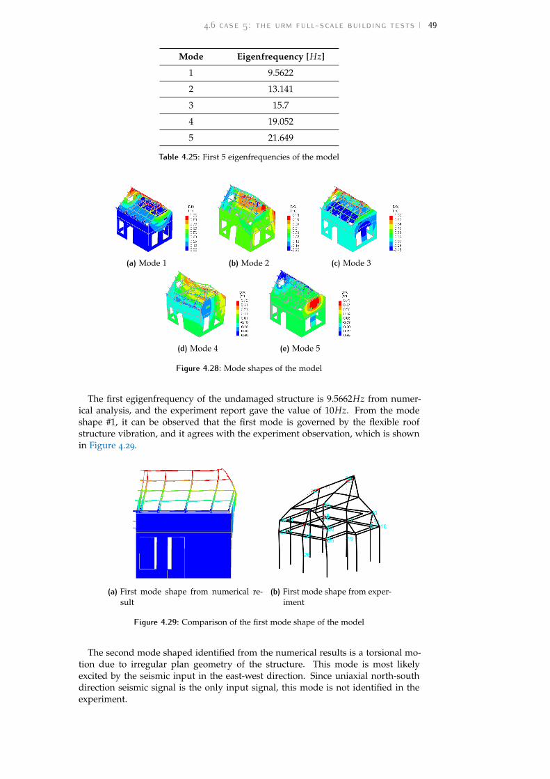
4.6 case 5: the urm full-scale building tests 49
Mode Eigenfrequency [Hz]
1 9.5622
2 13.141
3 15.7
4 19.052
5 21.649
Table 4.25: First 5 eigenfrequencies of the model
(a) Mode 1 (b) Mode 2 (c) Mode 3
(d) Mode 4 (e) Mode 5
Figure 4.28: Mode shapes of the model
The first egigenfrequency of the undamaged structure is 9.5662Hz from numer-ical analysis, and the experiment report gave the value of 10Hz. From the modeshape #1, it can be observed that the first mode is governed by the flexible roofstructure vibration, and it agrees with the experiment observation, which is shownin Figure 4.29.
(a) First mode shape from numerical re-sult
(b) First mode shape from exper-iment
Figure 4.29: Comparison of the first mode shape of the model
The second mode shaped identified from the numerical results is a torsional mo-tion due to irregular plan geometry of the structure. This mode is most likelyexcited by the seismic input in the east-west direction. Since uniaxial north-southdirection seismic signal is the only input signal, this mode is not identified in theexperiment.

50 cases studies: finite element model and analyses schemes
The third mode of the numerical result was identified during the experiment.In this vibration mode, not only the flexible roof structure, but also the masonrywalls, influence the mode shapes. The frequency identified in experiment is 18Hzand the numerical result is 15.7Hz. The difference may come from the fact thatthe real structure is stiffer than the FE model at the first floor level in the north-south direction due to additional anchors installed on the floor beams. Though, theoverall vibration mode, which involves significant deformation of masonry walls ofnorth and south sides, is similar, as shown in Figure 4.30.
(a) Second mode shape from numericalresult
(b) Second mode shape from ex-periment
Figure 4.30: Comparison of the second mode shape of the model
Seismic analysis in linear elastic phase
The preliminary seismic analyses using direct time integration methods are per-formed. The main purposes of these analyses are to have a first sight of the valida-tion of the model as well as the viability of two interested direct time integrationmethods: implicit Newmark method and explicit central difference method.
For such a complex structure, it is suggested to start with linear elastic materialproperty. According to the experimental results, when the structure subjected to thesignal SC1 100%, no visible crack and obvious nonlinear behavior were observedon the house, hence it can be assume that the house is almost remaining linearelastic. Therefore, all the materials, including masonry, are assumed to be linearelastic, and the signal SC1 100% was adopted. The Rayleigh damping was addedto the model according to the eigenvalue analysis and the cumulative effective massmethod mentioned in Section 4.5.
According to the experimental results, the following results are investigated: thedisplacement time history of the first floor (East and West sides) and of roof level;the positive and negative displacement envelopes recorded at first floor (East andWest sides) and at roof level; the hysteretic response in terms of base shear vs first-floor average displacement. As marked in Figure 4.31, the displacement of East sideis obtained by taking average value of nodes #5599 and #5619, and for West side,nodes #7174 and #5678. The roof displacement is obtained from node #10314.
First, the unconditionally stable implicit method is used. Consider the complexityof the structure, the time step is selected to be 0.05s, and the total analysis time tobe 20s. Slightly numerical damping is included in the Newmark method (β =0.3025, γ = 0.6). The displacement time history of first floor East side is shown inFigure 4.32. The other results of the implicit method are shown in Appendix A.

4.6 case 5: the urm full-scale building tests 51
Figure 4.31: Target nodes to obtain interested results
0 1 2 3 4 5 6 7 8 9 10 11 12 13 14 15 16 17 18 19 20
Time [s]
-0.06
-0.04
-0.02
0
0.02
0.04
0.06
0.08
Dis
pla
cem
ent
[mm
]
Relative displacement response at first floor East side
Experimental
Implicit method
(a) East side
Figure 4.32: Comparisons of displacements time history of the first floor East side
The results comparisons of the preliminary analysis using implicit method showthat results from numerical results generally agree with the experimental results.The displacement responses have very similar trends in both results. However, thenumerical results have slightly lower peak values for the first floor displacement re-sponse on both East and West sides, which can be also observed from the displace-ment envelope comparison, this is because the linear elastic material properties areassumed for the model while in the experiment nonlinear properties of the materialinfluence the response even without obviously visible crack. This can be proved bythe hysteretic curves of base shear versus average first floor displacement results,and it can be observed that much more energy was dissipated due to the nonlinear-ity in the experimental results than the numerical solution. Therefore, calibrationsof the model are still needed, but in general, the comparisons between results fromthe implicit method solution and the experimental solution verify the validity of theFE model.
Then, the explicit method was adopted for the analysis. However, due to theirregular geometry of the model and also high density meshes, it turns out thatmin∆tcrit is extremely small. Therefore the parameter in the explicit method∆tlim is used to force the time step adopted for the algorithm to become larger. Asa result, this will add artificial mass on the model and may change the dynamicproperty of the model.
Few analyses with different ∆tex were performed. The results of relative displace-ment response at first floor east side are given in Figure 4.33.

52 cases studies: finite element model and analyses schemes
Figure 4.33: Explicit method solution vs Experimental results
It can be observed that the results are unacceptable for explicit method. Thedisplacement is much larger than the experimental results, because the added massis too large compared to the original model mass. The artificial added mass ratiosfor different ∆tex, including a extra smaller one 5× 10⁻⁶, are shown in Figure 4.33.It shows that with decreasing added mass ratio, the solution of explicit methodis becoming better and better. However, the smallest explicit time step ∆tex =5× 10⁻⁶ shows that the ratio between artificial mass and total mass of the modelis 64%, which is unacceptably large, and the solution of such a time step is eitherunreasonable. Additionally, to investigate how is the distribution of elements whichhave added mass with time step ∆tex = 5× 10⁻⁶, positions of these elements arechecked in FE model, some typical added mass elements are shown in Appendix B.
All of these preliminary analyses results and discussions above turn out the ne-cessity of a simplified model of the house as well as a shorter duration of the load,in order to make explicit method run faster.
4.6.6 Simplified model
The simplifications will change the original properties of the structure. But con-sidering that the implicit method can obtain a reasonable results for the seismicanalysis, as well as the main focus of this research is compare the solutions fromimplicit method and explicit method, the comparisons for the simplified model willbe made between the solutions obtained from implicit method and explicit method.
The first simplification is removing the roof structure, because the roof structureprovides limited loading capacity to the structure which is subjected to the baseacceleration. Also, the roof structure is relatively light-weighted and unimportantto study the nonlinear behavior of the quasi-brittle masonry material.
Then, parts of masonry walls above the first floor level is removed too, becausethe out-of-plane stiffness of these walls are very low due to the absence of roofstructure and the out-of-plane failure of these walls will always occur as one canexpect. Moreover, these masonry walls have irregular shapes, removing them isalso good for a regular meshing.
Finally, the mesh size is increased to 0.2m to speed up the analysis. Particularly,the first floor structure is re-meshed in order to generally increase the mass (in theterm of mesh size) of these elements.
The simplified model of the house is shown in Figure 4.34. The other aspects ofthe model remain unchanged. The nonlinear behavior of the masonry is consideredin analyses for the rest of the part of this thesis. A list of element type and numberare shown in Table 4.26

4.6 case 5: the urm full-scale building tests 53
Figure 4.34: Simplified model of the house
Structurecomponents
Masonry wall& floor panel &
mass blocksfloor girders
Other timberbeams
Element typeCurved shell
element(Q20SH)
Class-III beamelement
(L12BEA)
Class-I beamelement(L12BE)
Integrationscheme
2× 2× 3 1-point 2-point
Mesh size 0.2m
Number ofelements
2301 379 15
Total Number ofnodes
2481
Total number ofelements
2695
Table 4.26: List of used element types and mesh properties in simplified model
Modified input seismic signal
The input signal is also modified so that the most interested nonlinear behaviorof the structure could be activated. According to the report, obvious cracks areobserved after the signal SC2 400%, where the building experienced a substantiallevel of damage. Hence, the signal SC2 400% was adopted in this case. Similarto the Case 4 in Section 4.5, the input acceleration time history was selected tobe the interval between 1s− 10s of signal SC2 400%, because the most significantstrong acceleration is included in this interval and the rest part of the signal haslimited influence on the nonlinear behavior of the structure. Therefore, the inputacceleration time history is the same as one in Case 4, as shown in Figure 4.14b.
Analyses schemes
For the simplified model, the eigenfrequency analysis is needed to have a insightview of the dynamic property of the structure. Also, according to the eigefrequencyanalysis, the Rayleigh damping parameter and the output time interval could bedetermined. The first natural frequency of the model is 13.4Hz, and the Rayleigh

54 cases studies: finite element model and analyses schemes
parameters, according to the cumulative effective mass method, are chosen as a =8.1 and b = 0. The output time interval is selected as 0.005s, which is much smallerthan the first natural period of the structure.
Then implicit method with lumped mass and damping matrices and no intro-duced numerical damping is used to perform the transient analysis with a loadduration of 9s. The analysis scheme using implicit Newmark method is listed inTable 4.27.
Implicit method Newmark method
Time step ∆tIm 0.005s
Total steps NIm 1800
Newmark parameter β = 0.25 , γ = 0.5
Iteration method Regular Newton-Raphson method
Convergence norm Displacement or force
Convergence tolerance 0.01
Maximum iteration number 200
Line search Yes
Mass Matrix and damping matrix Lumped
Table 4.27: Transient analyses schemes for implicit Newmark method
The minimum critical time step in the simplified model is min∆tcrit = 1.8485×10⁻⁶s. Since this time step is still pretty small, few analyses with slightly largerexplicit time steps ∆tex are performed, and one analysis with this min∆tcrit isperformed finally. The analyses schemes are given in Table 4.28
Sub-cases Sub-case 1 Sub-case 2 Sub-case 3 Sub-case 4
min∆tcrit 1.8485× 10⁻⁶s
∆tlim,i 5× 10⁻⁵s 10−5s 5× 10⁻⁶s 10−6s
∆tred 0.95
∆tubs 10−3s
∆tO 0.005s
∆tex,i 5× 10⁻⁵s 10−5s 5× 10⁻⁶s 1.756× 10⁻⁶s
Nsub,i 100 500 1000 2847
Table 4.28: Transient analyses schemes for explicit method

5 C A S E S S T U DY: R E S U LT SC O M PA R I S O N S A N D D I S C U S S I O N S
5.1 overviewIn this chapter, the numerical solutions of the transient analyses described in theChapter 4 for every case are presented. The comparisons between the solutionof implicit and explicit method are made. For convenience, a list of the analysesschemes for each case is reviewed again. The comparison for linear cases are mainlyin terms of displacement response, and for nonlinear cases additional aspects, suchas crack patterns, hysteretic curves, are also considered. Necessary discussions weremade to have a better understanding and interpretation of the results. Finally, theseresults and discussions will form the answers to the research questions proposed atthe start of this thesis.
5.2 case 1In Case 1, the mid-span (node #8) deflection of the beam is selected as the interestedresults, as shown in Figure 5.1. The deflection time history of node #8 will be com-pared between analytical solution, implicit method solution and explicit solution.
Figure 5.1: The interested point (node #8) on the simply-supported beam
5.2.1 Analytical solution
The reference solution of the steady-state response of the beam is obtained by solv-ing the classical governing equation of the beam.
The equation of the motion of the beam is:
ρA∂2y∂t2 + EI
∂4y∂t4 = 0 (5.1)
The boundary conditions are:
x = 0 : y− = ∂2y−/∂x2 = 0
x = L : y+ = ∂2y+/∂x2 = 0(5.2)
The interface conditions are:
x = x0 : y− = y+
∂y−/∂x = ∂y+/∂x
∂2y−/∂x2 = ∂2y+/∂x2
EI(∂3y+/∂x3 − ∂3y−/∂x3) = Psin(Ωt)
(5.3)
55

56 cases study: results comparisons and discussions
The steady-state solution is assumed to be:
y(x, t) = Y(x)sin(Ωt) (5.4)
By substituting the assumed solution into governing equations, we can get the gen-eral solution in the frequency domain as:
Y−(x) = A−cosh(βx) + B−sinh(βx) + C−cos(βx) + D−sin(βx)
Y+(x) = A+cosh(βx) + B+sinh(βx) + C+cos(βx) + D+sin(βx)(5.5)
where β is defined as β4 =ρAEI
Ω2.
Equation 5.5 has 8 unknowns, by substituting these general solution into 4 bound-ary conditions and 4 interface conditions, they can be solved. Then, according tothe equation 5.4, the analytical solution y(x, t) can be obtained for any location onthe beam at any time. The Figure 5.2 shows the steady-state response of mid-spanof the beam in 1 seconds duration.
0 0.1 0.2 0.3 0.4 0.5 0.6 0.7 0.8 0.9 1
Time [s]
-2
-1.5
-1
-0.5
0
0.5
1
1.5
2
Dis
pla
cem
ent
[mm
]
10-3 Analytical displacement response at mid-span of the beam
Figure 5.2: The analytical solution for mid-span deflection time history
5.2.2 Numerical solutions
Review of analyses schemes
Analyses Damping ∆tO [s] min∆tcrit [s] ∆tex [s]
Implicit No 0.001 − −Explicit
Sub-case 1No 0.001 1.50756× 10⁻⁵ 1.43218× 10⁻⁵
ExplicitSub-case 2
No 0.001 1.50756× 10⁻⁵ 10−5
Table 5.1: Review of transient analysis scheme for Case 1
Solutions
First, a simple eigenfrequency analysis was performed to identify the natural fre-quency of the beam.The result turns out the first natural frequency is 49.69Hz.
The implicit method solution at mid-span (node #8) according to the analysisscheme in Table 4.3 is plotted in Figure 5.3a. The explicit method solutions ac-cording to analysis scheme Table 4.4, which include two sub-cases, are plotted inFigure 5.3b.

5.3 case 2 57
0 0.1 0.2 0.3 0.4 0.5 0.6 0.7 0.8 0.9
Time [s]
-2
-1
0
1
2
Dis
pla
cem
ent
[mm
]
10-3Displacement response at mid-span (node #8)
(a) The implicit method solution
0 0.1 0.2 0.3 0.4 0.5 0.6 0.7 0.8 0.9
Time [s]
-2
-1
0
1
2
Dis
pla
cem
ent
[mm
]
10-3Displacement response at mid-span (node #8)
Explicit Sub-case 1
Explicit Sub-case 2
(b) Two explicit sub-cases’ solutions
Figure 5.3: Numerical solutions for mid-span deflection time history
5.2.3 Comparison of the solutions
Since it has been observed that the two explicit sub-cases have exactly the sameresult, the sub-case 1 which uses the minimum critical time step was used for thefollowing comparisons. The three solutions obtained from different methods arecompared together with zooming in different time history intervals, as shown inFigure 5.4.
0 0.05 0.1 0.15 0.2
Time [s]
-2
-1
0
1
2
Dis
pla
cem
ent
[mm
]
10-3 Displacement response between 0-0.2s
Analytical
Implicit
Explicit sub-case 1
(a) Time interval 0− 0.2s
0.6 0.65 0.7 0.75 0.8 0.85 0.9
Time [s]
-2
-1
0
1
2
Dis
pla
cem
ent
[mm
]
10-3 Displacement response between 0.6-0.9s
Analytical
Implicit
Explicit sub-case 1
(b) Time interval 0.6− 0.9s
Figure 5.4: Comparison of the solutions in different time intervals
It can be observe that both direct time integration methods accurately reproducethe steady-state displacement response at the mid-span in a short time after theload was applied. In the time interval 0− 0.2s slight differences are observed innumerical solutions. This is the first vibration mode of the beam, corresponding tothe first natural frequency 49.96Hz. Since the steady-state response needs time toreach, the transient effect shows up at the beginning of the analysis. In the timeinterval 0.6− 0.9s, three solutions are fully overlapped due to the damping effect.
Moreover, the same results of two explicit method sub-cases shows that oncethe stability condition is reached in the linear elastic system, which means themin∆tcrit is used for the explicit algorithm, the explicit method could accuratelygenerate the displacement response of the structure, the further decrement for theexplicit time step is not necessary.
5.3 case 2
In Case 2 (Section 4.3), the mid-span (node #1) is selected for the results compari-son. The node #1 is the node on which the transient load was applied, as shownin Figure 5.5. Three different time steps are used to generate the output of thedisplacement response of the node #1, which are 25µs, 50µs and 100µs. The anal-yses schemes are described in Table 4.7 and Table 4.8. The reference solutions are

58 cases study: results comparisons and discussions
calculated in ABAQUS using implicit solver with slight numerical damping. Thecomparison of each case is made in the following section.
Figure 5.5: The interested point (node #1) in FE model
Review of analyses schemes
Analyses Damping ∆tO [µs] min∆tcrit [s] ∆tex [s]
ImplicitSub-case 1
No 25 − −
ImplicitSub-case 2
No 50 − −
ImplicitSub-case 3
No 100 − −
ExplicitSub-case 1
No 25 7.21291× 10⁻⁷ 6.85226× 10⁻⁷
ExplicitSub-case 2
No 50 7.21291× 10⁻⁷ 6.85226× 10⁻⁷
ExplicitSub-case 3
No 100 7.21291× 10⁻⁷ 6.85226× 10⁻⁷
Table 5.2: Review of transient analysis scheme for Case 2
5.3.1 Sub-case 1: solutions of time step 25µs
The solutions of sub-case 1 from different methods with using output time step of25µs are given in Figure 5.6.
0 1 2 3 4 5
Time [s] 10-3
0
0.005
0.01
0.015
0.02
Dis
pla
cem
ent
[m]
Displacement response at the midspan (25 s)
Reference
Implicit sub-case 1
Explicit sub-case 1
Figure 5.6: The displacement response at node #1 with time step 25µs
With output time step 25µs, the solution are accurately generated in all methods,the results are quite close to each other and no obvious difference is observed.
5.3.2 Sub-case 2: solutions of time step 50µs
A larger output time step is used in sub-case 2, which is 50µs. The comparison of so-lutions are shown in Figure 5.7 The results are still match each other in general, but

5.3 case 2 59
0 1 2 3 4 5
Time [s] 10-3
0
0.005
0.01
0.015
0.02
Dis
pla
cem
ent
[m]
Displacement response at the midspan (50 s)
Reference
Implicit sub-case 2
Explicit sub-case 2
Figure 5.7: The displacement response at node #1 with time step 50µs
slight difference starts to show up in the comparison. A larger amplitude of highfrequency component is contained in the explicit solution. The implicit and refer-ence solution are more closer to each other. However, since the reference solution isalso calculated by implicit method, this can be expected to happen.
5.3.3 Sub-case 3: solutions of time step 100µs
A much larger time step of 100µs is used for sub-case 3. The results are shown inFigure 5.8. Even with much coarser resolution of the solution, the explicit solution
0 1 2 3 4 5
Time [s] 10-3
0
0.005
0.01
0.015
0.02
Dis
pla
cem
ent
[m]
Displacement response at the midspan (100 s)
Reference
Implicit sub-case 3
Explicit sub-case 3
Figure 5.8: The displacement response at node #1 with time step 100µs
still remains the information about high frequency components. However, in theimplicit solutions, these information has been mainly lost.
5.3.4 Comparisons of solution from different time steps
The comparison between three implicit sub-cases are given in Figure 5.9a, and sim-ilar comparison is made for three explicit sub-cases, shown in Figure 5.9b.
0 1 2 3 4 5
Time [s] 10-3
0
0.005
0.01
0.015
0.02
Dis
pla
cem
ent
[m]
Comparison of 3 implicit sub-cases
Sub-case 1( t=25 s)
Sub-case 2( t=50 s)
Sub-case 3( t=100 s)
(a) Implicit sub-cases
0 1 2 3 4 5
Time [s] 10-3
0
0.005
0.01
0.015
0.02
Dis
pla
cem
ent
[m]
Comparison of 3 Explicit sub-cases
Sub-case 1( tO
=25 s)
Sub-case 2( tO
=50 s)
Sub-case 3( tO
=100 s)
(b) Explicit sub-cases
Figure 5.9: Comparisons of solutions from different time steps

60 cases study: results comparisons and discussions
It can be observed that the time step has very significant influence on the implicitmethod solutions. The amplitude of the displacement response as well as the highfrequency components are changing due to the changes of the time step. The largertime step used, the less of high frequency components are reproduced. This isbecause the time step for implicit method is too large to capture the high frequencywave traveling through the nodes, so the information is lost. Though, the implicitmethod is unconditionally stable, the accuracy will be lost due to the large timestep.
While in the explicit method solution, almost no difference could be observedin three sub-cases. This is because the explicit algorithm actually calculates thesolution at the min∆tcrit = 7.21291× 10⁻⁷s, which is determined to be able torepresent the highest frequency wave traveling through the element nodes, accord-ing to the CFL stability condition. So, even with different output time step ∆tO, theaccurate response is always calculated, the only influence of ∆tO is the resolutionof the solution. Once the resolution is good enough to show the high frequencyvibration modes, the results could be considered to be accurate.
5.4 case 3The Case 3 investigates the response of simply-supported thin plate to out-of-planetransient distributed force, as described in Section 4.4. The reference solution isgiven at the middle point (node #1) of the plate in Maguire et al. [1993], as shown inFigure 5.10. The numerical solution of peak displacement in out-of-plane direction,peak stress and their corresponding time points will be compared with the referencesolution in Maguire et al. [1993]. The analyses schemes are described in Table 4.10
and Table 4.11.
Figure 5.10: The interested point (node #1) in FE model
Review of analyses schemes
Analyses Damping ∆tO [s] min∆tcrit [s] ∆tex [s]
ImplicitSub-case 1
RayleighDamping
0.01 − −
ImplicitSub-case 2
RayleighDamping
0.002 − −
ExplicitSub-case 1
RayleighDamping
0.01 1.4597× 10⁻⁴ 1.38672× 10⁻⁴
ExplicitSub-case 2
RayleighDamping
0.002 1.4597× 10⁻⁴ 1.38672× 10⁻⁴
Table 5.3: Review of transient analysis scheme for Case 3

5.4 case 3 61
5.4.1 Eigenfrequencies
The first eight eigenfrequencies and the corresponding mode shapes are identifiedfor the FE model, as shown in Figure 5.11. The comparison of the identified eigen-frequencies and reference values are listed in Table 5.4. The results show goodagreement with the reference solution.
(a) Mode 1, 2.4026Hz (b) Mode 2 & 3, 6.1853Hz (c) Mode 4, 9.9345Hz
(d) Mode 5 & 6, 13.160Hz (e) Mode 7 & 8, 16.849Hz
Figure 5.11: First eight eigenfrequencies and the corresponding mode shapes
EigenfrequenciesReference
[Hz]Identified
[Hz]
f1 2.398 2.4026
f2 & f3 6.1195 6.1853
f4 9.89 9.9345
f5 & f6 12.845 13.160
f7 & f8 16.582 16.849
Table 5.4: Identified eigenfrequencies vs reference values
According to the eigenfrequencies of the model, two output time steps which are0.01s and 0.002s, the first one guarantees the first mode will be generated accuratelyand the second one provides the possibility for up to eighth mode.
5.4.2 Displacement time history in out-of-plane direction
The solution of displacement time history of node #1 in out-of-plane direction fromimplicit method is shown in Figure 5.12a and from explicit method is shown inFigure 5.12b. Almost no difference could be observed in implicit sub-cases, neitherin explicit sub-cases. The displacement response could be calculated accurately inboth methods.
5.4.3 Stress σxx time history
The solution of displacement time history of node #1 in out-of-plane direction fromimplicit method is shown in Figure 5.12a and Figure 5.12b show the stress σxx timehistory solution at node #1 calculated by implicit and explicit method respectively.
In the stress results, differences are observed between implicit sub-cases, the so-lution from different time steps show different high frequency contents. This mayimply that high vibration mode ares excited even though it doesn’t clearly show

62 cases study: results comparisons and discussions
0 0.2 0.4 0.6 0.8 1 1.2 1.4 1.6 1.8 2
Time [s]
-3.5
-3
-2.5
-2
-1.5
-1
-0.5
0
Dis
pla
cem
ent
[m]
10-3 Displacement response at the middle point
Implicit sub-case 1( t=0.01s)
Implicit sub-case 2( t=0.002s)
(a) Implicit sub-cases
0 0.2 0.4 0.6 0.8 1 1.2 1.4 1.6 1.8 2
Time [s]
-3.5
-3
-2.5
-2
-1.5
-1
-0.5
0
Dis
pla
cem
ent
[m]
10-3 Displacement response at the middle point
Explicit sub-case 1( tO
=0.01s)
Explicit sub-case 2( tO
=0.002s)
(b) Explicit sub-cases
Figure 5.12: Comparisons of displacement time history of node #1 in out-of-plane direction
0 0.2 0.4 0.6 0.8 1 1.2 1.4 1.6 1.8 2
Time [s]
-0.5
0
0.5
1
1.5
2
2.5
Str
ess
xx [
N/m
2]
106 Stress
xx at the middle point
Implicit sub-case 1( t=0.01s)
Implicit sub-case 2( t=0.002s)
(a) Implicit sub-cases
0 0.2 0.4 0.6 0.8 1 1.2 1.4 1.6 1.8 2
Time [s]
-0.5
0
0.5
1
1.5
2
2.5
Str
ess
xx [
N/m
2]
106 Stress
xx at the middle point
Explicit sub-case 1( tO
=0.01s)
Explicit sub-case 2( tO
=0.002s)
(b) Explicit sub-cases
Figure 5.13: Comparisons of stress σxx time history of node #1
in the displacement response. While, the explicit sub-cases have exactly the samestress time history, but still, higher vibration mode is observed which isn’t repro-duced in displacement response.
5.4.4 Comparisons and discussions
The peak displacement and peak stress values in implicit and explicit solutions arecompared with the reference solution, as well as the corresponding time points. Theresults are given in Table 5.5.
Peak displacement Peak stressδp (mm) tp (s) σxx (N/mm2)
Reference solution 3.507 0.216 2.484
Implicit solution 3.472 0.218 2.353
Explicit solution 3.463 0.210 2.355
Table 5.5: Comparison of peak response
The numerical solutions show good agreement with the reference solution. Thedifference between the peak displacements is smaller than 1.5%, and the time pointsfor peak values are also very close. The peak stress has about 5% deviation, itmay cause from the influence of high frequency vibration mode in the numericalsolutions, but they are still very close to each other.
To investigate the difference in the stress σxx time history, the implicit solutionsand explicit solution are plotted together in Figure 5.14. In addition, the Fast FourierTransform (FFT) of the σxx time history is calculated and plotted in Figure 5.15.

5.4 case 3 63
0 0.2 0.4 0.6 0.8 1 1.2 1.4 1.6 1.8 2
Time [s]
-0.5
0
0.5
1
1.5
2
2.5
Str
ess
xx [
N/m
2]
106 Stress
xx at the middle point
Implicit sub-case 1( t=0.01s)
Implicit sub-case 2( t=0.002s)
Explicit sub-case 1( tO
=0.01s)
Figure 5.14: Comparison between implicit and explicit solutions of σxx
0 2 4 6 8 10 12 14 16
Frequency [Hz]
0
0.2
0.4
0.6
0.8
1
Norm
ali
zed
magn
itu
de
FFT of the stress xx
response
Implicit sub-case 1
Implicit sub-case 2
Explicit sub-case 1
(a) Implicit sub-cases vs explicit sub-case1
0 2 4 6 8 10 12 14 16
Frequency [Hz]
0
0.2
0.4
0.6
0.8
1
Norm
ali
zed
magn
itu
de
FFT of the stress xx
response
Implicit sub-case 1
Implicit sub-case 2
Explicit sub-case 2
(b) Implicit sub-cases vs explicit sub-case2
Figure 5.15: Comparisons of FFT of stress σxx time history
Figure 5.14 shows that the explicit solution has very close results to implicit sub-case 2, which has the smaller time step than implicit sub-case 1. Though, the ex-plicit has a lower resolution of the solution, which is ∆tO = 0.01s, compared tothe implicit sub-case 2 with ∆t = 0.002s, it still contains accurate high frequencyinformation, which is better than the implicit sub-case 1.
The comparisons of FFT show that the dominant frequency component in thestress time history is 2.333Hz, which is corresponding with the first natural freevibration frequency 2.398Hz, the difference is come from the Rayleigh dampingincluded in the model. The different amplitudes at this frequency come from thedifferent resolutions of the signals, as a result lower resolution of the signal hasmore leakage in the Fourier spectrum. It can be proved in Figure 5.15a and Fig-ure 5.15b, the amplitudes of the first peak of explicit solutions are the same withthe corresponding resolution of implicit solution, in this case, the output time step.
However, another important peak value occurs at around 11.5Hz to 12.5Hz, whichis corresponding to the 5th and 6th vibration modes, again, the value is reduceddue to damping. The implicit sub-case 1 has peak value at 11.59Hz, the implicitsub-case 2 at 12.12Hz, the explicit cases at 11.71Hz. This is the reason why differenthigh frequency vibrations occurred in stress response time history. It turns out thatwith smaller time step, the implicit method could generate high frequency vibrationmore accurately, while the explicit is not influenced by that. The larger time step inimplicit method tends to make this frequency shift towards left, i.e. smaller, whichwill lead to inaccurate representation of high frequency mode vibration.
The reason why only first and 5th (or 6th) modes are excited is that transientdistributed load is applied on the all plate surface, so the symmetric modes are moreeasily to be activated. However, since the energy contained in the high frequencymode is so low, it is hard to observe it in displacement response.

64 cases study: results comparisons and discussions
5.5 case 4
The results of the Case 4 (Section 4.5) will be presented in two parts, the first partis the in-plane shear-compression quasi-static analysis results and the second partis the in-plane seismic analysis results. The in-plane quasi-static analysis aims tovalidate the material parameters in the FE model and study the nonlinear behaviorof the masonry wall. The seismic analysis will take into account the transient effectof seismic loading and investigate the performance of implicit and explicit methodfor nonlinear quasi-brittle material.
5.5.1 In-plane shear-compression test
As described in Section 4.5.2 and Figure 4.9, the wall is subjected to prescribeddisplacement applied at the top edge. Since the typing is used in the model, theprescribed displacement is directly applied at the master nodes, as a result, the baseshear force could be obtained either from reaction forces of nodes at bottom edgesor from the virtual support reaction force at the master node.
The in-plane tests include a monotonic pushover analysis with eigenfrequencycheck and a cyclic pushover analysis. The results of capacity curves and hysteresiscurves are generated and compared to the experimental results. Also, the nonlinearbehavior of the model and its influence on the eigenfrequency are also discussed.
Monotonic pushover results
As shown in Table 4.16, a prescribed horizontal displacement of 34.2mm was ap-plied at the master node on the model. The capacity curve in terms of displacementversus base shear force is plotted in Figure 5.16a, and the first eigenfrequency evo-lution during the monotonic pushover process is plotted in Figure 5.16b.
0 5 10 15 20 25 30 35
Horizontal displacement [mm]
0
20
40
60
80
100
Ba
se s
hea
r fo
rce
[kN
]
Capacity curve of the maosnry wall
Base shear shear force
Frequency check points
(a) Capacity curve
0 5 10 15 20 25 30 35
Horizontal displacement [mm]
80
100
120
140
160
180
200
220
Fir
st e
igen
freq
uen
cy [
Hz]
Eigenfrequency evolution of the maosnry wall
(b) First eigenfrequency evolution
Figure 5.16: Monotonic pushover results
The maximum shear capacity in numerical results is 94.67kN, which is quite closeto the reference value obtained from cyclic pushover test 92.52kN in positive direc-tion and 92.55kN in negative direction. Moreover, the softening behavior is alsoshown in the capacity curve due to the crack in the model. Hence, the stiffness ofthe material is reduced and the natural frequency of the structure as well as theelement is decreased, as proved in the first frequency evolution result. The firstnatural frequency drops from 201.3Hz to around 99.27Hz at the end. Few figures ofthe crack width evolution during the pushover procedure together with the corre-sponding first natural frequency are shown in Figure 5.17 to illustrate this softeningbehavior.

5.5 case 4 65
(a) (b) (c) (d) (e)
Figure 5.17: Crack evolution with corresponding top displacement Dx and frequency f : (a)Dx = 3.428mm, f = 124.8Hz; (b) Dx = 13.712mm, f = 111Hz; (c) Dx =27.424mm, f = 104.6Hz; (d) Dx = 34.28mm, f = 99.27Hz (e) The legend.
Cyclic pushover results
The cyclic pushover analysis scheme is given in Table 4.17. The hysteresis curveof horizontal displacement versus base shear force are plotted in Figure 5.18 withcomparing to the experimental result.
Figure 5.18: The hysteresis curve of masonry wall
The numerical results have a good agreement with the experimental results. Theinitial stiffness is almost the same. The maximum loading capacity in positiveand negative direction of numerical results are +93.45kN and −93.93kN, whichare slightly higher than experimental results of +92.52kN and −92.55kN, the dif-ference is around 1%. The decrease of the capacity with increasing cycles and theunloading-reloading curve of the numerical results match the experimental resultsvery well. However, the stiffness at the end of the loading shows some differences,it might be caused by the fact the wall in the experimental test are exhibits intensivetoe crushing at the base in the end of loading cycles, so that the structure is unableto carry load anymore. This failure of the wall can be observed from the curvesof last three cycles in the experimental results. Most of the energy is dissipated inthese three cycles as well.
The masonry wall model first cracked at the bottom edge and the bricks belowthe wall-top beam. At this point, the pier has a pure rocking behavior, until thefirst diagonal cracks appear above the base. Then the specimen exhibits intensivetoe crushing mechanism at the base. After that, diagonal crack appears in the tophalf of the pier, rendering the wall is unable to carry vertical load anymore. Thefailure mode is a hybrid failure mode, which means the rocking mechanism and

66 cases study: results comparisons and discussions
toe crushing first happened and after the maximum flexural capacity of the pierreached, then shear failure occurs. In general, this crack evolution and the failuremode are shared between test results and numerical results. Few illustrations of thecrack width evolution are shown in Figure 5.19.
(a) +1mm (b) −1.44mm (c) +4mm (d) −5mm
(e) +6.5mm (f ) −8mm (g) +13.5mm (h) −27mm
(i) +34.2mm (j) −34.2mm (k)
Figure 5.19: Crack width evolution with corresponding top displacement

5.5 case 4 67
5.5.2 In-plane seismic analysis
The Section 4.5.3 has given the detailed information about the modified FE model,seismic input signal and the analyses schemes. The node #2 are selected to showthe results comparisons for this model, as shown in Figure 5.20.
Figure 5.20: The interested node #2 on the modified FE model for seismic analysis
Review of analyses schemes
Analyses Damping ∆tO [s] min∆tcrit [s] ∆tex [s]
ImplicitRayleighDamping
0.005 − −
ExplicitSub-case 1
RayleighDamping
0.005 4.50268× 10⁻⁵ 4.27754× 10⁻⁵
ExplicitSub-case 2
RayleighDamping
0.005 4.50268× 10⁻⁵ 5× 10⁻⁶
Table 5.6: Review of transient analysis scheme for Case 4
Eigenfrequency analysis
The eigenfrequencies and mode shapes are first identified for the mode. Sincethe double-fixed boundary condition was changed to free at top edge with a highdensity steel beam, the eigenfrequency was reduced a lot compared to the modelin quasi-static analysis. The mode shapes and the corresponding eigenfrequenciesrelated to the vibration in seismic excitation’s direction are presented in Figure 5.21.
Compared with the Fourier spectrum of the input seismic signal (Figure 4.15), inwhich most of the energy was contained by the frequency components below 12Hz,it can be predicted that the response of the structure to this seismic input will begoverned by the first vibration mode.
Displacement responses of node #2
The transient analysis scheme using implicit method was performed according toTable 4.19, and explicit method according to Table 4.20. The relative displacementtime history of node #2 with respect to the base is plotted in Figure 5.22a andFigure 5.22b.

68 cases study: results comparisons and discussions
(a) 10.707Hz (b) 85.240Hz (c) 217.050Hz
Figure 5.21: Eigenfrequencies and mode shapes
0 0.5 1 1.5 2 2.5 3 3.5 4 4.5 5 5.5 6 6.5 7 7.5 8 8.5 9
Time [s]
-2.5
-2
-1.5
-1
-0.5
0
0.5
1
1.5
2
Dis
pla
cem
ent
[mm
]
Relative displacement time history of node #2
(a) Implicit method solution
0 0.5 1 1.5 2 2.5 3 3.5 4 4.5 5 5.5 6 6.5 7 7.5 8 8.5 9
Time [s]
-2.5
-2
-1.5
-1
-0.5
0
0.5
1
1.5
2
Dis
pla
cem
ent
[mm
]
Relative displacement time history of node #2
Sub-case 1: tex
=4.27754E-5
Sub-case 2: tex
=5E-6
(b) Explicit method solutions
Figure 5.22: Relative displacement time history of node #2 with respect to the base
Both methods produced reasonable displacement response. Two explicit sub-cases with different explicit time step ∆tex provide the same solution again, becausethey are both equal or smaller than the min∆tcrit, in another word, satisfy the CFLstability condition. Differences could be observed in the results. The comparisonand discussion will be made later with referring to other aspects of the results.
Eigenfrequency evolution in seismic analysis
The first eigenfrequency of the masonry wall was checked every 0.5s through theseismic analysis. Evolution of the first eigenfrequency is plotted in Figure 5.23,together with the relative displacement of node #2 at every time point.
0 0.5 1 1.5 2 2.5 3 3.5 4 4.5 5 5.5 6 6.5 7 7.5 8 8.5 9
Time [s]
4
5
6
7
8
9
10
11
12
Fre
qu
ency
[H
z]
First natural frequency vs Time
First natural frequency
Initial first natural frequency value
0 0.5 1 1.5 2 2.5 3 3.5 4 4.5 5 5.5 6 6.5 7 7.5 8 8.5 9
Time [s]
-2
-1
0
1
2
Dis
pla
cem
ent
[mm
]
Relative displacement time history of node #2 (Implicit)
Implicit solution
Frequency check points
Figure 5.23: Evolution of the first eigenfrequency of the structure and relative displacementsof node #2 at corresponding time points

5.5 case 4 69
The results show that the first natural frequency didn’t surpass the value whenstructure is in linear elastic phase. The values of the first natural frequencies dur-ing the seismic analysis is calculated of the current deformation or crack state ofthe material, which means at the moment when all cracks are closed, the naturalfrequency reaches the value of linear elastic phase, and when cracks open againthe material has softer stiffness and frequency decreases. Therefore, it can concludethat for material has softening behavior, the critical time step for explicit methoddetermined based on the linear elastic phase is always safe and satisfy the CFLstability conditions.
Hysteresis curve of base shear force versus relative displacement of node #2
The base shear force are calculated by summing up the nodal reaction force at thebase edge of the model. The hysteresis curves of base shear force versus relativedisplacement of node #2 are plotted in Figure 5.24.
-2.5 -2 -1.5 -1 -0.5 0 0.5 1 1.5 2
Relative displacement [mm]
-60
-50
-40
-30
-20
-10
0
10
20
30
40
50
60
Base
sh
ear
forc
e [k
N]
Base shear vs Relative displacement of node #2
(a) Implicit method solution
-2.5 -2 -1.5 -1 -0.5 0 0.5 1 1.5 2
Relative displacement [mm]
-60
-50
-40
-30
-20
-10
0
10
20
30
40
50
60
Base
sh
ear
forc
e [k
N]
Base shear vs Relative displacement of node #2
Sub-case 1: tex
=4.27754E-5
Sub-case 2: tex
=5E-6
(b) Explicit method solutions
Figure 5.24: Hysteresis curve of base shear force versus relative displacement of node #2
The hysteresis curves from both methods have good agreement with each otheron maximum shear force, energy dissipation and reloading-unloading behaviors.The explicit sub-cases show the same results again. However, the explicit solutionsshow much smoother than the implicit solution, in which slightly chaos values oc-cur after the largest hysteresis loop. This implies that it is hard for implicit methodto reach convergence criterion after the strong peak of the seismic signal.
5.5.3 Comparisons and discussions
Since the explicit sub-cases get the same solution, therefore the sub-case 1 is usedfor the following comparisons.
First, the comparison of displacement obtained from implicit method and explicitmethod are plotted together inFigure 5.25. Based on comparison, two time intervalsare zoomed in to show better views of the differences in response, plotted in Fig-ure 5.26a and Figure 5.26b. Fast Fourier Transform (FFT) is also applied on bothsolutions, as shown in Figure 5.26c.

70 cases study: results comparisons and discussions
0 0.5 1 1.5 2 2.5 3 3.5 4 4.5 5 5.5 6 6.5 7 7.5 8 8.5 9
Time [s]
-2.5
-2
-1.5
-1
-0.5
0
0.5
1
1.5
2
Dis
pla
cem
ent
[mm
]
Relative displacement time history of node #2
Implicit
Explicit
Figure 5.25: Comparisons between implicit and explicit method solutions of relative dis-placement time history of node #2
1.5 2 2.5 3 3.5 4 4.5 5
Time [s]
-2.5
-2
-1.5
-1
-0.5
0
0.5
1
1.5
2
Dis
pla
cem
ent
[mm
]
Relative displacement time history of node #2
Implicit
Explicit
(a) Time interval 1.5s− 5s
7.5 8 8.5 9
Time [s]
-2.5
-2
-1.5
-1
-0.5
0
0.5
1
1.5
2
Dis
pla
cem
ent
[mm
]
Relative displacement time history of node #2
Implicit
Explicit
(b) Time interval 7.5s− 9s
0 1 2 3 4 5 6 7 8 9 10 11 12 13 14 15
frequency [hz]
0
0.2
0.4
0.6
0.8
1
Norm
ali
zed
magn
itu
de
Fourier Spectrum
Implicit
Explicit
Input signal
(c) Fourier spectra
Figure 5.26: Differences in displacement responses and Fourier spectra
The differences show after the peak displacement response, the explicit solutionshows larger amplitude vibration after the peak response than the implicit solu-tion, this can be observed either in time interval of 1.5s− 5s or 7.5s− 9s. Then, theamplitude difference gradually disappears if no other peak arrives. This impliesthat more energy was dissipated in implicit method solution for the strong baseacceleration than the explicit solution. This can be proved in the Fourier spectraof the response. Compared with the spectra with the input seismic signal, both so-lutions include the same dominant frequencies contents of the input signal, whichis between 1− 4Hz. Moreover, the responses also have the first natural frequencycontent at around 9.5Hz, the value is slightly smaller because the damping is in-troduced. That means the first natural mode was activated by the seismic signal,however, the explicit spectrum has mush larger magnitudes around the first natu-ral frequency than implicit spectrum. So, in total, the energy contained in explicit

5.5 case 4 71
spectrum is larger, because the implicit dissipated more energy due to the nonlinearbehavior of the model.
To have a insight view of the nonlinear behavior in the seismic response, fewfigures about crack pattern, which is indicated by the state parameter NCRACK = 1(in this case red color), at different time point during the time interval 1.5s− 2.5sare presented in Figure 5.27.
(a) 1.755s (b) 1.845s (c) 1.885s (d) 2.500s (e)
(f) 1.755s (g) 1.845s (h) 1.885s (i) 2.500s (j)
Figure 5.27: Crack patterns development during 1.5s− 2.5s: (a)-(d) implicit solutions; (e)-(h)explicit solutions
It can be observed that the implicit solution has more cracks occur than explicitsolution during the strong peak acceleration of the seismic signal, therefore, moreenergy is dissipated through these cracks for implicit solution.
The comparison of the hysteresis curves plotted in Figure 5.28 also show thisdifference in energy dissipation. Though, the difference are not obvious, but still itcorresponds to the nonlinear behavior of the model.
Figure 5.28: Comparisons between implicit and explicit method solutions of hysteresiscurves of base shear vs relative displacement
In general, it can be concluded that for this masonry wall model with quasi-brittlematerial properties, both implicit and explicit methods could generate reasonablenonlinear dynamic response. The peak displacement responses are close to eachother for the solutions from both methods. Similar crack patterns were observedduring the seismic analysis. The energy dissipated due to the nonlinear behaviorcan be represented in the hysteresis curves.

72 cases study: results comparisons and discussions
However, slightly differences in nonlinear dynamic response under intense baseacceleration are observed. The explicit method solution show less cracks and lessenergy dissipation than the implicit method solution, meanwhile, the displacementsresponses after the peak displacement are also larger because less material crackedor failed. The difference could be resulted from the fact that implicit method mayhave problems to reach the convergence criteria when significant nonlinear behaviorwas activated due to the strong motion of the base. The chaos part in the hysteresiscurve of implicit solution provide some clues for this reason. The explicit methodhas no convergence problem for nonlinear behavior of the material, and its solutionsalso show very smooth transitions for cracks and energy dissipation process. Thisillustrates the advantage of the explicit method for the nonlinear dynamic problem.However, the disadvantage is that very small time step is required, in this case,with regular geometry and well-meshed model, the critical time step still reachesmin∆tcrit = 4.50268× 10⁻⁵s, as a result, it takes longer time to be finished thanimplicit method.
5.5.4 Additional analysis: using the explicit critical time step in implicit method
According to the comparisons above, the most significant factor for difference ex-isting between implicit and explicit solutions is the convergence problem in theimplicit method. The convergence problem will occur when nonlinear behaviorhappens in a relatively large time step in the implicit method so that the equilib-rium of the system is hard to satisfy in a limit number of iterations.
This convergence problem could be eliminated using very small time step in theimplicit method. When the time step is extremely small, the stiffness could be seenas linear within each time step, so the iteration will converge very fast.
To compare the all converged solution in implicit method using very small timestep with the explicit method solution, which involves no iteration process, onespecially analysis using implicit method with time step equaling to explicit criticaltime step value is performed.
However, in this way, the most important advantage of implicit method, whichis unconditional stability with large time step, is abandoned. Using such a smalltime step will make implicit method run extremely long. One can expect a verygood agreement between implicit and explicit solution, since all iterations shouldconverge immediately, but this kind of implicit method strategy is neither economicnor practical. Still, it could provide an insight view of influence of convergence dur-ing iteration process. Hence, the detailed analysis scheme and results comparisonare presented in Appendix C.

5.6 case 5 73
5.6 case 5According to the preliminary analyses described in Section 4.6.5, the simplifiedmodel of the masonry house is used for seismic analyses, as shown in Figure 4.34.The transient analyses schemes are listed in Table 4.27 and Table 4.28. The eigenfre-quencies of the model will be identified first. Then the displacement time history ofthe first floor level and the hysteresis curves about base shear versus first floor av-erage displacement will be checked. Also, the deformed shapes and crack patternswill be compared between implicit and explicit method solutions.
Review of analyses schemes
Analyses Damping ∆tO [s] min∆tcrit [s] ∆tex [s]
ImplicitRayleighDamping
0.005 − −
ExplicitSub-case 1
RayleighDamping
0.005 1.8485× 10⁻⁶ 5× 10⁻⁵
ExplicitSub-case 2
RayleighDamping
0.005 1.8485× 10⁻⁶ 1× 10⁻⁵
ExplicitSub-case 3
RayleighDamping
0.005 1.8485× 10⁻⁶ 5× 10⁻⁶
ExplicitSub-case 4
RayleighDamping
0.005 1.8485× 10⁻⁶ 1.756× 10⁻⁶
Table 5.7: Review of transient analysis scheme for Case 5
5.6.1 Eigenfrequency analysis
The eigenfrequency analysis was first performed to identify the dynamic propertiesof the simplified model. The first four vibration modes in the direction of seismicinput were identified and shown in Figure 5.29.
(a) 13.414Hz (b) 27.939Hz (c) 29.480Hz (d) 38.538Hz
Figure 5.29: Mode shapes of the simplified model
Since the Fourier spectrum of seismic signal shows that most of energy is carriedbelow the 12Hz, the first vibration of the model will be the utmost important in seis-mic analysis. Compared to the natural frequencies and mode shapes of full modelof the house, which are shown in Figure 4.28 and the similar mode shape in seismicinput direction is at frequency 15.7Hz, the simplified model doesn’t significantlychange the dominant vibration mode of the structure.
5.6.2 Added mass ratios
To save computational time, first three explicit sub-cases have time steps larger thanthe critical value according to CFL condition. Therefore, extra artificial mass was

74 cases study: results comparisons and discussions
added on the model depending on the actual adopted explicit time step. The resultsof added mas ratio in each explicit sub-case are given in Table 5.8.
Explicitsub-cases
∆tex,i [s]Total mass
[kg]Added mass
[kg]Added mass
ratio
Sub-case 1 5× 10⁻⁵ 8.47× 10⁵ 8.25× 10⁵ 97%
Sub-case 2 1× 10⁻⁵ 5.23× 10⁴ 2.97× 10⁴ 57%
Sub-case 3 5× 10⁻⁶ 2.76× 10⁴ 4.93× 10³ 18%
Sub-case 4 1.756× 10⁻⁶ 2.26× 10⁴ 0 0%
Table 5.8: Added mass ratios in each explicit sub-case
The first sub-cases have more than 50% of added mass, so the overall dynamicproperties of the model might be significantly changed, one can predict that hugedifferences may occur between implicit and explicit method.
The explicit sub-case 3 has relatively small added mass ratio, which is 18%. Thepositions of these elements with added mass were checked. It turned out that themainly added mass was concentrated on the first floor level, including some beamelements and curved shell elements. The reason is that first floor structure hasthe material of timber, which has low density, also the timber floor is quite thin,therefore, the masses of elements of the floor are small. As a result, the naturalperiods of these elements are small compared to those of masonry wall elements.However, this means the nonlinear behavior of the masonry wall will not be stronglyinfluenced. The results of implicit and explicit method may have differences, butthe magnitudes of them won’t be very large.
As for the explicit sub-case 4 with zero added mass, the model has completelysame properties as the original model, the similar solution should be expected forimplicit and explicit methods.
5.6.3 Relative displacement response at first floor
The relative displacement of the first floor level is obtained at the same locationsshown in Figure 4.31. The displacement solutions are compared between the im-plicit method solutions and four explicit sub-cases solutions.
East side
The solutions of relative displacement at the east side of the first floor are plottedin Figure 5.30a to Figure 5.30e, and in these figures, the implicit method solution isselected as the reference.
Since the first three explicit sub-cases have ∆tex larger than the min∆tcrit, thesolutions of them have huge deviations from the implicit solution. However, theexplicit solutions are approaching the implicit solution with smaller explicit timesteps ∆tex. Finally, with ∆tex = 0.95× min∆tcrit = 1.75603× 10⁻⁶s in explicitsub-case 4, the explicit method solution matches the implicit method solution forthe relative displacement at first floor east side.
West side
The solutions of relative displacement at the west side of the first floor are plotted inFigure 5.31a to Figure 5.31e, the implicit method solution is selected as the referenceagain.
The similar approaching process could be observed for west side relative displace-ment as the east side. The explicit sub-case 4 finally has a very close solution to theimplicit method solution. Slight difference could be observed in the peak values of

5.6 case 5 75
the response, the explicit sub-case 4 has higher amplitudes for these peaks than theimplicit solution. In general, they have a very good agreement.
0 0.5 1 1.5 2 2.5 3 3.5 4 4.5 5 5.5 6 6.5 7 7.5
Time [s]
-0.1
0
0.1D
isp
lace
men
t [m
m] Relative displacement first floor East side
Implicit, t=5E-3
(a) Implicit method solution
0 0.5 1 1.5 2 2.5 3 3.5 4 4.5 5 5.5 6 6.5 7 7.5
Time [s]
-100
-50
0
50
Dis
pla
cem
ent
[mm
] Relative displacement first floor East side
Implicit, t=5E-3
Explicit, sub-case 1: tex
=5E-5
(b) Explicit sub-case 1
0 0.5 1 1.5 2 2.5 3 3.5 4 4.5 5 5.5 6 6.5 7 7.5
Time [s]
-40
-20
0
20
Dis
pla
cem
ent
[mm
] Relative displacement first floor East side
Implicit, t=5E-3
Explicit, sub-case 2: tex
=1E-5
(c) Explicit sub-case 2
0 0.5 1 1.5 2 2.5 3 3.5 4 4.5 5 5.5 6 6.5 7 7.5
Time [s]
-0.2
0
0.2
Dis
pla
cem
ent
[mm
] Relative displacement first floor East side
Implicit, t=5E-3
Explicit, sub-case 3: tex
=5E-6
(d) Explicit sub-case 3
0 0.5 1 1.5 2 2.5 3 3.5 4 4.5 5 5.5 6 6.5 7 7.5
Time [s]
-0.1
0
0.1
Dis
pla
cem
ent
[mm
] Relative displacement first floor East side
Implicit, t=5E-3
Explicit, sub-case 4: tex
=1E-6
(e) Explicit sub-case 4
Figure 5.30: Relative displacement response at first floor East side

76 cases study: results comparisons and discussions
0 0.5 1 1.5 2 2.5 3 3.5 4 4.5 5 5.5 6 6.5 7 7.5
Time [s]
-0.2
0
0.2
Dis
pla
cem
ent
[mm
] Relative displacement first floor West side
Implicit, t=5E-3
(a) Implicit method solution
0 0.5 1 1.5 2 2.5 3 3.5 4 4.5 5 5.5 6 6.5 7 7.5
Time [s]
-150
-100
-50
0
50
Dis
pla
cem
ent
[mm
] Relative displacement first floor West side
Implicit, t=5E-3
Explicit, sub-case 1: tex
=5E-5
(b) Explicit sub-case 1
0 0.5 1 1.5 2 2.5 3 3.5 4 4.5 5 5.5 6 6.5 7 7.5
Time [s]
-40
-20
0
20
Dis
pla
cem
ent
[mm
] Relative displacement first floor West side
Implicit, t=5E-3
Explicit, sub-case 2: tex
=1E-5
(c) Explicit sub-case 2
0 0.5 1 1.5 2 2.5 3 3.5 4 4.5 5 5.5 6 6.5 7 7.5
Time [s]
-1
0
1
Dis
pla
cem
ent
[mm
] Relative displacement first floor West side
Implicit, t=5E-3
Explicit, sub-case 3: tex
=5E-6
(d) Explicit sub-case 3
0 0.5 1 1.5 2 2.5 3 3.5 4 4.5 5 5.5 6 6.5 7 7.5
Time [s]
-0.2
0
0.2
Dis
pla
cem
ent
[mm
] Relative displacement first floor West side
Implicit, t=5E-3
Explicit, sub-case 4: tex
=1E-6
(e) Explicit sub-case 4
Figure 5.31: Relative displacement response at first floor West side

5.6 case 5 77
5.6.4 Hysteresis curves of base shear versus first floor average displacement
The first floor average displacement is calculated by taking average of east sideand west side displacements. The base shear forces are obtained by summing upreaction forces at all base nodes in seismic input direction. The resulting hysteresiscurves of implicit method and explicit method solution are plotted in Figure 5.32,and based on the displacement results, the explicit sub-case 4 is plotted for latercomparisons.
-0.2 -0.15 -0.1 -0.05 0 0.05 0.1 0.15 0.2
Displacement [mm]
-150
-100
-50
0
50
100
150
Base
sh
ear
[kN
]Explicit method solution
Implicit
Explicit, sub-case 4
Figure 5.32: Hysteresis curves of base shear versus first floor average displacement
It can be observed that both methods have a good agreement, while the explicitmethod solution shows lower base shear forces for positive displacement on firstfloor level and slightly higher energy dissipation than implicit solution.
5.6.5 Deformed shapes and crack patterns
The deformed shapes of the model are almost the same for both methods, the re-sults from explicit sub-case 4 at the maximum positive and maximum negativedisplacement moments aer shown in Figure 5.33.
(a) 1.795s (b) 2.005s
Figure 5.33: Deformed shapes of the model from explicit sub-case 4
The deformed shapes show that the first vibration mode in seismic input directionmainly governs the dynamic response of the model.
The final crack patterns are shown in Figure 5.34a and Figure 5.34b. The similarcrack patterns were generated. The dominant cracks were at bottom edges of thenorth and south wall due to the out-of-plane vibration, and these cracks also devel-oped along the diagonal from bottom edge to the lower corner of the opening onthe wall. The cracks occur at the upper boundary of the wall is mainly due to thebeam and anchor connections, the self-weight of the floor and extra mass blocksgive large additional vertical load to this beam-wall point connections. The main

78 cases study: results comparisons and discussions
difference in the crack pattern was at the north lower corner of west side wall, atwhere the explicit has more cracks and larger crack widths.
(a) Implicit solution (b) Explicit sub-case 4
Figure 5.34: Final crack patterns of the model
5.6.6 Comparisons and discussions
The results from implicit method and explicit sub-case 4 generally match each othervery well. Minor differences were observed, such as the peak displacement responseon west side of first floor level, it also corresponds to the differences in crack pat-tern and hysteresis curves. The possible reason is still from the different incrementalprocedures of implicit and explicit methods. The implicit method has the risk ofno convergence problems when the nonlinear behavior happened. Especially un-der strong base acceleration, the implicit might take lots of iterations to reach theconvergence.
Thanks to the mass scaling technique, few time steps larger than the critical valuecould also be used in explicit method to improve the speed the the analysis. How-ever, the influence of the mass scaling, as presented in displacement responses, issignificant. The percentage of the added mass ratio need to be controlled under asmall value. Otherwise the results cannot represent the real response of the struc-ture. Moreover, once added mass ratio is using in the model, one should also checkth positions and properties of these elements which are applied added mass. If theadded mass was applied to the elements that has minor influence on the dynamicproperties of the structure, the results could be considered acceptable. On the con-trary, if these elements are at critical part of the structure or around the interestedlocation, the mass scaling must be used carefully and its effect must be consideredin the analysis.
Besides the mass scaling technique, one can also consider directly removing theelements that limit the critical time step for the explicit method. Again, this modi-fication also need to be consider the influence of the removed elements and shouldused with great care.
Overall, the Case 5 illustrate the theoretical viability of both implicit and explicitmethod for real structure seismic analysis. For the structure with significant nonlin-earity, the explicit method may be more preferable than implicit method due to noiteration involved. To use the explicit method, the model of the structure model mayneed modifications. With proper modifications and careful control of mass scalingeffect, the explicit method could reproduce the real response of the structure verywell.

6 C O N C L U S I O N S A N DR E C O M M E N DAT I O N S
6.1 conclusionsIn this research, the commonly used direct time integration methods in dynamictime-history analysis, i.e., implicit Newmark method and explicit central differencemethod, are used in five cases studies. The first three cases are using linear elasticmaterials, and the last two cases with quasi-brittle nonlinear materials are selectedfrom the laboratory tests conducted by Graziotti et al. [2016]. The transient analysesusing implicit method and explicit method are all performed in finite element soft-ware DIANA FEA 10.3. The results of the two methods are obtained and comparedin several aspects to investigate the differences and evaluate the performances ofboth methods.
To perform the transient analyses, the finite element model of each case wasfirst built up. For the first three cases, the models include a simply-supportedelastic beam, a double cantilever elastic beam, and a simply-supported thin plate.Then harmonic point, transient point load, and distributed out-of-plane transientload are applied to the first three models, respectively. For the last two cases withquasi-brittle nonlinear material properties, the finite element model was built upaccording to the laboratory tests, including a masonry wall and a full-scaled clayURM house. The quasi-static pushover analyses were first performed to validate thefinite element model. Then seismic loads were applied, and necessary modificationswere made to perform the analyses.
Then a series of analyses were performed in each case in order to investigate theinfluence of the adopted time step, which is the most important parameter for thedirect time integration method.
Finally, comparisons were made between the results obtained from implicit methodand explicit method. The comparison was made mainly in displacement responsesfor the first three cases, and also in crack patterns and capacity curves for the lasttwo cases.
From the analyses and results comparisons, the following conclusions can bedrawn to answer the sub-questions and finally reach the answer to the main re-search questions of this thesis:
For linear elastic material:
• In all three cases, the displacement responses of the linear elastic materialcould generally be reproduced accurately by using proper time steps in im-plicit and explicit methods.
• In the explicit method, using the critical time step, determined by CFL stabilityconditions (∆tex = min∆tcrit), could generate accurate responses of the sys-tem. Further decreasing of the adopted time step, i.e., ∆tex < min∆tcrit, isnot necessary to improve the accuracy for explicit method solutions. Instead,decreasing the output time step ∆tO is more likely to improve the resolution ofthe results, as a result, provide more accurate presentations of high frequencyvibration modes.
• The adopted time step (∆t in implicit method and ∆tO in explicit method)has a more significant influence on the solutions from implicit method than
79

80 conclusions and recommendations
that from explicit method. This can be observed from comparisons in Case 2
and Case 3. The solution of implicit method with small ∆t has more accuratedisplacement responses and more high frequency contents than the solutionfrom large ∆t. However, in the explicit method, the solution is the same fordifferent ∆tO. It means the explicit solutions always contain the same dis-placement response and high frequency contents no matter how long is timeinterval for output. However, this accuracy will be lost when the time step isnot small enough in implicit method. Since the unconditional stability of theimplicit method, these lost or changes of the accuracy in solutions are hardto be detected, which could be a problem when high frequency vibrations areimportant to the analysis.
• The above conclusion is also proved in the Case 3 stress comparisons. It alsoillustrates that though the displacement responses have no visible differencebetween implicit and explicit solutions, the stress responses could show dif-ferent high frequency vibrations as well, and explicit method could maintainthe accuracy better than implicit method.
For quasi-brittle material
• In general, both implicit and explicit methods could reproduce the dynamicresponses of the structure with quasi-brittle material in terms of displacementresponse, hysteresis curves, and cracks patterns.
• The results of eigenfrequency evolution analyses show that for quasi-brittlematerial, which has softening behavior due to the nonlinearity, the criticaltime step determined by CFL stability condition ∆tex ≤ min∆tcrit based onthe initial linear elastic stage will always satisfy the stability condition whenthe nonlinear behavior is activated.
• Similarly to the conclusion in linear elastic material cases, further decreasingof the adopted time step is not necessary to improve the accuracy for explicitmethod solutions.
• Slight differences between implicit and explicit methods may exist for thestrong nonlinear behavior of the model. The implicit method could have diffi-culties to reach convergence during the integration, especially when the timestep ∆t is relatively large. Non-converged iterations or hardly converged it-erations could lead to structure cracking earlier or later than the real situa-tion. The explicit method shows its advantage for no iteration involving. Thesolutions of explicit method have smoother displacement transitions and hys-teresis curves. For this reason, the explicit method should be recommendedfor the analyses with nonlinear material properties. However, the disadvan-tage is the limitation in critical time step. Both Case 4 and Case 5 requirevery small time steps to keep explicit algorithm stable. As a result, very longcomputational time is needed.
• The mass scaling technique could improve the speed of the explicit methodby adding artificial mass on specific elements and allowing ∆tex larger thanmin∆tcrit of the original model. In this way, the finite element model ischanged. Therefore, one should carefully check the locations of mass-scaledelements and evaluate the reliability of the results of explicit method.
6.2 recommendationsTo have a general conclusion about in which situation either implicit or explicitmethod should be recommended, more general and realistic cases are still needed

6.2 recommendations 81
to be studied. Based on the analyses and conclusion presented in this thesis, Iwould like to give the following recommendations for future research:
• A series of sequenced incremental scaled seismic signals could be consideredto be applied to the model, in this way, the analyses could be performed withconsideration of accumulated damage of the structure.
• Other types of connections (e.g., structural interface, spring-dash connection),rather than rigid connection, for the models of real structures could be consid-ered in the analyses.
• Different types of nonlinear behaviors could be studied for implicit and ex-plicit methods, such as stiffening or yielding.
• Other popular implicit and explicit time integration methods could also beused for comparisons to show their advantages/disadvantages and give valu-able recommendations.


B I B L I O G R A P H Y
Utku Albostan, Tunc Bahcecioglu, Yalin Arici, and Ozgur Kurc. Nonlinear seis-mic dam and foundation analysis using explicit newmark integration methodwith static condensation. Procedia Engineering, 199:316 – 321, 2017. ISSN1877-7058. doi: https://doi.org/10.1016/j.proeng.2017.09.055. URL http:
//www.sciencedirect.com/science/article/pii/S1877705817334859. X In-ternational Conference on Structural Dynamics, EURODYN 2017.
K. J. Bathe and E. L. Wilson. Stability and accuracy analysis of direct integrationmethods. Earthquake Engineering & Structural Dynamics, 1(3):283–291, 1972. doi:10.1002/eqe.4290010308. URL https://onlinelibrary.wiley.com/doi/abs/
10.1002/eqe.4290010308.
Klaus-Jurgen Bathe. ADINA-A Finite Element Program for Automatic Dynamic In-cremental Nonlinear Analysis. acoustics and Vibration Laboratory, Departmentof Mechanical Engineering, Massachusetts Institute of Technology, Cambridge,Mass, 1978.
Klaus-Jurgen Bathe. Finite Element Procedures in Engineering Analysis. EnglewoodCliffs, New Jersey, 1982.
Klaus Jurgen Bathe and Edward L. Wilson. Nonsap — a nonlinear structural anal-ysis program. Nuclear Engineering and Design, 29(2):266 – 293, 1974. ISSN 0029-5493. doi: https://doi.org/10.1016/0029-5493(74)90128-9. URL http://www.
sciencedirect.com/science/article/pii/0029549374901289. Special Issue:Papers Presented at the Conference.
Ted Belytschko. A survey of numerical methods and computer programs for dy-namic structural analysis. Nuclear Engineering and Design, 37(1):23 – 34, 1976.ISSN 0029-5493. doi: https://doi.org/10.1016/0029-5493(76)90050-9. URLhttp://www.sciencedirect.com/science/article/pii/0029549376900509.
H.-H. Choi, S.-M. Hwang, Y.H. Kang, J. Kim, and B.S. Kang. Comparison of im-plicit and explicit finite-element methods for the hydroforming process of anautomobile lower arm. The International Journal of Advanced Manufacturing Tech-nology, 20(6):407–413, Sep 2002. ISSN 1433-3015. doi: 10.1007/s001700200170.URL https://doi.org/10.1007/s001700200170.
Lothar Collatz. The Numerical Treatment of Differential Equations. Springer-Verlag,New York, N.Y., 1966.
R. Courant, K. Friedrichs, and H. Lewy. Uber die partiellen Differenzengleichungender mathematischen Physik. Mathematische Annalen, 100:32–74, 1928. doi: 10.1007/BF01448839.
DIANA FEA BV. DIANA 10.3 Documentation release 10.3. DIANA FEA BV, Delftech-park 19a, 2628 XJ Delft, The Netherlands, 2019. URL https://dianafea.com/
manuals/d103/Theory/Theory.html.
C A Felippa and K C Park. Direct time integration methods in nonlinear structuraldynamics. 17118:277–313, 1979.
Carlos A. Felippa. Procedures for computer analysis of large nonlinear structuralsystems. In ALVIN WEXLER, editor, Large Engineering Systems, pages 60 –101. Pergamon, 1977. ISBN 978-0-08-021295-1. doi: https://doi.org/10.1016/B978-0-08-021295-1.50010-9. URL http://www.sciencedirect.com/science/
article/pii/B9780080212951500109.
83

84 BIBLIOGRAPHY
F. Graziotti, U. Tomassetti, A. Rossi, B. Marchesi, S. Kallioras, M Mandirola,A. Fragomeli, E. Mellia, S. Peloso, F. Cuppari, G. Guerrini, A. Penna, andG. Magenes. Shaking table tests on a full-scale clay-brick masonry house rep-resentative of the Groningen building stock and related characterization tests.Technical report, 2016.
W. E. HAISLER, J. H. HONG, J. E. MARTINEZ, J. A. STRICKLIN, and J. R. TILLER-SON. Nonlinear dynamic analysis of shells of revolution by matrix displace-ment method. AIAA Journal, 9(4):629–636, 1971. doi: 10.2514/3.6240. URLhttps://doi.org/10.2514/3.6240.
F. J. Harewood and P. E. McHugh. Comparison of the implicit and explicit finiteelement methods using crystal plasticity. Computational Materials Science, 39(2):481–494, 2007. ISSN 09270256. doi: 10.1016/j.commatsci.2006.08.002.
John C. Houbolt. A recurrence matrix solution for the dynamic response of elasticaircraft. Journal of the Aeronautical Sciences, 17(9):540–550, 1950. doi: 10.2514/8.1722. URL https://doi.org/10.2514/8.1722.
Thomas J. R. Hughes, Karl S. Pister, and Robert L. Taylor. Implicit-explicit finiteelements in nonlinear transient analysis. 18:159–182, 1979.
D. E. Johnson. A proof of the stability of the houbolt method. AIAA Journal, 4(8):1450–1451, 1966. doi: 10.2514/3.3702. URL https://doi.org/10.2514/3.3702.
D. Jung and D. Yang. Step-wise combined implicit–explicit 1nite-element simulationof autobody stamping process. Journal of Materials Processing Technology, 83:245–260, 1998.
S. Kugener. Simulation of the crimping process by implicit and explicit finite ele-ment methods,. AMP Journal of Technology, 4:8–15, 1995.
Nikos Lagaros, Chara Mitropoulou, and Papadrakakis Manolis. Time History SeismicAnalysis, pages 3751–3767. 01 2015. doi: 10.1007/978-3-642-35344-4 134.
P. D. Lax and R. D. Richtmyer. Survey of the stability of linear finite differenceequations. Communications on Pure and Applied Mathematics, 9(2):267–293, 1956.doi: 10.1002/cpa.3160090206. URL https://onlinelibrary.wiley.com/doi/
abs/10.1002/cpa.3160090206.
J. Maguire, D. J. Dawswell, and L. Gould. NAFEMS: Selected Benchmarks for forcedvibration. Technical report, 1993.
Belgasmia Mourad and Moussaoui Sabah. Comparison between static nonlinearand time history analysis using flexibility-based model for an existing structureand effect of taking into account soil using domain reduction method for asingle media. KSCE Journal of Civil Engineering, 19(3):651–663, Mar 2015. ISSN1976-3808. doi: 10.1007/s12205-015-0351-y. URL https://doi.org/10.1007/
s12205-015-0351-y.
N. Newmark, M. A method of computation for structural dynamics. ASCE J. Eng.Mech. div., 85:67–94, 1959. URL http://ci.nii.ac.jp/naid/20000316988/en/.
Robert E. Nickel. On the stability of approximation operators in problems of struc-tural dynamics. International Journal of Solids and Structures, 7(3):301 – 319, 1971.ISSN 0020-7683. doi: https://doi.org/10.1016/0020-7683(71)90028-X. URLhttp://www.sciencedirect.com/science/article/pii/002076837190028X.
L. Noels, L. Stainier, and J.-P. Ponthot. Combined implicit/explicit time-integrationalgorithms for the numerical simulation of sheet metal forming. Journal of Com-putational and Applied Mathematics, 168(1):331 – 339, 2004. ISSN 0377-0427. doi:

BIBLIOGRAPHY 85
https://doi.org/10.1016/j.cam.2003.12.004. URL http://www.sciencedirect.
com/science/article/pii/S0377042703009968. Selected Papers from the Sec-ond International Conference on Advanced Computational Methods in Engi-neering (ACOMEN 2002).
N. Rebelo and J.C. Nagtegaal. Numerical Methods on Industrial Forming Process, pages99–108, 1992.
Sobhan Rostami, Saeed Shojaee, and Ali Moeinadini. A parabolic acceleration timeintegration method for structural dynamics using quartic B-spline functions.Applied Mathematical Modelling, 36(11):5162–5182, 2012. ISSN 0307904X. doi:10.1016/j.apm.2011.11.047. URL http://dx.doi.org/10.1016/j.apm.2011.11.
047.
Wilhelm Rust and Karl Schweizerhof. Finite element limit load analysis of thin-walled structures by ANSYS (implicit), LS-DYNA (explicit) and in combination.Thin-Walled Structures, 41(2-3):227–244, 2003. ISSN 02638231. doi: 10.1016/S0263-8231(02)00089-7.
Saeed Shojaee, Sobhan Rostami, and Asghar Abbasi. An unconditionally stable im-plicit time integration algorithm: Modified quartic B-spline method. Computersand Structures, 153:98–111, 2015. ISSN 00457949. doi: 10.1016/j.compstruc.2015.02.030. URL http://dx.doi.org/10.1016/j.compstruc.2015.02.030.
Behzad Soltani, Kjell Mattiasson, and Alf Samuelsson. Implicit and dynamic explicitsolutions of blade forging using the finite element method. Journal of MaterialsProcessing Tech., 45(1-4):69–74, 1994. ISSN 09240136. doi: 10.1016/0924-0136(94)90320-4.
J. S. Sun, K. H. Lee, and H. P. Lee. Comparison of implicit and explicit finite elementmethods for dynamic problems. Journal of Materials Processing Technology, 105
(1):110–118, 2000. ISSN 09240136. doi: 10.1016/S0924-0136(00)00580-X.
E. L. Wilson, I. Farhoomand, and K. J. Bathe. Nonlinear dynamic analysis ofcomplex structures. Earthquake Engineering & Structural Dynamics, 1(3):241–252,1973. doi: 10.1002/eqe.4290010305. URL https://onlinelibrary.wiley.com/
doi/abs/10.1002/eqe.4290010305.


A A P P E N D I C E S
The interested preliminary results in Section 4.6.5 are shown in Figure A.1 to Fig-ure A.4.
0 1 2 3 4 5 6 7 8 9 10 11 12 13 14 15 16 17 18 19 20
Time [s]
-0.08
-0.06
-0.04
-0.02
0
0.02
0.04
0.06
0.08
0.1
0.12
Dis
pla
cem
ent
[mm
]
Relative displacement response at first floor West side
Experimental
Implicit method
Figure A.1: Comparisons of displacements time history of the first floor West side and rooflevel
0 1 2 3 4 5 6 7 8 9 10 11 12 13 14 15 16 17 18 19 20
Time [s]
-0.7
-0.5
-0.3
-0.1
0.1
0.3
0.5
0.7
0.9
Dis
pla
cem
ent
[mm
]
Relative displacement response at roof level
Experimental
Implicit method
Figure A.2: Comparisons of displacements time history of roof level
87

88 appendices
-0.7 -0.5 -0.3 -0.1 0.1 0.3 0.5 0.7 0.9
Displacement [mm]
0
1
2
Hig
ht
level
Displacement envelope at East side
Experimental max/min East
Implicit method max/min East
(a) Displacement envelope for East side
-0.7 -0.5 -0.3 -0.1 0.1 0.3 0.5 0.7 0.9
Displacement [mm]
0
1
2
Hig
ht
lev
el
Displacement envelope at West side
Experimental max/min West
Implicit method max/min West
(b) Displacement envelope for West side
Figure A.3: Comparisons of displacement envelopes (Height level 0, 1, 2 represent ground,first floor and roof levels respectively)
-0.08 -0.06 -0.04 -0.02 0 0.02 0.04 0.06 0.08 0.1
Displacement [mm]
-30
-20
-10
0
10
20
30
40
Ba
se s
hea
r [k
N]
Base shear vs first floor average displacement
Experimental
Implicit method
Figure A.4: Comparison of Base shear vs first floor average displacement

B A P P E N D I C E S
Some typical positions of added mass elements in preliminary explicit analysis inSection 4.6.5 with explicit time step ∆tex = 5× 10⁻⁶ of original FE model, as de-scribed in Section 4.6, are given below, note these figures only show some typicalelements which have added mass, not the all added mass elements in this model.
(a)
(b) (c)
Figure B.1: Typical locations of added mass elements
All elements of timber floor structure have added mass. The reason is that com-pared to the masonry, the timber has much less density, therefore the elements oftimber floor structure has relatively small natural periods. Then, some irregularshape elements and small volume have added mass, the reason is similar to above,i.e., small volume will cause small mass, and finally small natural period of theelement.
89


C A P P E N D I C E S
This appendix shows the additional analysis described in Section 5.5.4. This anal-ysis is using the implicit method with a time step equaling to the explicit criticaltime step value. The analysis scheme is shown in Table C.1.
Implicit method Newmark method
Time step ∆tIm 4× 10⁻⁵s
Total steps NIm 22500
Output time interval 0.005s
Table C.1: Analysis scheme for the additional implicit method
The solution of this additional analysis about relative displacement at top leftnode of the masonry wall is compared with the original implicit analysis solutionand explicit analysis solution, as shown in Figure C.1 and Figure C.2.
0 0.5 1 1.5 2 2.5 3 3.5 4 4.5 5 5.5 6 6.5 7 7.5 8 8.5 9
Time [s]
-2.5-2
-1.5-1
-0.50
0.51
1.52
Dis
pla
cem
ent
[mm
]
Relative displacement time history of node #2
Im, dt=5E-3
Im, dt=4E-5
Figure C.1: Comparisons between additional implicit analysis and original implicit analysis
0 0.5 1 1.5 2 2.5 3 3.5 4 4.5 5 5.5 6 6.5 7 7.5 8 8.5 9
Time [s]
-2.5-2
-1.5-1
-0.50
0.51
1.52
Dis
pla
cem
ent
[mm
]
Relative displacement time history of node #2
Explicit: tex
=4.27754E-5
Im, dt=4E-5
Figure C.2: Comparisons between additional implicit analysis with explicit analysis
It can be observed that once the implicit method is using a very small time step,e.g., critical time step for explicit method, the solution of implicit method will beexactly the same as explicit method solution. Compared with the original implicitanalysis, which uses a large time step, it can conclude that extremely small timestep could overcome the convergence problem in implicit method for nonlinear
91

92 appendices
behavior of the structure, and the fully converged solution completely agree withthe explicit solution. However, using very small time step in implicit method isvery expensive in computation, and also it abandoned the most important benefitof using implicit method, i.e., unconditional stability which allows using large timestep to save computational effort. Above all, implicit method with very small timestep is not recommended, since it is neither economic nor practical.
Copyright © 2022 FDOKUMEN