Implicit Sweep Surfaces

Ryan SchmidtUniversity of Calgary

Computer Sciencerms@cpsc.ucalgary.ca

Brian WyvillUniversity of Calgary

Computer Scienceblob@cpsc.ucalgary.ca

Abstract

A technique is presented for generating implicit sweepobjects that support direct specification and manipulationof the surface with no topological limitations on the 2Dsweep template. The novelty of this method is that the under-lying scalar field is bounded andC1 continuous, apart fromsurface creases. Bounded scalar fields guarantee local in-fluence when modeling with implicit surfaces, an importantusbility requirement for interactive modeling. A discreteap-proximation is also described that supports fast evaluationfor bounded scalar fields. The new sweep objects are imple-mented in an interactive BlobTree modeling tool, provid-ing an intuitive and expressive free-form implicit modelingcomponent. This sweep representation permits conversionof parametric sweep surfaces to implicit volumes. An ap-plication to volume reconstruction from parallel contoursisalso explored.

1. Introduction

Generating a three-dimensional surface by sweeping a2D curve along a 3D trajectory has a long history in com-puter graphics [Req80]. This technique is nearly ubiquitousin 3D parametric modeling software. However, few sweepsurface methods exist in the implicit domain [Blo97].

Several problems complicate the definition of implicitsweep surfaces. The standard technique for parametric sur-faces involves forward mapping of a sweep template from2D to 3D, where the sweep template is a set of 2D con-tours [Req80]. In the implicit domain this mapping must beinverted to sample the sweep template. This inverse map-ping is often non-trivial and generally not unique.

Implicit sweep templates are functionally-defined 2Dscalar fields that represent the desired contour [PSS96b].The template function should have local support and at leastC1 continuity to produce implicit sweep objects suitable foruse in interactive constructive modeling.

Preserving continuity in 3D is another challenge for im-plicit sweeps with arbitrary trajectories. Even if the surfaceis not self-intersecting, the bounded scalar field defining thesweep may be. In this caseC1 discontinuities can be intro-duced in the field away from the surface, producing unex-pected and undesired creases when blending multiple sur-faces [BWdG05].

We present several improvements to the implicit sweepobjects of [CBS96]. First, our technique produces the samesurface as a parametric sweep for a given closed contourand sweep trajectory, permitting direct surface specificationand manipulation. Second, we eliminate the “star-shaped”sweep template restrictions of [CBS96]. Our boundedC2

continous sweep template is defined by an arbitrary set ofclosed 2D contours which may include holes. We developseveral endcap styles for open sweep trajectories, and usethe operators of [BWdG05] to produce sweeps withC1 con-tinuous bounded scalar fields.

Our underlying scalar fields are bounded, guaranteeinglocal influence when modeling and preserveing an informal“principle of least surprise” that is important for interactiveimplicit modeling. We integrate our sweep objects with theBlobTreeimplicit modeling system [WGG99]. The Blob-Tree supports constructive modeling of complex hierarchi-cal implicit models. Since our sweeps permit direct surfaceinteraction, they are an intuitive and expressive free-formaddition to the BlobTree. This sweep representation sup-ports conversion of parametric sweep surfaces to implicitvolumes, as well as implicit volume reconstruction fromparallel contours.

We proceed by reviewing related work (Section 2), fol-lowed by background material on implicit surfaces (Sec-tion 3). Two algorithms for converting contours to scalarfields are described in Section 4, leading to the develop-ment of implicit sweep objects in Section 5. Applicationsof implicit sweep objects are presented in Section 6, fol-lowed by our conclusions in Section 7.

2. Related Work

Solid modeling by sweeping a 2D area along a 3Dtrajectory is a well known technique in computer graph-ics [Req80] [FvDF∗93]. Most early CAD systems [RV82]supported sweep surfaces as boundary representations (b-reps). These B-rep sweep solids lacked a robust mathemat-ical foundation, self-intersecting sweeps were simply in-valid. Recent work on the more general problem of sweep-ing a 3D volume has produced several general sweep the-ories, [AMBJ00] provides a recent survey. In particu-lar, [AMYB00] explicitly calculates the b-rep created bysweeping an implicitly-defined solid but requires symbolicrepresentations of the solid and sweep trajectory. [SP96]functionally defines implicit swept volumes, however eval-uating the resulting function requires slow non-linear opti-mization algorithms.

[SW97] and [WC02] produce sweep objects representedwith volume datasets. The sweep dataset is initialized bysampling a sweep template specified as a 2D image. Vol-ume datasets have a high memory cost and cannot representarbitrary surface creases. The scalar fields produced are notsuitable for constructive implicit modeling[WGG99].

[CBS96] describes implicit sweep primitives with abounded scalar field. Profile curves defined in polar co-ordinates are used to create an anisotropic distance field.The sweep surface is an offset surface from the swept pro-file curve, prohibiting direct surface specification. Profilecurves are limited to “star-shapes” by the polar defini-tion. [Gri99] describes implicit generalized cylinders whichhave a similar limitation.

The key issue in converting parametric sweep surfacesto implicit form is the definition of a suitable sweep tem-plate. A 2D scalar field must be defined that represents aclosed 2D contour. This scalar field is then swept alongsome trajectory. [PSS96b] approximates the 2D contourwith a polygon and generates a smooth scalar field thatrepresents this polygon. The scalar field can be smoothedat polygon vertices to avoid gradient discontinuities on thesweep surface. The method is extended to direct represen-tation of cubic splines by [PSS96a], and field variation isimproved by [BDS∗03]. Variational interpolation [YT02]can also be applied to approximate a 2D contour with ascalar field. However, none of these techniques produce a2D scalar field that is bounded.

To summarize, several implicit sweep models have beenproposed that support direct surface specification and ma-nipulation. However, none of these models produces thebounded scalar fields necessary for interactive modeling ofcomplex hierarchical models [SWG05].

3. Implicit Modeling

Given a continuous scalar functionf : R3 → R, we can

define a surfaceS:

S ={

p ∈ R3 : f(p) = viso

}

(1)

whereviso is called theiso-value. We call this surface anim-plicit surface[Blo97]. Sincef defines a scalar field, we fre-quently refer to it as afield functionor field. This definitionalso holds in 2D, whereS is a contour.

Equation 1 is misleading in it’s mathematical concise-ness. Directly specifying functionf that generates a desiredsurface is rather challenging. A reasonable approach is toincrementally constructS by combining a set of simple im-plicit surfaces, calledprimitives. A useful class of primi-tives areskeletal primitives, defined by a geometric skele-ton E and a one-dimensional functiong : R+ → R+. Foreach skeletonE, such as a point or line, we define adis-tance functiondE : R

3 → R+ that computes the minimumEuclidean distance fromp to E. The field function is then:

fE,g(p) = g ◦ dE(p) (2)

The resulting surface is primarily determined byE,which we require to be finite. Whileg can be any func-tion, a monotonically decreasing function with local sup-port is desirable. We use [Wyv]:

gwyvill(x) = (1 − x2)3 (3)

wherex is clamped to the range[0, 1]. This polynomialsmoothly decreases from1 to 0 over the valid range, withzero tangents at each end. The iso-value should also be inthe range[0, 1], we choose0.5.

An important property of this skeletal primitive defini-tion is that the scalar field isbounded, meaning thatf = 0outside some sphere with finite radius. Bounded fields guar-antee local influence, preventing changes made to a smallpart of a complex model from affecting distant portions ofthe surface. Local influence preserves a “principle of leastsurprise” that is critical for interactive modeling.

Another useful property of skeletal primitives is that theiso-valuev defines both an implicit surfaceS and anim-plicit volumeV:

V ={

p ∈ R3 : f(p) ≥ viso

}

(4)

Composition operators [Ric73] [WGG99] on implicit sur-faces are defined as scalar functions that can be nested toincrementally construct complex models. Valid operatorsshould at minimum produce a new scalar field that definesa closed surface and preserves the volume definition (Equa-tion 4). Under these conditions it is impossible to create ascalar field that does not define a valid surface and volume.This is a desirable property for interactive modeling.

Finally we consider field continuity. Operators that pre-serveC1 (gradient) continuity are necessary because thefield gradient is used to calculate surface normals.C1 dis-continuities in the field can produce unexpected creasesin blend surfaces (Figure 1). This is a significant prob-lem for interactive modeling with implicit surfaces. Implicitsweep objects with self-intersecting scalar fields often con-tainC1 discontinuities. Our development of implicit sweepsis largely driven by the need to avoid this situation.

Figure 1. Various common implicit surfaceoperators, such as the Ricci CSG Union,create C0 discontinuities in the scalar field.While this is desirable on the surface (a)the discontinuity exists throughout the field.When a primitive is blended, (b), the surfacewill appear to have a crease where the dis-continuity region (a plane in this case) inter-sects the blend surface. Using C1 CSG oper-ators avoids this issue (c).

3.1. Variational Implicit Curves

One useful technique for generating a 2D scalar field isby interpolating a set of 2D field value samples(mi, vi),wherevi is the desired field value at pointmi. We use avariational interpolation scheme based on thin-plate splineswhich is globallyC2 continuous. Variational interpolationhas been used in 3D to define implicit Surfaces [YT02]. Wewill apply similar techniques in section 4.2 to create an im-plicit curve that approximates a 2D curvesC.

To unify notation we will denote the variational fieldfunction asfC , although the following equation describesgeneral variational interpolation. The functionfC(u) is de-fined in terms of points(mi, vi) weighted by coefficientswi, and a polynomialP(u) = c1ux + c2uy + c3:

fC(u) =∑

wi‖u − mi‖2 ln(‖u − mi‖) + P(u) (5)

The weightswi and coefficientsc1, c2, andc3 are foundby solving a linear system defined by evaluating Equation 5at each known solutionfC(mi) = vi. These coefficients de-termine a variational solution which is guaranteed to inter-polate all sample points(vi, vi) with C2 continuity whileminimizing global curvature [Duc77].

4. 2D Scalar Field Generation

In the parametric domain a 3D sweep surface is createdusing a 2D curveC. However, in the implicit domain we arecreating 3D volumes. Hence we must restrictC to closedcontours. To create a sweep primitive suitable for use in theBlobTree,C should be represented by a bounded, contin-uous 2D scalar field. We describe two methods for scalarfield generation in this section. Note that the constants men-tioned assumeC has been translated and uniformly scaledsuch that it is contained in a unit square centered at the ori-gin.

4.1. Signed distance fields

One approach to creating a 2D scalar field represent-ing a closed contourC is to create asigned distance field.A signed distance fieldis a mapping fromR

3 to R, whereeach pointp is mapped to the minimum distance fromp toC. Points insideC are mapped to negative distances. Apply-ing gwyvill (Equation 3) to the infinite signed distance fieldcreates a bounded field but also an offset contour. Addinga constant distance shift, determined by invertinggwyvill,aligns the iso-contourviso with C.

Unfortunately this technique does not result in a contin-uous field. IfC is a circle, a single point ofC1 discontinu-ity exists at the center of the circle. AsC stretches into anellipse, the discontinuity stretches into a line. IfC is non-convex,C1 discontinuity lines exist inside and outside thecurve (Figure 2). We conclude that signed distance fieldsare incompatible with our continuity requirement.

4.2. Variational psuedo-distance fields

Discontinuity lines are inherent in the definition of a dis-tance field. Yet a distance field is desirable - usinggwyvill

(Equation 3) we can convert from a distance field to abounded scalar field with good blending properties. Our so-lution is to define apsuedo-distance field, which is an ap-proximation to a distance field that is smooth near the dis-continuity lines.

Convolution [SW97] can be used to smooth a distancefield. However, convolution modifies the iso-contourviso.Instead we approximate contourC with a psuedo-distancefield fC generated using variational interpolation (Sec-tion 3.1). We then applygwyvill to fC to create a bounded,continous 2D scalar fieldfM :

fM (u) = gwyvill ◦ fC(u) (6)

It is critical that the sample points used to solve forfC bedefined such that the iso-contourgwyvill ◦ fC(u) = viso iscoincident withC.

Figure 2. 2D scalar field created using Equa-tion 6. Iso-contours are hilighted using sinfunction before mapping to grayscale. Iso-surface is marked in red. Sharp creases incontours are C1 discontinuities.

We begin by creating a set of constraint points(ci, s)which lie onC. The values is determined by inverting Equa-tion 3 and evaluating at our desired iso-value,viso. Unfortu-nately the miminal-curvature solution for these constraintsis a scalar field with constant values. Additional constraintsare necessary to create a psuedo-distance field.

For each pointci, we add two more constraint points(ci±ni ·∆s, s±∆s), whereni is the normal toC atci. Thevalue∆s is a small positive distance. We use0.05, whichproduces a reasonable approximation to a distance field formany curves. IfC has thin sections a smaller value may benecessary (see Section 4.3). The location of these points isillustrated in Figure 3

The constraint points shown in Figure 3a are not suf-ficient to guarantee thatfC approximates a distance fieldat points far fromC. Near sharply concave features thefield values may decrease away fromC. This is due to thecurvature-minimization property of Equation 5.

We add a final set of constraint points(zj , z), wherepointszj lie on a circle of radiusz. SinceC lies in a unit boxcentered at the origin, we use a radius of2. These pointsforce fC to increase away fromC, and guarantee that thatfield will be bounded within the circle of radius2.

We can now compute the variational solution. The result-ing functionfC can be applied in Equation 6 to produce abounded,C2 continuous scalar field where the iso-contourviso lies onC. An example is shown in Figure 4. A use-ful property of this formulation is that we are not limited toa single closed contour. The constraint points for multipledisjoint contours, including “hole” contours, can be solvedsimultaneously to produce a single variational field.

Figure 3. Variational constraints at point ci

on contour C. (a) shows location of addi-tional constraints along contour normal ni.(b) shows constraints with “distance” asthird dimension. Constraints at zj ensure thatthe variational solution (gray line) increasesaway from C.

Figure 4. 2D scalar field created using Equa-tion 6. Iso-contours hilighted using sin func-tion before mapping to grayscale. Iso-surfaceis marked in red. Field is globally C2 continu-ous.

It is possible to approximate Equation 6 directly witha variational formulation. Although this does produce abounded field and an iso-contourviso that lies onC, thezero-crossing of the function generally has a non-zero tan-gent. This results in aC1 discontinuity at the outer edge ofthe field, creating undesirable blending artifacts.

4.3. Limitations of variational approximation

The iso-contourfM = viso only approximates the initialcontourC. Approximation accuracy depends on the sam-pling of C and placement of the normal projection points

(Figure 3a). [CBC∗01] and [YT02] treat these issues indepth.

Tangent discontinuities (creases) inC cannot be accu-rately reproduced becausefC is globally C2 continuous.This is an inherent property of variational interpolation.Crease representation can be improved by increasing thecurve sampling rate, but this can lead to instability in thevariational solution.

It is not strictly guaranteed thatfC increase away fromC in all directions. However, consider Figure 3b. For ourtechnique to fail the grey curve must reverse direction be-tween the planes atd = s andd = 2 while still interpo-lating all pointszj and minimizing global curvature. It maybe possible that a long, thin protrusion inC could result infC “escaping” between twozj ’s. This situation can be de-tected by sampling betweenzj ’s and corrected by increas-ing the sampling density. We note that while using only15equally-spaced sampleszj we have yet to encounter this is-sue.

4.4. Discrete approximation with field images

Evaluating the variational functionfC is O(N) in thenumber of constraint points used to solve for the variationalsolution. This results in a field function (Equation 6) thatis too expensive for interactive use. The cost can be re-duced by discretizingfM . We create afield imageby sam-pling fM at regular intervals. The field image is essentiallya grayscale image, as can be seen in the inset of Figure 4. Smooth reconstruction filters are then applied to the fieldimage to create an approximationf∗

M to fM that can beevaluated in constant time.

We implementf∗

M using the Biquadratic reconstructionfilter [BMDS02]. Nine samples are necessary to evaluatethe Biquadratic filter atu but the result isC1 continuous.An alternative is the Bilinear reconstruction filter, whichre-quires only 4 samples and is inexpensive to evalaute, butalso producesC0 discontinuities [BMDS02] across pixelboundaries. All figures in this paper were generated usingbiquadratic reconstruction applied to field images with aresolution of1282. The results are visually indistinguish-able from actual evaluation offM .

5. Sweep primitives

An implicit sweep primitive is defined by a 2Dsweeptemplate fieldfM (Equation 6) and a 3Dsweep trajectoryT . We will assume thatT is a parametric function:

T (s) = (tx(s), ty(s), tz(s)), 0 ≤ s ≤ 1

The sweep surfaceS is defined by a 3D scalar fieldfS .Given a pointT (s) on the sweep trajectory, we can definea geometric transformationF(s) that maps 2D pointsu to

3D pointsp. We assume thatF(s) is affine and maps the 2Dorigin to T (s), implying that pointsF(s) · u are co-planar(Figure 5).

Note that when converting 2D pointu to 3D pointp, weappend0 as the third coordinate. Going from 3D to 2D, wesimply drop the third coordinate. Application of this con-version will be determined by context and not explicitly de-noted.

Figure 5. Forward and inverse mapping fromsweep template field fM to 3D space. Func-tion F(s) maps 2D point u to 3D point p ly-ing in plane defined by T (s) and n(s). Inversemap F−1(s) maps from p to u.

A possible definition forfS is:

fS(p) = fM (u), F(s) · u = p (7)

Unfortunately, given only a pointp we cannot directly eval-uate this equation because the parameter values and 2Dpoint u are unknown. SinceF(s) is affine we can computethe inverse mappingF−1(s):

fS(p) = fM (u), u = F−1(s) · p (8)

However,s is still unknown, and not necessarily unique(Figure 6).

F(s) transforms the 2D plane into some 3D plane pass-ing throughT (s) with normaln(s) (Figure 5). Since theremay be more than one plane that passes throughp (Fig-ure 6), we must define a set of parameter valuesS(p) = si

such thatp lies in the plane atsi:

S(p) = {si : (p − T (s)) · n(s) = 0} (9)

To compute the field valuefS(p) we must evaluateEquation 8 for each parameter valuesi ∈ S(p). The result-ing field values are combined with a composition operator

Figure 6. Point p lies on planes at points T (s1)and T (s2). Unique inverse mapping F−1(s)does not exist.

G, such as a CSG union operator [Ric73], to produce a sin-gle field value. Our final definition:

fS(p) = G( {

fM ( F−1(si) · p ) : si ∈ S(p)} )

(10)

can be evaluated for any trajectory where the parameter setS(p) is computable.

5.1. Linear Trajectory

A simple and efficient sweep primitive is the linearsweep, orextrusion[BDS∗03], where the sweep trajectoryis a straight line between pointsa andb. In this caseF(s)is unique,s = (p − a) · n where n is the unit vector(b − a)/‖b − a‖. Given two mutually perpendicular vec-torsk1 andk2 which lie in the plane defined byn, we de-fineF−1

linear(s):

F−1

linear(s) = Rot[

k1 k2 n]

· Tr[

−(a + sn)]

(11)

whereRot [k1 k2 n] is homogeneous transformation matrixwith upper left3x3 submatrix [k1 k2 n]> andTr [−(a+sn)]is a homogeneous translation matrix with translation com-ponent−(a + sn) Twisting and scaling can be introducedinto the sweep surface by varyingk1 andk2 along the tra-jectory.

The linear sweep scalar fieldflinear is then defined as

flinear(p) = fM

(

F−1

linear(s) · p)

The functionflinear defines an scalar field of infinite ex-tent alongn which must explicitly be bounded to cap theends of the sweep surface. The field should extend for somedistancedendcap beyond the sweep line endpoints to permitblending. It is desirable to have some control over the end-cap shape. Existing implicit sweeps [CBS96] create end-caps by linearly interpolating the sweep template values tozero. We define three alternative endcap styles.

Blobby EndcapA blobby endcap is created by evaluatingflinear past the end of the sweep line and scaling it down tozero. We usegwyvill (Equation 3) to smoothly terminate thefield. A parameterdendcap determines the extent of the fieldbeyond the end of the sweep line. If the parameter value atthe line endpoint issmax, we evaluate:

fendcap(p) = gwyvill

(

|s| − smax

dendcap

)

· flinear(p) (12)

Field continuity is preserved by the zero tangents ofgwyvill.The endcap width varies (Figure 7) becauseflinear has in-creasing values inside the sweep contour.

Figure 7. Blobby endcap style. Sweep pro-file (left) determines width of endcap at eachpoint (middle). Width is dependent on fieldvalue inside the profile (right). Isocontour ismarked in red.

Flat Endcap With Smooth Transition[BWdG05] defineshybrid CSG/blending operators that smooth out the CSGtransition zone but are otherwise identical to sharp CSG op-erators. We perform an intersection with an infinite planeto smoothly transition from the sweep surface to a flat end-cap. The size of the transition zone is controllable, Figure8shows endcaps with varying parameter values. This oper-ator converges to aC1 field discontinuity as the transitionzone size decreases. Note that to preserve field continuitythe operator should be applied to the entire sweep. We in-tersect with a constant field value of1 in the sweep region.

Flat Endcap With Sharp Transition[BWdG05] defines an-other type of CSG operator that produces the traditionalCSG surface but preservesC1 continuity in the field awayfrom the surface. In this case intersection with an infiniteplane creates a sharp transition that preserves field conti-nuity. We intersect with a constant field value of1 in thesweep region to preserve continuity. Figure 9 compares thefield created with this operator and the intersection opera-tor of [Ric73], which createsC1 discontinuities.

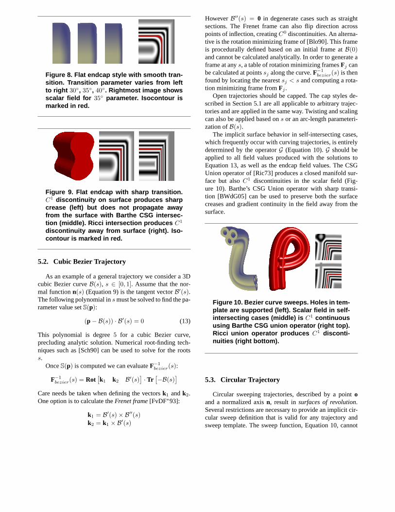
Figure 8. Flat endcap style with smooth tran-sition. Transition parameter varies from leftto right 30◦, 35◦, 40◦. Rightmost image showsscalar field for 35◦ parameter. Isocontour ismarked in red.

Figure 9. Flat endcap with sharp transition.C1 discontinuity on surface produces sharpcrease (left) but does not propagate awayfrom the surface with Barthe CSG intersec-tion (middle). Ricci intersection produces C1

discontinuity away from surface (right). Iso-contour is marked in red.

5.2. Cubic Bezier Trajectory

As an example of a general trajectory we consider a 3Dcubic Bezier curveB(s), s ∈ [0, 1]. Assume that the nor-mal functionn(s) (Equation 9) is the tangent vectorB′(s).The following polynomial ins must be solved to find the pa-rameter value setS(p):

(p − B(s)) · B′(s) = 0 (13)

This polynomial is degree5 for a cubic Bezier curve,precluding analytic solution. Numerical root-finding tech-niques such as [Sch90] can be used to solve for the rootss.

OnceS(p) is computed we can evaluateF−1

bezier(s):

F−1

bezier(s) = Rot[

k1 k2 B′(s)]

· Tr[

−B(s)]

Care needs be taken when defining the vectorsk1 andk2.One option is to calculate theFrenet frame[FvDF∗93]:

k1 = B′(s) × B′′(s)

k2 = k1 × B′(s)

HoweverB′′(s) = 0 in degenerate cases such as straightsections. The Frenet frame can also flip direction acrosspoints of inflection, creatingC0 discontinuities. An alterna-tive is the rotation minimizing frame of [Blo90]. This frameis procedurally defined based on an initial frame atB(0)and cannot be calculated analytically. In order to generateaframe at anys, a table of rotation minimizing framesFj canbe calculated at pointssj along the curve.F−1

bezier(s) is thenfound by locating the nearestsj < s and computing a rota-tion minimizing frame fromFj .

Open trajectories should be capped. The cap styles de-scribed in Section 5.1 are all applicable to arbitrary trajec-tories and are applied in the same way. Twisting and scalingcan also be applied based ons or an arc-length parameteri-zation ofB(s).

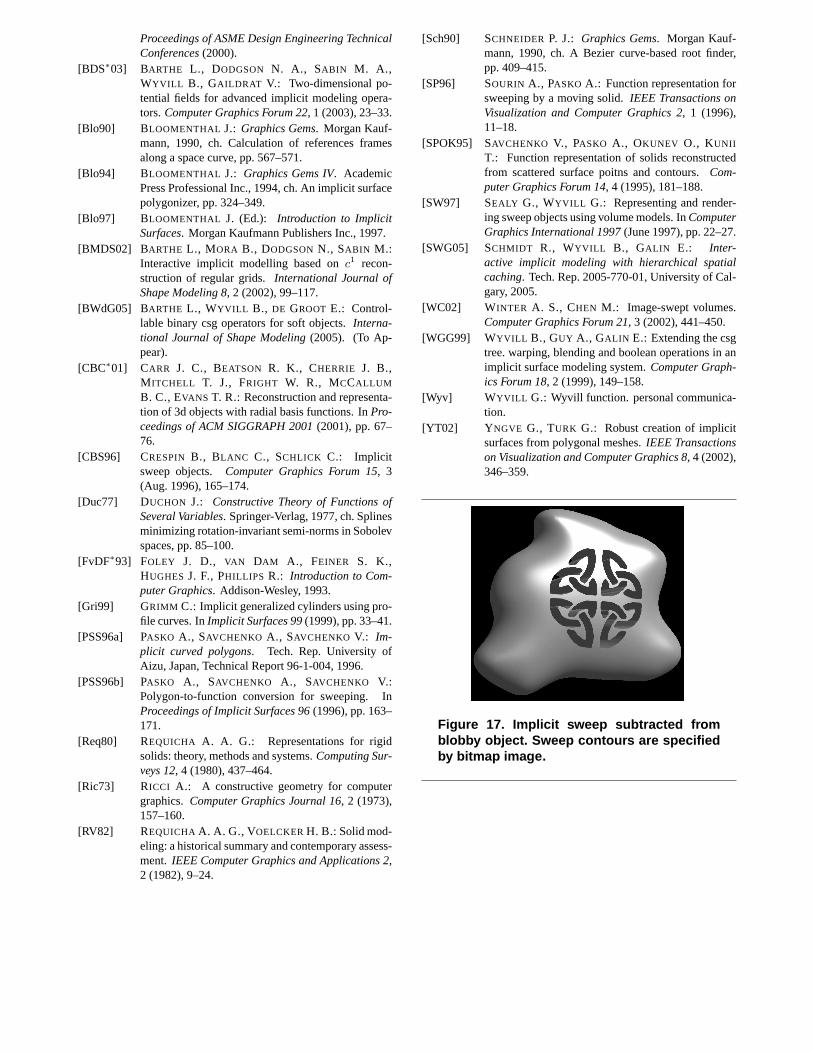
The implicit surface behavior in self-intersecting cases,which frequently occur with curving trajectories, is entirelydetermined by the operatorG (Equation 10).G should beapplied to all field values produced with the solutions toEquation 13, as well as the endcap field values. The CSGUnion operator of [Ric73] produces a closed manifold sur-face but alsoC1 discontinuities in the scalar field (Fig-ure 10). Barthe’s CSG Union operator with sharp transi-tion [BWdG05] can be used to preserve both the surfacecreases and gradient continuity in the field away from thesurface.

Figure 10. Bezier curve sweeps. Holes in tem-plate are supported (left). Scalar field in self-intersecting cases (middle) is C1 continuoususing Barthe CSG union operator (right top).Ricci union operator produces C1 disconti-nuities (right bottom).

5.3. Circular Trajectory

Circular sweeping trajectories, described by a pointoand a normalized axisn, result insurfaces of revolution.Several restrictions are necessary to provide an implicit cir-cular sweep definition that is valid for any trajectory andsweep template. The sweep function, Equation 10, cannot

be evaluated at points lying on the axisn because the setS(p) (Equation 9) is infinite. To define circular sweeps wemake a simplifying assumption - that the template orienta-tion and scaling is constant. Under this constraint the infi-nite parameter set maps to a single pointu.

Since we disallow twisting and scaling, it is possible tocompute pointu in the sweep template corresponding to apoint p without finding the angleθ on the circular trajec-tory. The 2D coordinates are found geometrically:

uy = (p − o) · nux = ‖(p − o) − uyn‖

The 2D coordinates corresponding to the opposingside of the circle are(−ux, uu). These sample points re-sult in two field values which we compose with theBarthe Union operator [BWdG05] to produce a gradient-continuous scalar field.

To support partial circular sweeps the parameterθmust be computed. The necessary equations can be foundin [WC02]. Our endcap techniques should be applied to par-tial sweeps to preventC0 discontinuity when the sweepterminates.

Figure 11. Invertible sweeps produce torus-like surfaces (a), while self-intersectingsweeps (b) are non-invertible because degen-erate points on n lie inside the field bounds.Geometric computation of 2D sweep tem-plate coordinates is shown in (c).

Note thatux ≥ 0, implying that the portion of the sweeptemplate to the left of the axis in Figure 11b is never sam-pled. This can be desirable as it is analogous to revolving anopen curve around an axis between the curve endpoints. Un-fortunately it also produces aC1 discontinuity at points onn wherefM is not continuousC1 continuous across theYaxis.

We also note that in certain cases (Figure 11a) field val-ues alongn are outside the bounds offM and therefore0.Here twisting can be safely applied, although for full circu-lar sweeps the twist angle needs be a whole multiple of2πto avoidC0 discontinuities. A similar limitation applies forscaling.

Figure 12. Circular trajectory sweep surfaces.

6. Applications

6.1. Interactive BlobTree modeling

The sweep primitives described in Section 5 can be useddirectly in implicit modeling systems such as theBlob-Tree [WGG99]. Sweep primitives implemented using thediscrete approximation technique of section 4.4 are very ef-ficient. We use them in an interactive BlobTree modelingtool.

A key limitation for interactive implicit modeling is vi-sualizing the current surface. We visualize BlobTree mod-els by generating a polygonal mesh that approximates thesurface [Blo94]. The main cost of polygonization is eval-uating the field function. Linear and circular sweeps canbe polygonized at resolutions adequate for modeling, pro-vided the sweep contour does not have very small fea-tures. Performance quickly degrades when composingseveral sweeps in a BlobTree. However, with hierarchi-cal spatial caching [SWG05] a large number of implicitsweep primitives can be manipulated interactively, in-cluding bezier curve sweeps. The models in Figures 13and 16 were all created using our interactive system.We note that zero-length linear sweeps with blobby end-caps are very useful for character modeling, as shown inFigure 16.

We note that while solving the linear system defined byEquation 5 isO(N3), the number of constraint points isusually less than one thousand. We use an SIMD-optimizedLAPACK implementation that solves these systems withdouble precision in a few seconds on a 1.6Ghz Pentium 4processor.

6.2. Parametric to Implicit sweep conversion

Many existing parametric modeling tools define sweepsurfaces using a boundary representation. In this case thesweep template is the contourC, usually defined para-metrically, and the sweep trajectory is a 3D parametriccurveT (s). The boundary representation has several lim-itations. Operations such as CSG, or even simple point-inclusion testing, require complex numerical techniques.

Figure 13. Implicit BlobTree models com-posed entirely of sweeps, blending, and CSG.Each model was created interactively in un-der 30 minutes.

Self-intersecting sweeps are difficult to handle [AMBJ00]because the definition of “inside” is ambiguous. Algorithmsfor measuring physical properties, such as volume, oftenproduce nonsense results in these degenerate cases.

Our implicit sweep representation easilyhandles degenerate conditions, CSG is well-supported [Ric73] [WGG99] [BWdG05], and point-inclusion testing is trivial using the implicit volume defin-ition (Equation 4). Conversion from parametric sweeps toour implicit sweeps is trivial, we simply re-use the para-metric contour contourC and trajectoryT (Section 5).

An important consideration when converting parametricsweeps to implicit sweeps is error introduced by the con-version. The 2D scalar field is produced using variationaltechniques that only approximateC (Section 4.3). However,by increasing the curve sampling rate when solving forfC(Section 4.2) the variational solution can be tightly con-strained. An example of parametric conversion is shown inFigure 14. In this case the maximum surface deviation isless than0.5%, which occurs at the high-curvature features.

Interactive tools for implicit modeling can take advan-tage of this coherence between parametric and implicitrepresentations. The sweep surface can be quickly visual-ized during interactive manipulation using parametric tech-niques. Once manipulation is complete, the implicit modelis re-polygonized.

6.3. Surface reconstruction from parallel contours

It is possible to interpolate between the two sweep tem-plate fieldsfM1

andfM2along a sweep with respect to a

Figure 14. Parametric sweep (left) and corre-sponding implicit sweep (middle). Parametricsweep vertices colored by implicit approxi-mation error (right). Error values have beenscaled by 1000.

parametert ∈ [0, 1]:

fMinterp(t) = (1 − t)fM1

+ (t)fM2

A sweep surface with varying cross section can be createdby sweeping the templatefMinterp

(s), where s is scaled to[0, 1]. The resulting surface smoothly transitions betweenthe two templates regardless of topology. Interpolation be-tweenn templates is accomplished by successively inter-polating between pairs of templates. Given a set of contoursCi, a closed surface can be reconstructed that passes throughall the contours.

A variety of techniques for implicit surface recon-struction from contours are available [SPOK95] [AG04][CBC∗01] [YT02]. One benefit of our approach is thatthe resulting field is very efficient to evaluate. In Fig-ure 15 a human L3 vertebra is reconstructed from 93segmented CT slices (See also Figure 18) . The recon-struction process takes approximately 6 minutes, howeveronce complete the implicit object (which is simply a lin-ear sweep) can be interactively edited in our BlobTreesystem

7. Conclusion

We have presented newC1 continuous implicit sweepobjects that have a bounded scalar field. Our sweep tem-plate fields can be generated from any set of closed 2D con-tours, including contours with “holes”. Implicit sweep ob-jects generated with our template fields are visually indis-tinguishable from triangle meshes created by sweeping thesame contour, even when using aC1 discrete approxima-tion to the 2D scalar field. Our endcap styles for open tra-jectories preserve field continuity, as do the CSG union op-erators applied for self-intersecting sweeps.

Figure 15. Surface reconstruction from con-tours. Human L3 vertebra is reconstructedfrom 93 slices (left) and interactively modifiedin a BlobTree modeling system (right). High-frequency ridges on vertebra surface are dueto manual segmentation errors.

These contributions permit direct specification and ma-nipulation of the implicit surface for a large class offree-form shapes. Direct surface interaction is desirableforshape modeling, but has not been available for implicit sur-faces with bounded fields. Bounded fields are necessary toachieve scalable interactive performance [SWG05] and pre-serve the “principle of least surprise” that is key for inter-active tools.

We have found that we rely on these sweep primitives al-most exclusively when using our interactive BlobTree mod-eling tool. However the traditional modeling interface isvery limited when working with complex hierarchical mod-els. One avenue for future research is the development ofnew interface metaphors and tools appropriate for interac-tive BlobTree modeling.

We have performed only very limited exploration intoparametric to implicit sweep conversion. Though the sur-face error in our tests was less than0.5%, this may stillbe outside of the acceptable tolerances for CAD/CAM ap-plications. A direction for future work would be to repre-sent the 2D contours exactly by integrating the functionalcurve representation of [PSS96a] with the improved opera-tors of [BDS∗03].

Finally, we have presented some basic results on surfacereconstruction from parallel contours. Implicit techniquesfor this problem have been previously developed. The ben-efit of our method is that the reconstructed model can be im-ported directly into our BlobTree modeling tool. This pro-vides another avenue to leverage existing models. The caseof medical data is particularly interesting - the interactiv-

ity afforded by our approach may have significant applica-tions in surgical training simulators.

Figure 16. Implicit BlobTree models com-posed mostly of zero-length linear sweepswith blobby endcaps. Top model also usesBezier sweep for nose and revolution for hat.

References

[AG04] AKKOUCHE S., GALIN E.: Implicit surface recon-struction from contours.The Visual Computer 20, 6(2004), 380–391.

[AMBJ00] ABDEL-MALEK K., BLACKMORE D., JOY K.:Swept volumes: Foundations, perspectives and appli-cations.submitted to International Journal of ShapeModeling(2000).

[AMYB00] A BDEL-MALEK K., YANG J., BLACKMORE D.:Closed-form swept volume of implicit surfaces. In

Proceedings of ASME Design Engineering TechnicalConferences(2000).

[BDS∗03] BARTHE L., DODGSON N. A., SABIN M. A.,WYVILL B., GAILDRAT V.: Two-dimensional po-tential fields for advanced implicit modeling opera-tors.Computer Graphics Forum 22, 1 (2003), 23–33.

[Blo90] BLOOMENTHAL J.: Graphics Gems. Morgan Kauf-mann, 1990, ch. Calculation of references framesalong a space curve, pp. 567–571.

[Blo94] BLOOMENTHAL J.: Graphics Gems IV. AcademicPress Professional Inc., 1994, ch. An implicit surfacepolygonizer, pp. 324–349.

[Blo97] BLOOMENTHAL J. (Ed.): Introduction to ImplicitSurfaces. Morgan Kaufmann Publishers Inc., 1997.

[BMDS02] BARTHE L., MORA B., DODGSON N., SABIN M.:Interactive implicit modelling based onc1 recon-struction of regular grids.International Journal ofShape Modeling 8, 2 (2002), 99–117.

[BWdG05] BARTHE L., WYVILL B., DE GROOT E.: Control-lable binary csg operators for soft objects.Interna-tional Journal of Shape Modeling(2005). (To Ap-pear).

[CBC∗01] CARR J. C., BEATSON R. K., CHERRIE J. B.,M ITCHELL T. J., FRIGHT W. R., MCCALLUM

B. C., EVANS T. R.: Reconstruction and representa-tion of 3d objects with radial basis functions. InPro-ceedings of ACM SIGGRAPH 2001(2001), pp. 67–76.

[CBS96] CRESPIN B., BLANC C., SCHLICK C.: Implicitsweep objects. Computer Graphics Forum 15, 3(Aug. 1996), 165–174.

[Duc77] DUCHON J.: Constructive Theory of Functions ofSeveral Variables. Springer-Verlag, 1977, ch. Splinesminimizing rotation-invariant semi-norms in Sobolevspaces, pp. 85–100.

[FvDF∗93] FOLEY J. D., VAN DAM A., FEINER S. K.,HUGHES J. F., PHILLIPS R.: Introduction to Com-puter Graphics. Addison-Wesley, 1993.

[Gri99] GRIMM C.: Implicit generalized cylinders using pro-file curves. InImplicit Surfaces 99(1999), pp. 33–41.

[PSS96a] PASKO A., SAVCHENKO A., SAVCHENKO V.: Im-plicit curved polygons. Tech. Rep. University ofAizu, Japan, Technical Report 96-1-004, 1996.

[PSS96b] PASKO A., SAVCHENKO A., SAVCHENKO V.:Polygon-to-function conversion for sweeping. InProceedings of Implicit Surfaces 96(1996), pp. 163–171.

[Req80] REQUICHA A. A. G.: Representations for rigidsolids: theory, methods and systems.Computing Sur-veys 12, 4 (1980), 437–464.

[Ric73] RICCI A.: A constructive geometry for computergraphics.Computer Graphics Journal 16, 2 (1973),157–160.

[RV82] REQUICHA A. A. G., VOELCKERH. B.: Solid mod-eling: a historical summary and contemporary assess-ment. IEEE Computer Graphics and Applications 2,2 (1982), 9–24.

[Sch90] SCHNEIDER P. J.: Graphics Gems. Morgan Kauf-mann, 1990, ch. A Bezier curve-based root finder,pp. 409–415.

[SP96] SOURIN A., PASKO A.: Function representation forsweeping by a moving solid.IEEE Transactions onVisualization and Computer Graphics 2, 1 (1996),11–18.

[SPOK95] SAVCHENKO V., PASKO A., OKUNEV O., KUNII

T.: Function representation of solids reconstructedfrom scattered surface poitns and contours.Com-puter Graphics Forum 14, 4 (1995), 181–188.

[SW97] SEALY G., WYVILL G.: Representing and render-ing sweep objects using volume models. InComputerGraphics International 1997(June 1997), pp. 22–27.

[SWG05] SCHMIDT R., WYVILL B., GALIN E.: Inter-active implicit modeling with hierarchical spatialcaching. Tech. Rep. 2005-770-01, University of Cal-gary, 2005.

[WC02] WINTER A. S., CHEN M.: Image-swept volumes.Computer Graphics Forum 21, 3 (2002), 441–450.

[WGG99] WYVILL B., GUY A., GALIN E.: Extending the csgtree. warping, blending and boolean operations in animplicit surface modeling system.Computer Graph-ics Forum 18, 2 (1999), 149–158.

[Wyv] W YVILL G.: Wyvill function. personal communica-tion.

[YT02] Y NGVE G., TURK G.: Robust creation of implicitsurfaces from polygonal meshes.IEEE Transactionson Visualization and Computer Graphics 8, 4 (2002),346–359.

Figure 17. Implicit sweep subtracted fromblobby object. Sweep contours are specifiedby bitmap image.

Figure 18. Various views of Human L3 Vertebra reconstructed by interpolating between planar im-plicit sweeps.