applied sciences

Article

Convergency and Stability of Explicit and Implicit Schemes inthe Simulation of the Heat Equation

Franyelit Suárez-Carreño 1,* and Luis Rosales-Romero 2

�����������������

Citation: Suárez-Carreño, F.;

Rosales-Romero, L. Convergency and

Stability of Explicit and Implicit

Schemes in the Simulation of the Heat

Equation. Appl. Sci. 2021, 11, 4468.

https://doi.org/10.3390/app11104468

Academic Editor: Filippo Berto

Received: 10 April 2021

Accepted: 27 April 2021

Published: 14 May 2021

Publisher’s Note: MDPI stays neutral

with regard to jurisdictional claims in

published maps and institutional affil-

iations.

Copyright: © 2021 by the authors.

Licensee MDPI, Basel, Switzerland.

This article is an open access article

distributed under the terms and

conditions of the Creative Commons

Attribution (CC BY) license (https://

creativecommons.org/licenses/by/

4.0/).

1 Industrial Engineering Career, Faculty of Engineering and Applied Sciences, University of the Americas,Quito 170902, Ecuador

2 Basic Science Department, Physics Section, Polytechnic University of Venezuela, UNEXPO,Puerto Ordaz 8050, Venezuela; lrosales@unexpo.edu.ve

* Correspondence: franyelit.suarez@udla.edu.ec

Featured Application: The authors show some computational highlights in the application of thesystem described above.

Abstract: Some strategies for solving differential equations based on the finite difference methodare presented: forward time centered space (FTSC), backward time centered space (BTSC), andthe Crank-Nicolson scheme (CN). These are developed and applied to a simple problem involvingthe one-dimensional (1D) (one spatial and one temporal dimension) heat equation in a thin bar.The numerical implementation in this work can be used as a preamble to introduce a method ofsolving the heat equation that can be implemented in problems in the area of finances. The resultsof implementing the software on very fine meshes (unidimensional), and with relatively small-time steps, are shown. Through mesh refinement, it was possible to obtain a better temperaturedistribution in the thin bar between a range of points. The heat equation was solved numericallyby testing both implicit (CN) and explicit (FTSC and BTSC) methods. The examples show that theimplemented schemes conform to theoretical predictions and that truncation errors depend on mesh,spacing, and time step.

Keywords: analytical solution; numerical methods; diffusion equation

1. Introduction

Most physical phenomena are represented by partial differential equations. Steady-state physical problems or time evolution problems are modeled through elliptic andparabolic partial differential equations, respectively; these equations are difficult to solveby analytical methods when the initial and boundary conditions are not simple. Anexample of this is shown in [1–3] and references therein, where several equations ofphysics-mathematics describing phenomena related to continuous element dynamics, elec-trodynamics, quantum mechanics, and mass and heat transfer phenomena are highlighted.For the solution of some of these equations, they use methods such as the Fourier Method,the Riemann Integration, and the use of the Green’s Function [4–8]. However, theseprocedures do not always guarantee analytical solutions that illustrate the behavior of amechanical system; this is where numerical methods provide powerful techniques thatallow a solution as close as possible to the reality of a specific problem.

The numerical methods developed by Harriot [9–15] were used to solve equationsand transcended in an important way to engineering in 1943 when Courant developed thefinite element method. Courant used the numerical methods of variation proposed by Ritzto obtain approximate solutions for mechanical systems [16,17]. The Courant–Friedrichs–Lewy (CFL) condition is a necessary condition for convergence in the numerical solutionof partial differential equations with partial differentials. A case of special importance iswhen time discretization schemes are used as a numerical solution. As a consequence, in

Appl. Sci. 2021, 11, 4468. https://doi.org/10.3390/app11104468 https://www.mdpi.com/journal/applsci

Appl. Sci. 2021, 11, 4468 2 of 16

many simulations, the time step has to be less than a characteristic value; otherwise, thecode may be unstable and not yield the correct results.

Thus, simulations are an effective tool in applied sciences to find solutions and predicttheir behavior. Additionally, they allow the mathematical recreation of physical processesthat frequently appear in engineering [18–20]. The use of simulations to study partialdifferential equations, in particular the diffusion equation, normally requires a carefulstudy of numerical methods, the algorithms to be used, and the fundamental processesto be included in the simulation. A simulation differs from a mathematical model in thatthe former is a representation at each instant of the process to be simulated, while themodel is a mathematical abstraction of the fundamental equations necessary to analyzethat phenomenon. Normally, the use of a simulation to study a given problem requirescareful planning of the mathematical model (partial differential equations and initialand boundary conditions) to be used and of the algorithms necessary to solve the model.Numerical methods are used to determine the numerical solution of problems for which theanalytical solution may or may not be known. These allow the translation of complicatedmathematical schemes using algorithms, the results of which can be contrasted with theanalytical solutions, in cases where such solutions exist.

In this work, the heat conduction equation is simulated to obtain the temperaturepatterns in a thin bar [21–23]. The analysis of non-stationary heat transfer is of practicalinterest, not only because of the importance that cooling and heating processes have in alarge number of industrial applications but also because of their similarity with severalother equations of physics-mathematics that present the same difficulties to be solvednumerically. Among the problems directly related to non-stationary heat transfer problemsare the starting and stopping of machines, processes that can lead, on the one hand, tothe appearance of important thermal loads on the solid with the consequent deterioration(turbine blades, for example), and on the other hand, to an increased emission of pollutingspecies (steam generators, gas turbines, and alternative internal combustion engines,among others).

For the reasons mentioned above, the efficient and accurate solution of the time-dependent differential equations of heat transfer plays a fundamental role, not only becauseof the number of engineering problems they represent but also as an initial or test case formany other more complex problems, in particular, the equations of fluid mechanics, whosecorrect solution depends on the efficiency shown by the different methods in the solutionof the heat transfer equations [1–3].

The increasing use of multiprocessor-based computers, either using parallel program-ming or multiple processors, has recently encouraged the use of explicit methods, which aremuch more apt to be parallelized due to their local information processing condition [4,5].It could be said that an explicit method, although more computationally expensive than animplicit method, is much more likely to be more efficient in parallel computation, and mayeven exceed it, depending on the number of parallel processors used [6–8].

In this work, we try to verify the results obtained previously, using implicit andexplicit methods that are stable for time steps much larger than those normally used in thistype of simulation with time dependence. The time steps achieved are, for similar accuracy,of the same order as those used in the implicit methods. In this way, all the advantagesconcerning the ease of parallel processing typical of the explicit ones are maintained withthe advantages of the implicit ones concerning their stability for large time steps [24,25].

N-soliton solutions could also be generated for (1 + 1)-dimensional integrable differ-ential equations; however, it is not of interest for this study to treat heat waves as solitons.The interest of this research is to test different discretization schemes in the solution ofpartial differential equations; to study the stability and convergence of each discretizationscheme in the one-dimensional heat diffusion equation; and, finally, to conclude whichscheme is more advantageous for future applications in various areas of interest.

Appl. Sci. 2021, 11, 4468 3 of 16

2. The Heat Equation

In engineering problems, it is common to find mathematical models that include par-tial differential equations [26–29]. The analytical solution provides a better understandingof the behavior of some phenomena since it can be determined at any instant of time. Ingeneral, it is not possible to determine this solution due to the non-linearity of the equationsthat constitute the mathematical model or due to the domain where the model is stud-ied. Numerical methods in science and engineering provide a tool that allows translatingmathematical models into computational procedures, whose results can be contrasted withthe analytical solutions, in those cases where they exist. In the following, an algorithmfor solving partial differential equations is shown, using the one-dimensional diffusionequation as a model problem. The choice of the same one is made based on its multipleapplications in problems of mechanics using the finite difference method to determine thenumerical solution of the diffusion equation using an explicit method and the implicit CNmethod [30,31].

The one-dimensional 1D heat equation is expressed by Equation (1)

∂∅∂t

= α∂2∅∂x2 0 ≤ x ≤ L, t ≥ 0 (1)

where ∅ = ∅(x, t) is the temperature and α is a constant coefficient. Equation (1) is amodel of transient heat conduction in a metallic segment of length L (physical domain).The material property α is the thermal diffusivity. In a practical calculation, the solution isobtained only for a finite time, tmax.

The solution to Equation (1) requires the specification of boundary conditions at x = 0and x = L, and initial conditions at t = 0. The initial and boundary conditions are [32,33]:

φ(0, t) = φ0, φ(L, t) = φL φ(x, 0) = ƒ0(x) (2)

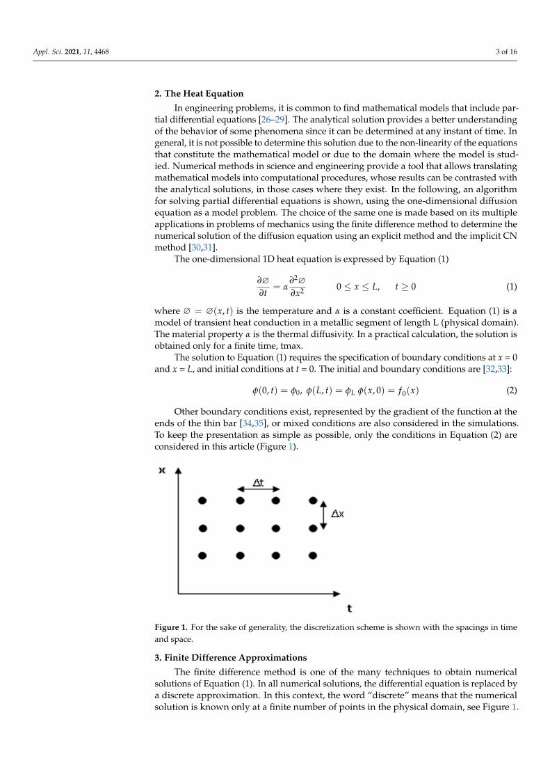
Other boundary conditions exist, represented by the gradient of the function at theends of the thin bar [34,35], or mixed conditions are also considered in the simulations.To keep the presentation as simple as possible, only the conditions in Equation (2) areconsidered in this article (Figure 1).

Figure 1. For the sake of generality, the discretization scheme is shown with the spacings in timeand space.

3. Finite Difference Approximations

The finite difference method is one of the many techniques to obtain numericalsolutions of Equation (1). In all numerical solutions, the differential equation is replaced bya discrete approximation. In this context, the word “discrete” means that the numericalsolution is known only at a finite number of points in the physical domain, see Figure 1.

Appl. Sci. 2021, 11, 4468 4 of 16

In general, increasing the number of points not only increases the resolution but also theaccuracy of the numerical solution [36,37].

In many cases, it is not possible to find an analytical solution, especially with those realphysical problems that have regions with non-regular geometry. However, convergenceand stability tests ensure that the finite difference approximations used in the discretizationare correct. There are ways to calculate the convergence of a code when the analyticalsolutions are known. Here, the parameters are taken into account to have a sufficiently finemesh and thus obtain a convergent system in as few iterations as possible. To this end, weresort to the condition ∆x ≤ k ∆t, to ensure that the meshing is the one that best fits thesolution space to be discretized. Knowing the value of ∆x, the minimum number of nodesto give a numerical solution to this system can be determined. In this way, the central ideaof the finite difference method is to replace continuous derivatives with so-called differenceformulas involving only the discrete values associated with positions on the grid.

Applying the finite difference method to a differential equation involves replacing thederivatives with the corresponding finite difference expression, according to the appro-priate scheme and accuracy. In the heat equation, there are derivatives concerning timeand derivatives concerning space. Using different grids should confirm the stability of thesolutions. In the limit when the mesh spacing (∆x and ∆t) tends to zero, the numericalsolution with either scheme will approach the true solution to the original differential equa-tion, or the numerical solution approaches with less error to the true solution. However,how close the numerical solution approaches the true solution varies with the differencescheme used. Additionally, some practically useful schemes may fail to give a solution forbad combinations of ∆x and ∆t. This is what we want to verify in this work [38].

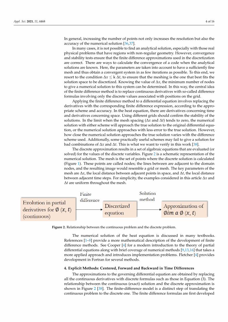
The discrete approximation results in a set of algebraic equations that are evaluated (orsolved) for the values of the discrete variables. Figure 2 is a schematic representation of thenumerical solution. The mesh is the set of points where the discrete solution is calculated(Figure 1). These points are called nodes; the lines between are adjacent to the domainnodes, and the resulting image would resemble a grid or mesh. The key parameters of themesh are ∆x, the local distance between adjacent points in space, and ∆t, the local distancebetween adjacent time steps. For simplicity, the examples considered in this article ∆x and∆t are uniform throughout the mesh.

Figure 2. Relationship between the continuous problem and the discrete problem.

The numerical solution of the heat equation is discussed in many textbooks.References [1–8] provide a more mathematical description of the development of finitedifference methods. See Cooper [4] for a modern introduction to the theory of partialdifferential equations along with brief coverage of numerical methods [9,13,16] that takes amore applied approach and introduces implementation problems. Fletcher [4] providesdevelopment in Fortran for several methods.

4. Explicit Methods: Centered, Forward and Backward in Time Differences

The approximations to the governing differential equation are obtained by replacingall the continuous derivatives with discrete formulas such as those in Equation (3). Therelationship between the continuous (exact) solution and the discrete approximation isshown in Figure 2 [38]. The finite-difference model is a distinct step of translating thecontinuous problem to the discrete one. The finite difference formulas are first developed

Appl. Sci. 2021, 11, 4468 5 of 16

with the dependent variable Ø as a function of a single independent variable, x, i.e.,∅ = ∅(x). The resulting formulas are then used to approximate derivatives concerningany space or time.

4.1. Direct Finite Difference of First Order

Consider a Taylor series expansion φ (x) over the point.

φ (xi + δx) = ∅(xi) + δx (3)

φ (x) first order direct difference. Consider a Taylor series expansion φ (x) over the point

φ(xi + δx) = φ(xi) + δx∂φ

∂x

∣∣∣∣xi +δx2

2∂2φ

∂x2

∣∣∣∣xi +δx3

3!∂3φ

∂x3

∣∣∣∣xi + . . . (4)

where δx is a change in x to relative to xi. Let δx = ∆x in Equation (4), that is, considerthe value ∅ at the location of the mesh line xi + 1, i.e., ∅(xi + ∆x) = ∅(xi) + ∆x Note thatthe powers of multiply partial derivatives to the right-hand side have been reduced byone. The approximate solution is replaced by the exact solution, i.e., using ∅i ≈ ∅(xi)y ∅i + 1 ≈ ∅(xi + ∆x)

∂φ

∂x

∣∣∣∣xi ≈φi+1 − φi

∆x− ∆x

2∂2φ

∂x2

∣∣∣∣xi −∆x3

3!∂3φ

∂x3

∣∣∣∣xi + . . . (5)

The mean value theorem can be used to replace the higher-order derivatives

∂φ

∂x

∣∣∣∣xi ≈φi+1 − φi

∆x+

∆x2

2∂2φ

∂x2

∣∣∣∣ε

or∂φ

∂x

∣∣∣∣xi −φi+1 − φi

∆x≈ ∆x2

2∂2φ

∂x2

∣∣∣∣ε

(6)

The term on the right-hand side of Equation (6) is called the truncation of the fi-nite difference approximation. It is the error that results from truncating the series inEquation (5). In general, ξ is not known and is determined from the simulation. Althoughin the exact magnitude the truncation error cannot be known (unless the true solution Ø(x, t) is known analytically). The notation “O” can be used to express the dependence ofthe truncation error on the mesh spacing. The right-hand side of Equation (6) contains themesh spacing ∆x, which is selected for convenience.

The equal sign in this expression is true in the order of magnitude sense. That is, theO = ∆x2 on the right-hand side of the expression is not strictly equal. Rather, the expressionmeans that the left-hand side is a product of an unknown constant and ∆x2. Althoughthe expression does not give the exact magnitude of the error, it tells us how fast thatterm approaches zero as ∆x becomes smaller. Using the notation O large, one can writeEquation (5) as

∂φ

∂x

∣∣∣∣xi =φi+1 − φi

∆x+ O(∆x) (7)

The Equation (7) is known as the forward difference formula for(

∂∅∂x

)xi because it

involves xi and xi+1 nodes. The forward difference approximation has a truncation errorthat is O (∆x). The size of the truncation error is under control because the mesh size ∆xcan be chosen.

Appl. Sci. 2021, 11, 4468 6 of 16

4.1.1. First-Order Backward Difference

An alternative first-order finite difference formula is obtained if the Taylor series thusin Equation (4) is written with δx = −∆x. Using the discrete variable mesh instead of allunknowns, one obtains

∂∅∂x

∣∣∣∣xi =φi − φi+1

∆x+ O(∆x) (8a)

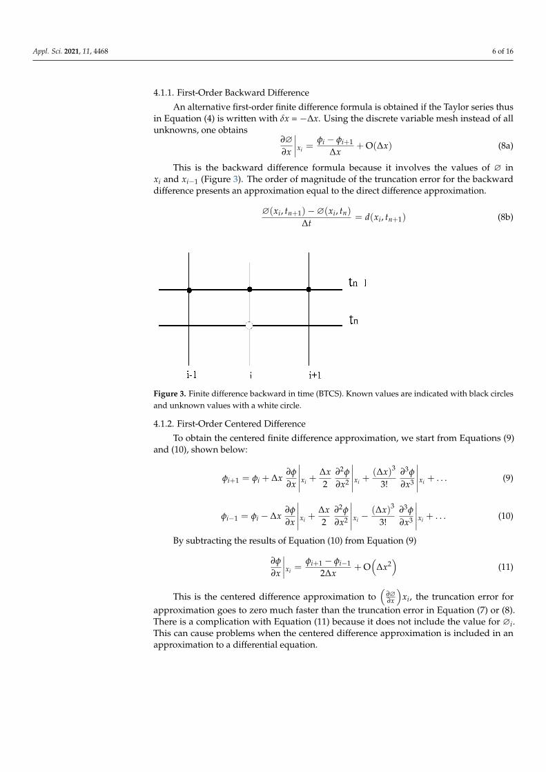
This is the backward difference formula because it involves the values of ∅ inxi and xi−1 (Figure 3). The order of magnitude of the truncation error for the backwarddifference presents an approximation equal to the direct difference approximation.

∅(xi, tn+1)−∅(xi, tn)

∆t= d(xi, tn+1) (8b)

Figure 3. Finite difference backward in time (BTCS). Known values are indicated with black circlesand unknown values with a white circle.

4.1.2. First-Order Centered Difference

To obtain the centered finite difference approximation, we start from Equations (9)and (10), shown below:

φi+1 = φi + ∆x∂φ

∂x

∣∣∣∣∣xi +∆x2

∂2φ

∂x2

∣∣∣∣∣xi +(∆x)3

3!∂3φ

∂x3

∣∣∣∣∣xi + . . . (9)

φi−1 = φi − ∆x∂φ

∂x

∣∣∣∣∣xi +∆x2

∂2φ

∂x2

∣∣∣∣∣xi −(∆x)3

3!∂3φ

∂x3

∣∣∣∣∣xi + . . . (10)

By subtracting the results of Equation (10) from Equation (9)

∂φ

∂x

∣∣∣∣xi =φi+1 − φi−1

2∆x+ O

(∆x2

)(11)

This is the centered difference approximation to(

∂∅∂x

)xi, the truncation error for

approximation goes to zero much faster than the truncation error in Equation (7) or (8).There is a complication with Equation (11) because it does not include the value for ∅i.This can cause problems when the centered difference approximation is included in anapproximation to a differential equation.

Appl. Sci. 2021, 11, 4468 7 of 16

4.1.3. Second-Order Centered Difference

Finite difference approximations to higher order derivatives can be obtained with theadditional manipulations of the Taylor series expansion over ∅(xi). Adding the yields ofEquations (9) and (10).

∂2φ

∂x2

∣∣∣∣xi =φi+1 − 2φi + φi+1

∆ x2 + O(

∆x2)

(12)

This is also called the central difference approximation, but (obviously) it is theapproximation to the second derivative, while Equation (11) is the central differenceapproximation to the first derivative.

The finite-difference approximations developed above are now assembled into adiscrete approximation to Equation (1). Both time and spatial derivatives are replaced byfinite differences. Doing so requires specification of both the time and spatial locations ofthe Ø values in the finite-difference. Therefore, one needs to introduce the superscript m todesignate the time of the discrete solution step. Although this seems to be only a simpleproblem, choosing the time step where the spatial derivatives are evaluated will have agreat impact on the convergence and stability of finite difference implementation.

4.1.4. Difference Centered Forward in Time

Approximates the derivative of time in Equation (1) with a direct difference

∂φ

∂t

∣∣∣∣∣tm+1, xi =φn+1

i − φni

∆t+ O(∆x) (13)

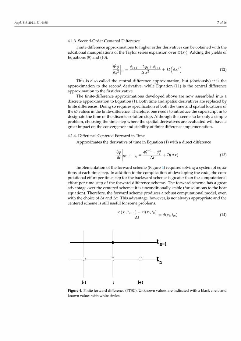
Implementation of the forward scheme (Figure 4) requires solving a system of equa-tions at each time step. In addition to the complication of developing the code, the com-putational effort per time step for the backward scheme is greater than the computationaleffort per time step of the forward difference scheme. The forward scheme has a greatadvantage over the centered scheme: it is unconditionally stable (for solutions to the heatequation). Therefore, the forward scheme produces a robust computational model, evenwith the choice of ∆t and ∆x. This advantage, however, is not always appropriate and thecentered scheme is still useful for some problems.

∅(xi, tn+1)−∅(xi, tn)

∆t= d(xi, tm) (14)

Figure 4. Finite forward difference (FTSC). Unknown values are indicated with a black circle andknown values with white circles.

Appl. Sci. 2021, 11, 4468 8 of 16

4.1.5. Implicit Method: Crank-Nicolson (CN)

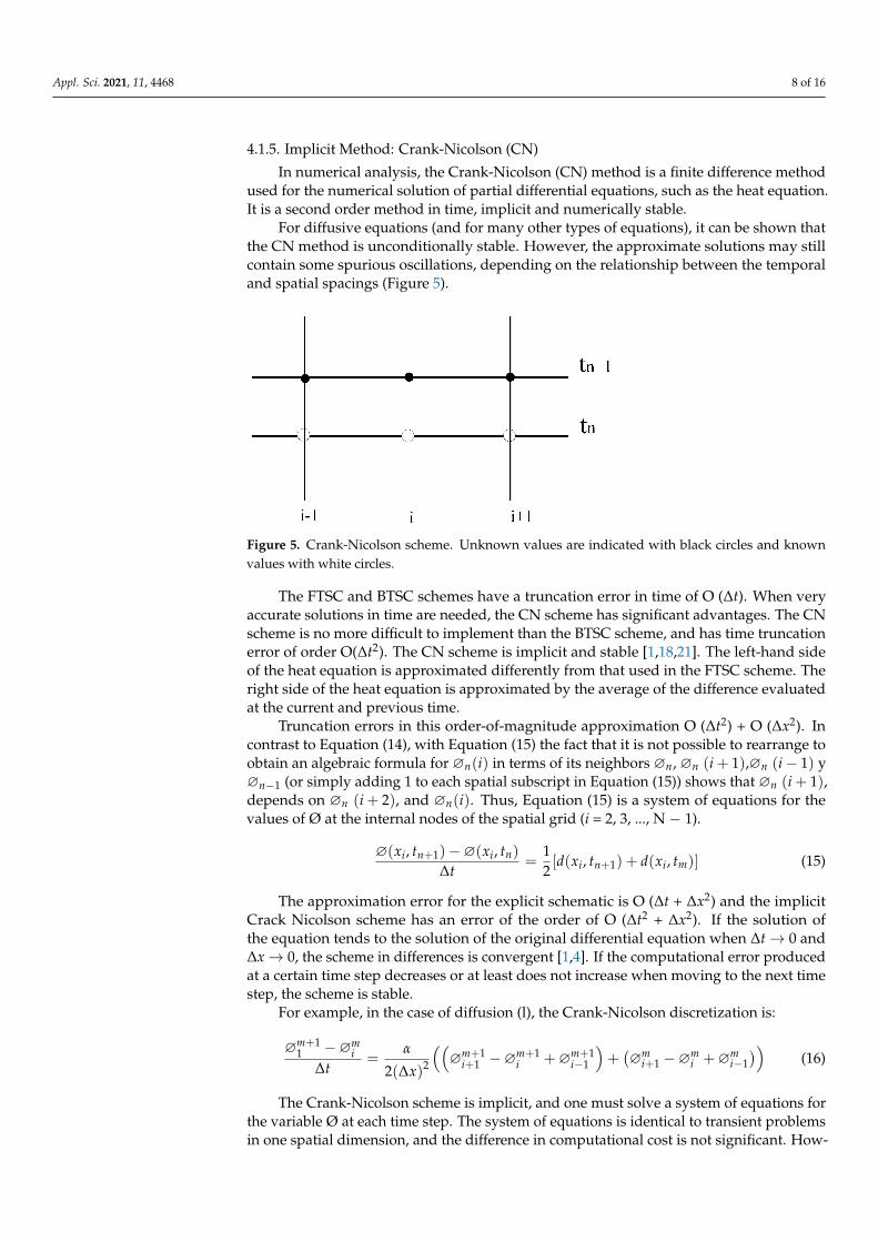
In numerical analysis, the Crank-Nicolson (CN) method is a finite difference methodused for the numerical solution of partial differential equations, such as the heat equation.It is a second order method in time, implicit and numerically stable.

For diffusive equations (and for many other types of equations), it can be shown thatthe CN method is unconditionally stable. However, the approximate solutions may stillcontain some spurious oscillations, depending on the relationship between the temporaland spatial spacings (Figure 5).

Figure 5. Crank-Nicolson scheme. Unknown values are indicated with black circles and knownvalues with white circles.

The FTSC and BTSC schemes have a truncation error in time of O (∆t). When veryaccurate solutions in time are needed, the CN scheme has significant advantages. The CNscheme is no more difficult to implement than the BTSC scheme, and has time truncationerror of order O(∆t2). The CN scheme is implicit and stable [1,18,21]. The left-hand sideof the heat equation is approximated differently from that used in the FTSC scheme. Theright side of the heat equation is approximated by the average of the difference evaluatedat the current and previous time.

Truncation errors in this order-of-magnitude approximation O (∆t2) + O (∆x2). Incontrast to Equation (14), with Equation (15) the fact that it is not possible to rearrange toobtain an algebraic formula for ∅n(i) in terms of its neighbors ∅n, ∅n (i + 1),∅n (i− 1) y∅n−1 (or simply adding 1 to each spatial subscript in Equation (15)) shows that ∅n (i + 1),depends on ∅n (i + 2), and ∅n(i). Thus, Equation (15) is a system of equations for thevalues of Ø at the internal nodes of the spatial grid (i = 2, 3, ..., N − 1).

∅(xi, tn+1)−∅(xi, tn)

∆t=

12[d(xi, tn+1) + d(xi, tm)] (15)

The approximation error for the explicit schematic is O (∆t + ∆x2) and the implicitCrack Nicolson scheme has an error of the order of O (∆t2 + ∆x2). If the solution ofthe equation tends to the solution of the original differential equation when ∆t→ 0 and∆x→ 0, the scheme in differences is convergent [1,4]. If the computational error producedat a certain time step decreases or at least does not increase when moving to the next timestep, the scheme is stable.

For example, in the case of diffusion (l), the Crank-Nicolson discretization is:

∅m+11 −∅m

i∆t

=α

2(∆x)2

((∅m+1

i+1 −∅m+1i +∅m+1

i−1

)+(∅m

i+1 −∅mi +∅m

i−1))

(16)

The Crank-Nicolson scheme is implicit, and one must solve a system of equations forthe variable Ø at each time step. The system of equations is identical to transient problemsin one spatial dimension, and the difference in computational cost is not significant. How-

Appl. Sci. 2021, 11, 4468 9 of 16

ever, for transient problems with two or three spatial dimensions, the computational effortper forward time step is much larger than the computational effort per centered time stepof difference. However, the stability is higher than forward. In problems in one, two, orthree dimensions, CN generally provides a computational advantage [38].

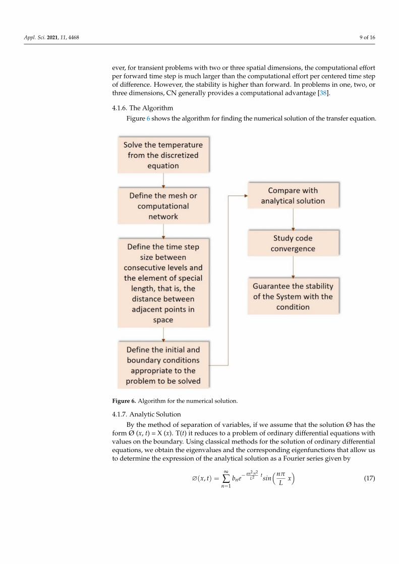
4.1.6. The Algorithm

Figure 6 shows the algorithm for finding the numerical solution of the transfer equation.

Figure 6. Algorithm for the numerical solution.

4.1.7. Analytic Solution

By the method of separation of variables, if we assume that the solution Ø has theform Ø (x, t) = X (x). T(t) it reduces to a problem of ordinary differential equations withvalues on the boundary. Using classical methods for the solution of ordinary differentialequations, we obtain the eigenvalues and the corresponding eigenfunctions that allow usto determine the expression of the analytical solution as a Fourier series given by

∅(x, t) =∞

∑n=1

bne−an2π2

L2 tsin(nπ

Lx)

(17)

Appl. Sci. 2021, 11, 4468 10 of 16

where bn with n ∈ N are the coefficients of the Fourier series development of the functionf (x) (initial condition of the problem) and are determined by the formula

bn =2L

L∫0

f (x)sin(nπ

Lx)

dx (18)

With the appropriate boundary conditions the analytical solution Ø (x, t) is ob-tained [39,40].

5. Results5.1. Numerical Implementation

The finite difference method allows us to obtain an approximate solution for Ø (x, t)at a finite set of points x and t for the codes developed in this paper. There are plausibleschemes that do not exhibit this important property of converging to the true solution. Seethe consistency discussions in references [1,4]. The numerical implementation is performeduniformly spaced in the interval 0 ≤ x ≤ L such that xi = (i− 1)∆x, i = 1, 2, 3 . . . N whereis the total number of spatial nodes, including those on the edge. Given L and N, the spacebetween xi is calculated with ∆x = L/(N − 1). Similarly, the discrete times are uniformlyspaced in 0 ≤ t ≤ tmax : tm = (m− 1)∆t, m = 1, 2, ..M where M is the maximum numberof time steps and ∆t is the size of a time step ∆t = tmax/(M− 1).

5.2. Estimates of Truncation Error (TE)

The TE for the centered or forward schemes is O (∆t) + O (∆x2). The notation O largeexpresses the rate at which the TE reaches zero. For code validation, we worked with themagnitude of the TE. For a ∆t, ∆x given as ∆t→ 0 and ∆t→ 0, the true magnitude of thetruncation error is [41–46]

TE = Kt∆t + Kx∆x2 (19)

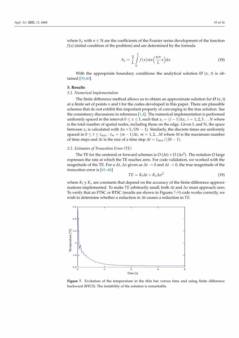
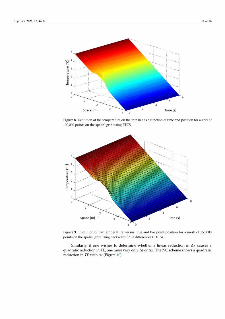
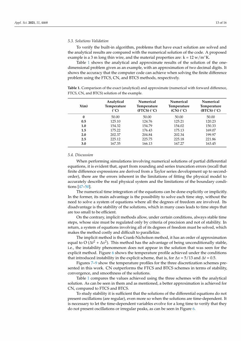
where Kt y Kx are constants that depend on the accuracy of the finite-difference approxi-mations implemented. To make TE arbitrarily small, both ∆t and ∆x must approach zero.To verify that an FTSC or BTSC (results are shown in Figures 7–9) code works correctly, wewish to determine whether a reduction in ∆t causes a reduction in TE.

Figure 7. Evolution of the temperature in the thin bar versus time and using finite differencebackward (BTCS). The instability of the solution is remarkable.

Appl. Sci. 2021, 11, 4468 11 of 16

Figure 8. Evolution of the temperature on the thin bar as a function of time and position for a grid of100,000 points on the spatial grid using FTCS.

Figure 9. Evolution of bar temperature versus time and bar point position for a mesh of 150,000points on the spatial grid using backward finite differences (BTCS).

Similarly, if one wishes to determine whether a linear reduction in ∆x causes aquadratic reduction in TE, one must vary only ∆t or ∆x. The NC scheme shows a quadraticreduction in TE with ∆t (Figure 10).

Appl. Sci. 2021, 11, 4468 12 of 16

Figure 10. Evolution of bar temperature versus time and bar point position for a mesh of 150,000points on the spatial grid using Crank-Nicolson (CN).

One could also use the second-order L1 rules norm, comparing the numerical solutionwith the analytical one to determine the error at the level of approximation, as expected.

Figure 11 shows the pseudocode used for the analysis of the heat equation.

Figure 11. Pseudo code showing the numerical scheme in FORTRAN 77 implemented with finitedifference for the heat equation.

Appl. Sci. 2021, 11, 4468 13 of 16

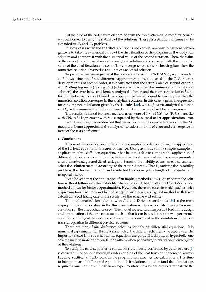
5.3. Solutions Validation

To verify the built-in algorithm, problems that have exact solution are solved andthe analytical results are compared with the numerical solution of the code. A proposedexample is a 3 m long thin wire, and the material properties are: k = 12 w/m◦K.

Table 1 shows the analytical and approximate results of the solution of the one-dimensional problem given as an example, with an approximation of two decimal digits. Itshows the accuracy that the computer code can achieve when solving the finite differenceproblem using the FTCS, CN, and BTCS methods, respectively.

Table 1. Comparison of the exact (analytical) and approximate (numerical with forward difference,FTCS, CN, and BTCS) solution of the example.

X(m)Analytical

Temperature(◦C)

NumericalTemperature(FTCS) (◦C)

NumericalTemperature

(CN) (◦C)

NumericalTemperature(BTCS) (◦C)

0 50.00 50.00 50.00 50.000.5 125.10 124.76 125.21 120.231.0 154.32 154.79 154.02 150.331.5 175.22 176.43 175.13 169.072.0 202.37 204.84 202.34 199.972.5 225.12 225.75 225.18 221.863.0 167.35 166.13 167.27 163.45

5.4. Discussion

When performing simulations involving numerical solutions of partial differentialequations, it is evident that, apart from rounding and series truncation errors (recall thatfinite difference expressions are derived from a Taylor series development up to second-order), there are the errors inherent in the limitations of fitting the physical model toaccurately describe the real physical system and the limitations of the boundary condi-tions [47–50].

The numerical time integration of the equations can be done explicitly or implicitly.In the former, its main advantage is the possibility to solve each time step, without theneed to solve a system of equations where all the degrees of freedom are involved. Itsdisadvantage is the stability of the solutions, which in many cases leads to time steps thatare too small to be efficient.

On the contrary, implicit methods allow, under certain conditions, always stable timesteps, whose size must be regulated only by criteria of precision and not of stability. Inreturn, a system of equations involving all of its degrees of freedom must be solved, whichmakes the method costly and difficult to parallelize.

The implicit method is the Crank-Nicholson method, it has an order of approximationequal to O (∆t2 + ∆x2). This method has the advantage of being unconditionally stable,i.e., the instability phenomenon does not appear in the solution that was seen for theexplicit method. Figure 6 shows the temperature profile achieved under the conditionsthat introduced instability in the explicit scheme, that is, for ∆x = 5/13 and ∆t = 0.5.

Figures 7–9 show the temperature profiles for the three discretization schemes pre-sented in this work. CN outperforms the FTCS and BTCS schemes in terms of stability,convergence, and smoothness of the solutions.

Table 1 compares the values achieved using the three schemes with the analyticalsolution. As can be seen in them and as mentioned, a better approximation is achieved forCN, compared to FTCS and BTCS.

To study stability it is sufficient that the solutions of the differential equations do notpresent oscillations (are regular), even more so when the solutions are time-dependent. Itis necessary to let the time-dependent variables evolve for a long time to verify that theydo not present oscillations or irregular peaks, as can be seen in Figure 6.

Appl. Sci. 2021, 11, 4468 14 of 16

All the runs of the codes were elaborated with the three schemes. A mesh refinementwas performed to verify the stability of the solutions. These discretization schemes can beextended to 2D and 3D problems.

In some cases when the analytical solution is not known, one way to perform conver-gence is to take the numerical value of the first iteration of the program as the analyticalsolution and compare it with the numerical value of the second iteration. Then, the valueof the second iteration is taken as the analytical solution and compared with the numericalvalue of the third iteration and so on. The convergence consists of checking how close thenumerical solution obtained is to a known analytical solution.

To perform the convergence of the code elaborated in FORTRAN77, we proceededas follows: since the finite difference approximation method used in the Taylor seriesdevelopment is of second order, it is postulated that the error is also of second order in∆x. Plotting log (error) Vs log (∆x) (where error involves the numerical and analyticalsolution), the error between a known analytical solution and the numerical solution foundfor the heat equation is obtained. A slope approximately equal to two implies that thenumerical solution converges to the analytical solution. In this case, a general expressionfor convergence calculation given by the L1 rules [20], where fij is the analytical solutionand Fij is the numerical solution obtained and L1 = Error, was used for convergence.

The results obtained for each method used were of 1.7 (BTCS), 1.8 (FTCS), and 2.0with CN, in full agreement with those expected by the second-order approximation error.

From the above, it is established that the errors found showed a tendency for the NCmethod to better approximate the analytical solution in terms of error and convergence inmost of the tests performed.

6. Conclusions

This work serves as a preamble to more complex problems such as the applicationof the 1D heat equation in the area of finance. Using as motivation a simple example ofapplication of the diffusion equation, it has been possible to compare the application ofdifferent methods for its solution. Explicit and implicit numerical methods were presentedwith their advantages and disadvantages in terms of the stability of each one. The user canselect the solution method according to the required needs. That is, noticing the instabilityproblem, the desired method can be selected by choosing the length of the spatial andtemporal interval.

It can be seen that the application of an implicit method allows one to obtain the solu-tion without falling into the instability phenomenon. Additionally, the Crank-Nicholsonmethod allows for better approximation. However, there are cases in which such a strictapproximation error may not be necessary; in such cases, an explicit method with fewercalculations but taking care of the stability of the scheme will suffice.

The mathematical formulation with CN and Dirichlet conditions [34] is the mostappropriate for the solution in the three cases shown. This was verified using Newmanconditions in the three schemes used. This model represents an important tool in the designand optimization of the processes, so much so that it can be used to test new experimentalconditions, aiming at the decrease of time and costs involved in the simulation of the heattransfer equation in different physical systems.

There are many finite difference schemes for solving differential equations. It isnumerical experimentation that reveals which of the different schemes is the best to use. Theimportant factor is to see whether the equations are parabolic, elliptic, or hyperbolic; onescheme may be more appropriate than others when performing stability and convergenceof the solutions.

To verify the results, a series of simulations previously performed by other authors [1]is carried out to induce a thorough understanding of the heat transfer phenomena, alwayskeeping a critical attitude towards the program that executes the calculations. It is timeto integrate partial differential equations and simulations to understand that simulationsrequire as much or more time than an experimentalist in a laboratory to demonstrate the

Appl. Sci. 2021, 11, 4468 15 of 16

veracity, validity, and strengths of the same and contribute to establishing the paradigmsof all the aspects that accompany a simulation. All the cases were solved with FORTRAN77. In several cases, the capabilities of the program developed with FORTRAN 77 werereached in terms of meshes and calculation times.

Author Contributions: Conceptualization, F.S.-C. and L.R.-R.; methodology, F.S.-C. and L.R.-R.;investigation, F.S.-C. and L.R.-R.; writing—original draft preparation L.R-R.; writing—review andediting F.S.-C.; supervision, F.S.-C. and L.R.-R.; project administration, F.S.-C. and L.R.-R. Bothauthors have read and agreed to the published version of the manuscript.

Funding: This research was funded by Universidad de Las Américas-Ecuador and UniversidadPolitécnica de Venezuela, Puerto Ordaz.

Institutional Review Board Statement: Not applicable.

Informed Consent Statement: Not applicable.

Data Availability Statement: The data has not been published in any other journal or any other placeof publication. However, they are available at the UNEXPO Physics Laboratory,Puerto Ordaz, Venezuela.

Conflicts of Interest: The authors declare no conflict of interest.

References1. Ames, W. Numerical Methods for Partial Differential Equations; Academic Press, Inc.: Boston, MA, USA, 1992.2. Olsen-Kettle, L. Numerical Solution of Partial Differential Equations and Code; Swinburne University of Technology: Melbourne,

Australia, 2011; pp. 14–28.3. Adak, M. Comparison of Explicit and Implicit Finite Difference Schemes on Diffusion Equation. In Mathematical Modeling and

Computational Tools ICACM 2018. Springer Proceedings in Mathematics & Statistics; Bhattacharyya, S., Kumar, J., Ghoshal, K., Eds.;Springer: Singapore, 2018; Volume 320.

4. Cooper, J. Introductin to Partial Differential Equations with Matlab; Birkhuser: Boston, MA, USA, 1998.5. Sequeira-Chavarría, F.; Ramírez-Bogantes, M. Computational Aspects of the Finite Difference Method for the Time-Dependent

Heat Equation. Uniciencia 2019, 33, 83–100. [CrossRef]6. Morton, K.W.; Mayers, D.F. Numerical Solution of Partial Differential Equations: An Introduction; Cambridge University Press:

Cambridge, UK, 1994.7. Chapra, S.C.; Canale, R.P. Métodos Numéricos Para Ingenieros; McGraw-Hill/Interamericana Editores: New York, NY, USA, 2007.8. Millán, Z.; de la Torre, L.; Oliva, L.; Berenguer, M. Simulación numérica: Ecuación de difusión. Rev. Iberoam. Ing. Mecánica 2011,

15, 29–38.9. Fletcher, C. Computational Techniquess for Fluid Dynamics; Springer: Berlin, Germany, 1998.10. Khan, M.N.; Ahmad, I.; Akgül, A.; Ahmad, H.; Thounthong, P. Numerical solution of time-fractional coupled Korteweg–de Vries

and Klein–Gordon equations by local meshless method. Pramana J. Phys. 2021, 95, 6. [CrossRef]11. Liu, C.; Liu, X.; Yang, Z.; Yang, H.; Huang, J. New stability results of generalized impulsive functional differential equations. Sci.

China Inf. Sci. 2021, 65, 129201(2022). [CrossRef]12. Recktenwald, G. Finite-Difference Approximations to the Heat Equation. Mech. Eng. 2011, 10, 4–20.13. Golub, G.; Ortega, J. Scientific Computing: An Introduction with Parallel Computing; Academic Press, Inc.: Boston, UK, 1993.14. Camacho, A.; Guardian, B.; Jacobo, V.; Ortiz, A. El método alternativo de Schwarz y la computación paralela. In Proceedings of

the MEMORIAS XXIV Congreso Internacional Anual de la SOMIM, Campeche, Mexico, 19–21 September 2018; pp. 77–82.15. Huang, J.; Nualart, D.; Viitasaari, L. A central limit theorem for the stochastic heat equation. Stoch. Process. Appl. 2020, 130,

7170–7184. [CrossRef]16. Hoffman, J. Numerical Methods for Engineers and Scientists; McGraw-Hill: New York, NY, USA, 1992.17. O’Neil, P. Matemáticas Avanzadas Para Ingeniería, 7th ed.; Cengage Learning: Boston, MA, USA, 2015.18. Ibarra, M.C. La ecuación de calor de Fourier: Resolución mediante métodos de análisis en variable real y en variable compleja.

In UTN Facultad Regional Resistencia: II Jornadas de Investigación en Ingeniería del NEA y Países Limítrofes; Universidad TécnicaNacional: Misiones, Argentina, 2012.

19. Mamani Condori, F.; Gonzales Medina, R. Aplicación de Las Series de Fourier en la Solución de Problemas Con Valor Inicial en laFrontera. Veritas 2019, 13, 225–230.

20. Cranmer, K.; Brehmer, J.; Louppe, G. The frontier of simulation-based inference. Proc. Natl. Acad. Sci. USA 2020, 117, 30055–30062.[CrossRef]

21. Cannon, J. The One-Dimensional Heat Equation, Encyclopedia of Mathematics and Its Applications; Cambridge University Press:Cambridge, UK, 1984.

Appl. Sci. 2021, 11, 4468 16 of 16

22. Martín-Vaquero, J.; Vigo-Aguiar, J. On the numerical solution of the heat conduction equations subject to nonlocal conditions.Appl. Numer. Math. 2009, 59, 2507–2514. [CrossRef]

23. Li, Y. Central limit theorem for a fractional stochastic heat equation with spatially correlated noise. Adv. Differ. Equ. 2020, 1–9.[CrossRef]

24. Madera, S.; Ortega-Quitana, F.; Lopez, A.; Perez, O. Determinación del Coeficiente Convectivo de Transferencia de Calor delProceso de Escaldado de Zapallo (Cucurbita maxima). Inf. Tecnol. 2017, 28, 59–66. [CrossRef]

25. Meza Castro, I.F.; Herrera Acuña, A.E.; Obregón Quiñones, L.G. Determinación Experimental de Nuevas Correlaciones Es-tadísticas para el Cálculo del Coeficiente de Transferencia de Calor por Convección para Placa Plana, Cilindros y Bancos de Tubos.INGE CUC 2017, 13, 9–17. [CrossRef]

26. Isaacson, E.; Keller, H.B. Analysis of Numerical Methods; Dover Books on Mathematics: New York, NY, USA, 1994.27. Skiba, Y.; Métodos, Y. Esquemas Numéricos: Un Análisis Computacional. In Dirección General de Publicaciones Y Fomento Editorial;

Universidad Autónoma de México: Mexico City, Mexico, 2005.28. Mathews, J.H.; Fink, D.F. Métodos Numéricos con MATLAB; Prentice-Hall: Madrid, España, 2000.29. Caligaris, M.G.; Rodríguez, G.; Favieri, A.; Laugero, L. Desarrollo De Habilidades matemáticas Durante La resolución numérica

De Problemas De Valor Inicial Usando Recursos tecnológicos. Rev. Digit. Educ. Ing. 2019, 14, 30–40. [CrossRef]30. Duarte, P.; Cristianini, M. Determining the Convective Heat Transfer Coefficient (h) in Thermal Process of Foods. Int. J. Food Eng.

2011, 7, 56–68.31. Zhukovsky, K.V.; Srivastava, H.M. Analytical solutions for heat diffusion beyond Fourier law. App. Maths Comp. 2017, 293,

423–437. [CrossRef]32. Hou, Q.; Lin, T.-C.; Wang, Z.-A. On a singularly perturbed semi-linear problem with robin boundary conditions. Disc. Cont. Dyna.

Sys. Ser. B 2021, 26, 401–414. [CrossRef]33. Degond, P.; Génieys, S.; Jüngel, A. A steady-state system in non-equilibrium thermodynamics including thermal and electrical

effects. Math. Meth. Appl. Sci. 1998, 21, 1399–1413. [CrossRef]34. Shi, J.; Jiang, F. On Neumann problem for the degenerate Monge–Ampère type equations. Bound Value Probl. 2021, 11. [CrossRef]35. Sadybekov, M.A.; Torebek, B.T.; Turmetov, B.K. Representation of the Green’s function of the exterior Neumann problem for the

Laplace operator. Sib. Math. J. 2017, 58, 153–158. [CrossRef]36. Kreyszig, E. Advanced Engineering Mathematics; John Wiley & Sons: New York, NY, USA, 2011.37. Zill, D. Advanced Engineering Mathematics; Jones & Bartlett Learning: Burlington, MA, USA, 2018.38. Salazar, J.; Rosales, L. Simulación de la ecuación de conducción del calor en el proceso de ensamblaje de un sistema rotativo. In

Memorias de las IX Jornadas de Investigación; UNEXPO: Puerto Ordaz, Venezuela, 2011; pp. 249–253.39. Perussello, C. Heat and mass transfer modeling of the osmo-convective drying of yacon roots. Appl. Therm. Eng. 2014, 63, 23–32.

[CrossRef]40. Al-Zareer, M.; Dincer, I.; Rosen, M.A. Heat and mass transfer modeling and assessment of a new battery cooling system. Int. J.

Heat Mass Transf. 2018, 126, 765–778. [CrossRef]41. Burden, R.L.; Faires, J.D. Numerical Analysis; Brooks/Cole Publishing Co.: New York, NY, USA, 1997.42. Nikan, O.; Jafari, H.; Golbabai, A. Numerical analysis of the fractional evolution model for heat flow in materials with memory.

Alex. Eng. J. 2020, 59, 2627–2637. [CrossRef]43. Akbas, S. Nonlinear static analysis of laminated composite beams under hygro-thermal effect. Struct. Eng. Mech. 2019, 72,

433–441. [CrossRef]44. Tinoco, H.A. Análisis del Efecto Termo-Elástico Como Inductor de Vibraciones en Rodamientos, Trabajo de Grado; Universidad Autónoma

de Manizales, Facultad de Ingeniería, Programa de Ingeniería Mecánica: Caldas, Colombia, 2004; pp. 100–105.45. Chen, H.; Lin, S.; Xiong, C. Analysis and Modeling of Thermal Effect and Optical Characteristic of LED Systems with Parallel

Plate-Fin Heatsink. IEEE Photonics J. 2017, 9, 1–11. [CrossRef]46. Agudelo, A.; Gónzalez, L.J. Ecuación Diferencial Asociada a los Polinomios Ortogonales Clásicos. Sci. Tech. 2004, 10, 179–184.47. Guo, Y.; Cao, X.; Liu, B.; Gao, M. Solving Partial Differential Equations Using Deep Learning and Physical Constraints. Appl. Sci.

2020, 10, 5917. [CrossRef]48. Zwarycz-Makles, K.; Majorkowska-Mech, D.; Runge-Kutta, G. Numerical Discretization Methods in Differential Equations of

Adsorption in Adsorption Heat Pump. Appl. Sci. 2018, 8, 2437. [CrossRef]49. Lim, S.; Koo, M.-S.; Kwon, I.-H.; Park, S. Model Error Representation Using the Stochastically Perturbed Hybrid Physical–

Dynamical Tendencies in Ensemble Data Assimilation System. Appl. Sci. 2020, 10, 9010. [CrossRef]50. Lipp, V.; Rethfeld, B.; García, M.; Ivanov, D. Solving a System of Differential Equations Containing a Diffusion Equation with

Nonlinear Terms on the Example of Laser Heating in Silicon. Appl. Sci. 2020, 10, 1853. [CrossRef]