Journal of Seismology1: 237–251, 1997. 237c 1997Kluwer Academic Publishers. Printed in Belgium.

2D and 3D elastic wave propagation by a pseudo-spectral domaindecomposition method

E. Faccioli1, F. Maggio2, R. Paolucci1 & A. Quarteroni2;31 Department of Structural Engineering, Politecnico, I-20133 Milano, Italy2 Centro di Ricerca, Sviluppo e Studi Superiori in Sardegna (CRS4), Cagliari, Italy3 Department of Mathematics, Politecnico, I-20133 Milano, Italy

Received 22 October 1996; accepted in revised form 1 September 1997

Abstract

A new numerical method is presented for propagating elastic waves in heterogeneous earth media, based on spectralapproximations of the wavefield combined with domain decomposition techniques. The flexibility of finite elementtechniques in dealing with irregular geologic structures is preserved, together with the high accuracy of spectralmethods. High computational efficiency can be achieved especially in 3D calculations, where the commonly usedfinite-difference approaches are limited both in the frequency range and in handling strongly irregular geometries.The treatment of the seismic source, introduced via a moment tensor distribution, is thoroughly discussed togetherwith the aspects associated with its numerical implementation. The numerical results of the present method aresuccessfully compared with analytical and numerical solutions, both in 2D and 3D.

Introduction

Spurred by the computational power made available byparallel computers, the number of three-dimensional(3D) numerical studies of seismic wave propaga-tion in irregular sedimentary basins has significant-ly increased in the last few years. While the earlieststudies are predominantly seismological in scope, e.g.Frankel and Vidale (1992), subsequent work focusesmore closely on predicting the spatial distribution ofstrong ground motions (Frankel, 1993; Olsen et al.,1995a and 1995b; Sanchez-Sesma and Luzon, 1995).

The destructiveness of some recent earthquakes –notably Kobe 1995 – resulted to a good extent fromthe peculiar interaction of source geometry and radia-tion, irregular surface geology, and location of denselyinhabited areas. This is an element strongly favour-ing the use of realistic 2D and 3D simulations for theinterpretation of observed effects.

With 3D grids typically containing between 106and6�106 points, the highest frequencies propagated withreasonable accuracy in the previous numerical analysesattain 1.0 Hz, but are more often around 0.5 Hz. Thesevalues are of interest for relatively tall or flexible civilengineering structures. It is clear that extending the

frequency cutoff to 2.5–3 Hz, which is one of the aimsof the method illustrated in this paper, would greatlyenhance the interest in 3D numerical simulations inengineering applications.

The current frequency limitation below 1 Hz in3D analyses is closely related to the fact that finitedifferences (typically 4th-order in space) is the onlyalgorithm used in the previous studies. In a very recentoptimized version of this approach, the maximum fre-quency (1.0 Hz) is modelled with a sampling of atleast 5 grid points per wavelength in the lowest veloc-ity region of the model (Graves, 1996). However, inanother study that uses a similar 3D algorithm, it isstated that in order to keep the numerical dispersionerror within 12%, a grid sampling of 7 points per mini-mum shear wavelength is required (Olsen et al., 1996).In addition, finite differences encounter severe diffi-culties in handling an irregular free-surface, and, evenwhen the latter is planar, stability and accuracy of thecomputed response may constitute a problem. Thisshortcoming would be eliminated by using classicalfinite elements, but the sampling requirement in termsof number of grid points per wavelength would still beat least as severe as in the finite difference case.

Article: jose17 Pips nr 149782 BIO2KAP

*149782 jose17.tex; 21/01/1998; 23:12; v.7; p.1

238

In this paper we propose an alternative approach tothe numerical elastodynamic problem, based on spec-tral approximations of the displacement field combinedwith domain decomposition techniques. It allows toattain greater accuracy with less grid points per wave-length and is ideally suited for parallel computingarchitectures.

From the numerical point of view, our approachstems from the classical Galerkin variational method,which is tailored on the principle of virtual work. Totreat heterogeneous media and complex geometries wesplit the computational domain into the union of severalsubdomains of quadrilateral (in 2D) or hexahedral (in3D) shape.

Thus, media with different properties are easilyaccomodated by the subdomain partition, which alsoallows an effective use of parallel algorithms that treateach individual subdomain in an independent fashion.

A different and less advanced version of ourpseudo-spectral method, confined to 1D and 2D wavepropagation, has been illustrated in an earlier paper(Faccioli et al., 1996), to which reference is made forits comparative performance and accuracy with respectto finite differences, as well as for its computationalefficiency on parallel systems.

For simplicity, we do not include internal dissipa-tion in the present formulation; this, however, can behandled without difficulties under appropriate assump-tions on the quality factorQ frequency dependence.

Formulation of problem

Consider an elastic medium occupying the finite region � Rd (d=2 or 3, number of space dimensions) withboundary� = �N [ �D [ �NR, where�D is theportion on which the displacement vectoru takes pre-scribed values, and�N the portion subject to externalforces (tractions) . For numerical wave propagationin unbounded earth media,�D is usually empty andfictitious boundaries, denoted by�NR, with suitablenon-reflecting conditions, are introduced to limit thecomputational domain. Through the principle of vir-tual work, the dynamic equilibrium problem for themedium can be stated in the followingweak,or varia-tional, form (e.g. Zienkiewicz and Taylor, 1989):

Find u = u(x; t) such that8t 2 (0; T )

@2

@t2

Z

�u � v d +

Z

�ij(u)�ij(v) d =

Z�N

t � v d� +

Z�NR

t� � v d�+

Z

f � v d; i; j = 1::d; (1)

where t is the time,� = �(x) the density,�ij thestress tensor,�ij the small-strain tensor,f = f (x; t) aknown body force distribution,t = t(x; t) the vectorof external tractions prescribed on�N , andv = v(x)is a generic function (candidate to represent admissi-ble displacements) chosen so that all integrals in (1)are finite. Summation on repeated indices is assumed,unless otherwise specified.

The previous equations must be supplemented bysuitable conditions prescribing the value of bothu and@u=@t for all x 2 at the initial timet=0. As previ-ously noted,�NR is the non-reflecting portion of theboundary, and the tractiont� in the corresponding inte-gral of (1) can be replaced by a combination of timeand space derivatives of the displacement through anappropriate non-reflecting condition, as shown in thesequel.

The stress and strain tensors in (1) are related to thedisplacement by Hooke’s law

�ij(u) = �(div u)�ij + 2��ij(u) ; (2)

and

�ij(u) =12

�@ui

@xj+@uj

@xi

�; (3)

where� and� are the Lame elastic coefficients and�ijis the Kronecker index.

In addition to the “classical” solution of the stan-dard differential formulation of the elastodynamicproblem, the variational approach can provide othersignificant solutions, like those arising in heteroge-neous media where�, � and� are bounded functions,not necessarily continuous (for instance, piecewiseconstant).

The Galerkin method stemming from (1) is the basisfor the spectral methods advocated in this paper,as wellas for the finite element approach.

The spectral approximation

To obtain an approximate numerical solution,uN , weaddress first the discretization of (1) with respect to

jose17.tex; 21/01/1998; 23:12; v.7; p.2

239

the space variables. The desireduN , as well as theadmissible displacementsvN , will be chosen as piece-wise continuous polynomials of degreeN . For easeof notation, the set of such polynomials will be denot-ed byVN , and the subset of those vanishing on�Dby V0

N . Then, we approximate (1) by the following“semi-discrete” formulation:

Find uN = uN (x; t) 2 V0N such that8t 2 (0; T )

@2

@t2

Z

�uN � vN d +

Z

�ij(uN )�ij(vN ) d =

Z�N

t � vN d�+

Z�NR

t� � vN d�+

Z

f � vN d; (4)

for all vN 2 V0N . The previous piecewise continuous

polynomials need to be defined more precisely. Onepossibility occurs when is a square or cubic domainand uN ; vN are global polynomials of degreeN ineach space coordinate. In this case, (4) defines a clas-sical spectral approximation for (1), and consequentlyone could use a basis of suitable orthogonal polyno-mials (e.g. Legendre or Chebyshev) and then look forthe expansion coefficients of the solution. The errorassociated with this formulation decays exponential-ly with increasingN . However, significant drawbacksof this approach stem from the difficulty of handlinggeneral boundary conditions, and the complexity oftreating either non-constant coefficients or nonlinearterms (Boyd, 1989).

To overcome the previous difficulties we proposean alternative approach based on the following assump-tions:(1) the computational domain no longer needs to be

a square or cube, and is partitioned into disjointedquadrilaterals (in 2D) or hexahedra (in 3D), denot-ed by1; ; ::;K , while uN ; vN are polynomialsdefined on eachk, continuous across the inter-faces;

(2) each volume integral in (4) is evaluated numeri-cally by a suitable approximation of high accura-cy, specifically the Legendre Gauss-Lobatto (LGL)quadrature formula:Z

k

fd 'Xj

f(x(k)j )!(k)

j ; (5)

wherex(k)j is the vector of the coordinates of the

LGL nodes ink and the!(k)j are the correspond-ing weights, more precisely defined in the sequel(Canuto et al., 1988; Davis and Rabinowitz, 1984).

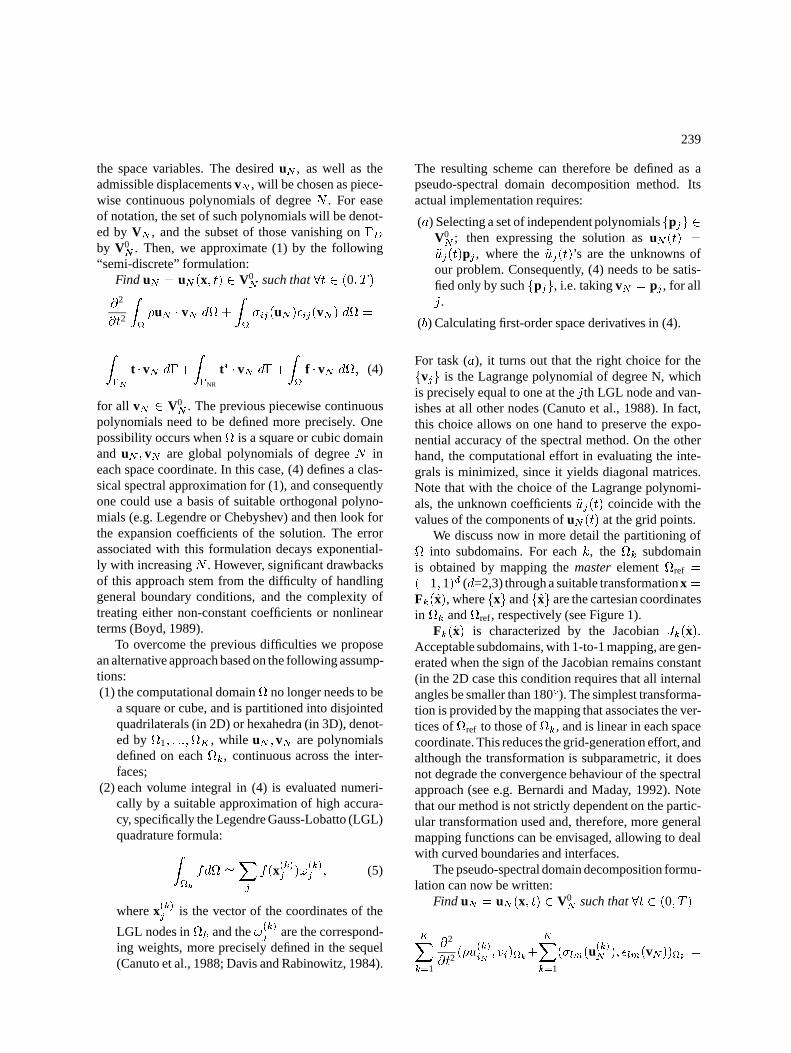
The resulting scheme can therefore be defined as apseudo-spectral domain decomposition method. Itsactual implementation requires:

(a) Selecting a set of independent polynomialsfpjg 2V0N ; then expressing the solution asuN (t) =

~uj(t)pj , where the~uj(t)’s are the unknowns ofour problem. Consequently, (4) needs to be satis-fied only by suchfpjg, i.e. takingvN = pj , for allj.

(b) Calculating first-order space derivatives in (4).

For task (a), it turns out that the right choice for thefvjg is the Lagrange polynomial of degree N, whichis precisely equal to one at thejth LGL node and van-ishes at all other nodes (Canuto et al., 1988). In fact,this choice allows on one hand to preserve the expo-nential accuracy of the spectral method. On the otherhand, the computational effort in evaluating the inte-grals is minimized, since it yields diagonal matrices.Note that with the choice of the Lagrange polynomi-als, the unknown coefficients~uj(t) coincide with thevalues of the components ofuN (t) at the grid points.

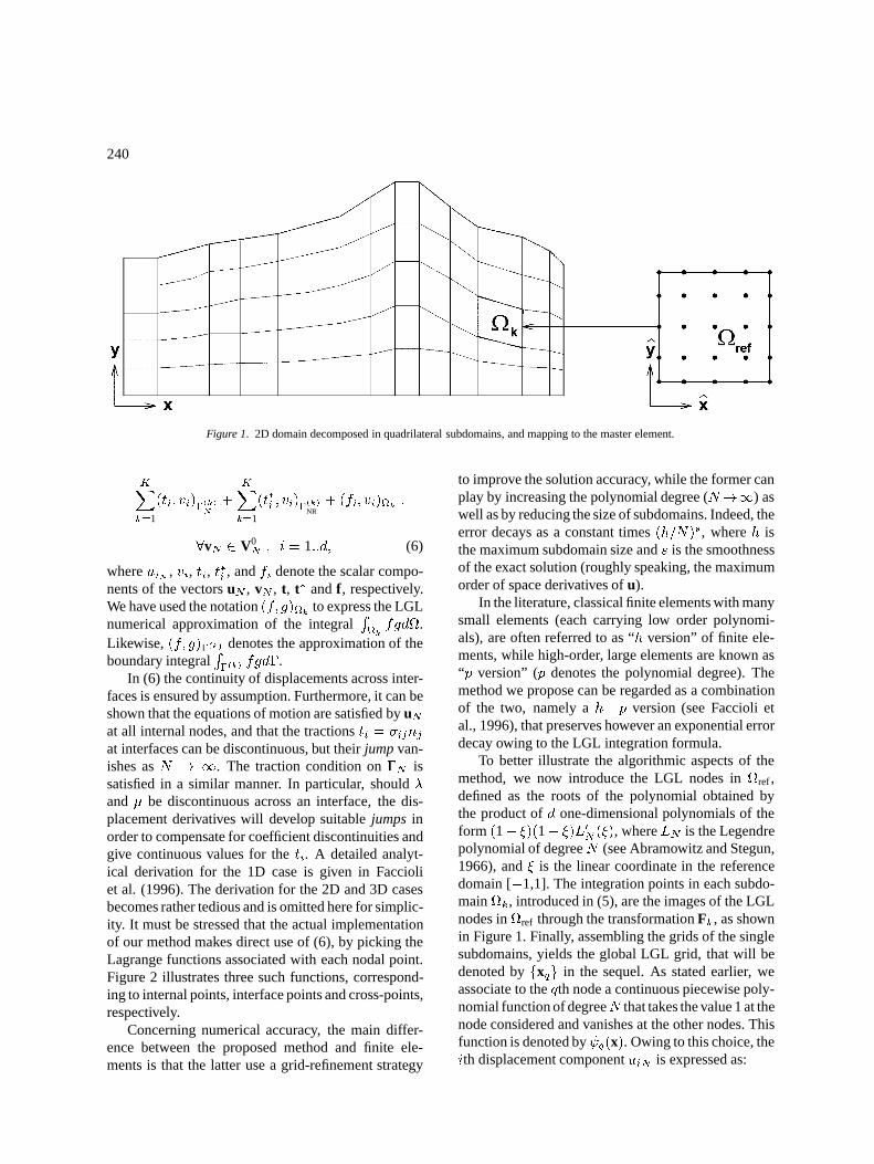
We discuss now in more detail the partitioning of into subdomains. For eachk, the k subdomainis obtained by mapping themasterelementref =(�1; 1)d (d=2,3) through a suitable transformationx =Fk(x), wherefxg andfxg are the cartesian coordinatesin k andref, respectively (see Figure 1).

Fk(x) is characterized by the JacobianJk(x).Acceptable subdomains, with 1-to-1 mapping, are gen-erated when the sign of the Jacobian remains constant(in the 2D case this condition requires that all internalangles be smaller than 180�). The simplest transforma-tion is provided by the mapping that associates the ver-tices ofref to those ofk, and is linear in each spacecoordinate. This reduces the grid-generation effort,andalthough the transformation is subparametric, it doesnot degrade the convergence behaviour of the spectralapproach (see e.g. Bernardi and Maday, 1992). Notethat our method is not strictly dependent on the partic-ular transformation used and, therefore, more generalmapping functions can be envisaged, allowing to dealwith curved boundaries and interfaces.

The pseudo-spectral domain decomposition formu-lation can now be written:

Find uN = uN (x; t) 2 V0N such that8t 2 (0; T )

KXk=1

@2

@t2(�u

(k)iN; vi)k+

KXk=1

(�lm(u(k)N ); �lm(vN))k =

jose17.tex; 21/01/1998; 23:12; v.7; p.3

240

Figure 1. 2D domain decomposed in quadrilateral subdomains, and mapping to the master element.

KXk=1

(ti; vi)�(k)

N

+

KXk=1

(t�i ; vi)�(k)NR

+ (fi; vi)k ;

8vN 2 V0N ; i = 1::d; (6)

whereuiN , vi, ti, t�i , andfi denote the scalar compo-nents of the vectorsuN , vN , t, t� andf , respectively.We have used the notation(f; g)k to express the LGLnumerical approximation of the integral

Rkfgd.

Likewise,(f; g)�(k) denotes the approximation of theboundary integral

R�(k) fgd�.

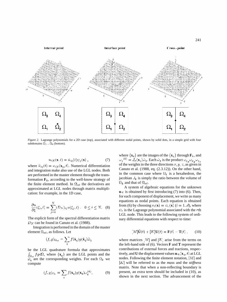
In (6) the continuity of displacements across inter-faces is ensured by assumption. Furthermore, it can beshown that the equations of motion are satisfied byuNat all internal nodes, and that the tractionsti = �ijnjat interfaces can be discontinuous, but theirjumpvan-ishes asN ! 1. The traction condition on�N issatisfied in a similar manner. In particular, should�and� be discontinuous across an interface, the dis-placement derivatives will develop suitablejumps inorder to compensate for coefficient discontinuities andgive continuous values for theti. A detailed analyt-ical derivation for the 1D case is given in Faccioliet al. (1996). The derivation for the 2D and 3D casesbecomes rather tedious and is omitted here for simplic-ity. It must be stressed that the actual implementationof our method makes direct use of (6), by picking theLagrange functions associated with each nodal point.Figure 2 illustrates three such functions, correspond-ing to internal points, interface points and cross-points,respectively.

Concerning numerical accuracy, the main differ-ence between the proposed method and finite ele-ments is that the latter use a grid-refinement strategy

to improve the solution accuracy, while the former canplay by increasing the polynomial degree (N!1) aswell as by reducing the size of subdomains. Indeed, theerror decays as a constant times(h=N)s, whereh isthe maximum subdomain size ands is the smoothnessof the exact solution (roughly speaking, the maximumorder of space derivatives ofu).

In the literature, classical finite elements with manysmall elements (each carrying low order polynomi-als), are often referred to as “h version” of finite ele-ments, while high-order, large elements are known as“p version” (p denotes the polynomial degree). Themethod we propose can be regarded as a combinationof the two, namely ah�p version (see Faccioli etal., 1996), that preserves however an exponential errordecay owing to the LGL integration formula.

To better illustrate the algorithmic aspects of themethod, we now introduce the LGL nodes inref,defined as the roots of the polynomial obtained bythe product ofd one-dimensional polynomials of theform (1� �)(1+ �)L0N (�), whereLN is the Legendrepolynomial of degreeN (see Abramowitz and Stegun,1966), and� is the linear coordinate in the referencedomain [�1,1]. The integration points in each subdo-maink, introduced in (5), are the images of the LGLnodes inref through the transformationFk, as shownin Figure 1. Finally, assembling the grids of the singlesubdomains, yields the global LGL grid, that will bedenoted byfxqg in the sequel. As stated earlier, weassociate to theqth node a continuous piecewise poly-nomial function of degreeN that takes the value 1 at thenode considered and vanishes at the other nodes. Thisfunction is denoted by q(x). Owing to this choice, theith displacement componentuiN is expressed as:

jose17.tex; 21/01/1998; 23:12; v.7; p.4

241

Figure 2. Lagrange polynomials for a 2D case (top), associated with different nodal points, shown by solid dots, in a simple grid with foursubdomains1 ..4 (bottom).

uiN (x; t) = ~uiq(t) q(x) ; (7)

where~uiq(t) = uiN (xq; t). Numerical differentiationand integration make also use of the LGL nodes. Bothare performed in the master element through the trans-formationFk, according to the well-know strategy ofthe finite element method. Inref the derivatives areapproximated at LGL nodes through matrix multipli-cation: for example, in the 1D case,

@u

@�(�i; t) =

NXj=0

(DN )iju(�j ; t) ; 0� i � N: (8)

The explicit form of the spectral differentiation matrixDN can be found in Canuto et al. (1988).

Integration is performed in the domain of the masterelementref, as follows. Let

(f; g)ref =Xq

f(xq)g(xq)!q

be the LGL quadrature formula that approximatesRref

fgd, wherefxqg are the LGL points and the!q are the corresponding weights. For eachk wecompute

(f; g)k =Xq

f(xq)g(xq)!(k)q ; (9)

wherefxqg are the images of thefxqg throughFk, and!q

(k) = Jk(xq)!q . Each!q is the product!qx!qy!qzof the weights in the three directionsx; y; z, as given inCanuto et al. (1988, eq. (2.3.12)). On the other hand,in the common case wherek is a hexahedron, thejacobianJk is simply the ratio between the volume ofk and that ofref.

A system of algebraic equations for the unknownuN is obtained by first introducing (7) into (6). Then,for each component of displacement, we write as manyequations as nodal points. Each equation is obtainedfrom (6) by choosingvi(x) = r(x) (i = 1::d), where r is the Lagrange polynomial associated with therthLGL node. This leads to the following system of ordi-nary differential equations with respect to time:

[M ]�U(t) + [K]U(t) = F(t) + T(t) ; (10)

where matrices[M ] and [K] arise from the terms onthe left-hand side of (6). VectorsF andT represent thecontributions of external forces and tractions, respec-tively, andU the displacement valuesuN (xq ; t) at LGLnodes. Following the finite element notation,[M ] and[K] will be referred to as themassand thestiffnessmatrix. Note that when a non-reflecting boundary ispresent, an extra term should be included in (10), asshown in the next section. The advancement of the

jose17.tex; 21/01/1998; 23:12; v.7; p.5

242

numerical solution of (10) in time will be discussed ina later section.

Non-reflecting boundaries

It was mentioned in the previous section that a custom-ary approach for dealing with infinite media consistsof introducing a fictitious boundary and setting absorb-ing conditions on it. These can be naturally formulatedin the frequency domain, while they lead to non-localconditions (both in space and time) when included inspace-time methods like the present one. For this rea-son, a number of local non-reflecting conditions havebeen proposed, based on the paraxial approximation ofthe wave equation (Clayton and Engquist, 1977) andcharacterized by the following features:

(i) they are exact for normal wave incidence (�=0�),but their efficiency degrades for increasing� and isminimal for parallel incidence (�=90�);

(ii) a family of paraxial approximations with increas-ing efficiency exists, based on homogeneous linearcombinations of space-time derivatives of the solu-tion.

A straightforward variational treatment is possiblewhen the non-reflecting condition can be directly sub-stituted in the traction term contained in the integral on�NR of (1). For this reason we presently limit ourselvesto first order conditions. Among these, the so-called P3paraxial conditions due to Stacey (1988) were provedto be effective and stable over a rather wide range ofthe elastic parameters, and are adopted in this paper.Stability is ensured for Poisson coefficient� � 0.33,approximately.

Substituting the P3 conditions of Stacey into theintegral on�NR of (1), and performing the spectralapproximation procedure, leads to the system

[M ]�U(t) + [A] _U(t) + [K]U(t) = F(t) + T(t) : (11)

The matrix [A] arises from time derivatives in con-ditions P3, and is clearly equivalent to introducing a(radiation) damping term into the problem.

Time discretization

The full numerical treatment of the problem requiresthe time-discretization of (11). Due to the presence ofthe first order paraxial conditions on the�NR part ofthe boundary, an appropriate time-marching schemeshould handle simultaneously the first and second timederivatives without compromising the overall accura-cy and stability. Several finite difference schemes havebeen tested for the scalar 2D wave equation (Mag-gio and Quarteroni, 1994), both implicit and explicit.While the former are unconditionally stable, the lattermust satisfy the Courant-Friedrichs-Levy (CFL) con-dition

�t � ��xmin

cmax; (12)

where�xmin is the minimum spectral grid spacing,cmax is an upper bound for the wave propagation veloc-ity, and � is a positive constant strictly less than 1.Since�xmin corresponds to the LGL points closest tothe boundary, where the spectral grid size is propor-tional toN�2, the condition for numerical stability canalso be written as:

�t �L

N2

��

cmax; (13)

whereL is the typical linear dimension ofk. Inthe particular caseN=5, used in present applications,�� '4.3�.

Condition (13) shows that the stability requirementon�t becomes prohibitive for small values ofL=N2

(which correspond to thep-version), for which animplicit time discretization is strongly recommended.For theh andh-p version, the best tradeoff in termsof accuracy, stability and computational complexity(also in view of parallel computing), is provided by theexplicit 2nd order (leap-frog) scheme LF2-LF2, basedon the following approximations:

( �@2u@t2

�n= 1

(�t)2 (un+1 � 2un + un�1) +O((�t)2)�@u@t

�n= 1

2�t (un+1 � un�1) +O((�t)2)

jose17.tex; 21/01/1998; 23:12; v.7; p.6

243

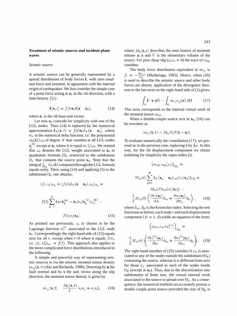
Treatment of seismic sources and incident planewaves

Seismic source

A seismic source can be generally represented by aspatial distribution of body forcesf , with zero resul-tant force and moment, in agreement with the internalorigin of earthquakes. We first consider the simple caseof a point force acting atx0 in theith direction, with atime-historyf(t):

f (x; t) = f(t)ei�(x� x0); (14)

whereei is theith base unit vector.Let nowx0 coincide for simplicity with one of the

LGL nodes. Then (14) is replaced by the numericalapproximationfN (x; t) = f(t)ei�N (x � x0), where�N is the numerical delta function, i.e. the polynomial 0(x)=!0 of degreeN that vanishes at all LGL nodesx(k)j except atx0 where it is equal to 1=!0. We remindthat !0 denotes the LGL weight associated tox0 inquadrature formula (5), restricted to the subdomaink that contains the source pointx0. Note that theintegral

Rk�Nd computed through the LGL formula

equals unity. Then, using (14) and applying (5) to thesubdomaink one obtains:

(fi; vi)k = (f(t)�N (x� x0); vi)k =

f(t)

NXq=1

�N (x(k)q � x0)vi(x(k)q )!(k)

j =

f(t)vi(x0): (15)

As pointed out previously,vi is chosen to be theLagrange function (i)r associated to the LGL nodexr. Correspondingly the right-hand side of (15) equalszero for allr, except whenr=0 where it equalsf(t),i.e. (fi; i0)k = f(t). This approach also applies tothe more complicated force distributions introduced inthe following.

A simple and powerful way of representing seis-mic sources is via the seismic moment tensor densitymij(x; t) (Aki and Richards, 1980). Denoting byn thefault normal and bys the unit vector along the slipdirection, the moment tensor density is given by

mij(x; t) =M0(x; t)

V[sinj + sjni]; (16)

whereM0(x; t) describes the time history of momentrelease atx andV is the elementary volume of thesource. For pure shear slip (sini = 0) the trace ofmij

vanishes.The body force distribution equivalent tomij is

fi = �@mij

@xj(Madariaga, 1983). Hence, when (16)

is used to describe the seismic source and other bodyforces are absent, application of the divergence theo-rem to the last term on the right-hand side of (1) gives:Z

f � v d =

Z

mij�ij(v) d: (17)

This term corresponds to the internal virtual work ofthe moment tensormij .

When a double-couple source acts inx0, (16) canbe rewritten as

mij(x; t) =Mij(t)�(x� x0):

To evaluate numerically the contribution (17), we pro-ceed as in the previous case, replacing� by �N . In thisway, for theith displacement component we obtain(omitting for simplicity the super-indexk):

�mnl; �nl(vi)

�k

=

Mnl(t)

NXq=1

�N (xq � x0)�nl(vi(xq))!q =

Mnl(t)�nl(vi(x0)) =

12Mnl(t)

�@vi(x0)

@xl�ni +

@vi(x0)

@xn�li

�; (18)

where�ni, �li is the Kronecker index. Selecting the testfunctions as before, each noder and each displacementcomponenti (i = 1::d) yields an equation of the form:�

mnl; �nl( (i)r )�k

=

12Mnl(t)

@

(i)r (x0)

@xl�ni +

@ (i)r (x0)

@xn�li

!: (19)

The right-hand member of (19) vanishes if r is asso-ciated to any of the nodes outside the subdomain (k)containing the source, whereas it is different from zerofor those r associated to each of the nodes insidek (except atx0). Thus, due to the discretization intosubdomains of finite size, the virtual internal workassociated to the source is spread overk. As a conse-quence, the numerical method can accurately portray adouble couple point source provided the size ofk is

jose17.tex; 21/01/1998; 23:12; v.7; p.7

244

small compared to the significant wavelengths of theanalysis.

Plane wave

A vertically incident plane wave of displacement alongthe i-direction, having an assigned time-dependence�ui(t), can be efficiently introduced through an appro-priate distribution of body forcesf (x; t). These areapplied at the nodes of a horizontal grid line near thebottom boundary of the computational domain and aredetermined as follows.

In a 3D infinite homogeneous medium, the dis-placement in thei-direction generated by a uniformdistribution of body forcesf (z; t) = �(t)�(z � z0)eiacting on the planez = z0, is given by

ui(z; t) =1

2�cH(t�

jz � z0j

c)

Z t�jz�z0j

c

0�(�)d�;

(20)wherec is the propagation velocity andH(�) the stepfunction. Hence, in order to propagate an assigneddisplacement waveform�ui(t), we determine the timedependence of the force distribution by differentiating(20) with respect to time and evaluating the result atz = z0. This yields

�(t) = 2�c@�ui(t)

@t: (21)

The analytical derivation of (20), see e.g. Graff (1975),involves the integral

R1

�1�(z � z0)dz. Our numerical

approximation should result in a unit value of suchintegral. Since integration is now performed in thez-direction only, we take the numerical delta functionto be the Lagrange polynomial of degreeN that van-ishes at all LGL nodes except atz = z0, where itequals 1

!0z, according to the definitions given after (9).

Subsequently, the introduction of the force distributionf (z; t) in the numerical scheme leads to the approxi-mation (15) at all LGL nodes.

Applications

Validations with 2D theoretical solutions

We illustrate first the performance of the proposedmethod, in the so-calledh� p version (relatively lowN and many small subdomains), for two classical 2D

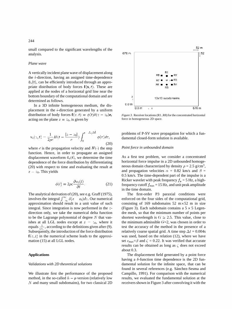
Figure 3. Receiver locations (R1..R8) for the concentrated horizontalforce in homogeneous 2D space.

problems of P-SV wave propagation for which a fun-damental closed-form solution is available.

Point force in unbounded domain

As a first test problem, we consider a concentratedhorizontal force impulse in a 2D unbounded homoge-neous domain characterized by density� = 2.5 g/cm3,and propagation velocities� = 0.82 km/s and� =0.5 km/s. The time-dependent part of the impulse is aRicker wavelet with peak frequencyfp = 5 Hz, a high-frequency cutofffmax= 15 Hz, and unit peak amplitudein the time domain.

The first-order P3 paraxial conditions wereenforced on the four sides of the computational grid,consisting of 169 subdomains 52 m�52 m in size(Figure 3). Each subdomain contains a 5�5 Legen-dre mesh, so that the minimum number of points pershortest wavelength isG ' 2.5. This value, close tothe minimum admissibleG=2, was chosen in order totest the accuracy of the method in the presence of arelatively coarse spatial grid. A time step�t = 0.004swas used, based on the relation (12), where we havesetcmax=� and� = 0.22. It was verified that accurateresults can be obtained as long as� does not exceedabout 0.3.

The displacement field generated by a point forcehaving a�-function time dependence is the 2D fun-damental solution for the infinite space, that can befound in several references (e.g. Sanchez-Sesma andCampillo, 1991). For comparison with the numericalresults, we evaluated the fundamental solution at thereceivers shown in Figure 3 after convolving it with the

jose17.tex; 21/01/1998; 23:12; v.7; p.8

245

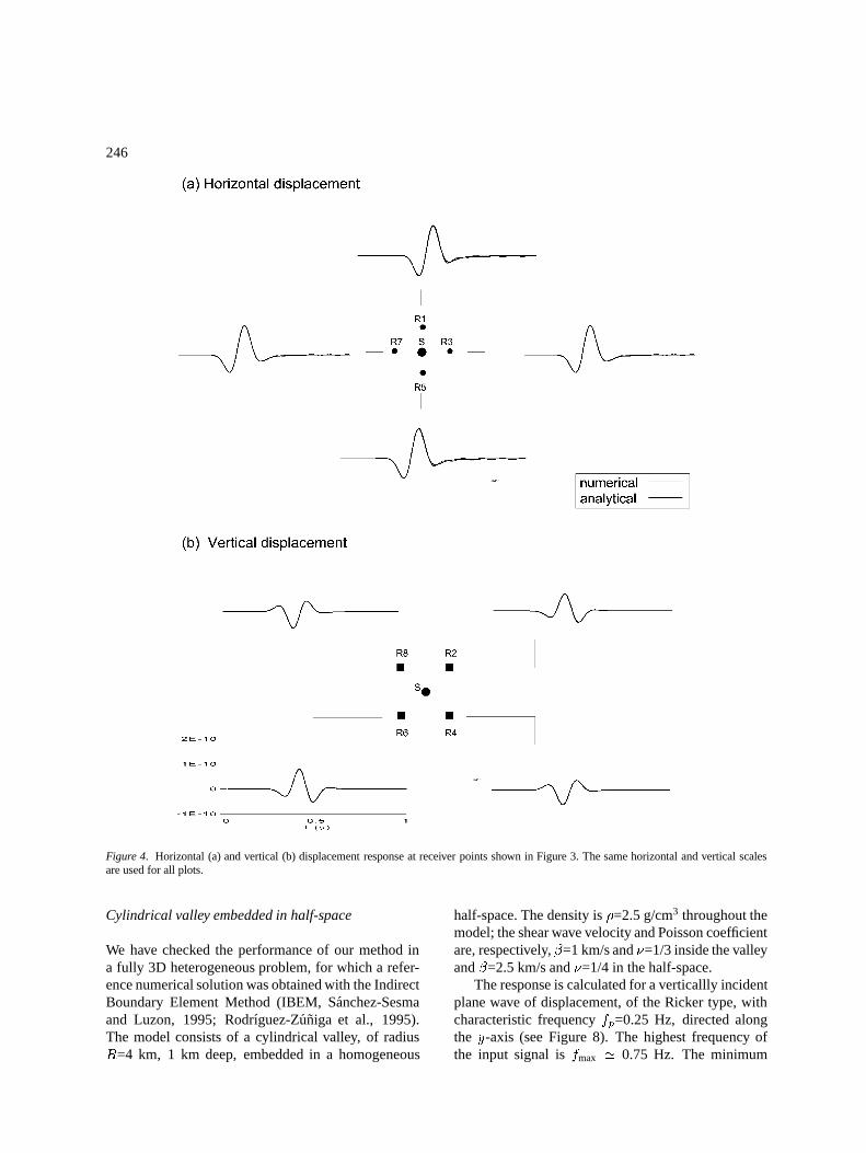
Ricker wavelet that describes the time dependence ofthe applied force. The horizontal and vertical displace-ments are displayed in Figure 4(a) and (b) at differentreceivers, to highlight the properties of symmetry andanti-symmetry of the solution. The numerical verticaldisplacements appear almost undistinguishable fromthe theoretical ones, while the horizontal displace-ments are affected by very small oscillations followingthe main pulse. These are dispersion errors arising fromthe lowG value, and we checked that they disappearwhen a finer spatial grid (G=4) is used.

Pressure source buried in half-space (Garvin’sproblem)

As a further case of 2D in-plane wave propagationwe take the generation of transient disturbances froma line source of pressure buried under the surface ofa homogeneous half-space. An elegant closed-formsolution to this problem, based on Laplace Transformtechniques, has been found by Garvin (1956) for a step-function time-dependence of the source. This solutionshows well the progressive build-up of a prominentRayleigh pulse with incresing epicentral distance.

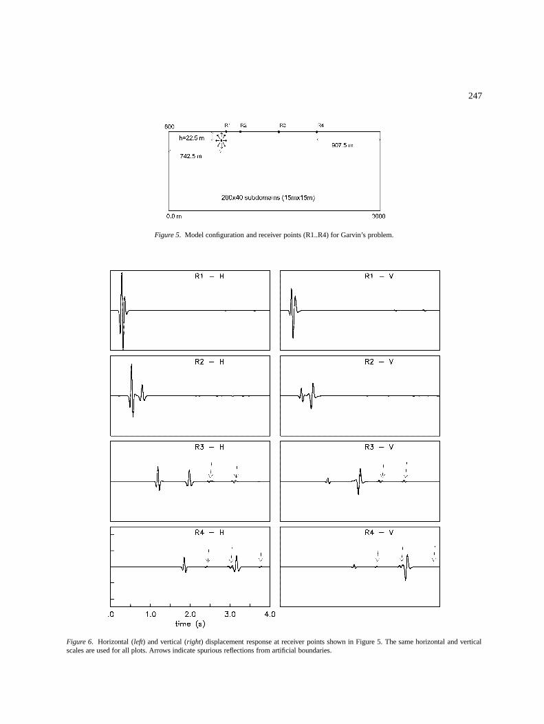
We analysed the configuration illustrated in Figure5, using the same material properties as in the previousexample. The source depth ish = 22.5 m and severalreceivers are placed on the surface at a spacingd=h= 3 or 6, and maximum distance 60d=h. The sourcedepth is shallow so as to maximize the emergence ofthe Rayleigh wave and, hence, to allow a completetest of the free boundary condition of our method. Thepressure source is introduced as the gradient of a scalarpotential that has the form of a gaussian function inspace, centered at the location of the source with non-zero values over a small region of the grid having thesame dimensions as a single subdomain (Kosloff et al.,1984). The time dependence of the source is describedby a Ricker wavelet with unit peak amplitude in time,fp = 10 Hz, andfmax = 30 Hz , which gives a shortestinput wavelength of 16.6 m.

To minimise residual reflections from the bound-aries, a relatively large rectangular computationaldomain is adopted, and this is partitioned into 800square subdomains of 15 m�15 m and 5�5 Legen-dre mesh, resulting inG ' 4. This choice of gridspacing is dictated less by the requirement of avoidingdispersion, than by the need to keep the source con-fined within a small region and approach the conditionof a point source. A time step of 0.001 sec has beenused. The analytical displacements for the chosen time-

dependence of the source were derived from Garvin’sclosed-form solution using an especially developedcomputational procedure (Sanchez-Sesma, 1996). Thenumerical displacements are portrayed in Figure 6 andexhibit the expected strong Rayleigh pulse, especial-ly prominent in the vertical component. Because ofthe low geometric attenuation, at the larger distancesthe pulse travels almost unchanged at the theoreticallypredicted phase velocity of about 450 m/s. The numer-ical seismograms agree very closely with the analyticalones, although in their late parts they are affected bylow-amplitude spurious pulses (especially at receiversR3 and R4) generated mainly by the bottom absorbingboundary.

Validations with 3D solutions

Double-couple solution in an infinite space

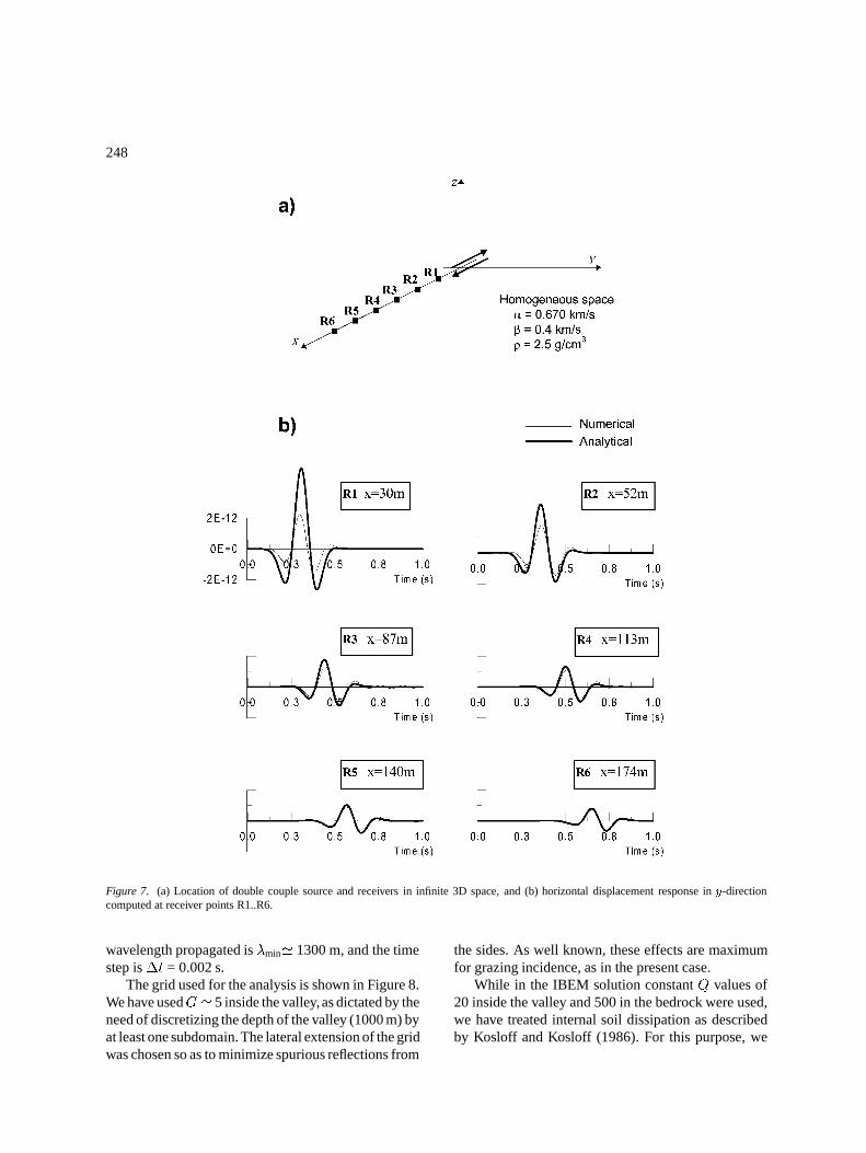
As a first 3D test, the performance of the pseudo-spectral method is checked against the fundamen-tal solution (see e.g. Aki and Richards, 1980) for apoint double couple source in an homogeneous infi-nite space. In the analytical solution, all contributions(near-field, intermediate and far-field) were consid-ered. The geometry of the problem is summarized inFigure 7(a): the double couple acts at the origin ofthe coordinate system, with the fault contained in thex� z plane and slip directed along thex-axis. Densityis �=2.5 g/cm3; the propagation velocity of P and Swaves is�=0.67 km/s and�=0.4 km/s, respectively.The input signal is a Ricker wavelet with fundamen-tal frequencyfp=4 Hz and high-frequency cutoff atfmax=12 Hz. The computational subdomains are cubeswith 52 m side, each containing 5�5�5 grid points.The shortest wavelength propagated is�=33 m, so thatG '2.5 has been used in this analysis. The time stepis�t=0.005 s, corresponding to�=0.22 in (12).

The displacements in they-direction are comparedin Figure 7(b) for a row of six receivers along thex-axis; the exact position of the receivers is indicatedin the same figure. The analytical and numerical solu-tions tend to coincide for a source distancer� 100 m,which is approximately the fundamental wavelength ofS-waves. As previously pointed out, the lack of agree-ment close to the source can be attributed to the numer-ical spreading of the double couple over the whole sub-domain where it is applied, so that it can no longer beconsidered as a true point source. Hence, to accurate-ly portray the near-field motion, smaller subdomainsshould be used for the source region.

jose17.tex; 21/01/1998; 23:12; v.7; p.9

246

Figure 4. Horizontal (a) and vertical (b) displacement response at receiver points shown in Figure 3. The same horizontal and vertical scalesare used for all plots.

Cylindrical valley embedded in half-space

We have checked the performance of our method ina fully 3D heterogeneous problem, for which a refer-ence numerical solution was obtained with the IndirectBoundary Element Method (IBEM, Sanchez-Sesmaand Luzon, 1995; Rodrıguez-Zuniga et al., 1995).The model consists of a cylindrical valley, of radiusR=4 km, 1 km deep, embedded in a homogeneous

half-space. The density is�=2.5 g/cm3 throughout themodel; the shear wave velocity and Poisson coefficientare, respectively,�=1 km/s and�=1/3 inside the valleyand�=2.5 km/s and�=1/4 in the half-space.

The response is calculated for a verticallly incidentplane wave of displacement, of the Ricker type, withcharacteristic frequencyfp=0.25 Hz, directed alongthe y-axis (see Figure 8). The highest frequency ofthe input signal isfmax ' 0.75 Hz. The minimum

jose17.tex; 21/01/1998; 23:12; v.7; p.10

247

Figure 5. Model configuration and receiver points (R1..R4) for Garvin’s problem.

Figure 6. Horizontal (left) and vertical (right) displacement response at receiver points shown in Figure 5. The same horizontal and verticalscales are used for all plots. Arrows indicate spurious reflections from artificial boundaries.

jose17.tex; 21/01/1998; 23:12; v.7; p.11

248

Figure 7. (a) Location of double couple source and receivers in infinite 3D space, and (b) horizontal displacement response iny-directioncomputed at receiver points R1..R6.

wavelength propagated is�min' 1300 m, and the timestep is�t = 0.002 s.

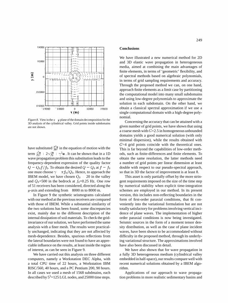
The grid used for the analysis is shown in Figure 8.We have usedG ' 5 inside the valley,as dictated by theneed of discretizing the depth of the valley (1000 m) byat least one subdomain.The lateral extension of the gridwas chosen so as to minimize spurious reflections from

the sides. As well known, these effects are maximumfor grazing incidence, as in the present case.

While in the IBEM solution constantQ values of20 inside the valley and 500 in the bedrock were used,we have treated internal soil dissipation as describedby Kosloff and Kosloff (1986). For this purpose, we

jose17.tex; 21/01/1998; 23:12; v.7; p.12

249

Figure 8. View in thex�y plane of the domain decomposition for the3D analysis of the cylindrical valley. Grid points inside subdomainsare not shown.

have substituted@2u@t2 in the equation of motion with the

term @2u@t2 + 2 @u

@t+ 2u . It can be shown that in a 1D

wave propagationproblem this substitution leads to thefrequency-dependent expression of the quality factorQ = Q0f=f0. To obtain the desiredQ = Q0 atf = f0

one must choose = �f0=Q0. Hence, to approach theIBEM model, we have chosenQ0 = 20 in the valleyandQ0=500 in the bedrock atf0=0.25 Hz. One rowof 51 receivers has been considered, directed along they-axis and extending from�8000 m to 8000 m.

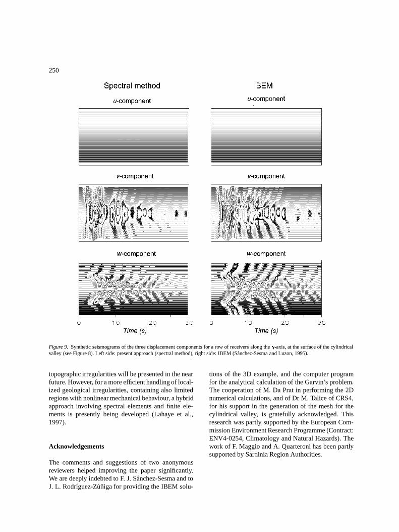
In Figure 9 the synthetic seismograms calculatedwith our method at the previous receivers are comparedwith those of IBEM. While a substantial similarity ofthe two solutions has been found, some discrepanciesexist, mainly due to the different description of theinternal dissipation of soil materials. To check the grid-invarianceof our solution, we have performed the sameanalysis with a finer mesh. The results were practical-ly unchanged, indicating that they are not affected bymesh-dependence. Besides, spurious reflections fromthe lateral boundaries were not found to have an appre-ciable influence on the results, at least inside the regionof interest, as can be seen in Figure 9.

We have carried out this analysis on three differentcomputers, namely a Workstation DEC Alpha, witha total CPU time of 22 hours, a Workstation IBMRISC/560, 40 hours, and a PC Pentium 200, 90 hours.In all cases we used a mesh of 1568 subdmains, eachdescribed by 53=125 LGL nodes, and 25000 time steps.

Conclusions

We have illustrated a new numerical method for 2Dand 3D elastic wave propagation in heterogeneousmedia, aimed at combining the main advantages offinite elements, in terms of ‘geometric’ flexibility, andof spectral methods based on algebraic polynomials,in terms of grid sampling requirements and accuracy.Through the proposed method we can, on one hand,approach finite elements as a limit case by partitioningthe computational model into many small subdomainsand using low-degree polynomials to approximate thesolution in each subdomain. On the other hand, weobtain a classical spectral approximation if we use asingle computational domain with a high-degree poly-nomial.

Concerning the accuracy that can be attained with agiven number of grid points, we have shown that usinga coarse mesh withG=2.5 in homogeneous unboundeddomains yields a good numerical solution (with onlyminimal dispersion), while the results obtained withG=4 grid points coincide with the theoretical ones.This is far beyond the capabilities of low-order meth-ods, such as finite-differences and finite elements. Toobtain the same resolution, the latter methods needa number of grid points per linear dimension at leastdouble with respect to our pseudo-spectral approach,so that in 3D the factor of improvement is at least 8.

This asset is only partially offset by the more strin-gent requirements imposed on the size of the time stepby numerical stability when explicit time-integrationschemes are employed in our method. In its presentversion, this includes non-reflecting boundaries in theform of first-order paraxial conditions, that fit con-veniently into the variational formulation but are nottotally satisfactory for problems involving vertical inci-dence of plane waves. The implementation of higherorder paraxial conditions is now being investigated.Seismic sources in the form of a moment tensor den-sity distribution, as well as the case of plane incidentwaves, have been shown to be accommodated withoutdifficulty in the proposed method, through its underly-ing variational structure. The approximations involvedhave also been discussed in detail.

We have also shown that for wave propagation ina fully 3D heterogeneous medium (cylindrical valleyembedded in half-space),our results compare well withrecent numerical solutions obtained by a IBEM algo-rithm.

Applications of our approach to wave propaga-tion problems in more realistic sedimentary basins and

jose17.tex; 21/01/1998; 23:12; v.7; p.13

250

Figure 9. Synthetic seismograms of the three displacement components for a row of receivers along they-axis, at the surface of the cylindricalvalley (see Figure 8). Left side: present approach (spectral method), right side: IBEM (Sanchez-Sesma and Luzon, 1995).

topographic irregularities will be presented in the nearfuture. However, for a more efficient handling of local-ized geological irregularities, containing also limitedregions with nonlinear mechanical behaviour, a hybridapproach involving spectral elements and finite ele-ments is presently being developed (Lahaye et al.,1997).

Acknowledgements

The comments and suggestions of two anonymousreviewers helped improving the paper significantly.We are deeply indebted to F. J. Sanchez-Sesma and toJ. L. Rodrıguez-Zuniga for providing the IBEM solu-

tions of the 3D example, and the computer programfor the analytical calculation of the Garvin’s problem.The cooperation of M. Da Prat in performing the 2Dnumerical calculations, and of Dr M. Talice of CRS4,for his support in the generation of the mesh for thecylindrical valley, is gratefully acknowledged. Thisresearch was partly supported by the European Com-mission Environment Research Programme (Contract:ENV4-0254, Climatology and Natural Hazards). Thework of F. Maggio and A. Quarteroni has been partlysupported by Sardinia Region Authorities.

jose17.tex; 21/01/1998; 23:12; v.7; p.14

251

References

Abramowitz, M. and Stegun, I. A. (eds), 1966,Handbook of Math-ematical Functions, Dover, New York.

Aki K. and Richards, P., 1980,Quantitative Seismology. Theory andMethods, Freeman, San Francisco.

Bernardi, C. and Maday, Y., 1992,Approximations Spectrales deProblemes aux Limites Elliptiques, Springer-Verlag, Paris.

Boyd, J. P., 1989,Chebyshev and Fourier Spectral Methods,Springer-Verlag, Berlin.

Canuto, C., Hussaini, M., Quarteroni, A. and Zang, T., 1988,Spec-tral Methods in Fluid Dynamics, Springer-Verlag, New York.

Clayton, R. and Engquist, B., 1977, Absorbing boundary conditionsfor acoustic and elastic wave equations,B.S.S.A.67, 1529–1540.

Davis, P. and Rabinowitz, P., 1984,Methods of Numerical Integra-tion, 2nd edn., Academic Press, Orlando.

Faccioli, E., Maggio, F., Quarteroni, A. and Tagliani, A., 1996,Spectral-domain decomposition methods for the solution ofacoustic and elastic wave equations,Geophysics61, 1160-1174.

Frankel, A. and Vidale, J., 1992, A three-dimensional simulation ofseismic waves in the Santa Clara Valley, California, from a LomaPrieta aftershock,B.S.S.A.82, 2045–2074.

Frankel, A., 1993, Three-dimensional simulations of ground motionsin the San Bernardino Valley, California, for hypothetical earth-quakes on the San Andreas fault,B.S.S.A.83, 1020–1041.

Garvin, W., 1956, Exact transient solution of the buried line sourceproblem,Proc. Royal Soc. London, Series A234, 528–541.

Graff, K. F., 1975,Wave Motion in Elastic Solids, Oxford UniversityPress, London.

Graves, R., 1996, Simulating seismic wave propagation in 3D elasticmedia using staggered-grid finite differences,B.S.S.A.86, 1091–1106.

Kosloff, D., Reshef, M. and Loewenthal, D., 1984, Elastic wavecalculations by the Fourier method.B.S.S.A.74, 875–891.

Kosloff, R. and Kosloff, D., 1986, Absorbing boundaries for wavepropagation problems,J. Comp. Phys.63, 363–376.

Lahaye, D., Maggio, F. and Quarteroni, A., 1997, Hybrid spectralelement - finite element methods for wave propagation problems.To appear inEast–West J. Num. Math..

Madariaga, R., 1983, Earthquake source theory: a review. In:Proc.Int. School of Physics "E. Fermi", Course 85, Varenna, Italy,1–44, North-Holland, Amsterdam.

Maggio, F. and Quarteroni, A., 1994, Acoustic wave simulation byspectral methods.East–West J. Num. Math.2, 129–150.

Olsen, K., Pechmann, J. and Schuster, G., 1995a, Simulation of3D elastic wave propagation in the Salt Lake Basin,B.S.S.A.85,1688–1710.

Olsen, K., Archuleta, R. and Matarese, J., 1995b, Three-dimensionalsimulation of a magnitude 7.75 earthquake on the San Andreasfault, Science270, 1628–1632.

Olsen, K., Pechmann, J. and Schuster, G., 1996, An analysis of sim-ulated and observed blast records in the Salt Lake basin,B.S.S.A.86, 1061–1076.

Rodrıguez-Zuniga, J. L., Sanchez-Sesma, F. J. and Perez-Rocha,L. E., 1995, Seismic response of shallow alluvial valleys: the useof simplified models,B.S.S.A.85, 890–899.

Sanchez-Sesma, F. J. and Campillo, M., 1991, Diffraction of P, SV,and Rayleigh waves by topographic features: a boundary integralformulation,B.S.S.A.81, 2234–2253.

Sanchez-Sesma, F. J. and Luzon, F., 1995, Seismic response ofthree-dimensional alluvial valleys for incident P, S, and Rayleighwaves,B.S.S.A.85, 269–284.

Sanchez-Sesma, F. J., 1996, Written personal communication.Stacey, R., 1988, Improved transparent boundary formulations for

the elastic-wave equation,B.S.S.A.78, 2089–2097.Zienkiewicz, O. C. and Taylor, R. L., 1989,The Finite Element

Method, Vol. 1, McGraw-Hill, London.

jose17.tex; 21/01/1998; 23:12; v.7; p.15