Four-wing attractors from pseudo to real

Papers

International Journal of Bifurcation and Chaos, Vol. 16, No. 4 (2006) 859–885c© World Scientific Publishing Company

FOUR-WING ATTRACTORS:FROM PSEUDO TO REAL

GUOYUAN QIDepartment of Automation,

Tianjin University of Science and Technology,Tianjin 300222, P. R. China

qi [email protected]

GUANRONG CHENDepartment of Electronic Engineering,

City University of Hong Kong,Hong Kong SAR, P. R. China

[email protected]

SHAOWEN LIDepartment of Mathematics,

Southwest University of Finance and Economics,Chengdu 610074, P. R. China

[email protected]

YUHUI ZHANGDepartment of Automation,

Tianjin University of Science and Technology,Tianjin 300222, P. R. China

Received February 16, 2005; Revised May 23, 2005

Some basic dynamical behaviors and the compound structure of a new four-dimensionalautonomous chaotic system with cubic nonlinearities are investigated. A four-wing chaoticattractor is observed numerically. This attractor, however, is shown to be an numerical artifactby further theoretical analysis and analog circuit experiment. The observed four-wing attractoractually has two coexisting (upper and lower) attractors, which appear simultaneously and arelocated arbitrarily closely in the phase space. By introducing a simple linear state-feedback con-trol term, some symmetries of the system and similarities of the linearized characteristics canbe destroyed, thereby leading to the appearance of some diagonal and anti-diagonal periodicorbits, through which the upper and lower attractors can indeed be merged together to form atruly single four-wing chaotic attractor. This four-wing attractor is real; it is further confirmedanalytically, numerically, as well as electronically in the paper. Moreover, by introducing a sign-switching control function, the system orbit can be manipulated so as to switch between twoequilibria or among four equilibria, generating two one-side double-wing attractors, which canalso be merged to yield a real four-wing attractor.

Keywords : Chaos; four-dimensional chaotic system; double-wing attractor; four-wing attractor;bifurcation; Lyapunov exponent; switching parameter.

859

860 G. Qi et al.

1. Introduction

Recently, within the engineering community therehas been considerable interest in studying chaoticdynamical systems and exploiting their propertiesfor possible technological applications [Chen & Yu,2003], in which much attention has been focusedon effectively generating chaotic attractors withmore complicated topological structures. In thisendeavor, there are two major efforts: generaliz-ing Chua’s circuits with multiscroll attractors andgeneralizing the Lorenz system with multiwingattractors.

In the efforts of generalizing Chua’s circuit[Chua et al., 1986] to produce multiscroll attractors,several effective techniques have been developedand some simple circuits have been designed andimplemented, including some generalized Chua’scircuits and cellular neural networks [Chua &Roska, 1993; Suykens & Chua, 1997]. More pre-cisely, a piecewise-linear (PWL) characteristic func-tion method was proposed to generate multiscrollattractors [Chua et al., 1986; Chua & Roska, 1993;Suykens & Vandewalle, 1993]. The essence of thesemethods is to add breakpoints in the PWL func-tion to increase the number of equilibria in asuitable way [Suykens & Chua, 1997]. A sine-function approach was then suggested for creatingmultiscroll chaotic attractors [Tang et al., 2001],in which the key is to change the locations ofthe equilibria. Later, a stair function was used forgenerating 1D-, 2D- and 3D-grid scroll attractors,which are located around the equilibria on a line,a plane, or a space, respectively [Yalcin et al.,2001a; Yalcin et al., 2002b]. More recently, severaldifferent nonlinear functions including switching,hysteresis and saturated functions were utilized forcreating chaotic attractors with multimerged basinsof attraction, or with multiscroll attractors thathave different desirable properties [Lu et al., 2003a;Lu et al., 2004b; Lu et al., 2004c; Han et al., 2005].

Note that the aforementioned methods for gen-erating multiscroll attractors have some commoncharacteristics:

(i) The nonlinearities of these systems are usu-ally not smooth functions; they are eitherpiecewise-linear continuous functions [Chuaet al., 1986; Chua & Roska, 1993; Suykens& Vandewalle, 1993; Suykens & Chua, 1997;Tang et al., 2001; Lu et al., 2004b], or dis-continuous ones such as the stair function[Yalcin et al., 2001a; Yalcin et al., 2002b],

switching function, and hysteresis-series func-tion [Lu et al., 2003; Han et al., 2005; Elwakilet al., 2000].

(ii) The basic techniques are either by increasingthe number of equilibria via PWL functionswith more breakpoints, or by stair or hysteri-sis functions to realize equilibrium jumping.

(iii) The number of scrolls equals to that of theequilibria.

(iv) The basic shape of the attractors is cyclic,called scroll. Viewing the shape of themultiscroll chaotic attractors, including 1-D n-scroll, 2-D n×m-scroll, and 3-D n×m× l scrollattractors, one can find that each scroll is arotating cycle moving around an equilibriumpoint.

On the other hand, when working with the clas-sical Lorenz system [Sparrow, 1982], the producedattractors typically have two wings in a butterflyshape [Baghious & Jarry, 1993; Elwakil & Kennedy,2001; Elwakil et al., 2002], but the number of wingsis not equal to that of the equilibria.

Based upon the concept of the generalizedLorenz system [Vanecek & Celikovsky, 1996],recently some similar but topologically nonequiv-alent chaotic systems were coined, including inparticular the Chen system, the Lu system, the gen-eralized Lorenz system family, and the hyperbolic-type of generalized Lorenz canonical form [Chen &Ueta, 1999; Lu & Chen, 2002; Chen & Lu, 2003;Celikovsky & Chen, 2002]. Same as the Lorenz sys-tem, all these Lorenz-like systems are smooth withtwo quadratic terms, have three equilibria, and pro-duce a double-wing attractor, although they bareall topologically nonequivalent with many differentcharacteristics.

To electronic engineers working on chaotic cir-cuits, generating multiscroll chaotic attractors isno longer a very difficult task [Chua et al., 1986;Suykens & Vandewalle, 1993; Yalcin et al., 2002b;Ozoguz et al., 2002; Suykens & Chua, 1997; Tanget al., 2001; Lu et al., 2004b; Lu et al., 2004c].However, how to generate multiwing chaotic attrac-tors remains a technical challenge today. A three-dimensional autonomous system, in which eachequation has a quadratic term, was recently intro-duced [Liu & Chen, 2003]. It is interesting to seethat this system, with five equilibria, can producea four-wing attractor (called “four-scroll attractor”in [Liu & Chen, 2003]), which is symmetric withrespect to the z-axis, but finally it was proved by

Four-Wing Attractors: From Pseudo to Real 861

the same authors to be a numerical artifact: itis not a real four-wing chaotic attractor but con-sists of two coexisting and closely located double-wing attractors [Liu & Chen, 2004]. Nevertheless, atrue four-wing attractor was generated by a three-dimensional autonomous quadratic chaotic systemwith five equilibria, under a feedback control input[Lu et al., 2004a].

Very recently, we have found a new four-dimensional autonomous chaotic system, in whicheach equation contains a cubic term [Qi et al.,2005]. This system has very rich nonlinear dynam-ics, including chaos, period-doubling bifurcations,sinks, sources, etc.

In this paper, some basic dynamical behav-iors and the compound structure of the new four-dimensional chaotic system found in [Qi et al., 2005]are further investigated. The system has gracefulsymmetries with respect to the x1 −x2 and x3 −x4

coordinate planes, as well as the origin, respectively,and has nine real equilibria which are divided intothree different types according to their linearizedcharacteristics. Of most interest is that a four-wing chaotic attractor can be observed numerically.However, careful theoretical analysis and circuitexperiment both show that this observed four-wingattractor is only a numerical artifact, which actuallyconsists of two existing double-wing chaotic attrac-tors, and the two double-wing attractors are arbi-trarily close to each other but never truly connecttogether. Further analysis shows that this artifactis produced due to three reasons: distribution ofsystem equilibria, location of system manifolds anderrors of numerical computations.

To this end, it is certainly very interesting toask whether or not such a four-dimensional cubicautonomous system can produce a real four-wingchaotic attractor. Fortunately, our continued effortseventually render a positive answer. By adding asimple linear term to the system, considered asa linear state-feedback control input, we are ableto generate a real four-wing attractor. With theextra linear term, the system has nine equilib-ria of five different kinds, classified according totheir linearized characteristics, and has symme-tries as well as similarities to be further clarifiedbelow. This linearly controlled system also has twodouble-wing (upper and lower) chaotic attractorscoexisting simultaneously. Moreover, the systemcan display two periodic orbits, either diagonallyor anti-diagonally located in the phase space, whichcan then be merged to form a truly single four-wing

attractor by varying the constant control parame-ter. Therefore, a relatively simple four-dimensionalautonomous system with a real four-wing chaoticattractor is coined. Circuit implementation fur-ther verifies that this four-wing chaotic attractoris real.

In this paper, the evolution process from twocoexisting up-down attractors to two diagonally oranti-diagonally located periodic orbits, and eventu-ally to merge as a real four-wing attractor, is alsodiscussed, on which bifurcation analysis and Lya-punov exponent spectrum analysis are performed.

Finally, it will be shown that under a sign-switching control, the system orbit can be manip-ulated to switch between two sinks, therebygenerating a left-side and a right-side double-wingattractor. Moreover, it can also be controlled toswitch among four equilibria (sinks or saddles), so asto create a truly single four-wing attractor as well.

2. Basic Properties for New4-D Chaotic System

The 4-D autonomous system studied in [Qi et al.,2005] is described by

x1 = a(x2 − x1) + x2x3x4

x2 = b(x1 + x2) − x1x3x4

x3 = −cx3 + x1x2x4

x4 = −dx4 + x1x2x3

(1)

Here, xi (i = 1, 2, 3, 4) are the state variables anda, b, c, d are positive real constants.

This system is found to be chaotic in a wideparameter range and has many interesting com-plex dynamical behaviors including chaos, period-doubling bifurcations, sinks, source, etc. [Qi et al.,2005]. In the following, some basic properties of thissystem are reviewed and then further investigated.

2.1. Symmetry

System (1) has nine real equilibria including zero.Let q =

√cd, p =

√a2 + 6ab + b2, g = p + a + b,

h = p − a + b, m = p − a − b, n = p + a − b.

x11 =

sgq

2a, x1

2 =

vuut2aq

g, x1

3 =

vuuthd

2q, x1

4 =s

hq

2d

x21 =

smq

2a, x2

2 =s

2aq

m, x2

3 =

vuuthd

2q, x2

4 =s

nq

2d

862 G. Qi et al.

The first kind of nonzero equilibria includeS1 = [x1

1, x12, x

13, x

14], S2 = [−x1

1,−x12, x

13, x

14],

S3 = [x11, x

12,−x1

3,−x14],

S4 = [−x11,−x1

2,−x13,−x1

4]

(2)

The second kind of nonzero equilibria includeS5 = [x2

1, x22, x

23, x

24], S6 = [−x2

1,−x22, x

23, x

24],

S7 = [x21, x

22,−x2

3,−x24],

S8 = [−x21,−x2

2,−x23,−x2

4]

(3)

The third kind of equibria is the only zero equilib-rium S0 = [0, 0, 0, 0].

Remark 2.1. System (1) is symmetric with respectto the x1−x2 and x3−x4 coordinate planes as wellas the origin, respectively, which is easily proved viathe following transformations:

(x1, x2, x3, x4) → (x1, x2,−x3,−x4) (4)(x1, x2, x3, x4) → (−x1,−x2, x3, x4) (5)

(x1, x2, x3, x4) → (−x1,−x2,−x3,−x4) (6)

Let Si,j denote the equilibria Si and Sj (i, j =0, 1, . . . , 8). Similarly, these equilibria have thesame symmetries as system (1) under the abovetransformations.

Remark 2.2. Equilibria S1,2, S3,4, S5,6, S7,8 are allsymmetric with respect to the x3 − x4 plane, S1,3,S2,4, S5,7, S6,8 are all symmetric with respect to thex1 − x2 plane, and S1,4, S2,3, S5,8 and S6,7 are allsymmetric with respect to the origin.

2.2. Similarity

By linearizing system (1) at S0, one obtains theJaccobian

A0 =

−a a 0 0b b 0 00 0 −c 00 0 0 −d

(7)

The eigenvalues of matrix A0 are

λ01 =b − a + p

2, λ02 =

b − a − p

2,

λ03 = −c, λ04 = −d,

(8)

and their corresponding eigenvectors are

ν01 =[− 1

2b(a + b − p), 1, 0, 0

]T

,

ν02 =[− 1

2b(a + b + p), 1, 0, 0

]T

,

ν03 = [0, 0, 1, 0]T , ν04 = [0, 0, 0, 1]T (9)

Because a, b, c, d are all positive, λ01 > 0,implying that the equilibrium S0 is an unstablesaddle point. The stable and unstable manifolds ofS0 are expressed as

Es(S0) = span{ν02, ν03, ν04},Eu(S0) = span{ν01}

(10)

At the nonzero equilibria, the representations oftheir characteristic values are too long to express,so they are omitted here.

Remark 2.3. The first kind of equilibria, S1,2,3,4, aresimilar to one another, which means that they havethe same group of eigenvalues; the second kind ofequilibria, S5,6,7,8, are also similar to one another,and they have another group of same eigenvalues.

According to the linearized characteristics, oneknows both the Lorenz system and the Chen systemhave only two kinds of equilibria, with zero beingone kind and the other kind consists of two sym-metric nonzero equilibria.

3. A Pseudo Four-Wing Attractor

3.1. Numerical observation andanalysis

With parameters a = 20, b = 1, c = 13, d = 27,Figs. 1(a)–1(f) show the observed phase portraitsin which symbols “o”, “�”, “♦”, “∗”, “+” denoteS0,1,2,3,4, respectively, but S5,6,7,8 are omitted forclarity.

It is indeed a strange phenomenon to numeri-cally find that a four-wing attractor always appearsindependent of the initial values, namely, any orbitof any variable xi (i = 1, 2, 3, 4), can freely moveto cross the boundary line to the other (opposite)side, and the system equilibria Si (i = 1, 2, 3, 4),are all located at the centers of the four wings ofthe attractor.

By a careful examination, we found that theabove observation of a four-wing attractor is anumerical artifact, which actually consists of two(upper and lower) attractors located arbitrarilyclosely along the boundary line, as confirmed bythe following theoretical analysis.

Case 1. In system (1), if d > c and the initial val-ues satisfy (x30)2 > (x40)2, then one always hasx2

3(t) > x24(t) for all t ≥ 0, which means that x3(t)

cannot cross the hyperplane x3 = 0.


−15 −10 −5 0 5 10 15−15

−10

−5

0

5

10

15

x1

X2

(a) Projection on the x1 − x2 plane

−15 −10 −5 0 5 10 15−15

−10

−5

0

5

10

15

x3

x4

(b) Projection on the x3 − x4 plane

−20 −10 0 10 20−15

−10

−5

0

5

10

15

x1

x3

(c) Projection on the x1 − x3 plane

−15 −10 −5 0 5 10 15−15

−10

−5

0

5

10

15

x2

x3

(d) Projection on the x2 − x3 plane

−20 −10 0 10 20−15

−10

−5

0

5

10

15

x1

x4

(e) Projection on the x1 − x4 plane

−15 −10 −5 0 5 10 15−15

−10

−5

0

5

10

15

x4

x2

(f) Projection on the x2 − x4 plane

Fig. 1. Chaotic attractor of system(1): a = 20, b = 1, c = 13, d = 27.

864 G. Qi et al.

Case 2. In system (1), if d < c and the initial val-ues satisfy (x40)2 > (x30)2, then one always hasx2

4(t) > x23(t), which means that x4(t) cannot cross

the hyperplane x4 = 0.

From the third and the fourth equations ofsystem (1), one has

x3 = −cx3 + x1x2x4, (11a)x4 = −dx4 + x1x2x3 (11b)

Multiplying (11a) and (11b) with x3 and x4, respec-tively, one obtains

x3x3 = −c(x3)2 + x1x2x3x4, (12a)x4x4 = −d(x4)2 + x1x2x3x4 (12b)

Case 1. If d > c, and (x30)2 > (x40)2, let d =c + m, with m > 0. From (12a) and (12b), one has

x3x3 − x4x4 = −c(x3)2 + c(x4)2 + m(x4)2, (13)

which is equivalent to

d((x3)2 − (x4)2)dt

= −2c((x3)2 − (x4)2) + 2m(x4)2.

It means

(x3)2 − (x4)2

= e−2ct

[ ∫ t

02m(x4)2e2cudu + (x30)2 − (x40)2

].

(14)

By assumption, (x30)2 − (x40)2 > 0, and sincee−2ct > 0 and 2m(x4)2e2cu > 0, Eq. (14) implies(x3)2 − (x4)2 > 0 for all t ≥ 0.

If x30 > 0, then x3(t) > 0, for all t ≥ 0, since(x30)2− (x40)2 > 0, which implies that x3(t) cannotcross the hyperplane x3 = 0. Similarly, if x30 < 0,then x3(t) < 0 for all t ≥ 0, which implies that x3(t)cannot cross the hyperplane x3 = 0 either.

Case 2 can be easily proven similarly to Case 1.

Remark 3.1. In Case 1, it has been theoreticallyshown that x3(t) cannot hit the hyperplane x3 = 0,therefore cannot move to the other side of thehyperplane, but it has not been shown that x4(t)cannot cross the hyperplane x4 = 0. As shown inFigs. 1(b), 1(e) and 1(f), x4(t) can smoothly moveto cross x4 = 0 from the above to below, or viceversa, although numerically. Similarly, in Case 2,x3(t) may move to cross the hyperplane x3 = 0.However, as long as any one variable cannot travelto the opposite side of the hyperplane, a single four-wing attractor cannot actually emerge.

3.2. Verification via circuitexperiment

An electronic circuit is designed to realize the 4-Dchaotic system with parameters a = 20, b = 1,c = 13, d = 27, as shown in Fig. 2, which does notinclude R34 in the red dashed block of the fourthchannel, with four channels to conduce the integra-tions of the four state variables, xi, (i = 1, . . . , 4),respectively. The circuit has eight analog multipliersto realize the four cubic terms in system (1), and has15 operational amplifiers, along with some linearresisters and capacitors, to perform additions, sub-tractions, multiplications, and integral operations.This circuit performs the original equations directly,and the working voltage scope has been consideredfor the operational amplifiers and analog multipli-ers, as well as their saturation property. Moreover,the sector voltage processing is completed in somechannels.

If all capacitors are 1(µF), then from thefour channels the relation representations betweenthe adjustable resistors and the parameters areobtained as follows:

R7 =1000

a(K), R10 = a(K),

R14 =100b

(K), R24 =10c

(K),

R28 =100d

(K).

(15)

Therefore, one has

R7 = 50(K), R10 = 20(K), R14 = 100(K),R24 = 0.769(K), R28 = 3.7(K).

However, magnifying the running rate of the cir-cuit by 1000 times, so all capacitors are taken to be1(nF) but other resistors are unchanged, will notchange the shape of the phase portraits of the sys-tem trajectory.

The experimental observations from the ana-log oscilloscope are shown in Figs. 3(a)–3(f). It canbe clearly seen that this experiment shows that thesystem with parameters a = 20, b = 1, c = 13,d = 27 only has one double-wing attractor, whichis identical to the lower attractor in Fig. 1.

Remark 3.2. According to the above analysis andthe circuit experiment, the four-wing attractor ofsystem (1) seen in Fig. 1 must be a numerical


R1

R2

R3

R4R5

R6

R7

C1

R8

R9

X1

R10

R11

R12

R13R15

R16

R18

R17

R14

C2

X2

R19X1

X3 X4

X1

X2

X4

-X2

X3

X2

X1

R20

R22

R23

R26

R25C3R24

R27

X3

R21X1

-X2 X4

R28

R30

R31R32

R33

C4

X4R29

X3

X1

-X2

X4

R34X2

Fig. 2. Circuit implementation of the 4-D chaotic system: All active components being supplied by ±15 Volts, Fixed resisters:R1, R2, R3, R4, R8, R9, R15, R17, R18, R20, R22, R26, R27, R30, R32, R33 = 10 K; R5, R6, R16, R23, R31 = 100 K;R11, R12, R13, R19, R21, R25, R29 = 1K. Adjustable resistors: R7 = 50 K, R10 = 20 K, R14 = 100 K, R24 = 0.769 K,R28 = 3.7 K. Adjustable capacitors C1, C2, C3, C4 = 1 nF. Multipliers: AD633; Op-Amps: KF347.

artifact. Actually, the system produces two sep-arate double-wing chaotic attractors, an upperone and a lower one, depending on the initialcondition.

3.3. Further analysis on the pseudofour-wing attractor

It is very natural to ask why the four-wing attractoris observed in simulation.

A reason was given in [Liu & Chen, 2004],namely, the two attractors are sufficiently close inthe phase space in some ranges of system param-eters; therefore, extremely tiny numerical errorswill drag the orbit to switch from one region toanother, and in each region it travels nearby anattractor, and this process will repeat from timeto time, again and again, thereby generating thepseudo four-wing attractor.

In the following, further analysis on the equi-libria and the manifolds are provided.

For convenience, call Si,j as an equilibria-pair,if the system orbit is moving around them. Thefollowing observations are made:

(i) The distance between equilibria-pair S1,2

and equilibria-pair S3,4 is sufficiently close, as seenin Figs. 1(a)–1(f).

For example, system (1) parameters a = 50,b = 10, c = 10, d = 80 satisfying c < d, belongsto Case 1, which means x3(t) cannot travel to crossthe hyperplane x3 = 0. Figures 4(a) and 4(b) showtwo coexisting attractors, an upper one and a lowerone, running around equilibria-pairs S1,2 and S3,4,respectively, but will not cross each other. Compar-ing Fig. 1 with Fig. 4, the latter distance betweenequilibria-pairs S1,2 and S3,4 is farther than theformer. This example verifies the above theoreti-cal analysis, showing that x3(t) cannot travel tocross the hyperplane x3 = 0. Meanwhile, it showsthat the distance between the equilibria-pairs isone important factor responsible for generating thepseudo four-wing attractor.

866 G. Qi et al.

(a) Projection on the x1 − x2 plane (b) Projection on the x3 − x4 plane

(c) Projection on the x1 − x3 plane (d) Projection on the x2 − x3 plane

(e) Projection on the x1 − x4 plane (f) Projection on the x2 − x4 plane

Fig. 3. Phase portraits of system (1) observed on oscilloscope.


−20 −10 0 10 20−20

−15

−10

−5

0

5

10

15

20

x1

x3

x30

=1

x30

= −1


−20 −10 0 10 20−20

−15

−10

−5

0

5

10

15

20

x2

x3

x30

=1

x30

= −1


Fig. 4. Two coexisting chaotic attractor of system (1): symbols “o”, “�”, “♦”, “∗”, “+” denote S0, S1, S2, S3, S4, respectively,a = 50, b = 10, c = 10, d = 80, x10 = 1, x20 = −2, x30 = ±1, x40 = −0.3.

(ii) There exists an unstable manifold of S0

between the two coexisting attractors. With param-eters a = 20, b = 1, c = 13, d = 27 in system (9),one has

ν01 = [0.91, 1, 0, 0]T , ν02 = [−21.91, 1, 0, 0]T ,

ν03 = [0, 0, 1, 0]T , ν04 = [0, 0, 0, 1]T .

Therefore, from (10), the projection of theunstable manifold Eu

S0on the phase plane x1 − x2

is the vector k[0.91, 1]T , where k ∈ R. Figure 1(a)shows that the trajectory on the x1−x2 plane is tan-gent to the vector [0.91, 1]T . The projection of Eu

S0

on the x1−x3 plane is the vector k[0.91, 0]T , k ∈ R,so line x3 = 0 is the unstable manifold on the x1−x3

plane. Similarly, line x3 = 0 is also the unstablemanifold on the x2−x3 plane. Furthermore, it is eas-ily proven that the hyperplane x3 = 0 is an unstablemanifold in the four-dimensional spaces.

It can be seen that the orbits of the two coex-isting attractors on the x1 − x3 and x2 − x3 planes,as shown in Figs. 1(c) and 1(d) and Figs. 4(a) and4(b), are all tangent to the line x3 = 0. Notice thatalthough the orbits in both Figs. 1(c) and 1(d) andFigs. 4(a) and 4(b) are tangent to the line x3 = 0,the distance between equilibria-pairs S1,2 and S3,4

distinguish the tangency.(iii) System (1) is a continuous-time auto-

nomous system, so its solution trajectory is a flowin the phase space. Theoretically, the orbit cannothit the transverse line, shown in Fig. 3 by ana-log circuit. But numerical solution is realized by acomputer with some numerical algorithms such as

ODE, which is composed of a sequence of digitalpoints. When the two coexisting attractors arelocated sufficiently close to each other, their orbitsare frequently moving nearby and even becomingtangent to the transverse line, so that extremelytiny numerical errors will lead the numericalsolution to jump over the hyperplane from one sideto the other.

In fact, the observed pseudo four-wing attrac-tor is not fortuitous. If the parameters are suitablychosen according to the above analysis, one canobtain many similar pseudo four-wing attractorswithin a wide parameter range. In the following, abifurcation diagram is given to display all kinds ofpseudo four-wing attractors; a typical one is shownin Fig. 5 with parameters a = 20, b = 1, c = 13, d ∈[25, 80]. When d ∈ [25, 40.48] and d ∈ [42.16, 59.54],x3 can hit the line x3 = 0, and the system clearlydisplays a pseudo four-wing chaotic attractor, asshown in Fig. 1. When d ∈ [40.48, 42.16], the sys-tem goes into a pseudo four-wing period-doublingorbit. When d ∈ [59.54, 64], the system shows adouble-wing chaotic attractor, as seen in Figs. 6(a)and 6(b), where only x4 crosses line x4 = 0, butx3 cannot hit line x3 = 0. For d > 64, the systemgradually degenerates into a double-wing periodicorbit, as shown in Figs. 6(c) and 6(d).

In the range d ∈ [25, 59.54], it can be seenfrom Fig. 5 that there are dense points aroundline x3 = 0, which means that the system orbitsare frequently becoming tangent to and then crossthe hyperplane, and going back and forth. Withd increasing, the distance between equilibria-pairs

868 G. Qi et al.

Fig. 5. Bifurcation diagram of system (1): a = 20, b = 1, c = 13, d ∈ [25, 80].

S1,2 and S3,4 become farther, therefore the chancethat the orbit is tangent to the hyperplane becomessmaller. From Fig. 5, one can see that the pointsclose to line x3 = 0 (d > 59.54) are fewer, andthe tangent curve gradually leaves the line x3 = 0.

Both lead to an upper attractor (d ∈ [59.54, 64]with initial x30 = 1), or otherwise to a lowerattractor.

Although the observed four-wing attractor istheoretically impossible to exist in system (1), it

−15 −10 −5 0 5 10 15−2

0

2

4

6

8

10

12

x1

x3


−15 −10 −5 0 5 10 15−4

−2

0

2

4

6

8

10

x2

x4


Fig. 6. (a) and (b) An upper double-wing chaotic attractor of system (1): a = 20, b = 1, c = 13, d = 61. (c) and (d) Anupper double-wing periodic orbit of system (1): a = 20, b = 1, c = 13, d = 70.


−15 −10 −5 0 5 10 15−2

0

2

4

6

8

10

x1

x3


−10 −5 0 5 10−1

0

1

2

3

4

5

6

7

x2

x4


Fig. 6. (Continued )

should be pointed out that in practical applicationsin digital systems such as secure communications,this kind of numerical four-wing attractor may stillbe useful due to its strong randomness, sensitivityto tiny calculation errors, and complex topologicalproperties with a very wide-band continuous powerspectrum [Liu & Chen, 2004].

4. System with a Real Four-WingAttractor and Its CircuitImplementation

Now, it is very interesting to ask whether or not thefour-dimensional cubic autonomous system (1) canindeed generate a real four-wing chaotic attractor.

With continued endeavours, we finally providea positive answer to this question, with only a sim-ple linear term being added to the right-hand sideof the system, which is obtained as a linear controlinput to the system. In the following, this will bedetailed, with many new and interesting dynamicalphenomena found and analyzed.

From careful examination and analysis, wefound that there are some reasons for system (1)not being able to produce a real four-wing attrac-tor. Here are two keys reasons:

(i) The system has symmetries with respect to thex3 − x4 and x1 − x2 planes, respectively, there-fore the system orbit cannot hit the hyperplanex3 = 0 or x4 = 0. If the initial values are chosenin the upper region, the system only generatesthe upper attractor; likewise for the lower case.

(ii) The right-hand sides of the third and the fourthequations of the system have some kind of sym-metry, which affects the dynamical behaviorsof the system with some symmetric effects, notgood for forming a four-wing attractor.

The above two key reasons, though not rigor-ously proven, prevent the system orbital flows frombeing connected from the upper to lower sides, orvice versa. It seems that the key is to destroy thesystem symmetries with respect to the x3 − x4 andx1 − x2 planes and to break the symmetry of thethird and fourth equations.

Our objective, therefore, is to construct a con-nection between the upper and the lower attractors,or to generate a new attractor among equilibria S1,3

and S2,4, by destroying some system symmetries.Introduce a simple linear state-feedback in the

fourth equation of system (1), to arrive at the fol-lowing system:

x1 = a(x2 − x1) + x2x3x4

x2 = b(x1 + x2) − x1x3x4

x3 = −cx3 + x1x2x4

x4 = −dx4 + ex2 + x1x2x3

(16)

where e is a constant parameter.

4.1. Representations of equilibria

Obviously, the distribution of the equilibria of sys-tem (16) will be different from that of system (1).Here, we first solve for the equilibria of system

870 G. Qi et al.

(16) with e �= 0, (if e = 0, one has (2) and (3)).One obtains nine equilibria which are divided intofive types (the induction process is omitted). Letu± = ((a + b ± p)/2a), f = (u+ + 1), g = (u− + 1).

x11 = 4

vuuut(cu2+(2bdf + e2) − ceu2

+

√4bdf + e2)

2bf,

x21 = −4

vuuut(cu2+(2bdf + e2) + ceu2

+

√4bdf + e2)

2bf,

xi2 =

xi1

u+, xi

3 =e(xi

1)3

cdu2+ − (xi

1)4 ,

xi4 =

ceu+xi1

cdu2+ − (xi

1)4 , i = 1, 2;

(17)

x31 = 4

vuuut(cu2−(2bdg + e2) − ceu2−√

4bdg + e2)2bg

,

x41 = −4

vuuut(cu2−(2bdg + e2) + ceu2−√

4bdg + e2)2bg

,

xj2 =

xj1

u−, xj

3 =e(xj

1)3

cdu2− − (xj1)4

,

xj4 =

ceu−xj1

cdu2− − (xj1)4

, j = 3, 4;(18)

The first kind of nonzero equilibria S1 and S4 are

S1 = [x11, x

12, x

13, x

14]

T , S4 = −S1, (19)

The second kind of nonzero equilibria S2 and S3 are

S2 = [x21, x

22, x

23, x

24]

T , S3 = −S2, (20)

The third kind of nonzero equilibria S5 and S8 are

S5 = [x31, x

32, x

33, x

34]

T , S8 = −S5, (21)

The fourth kind of nonzero equilibria S6 and S7 are

S6 = [x41, x

42, x

43, x

44]

T , S7 = −S6, (22)

The fifth kind of equilibrium is zero.Comparing with system (1), system (16) has

different equilibria with different properties.

4.2. Symmetries and similarities

System (16) is symmetric with respect to the origin,so that the equilibria S1,4, S2,3, S5,8 and S6,7 are allsymmetric with respect to the origin, as shown in(19)–(22), respectively.

Remark 4.1. Recall Remarks 2.1 and 2.2. The sym-metries of the orbits and equilibria of system (16)with respect to the hyperplanes x1−x2 and x3−x4

both disappear.

Remark 4.2. Each kind of equilibria has the samegroup of eigenvalues, which means that the twosymmetric equilibria are similar, including S1,4,S2,3, S5,8 and S6,7. It is easily proven by using (19)that S1,4 have the same Jaccobian, and so do S2,3,S5,8 and S6,7.

Remark 4.3. (i) The state [x1, x2, x3, x4]T of system(16) with parameter e is corresponding to the state[x1, x2,−x3,−x4]T of the system with −e; (ii) it isalso corresponding to the state [−x1,−x2, x3, x4]T

of the system with −e. Indeed, this can beeasily verified via the following transformations,respectively:

(x1, x2, x3, x4; e) → (x1, x2,−x3,−x4;−e), (23)

(x1, x2, x3, x4; e) → (−x1,−x2, x3, x4;−e) (24)

Notice that it is seemly contradictory between (i)and (ii). But, in fact, from (i) and the symmetryof system (16) with respect to the origin, (ii) isverified.

Remark 4.4. The eigenvalues of S0 of system (16)do not rely on the control parameter e. Equi-libria S1,4 and S2,3(−e) are similar, according tothe linearized characteristics, and so do S2,3 andS1,4(−e), and S5,8 and S6,7(−e), as well as S6,7

and S5,8(−e).

First, substituting −e into Eq. (17), one has

x11 = −x2

1(−e), x12 = −x2

2(−e),

x13 = x2

3(−e), x14 = x2

4(−e)(25)

From (19) and (20), one has

S3(−e) = −S2(−e)

= −[x21(−e), x2

2(−e), x23(−e), x2

4(−e)] (26)

It then follows from (25) and (26) that

S3(−e) = [x11, x

12,−x1

3,−x14] (27)

Let A1 and A3(−e) denote the Jaccobian matrixesof S1 and S3(−e), respectively, from (19) and (27),


one has

A1 =

−a a + x13x

14 x1

2x14 x1

2x13

b − x13x

14 b −x1

1x14 −x1

1x13

x12x

14 x1

1x14 −c x1

1x12

x12x

13 e + x1

1x13 x1

1x12 −d

A3(−e) =

−a a + x13x

14 −x1

2x14 −x1

2x13

b − x13x

14 b x1

1x14 x1

1x13

−x12x

14 −x1

1x14 −c x1

1x12

−x12x

13 −e − x1

1x13 x1

1x12 −d

(28)

By setting D12 = diag(−1,−1, 1, 1), one has

D−112 A1D12 = A3(−e) (29)

So, S1 is similar to S3(−e). From Remark 4.2 again,S1,4 are similar, as well as S2,3(−e) are similar,therefore, S1,4 and S2,3(−e) are similar. The oth-ers can be similarly verified.

4.3. A real four-wing attractor

With parameters a = 50, b = 4, c = 13, d = 20,the distribution of equilibria of system (16) withe = 0, i.e. system (1), and that of system (16) withe = 7 and e = −7, respectively, are shown in Fig. 7,in which the red symbols “o”, “�”, “♦”, “∗”, “+”denote S0, S1, S2, S3, S4, respectively, and the bluesymbols “o”, “�”, “∗”, “+” denote S5, S6, S7, S8,respectively.

From Fig. 7 we can conclude the following:

(i) The symmetries of equilibria S1,2, S3,4, S5,6,S7,8 with respect to the x3 − x4 plane, andthe symmetries of equilibria S1,3, S2,4, S5,7,S6,8 with respect to the plane x1 − x2, are alldestroyed by adding the state ex2 to the fourthequation of system (1), but S2,3, S1,4, S6,7, S5,8

are still symmetric with respect to the origin.(ii) On the coordinate planes x1 − x3 and x2 − x4,

the equilibria S1,2,3,4 and S2,4,6,8 of system (1)all form rectangles, as shown in Figs. 7(a) and7(b). However S1,2,3,4 and S2,4,6,8 in system(16) with e = 7 and e = −7 form paral-lelograms, as shown in Figs. 7(c)–7(f). Whene > 0, S1,4 form short diagonal lines of a par-allelogram, and when e < 0, S2,3 form shortdiagonal lines of a parallelogram.

(iii) System (16) has five kinds of equilibria accord-ing to their linearized characteristics, which aresummarized in Table 1.

From Fig. 1, one knows that S1,2 are anequilibria-pair of the upper attractor. Since bothsimilarities and symmetries for S1,2 are destroyed insystem (16), the orbits possibly do not run aroundS1,2 in some parameters’ range. Similarly, there isalso the same possibility for S3,4. However, S1,4 aresymmetric and similar in system (16), so do S2,3,which possibly make them equilibria-pairs aroundwhich the orbits of system (16) are moving.

This observation has been verified by simula-tion, as shown in Figs. 8(a)–8(e). When e = 0,the system has two coexisting double-wing chaoticattractors, as shown in Figs. 8(a) and 8(b), where

−6 −4 −2 0 2 4 6−12

−6

0

6

12

x1

x3

(a) Projection on the x1 − x3 plane, e = 0

−20 −10 0 10 20−10

−5

0

5

10

x2

x4

(b) Projection on the x2 − x4 plane, e = 0

Fig. 7. The distribution of equilibria of system (16): a = 50, b = 4, c = 13, d = 20.

872 G. Qi et al.

−6 −4 −2 0 2 4 6

−10

−6

0

6

10

x1

x3

(c) Projection on the x1 − x3 plane, e = 7

−20 −10 0 10 20−10

−5

0

5

10

x2

x4

(d) Projection on the x2 − x4 plane, e = 7

−6 −4 −2 0 2 4 6−12

−6

0

6

12

x1

x3

(e) Projection on the x1 − x3 plane, e = −7

−20 −10 0 10 20−10

−5

0

5

10

x2

x4

(f) Projection on the x2 − x4 plane, e = −7


Table 1. Eigenvalues of system (16): a = 50, b = 4, c = 13, d = 20, e = ±7.

S1,4 with e = 7 S2,3 with e = 7 S5,8 with e = 7 S6,7 with e = 7S0 with any e or S2,3 with e = −7 or S1,4 with e = −7 or S6,7 with e = −7 or S5,8 with e = −7

λ1 = −20.0000 λ1 = −53.5172 λ1 = 7.2712 λ1 = −161.1453 λ1 = −236.1643+23.8586i

λ2 = 7.4795 λ2 = 1.7643 λ2 = 7.2712 λ2 = 98.6792 λ2 = 185.1634+21.9655i −23.8586i

λ3 = −53.4795 λ3 = 1.7643 λ3 = −58.3207 λ3 = 11.1821 λ3 = −35.0818−21.9655i

λ4 = 13.0000 λ4 = −29.0114 λ4 = −35.2217 λ4 = −27.7159 λ4 = 7.0827


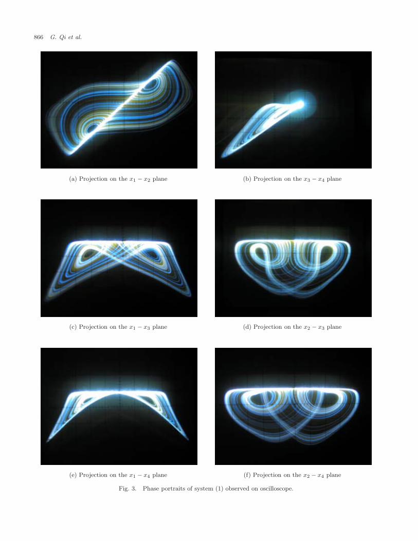
the lower attractor is omitted, and the orbits of bothupper and lower attractors cannot move into theiropposite regions. When e = ±7, a new periodicorbit appears. According to the geometric locationsof the attractors, they are called anti-diagonal peri-odic orbit with e = 7 around S1,4, and a diagonalperiodic orbit with e = −7 around S2,3.

Many simulations show that both the diagonaland the anti-diagonal periodic orbits move aroundthe two equilibria, which form a short diagonal line,as mentioned above.

It is significant that both the periodic orbits cantraverse the hyperplanes x3 = 0 and x4 = 0, and donot rely on initial values. With parameters beinggradually varied, the periodic orbits will evolve intochaos. In some parameters range, if the orbit of

system (16) not only travels between S1,4 or S2,3,but also moves around S1,2 and S3,4, then system(16) will generate a real four-wing attractor. Forexample, with a = 50, b = 4.2, c = 13, d = 20, e =7, system (16) is in chaotic mode with the maximumLyapunov exponent equal to 0.69066, as shown inFigs. 9(a) and 9(b). Comparing them with Figs. 8(c)and 8(d), one sees that the anti-diagonal periodicorbit has evolved into chaos, and some orbits beginto move among equilibria S1,2 and S3,4, graduallyforming a four-wing chaotic attractor. With furtherchanges of parameters, till a = 50, b = 7, c = 13,d = 20, e = 7, a real four-wing chaotic attractor isclearly formed, as shown in Figs. 10(a)–10(h). It isnotable that there exist many anti-diagonal flowsfreely running around S1,4, S1,2 and S3,4, which

−20 −10 0 10 20−5

0

5

10

15

x1

x3

(a) Projection on the x1 − x3 plane, e = 0

−15 −10 −5 0 5 10 15−5

0

5

10

15

x2

x4

(b) Projection on the x2 − x4 plane, e = 0

−10 −5 0 5 10−6

−4

−2

0

2

4

6

x1

x3

(c) Projection on the x1 − x3 plane, e = 7

−6 −4 −2 0 2 4 6−6

−4

−2

0

2

4

6

x2

x4

(d) Projection on the x2 − x4 plane, e = 7

Fig. 8. Upper chaotic attractor, anti-diagonal periodic orbit, and diagonal periodic orbit of system (16), with a = 50, b = 4,c = 13, d = 20, and e = 0, e = 7, e = −7, respectively.

874 G. Qi et al.

−10 −5 0 5 10−6

−4

−2

0

2

4

6

x1

x3

(e) Projection on the x1 − x3 plane, e = −7

−6 −4 −2 0 2 4 6−6

−4

−2

0

2

4

6

x2

x4

(f) Projection on the x2 − x4 plane, e = −7


−15 −10 −5 0 5 10 15−15

−10

−5

0

5

10

15

x1

x3


−15 −10 −5 0 5 10 15−15

−10

−5

0

5

10

15

x2

x4


Fig. 9. The evolution process from diagonal periodic orbit to four-wing chaotic attractor: a = 50, b = 4.2, c = 13, d = 20,e = 7.

are different from the flows of system (1) shown inFig. 1, which are tangent to x3 = 0 or x4 = 0. Thediagonal and anti-diagonal orbits play an importantrole in forming the real four-wing attractor, sincethey connect the upper and the lower attractorstogether.

4.4. Circuit implement of thefour-wing attractor

Another electronic circuit has been designed to real-ize system (16) with parameters a = 50, b = 7,c = 13, d = 20, e = 7, as shown in Fig. 2, includingR34 in the red dashed block of the fourth channelto add the linear term into the fourth equation of

system (16). From the relation representation (15),one has R7 = 20 K, R10 = 50 K, R14 = 14.29 K,R24 = 0.769 K, R28 = 5K, R34 = 14.29 K. Theother resistors and capacitors are unchanged.

Experimental observations on the oscilloscopeare shown in Figs. 11(a)–11(f). A four-wing chaoticattractor can be clearly seen, which is identicalto the simulation results shown in Figs. 10(a) and10(f).

Remark 4.5. According to the above theoreticalanalysis, numerical observations, and analog circuitexperiments, it has been confirmed that system (16)has a real four-wing attractor.


−20 −10 0 10 20−20

−15

−10

−5

0

5

10

15

20

x1

x2


−20 −10 0 10 20−20

−15

−10

−5

0

5

10

15

20

x3

x4


−20 −10 0 10 20−20

15

−10

−5

0

5

10

15

20

x1

x3


−20 −10 0 10 20−20

−15

−10

−5

0

5

10

15

20

x2

x3


−20 −10 0 10 20−20

−15

−10

−5

0

5

10

15

20

x1

x4

(e) Projection on the x1 − x4 plane

−20 −10 0 10 20−20

−15

−10

−5

0

5

10

15

20

x2

x4

(f) Projection on the x2 − x4 plane

Fig. 10. The real four-wing chaotic attractor of system (16): a = 50, b = 7, c = 13, d = 20, e = 7.

876 G. Qi et al.

−20−10

010

20

2010

0−10

−20−20

−10

0

10

20

x1x2

x3

(g) 3-D view in the x1 − x2 − x3 space (h) 3-D view in the x2 − x3 − x4 plane


(a) Projection on the x1 − x2 plane (b) Projection on the x3 − x4 plane

(c) Projection on the x1 − x3 plane (d) Projection on the x2 − x3 plane

Fig. 11. The four-wing chaotic attractor observed on the oscilloscope.


(e) Projection on the x1 − x4 plane (f) Projection on the x2 − x4 plane


4.5. Bifurcation analysis of thefour-wing attractor

In the following, the four-wing attractor is furtherinvestigated by means of bifurcation and Lyapunovexponent spectrum analyses.

4.5.1. Fix a = 50, c = 13, d = 20, e = 7, andvary parameter b

Figure 12 shows the Lyapunov exponent spectrumwith b ∈ [0, 20], where the Lyapunov exponents areordered by magnitude: λ1 > λ2 > λ3 > λ4.

It is notable that when b ∈ [0, 2.5], the max-imum exponent λ1 is negative, so the systemhas sinks at some equilibria. By calculation with

0 2 4 6 8 10 12 14 16 18 20−60

−50

−40

−30

−20

−10

0

10

20

b

Lyap

unov

exp

onen

ts

λ1

λ2

λ3

λ4

Fig. 12. The Lyapunov exponent spectrum versus b.

b = 1.5, it was found that S1,4 are stable fociwith eigenvalues [−51.25,−1.40 + 12.83i,−1.40 −12.83i,−27.45], but the other equilibria are sad-dle points, leading the orbits to converge to S1

or S4 depending on the initial values, as shown inFig. 13(a).

When b ∈ [2.5, 4], the maximum exponent λ1 =0, so the system displays periodic orbits, as shownin Figs. 8(c) and 8(d). When b > 4, the systemhas a four-wing attractor. With b increasing, onone side the equilibria S1,2,3,4 and S5,6,7,8 graduallyform some rectangles, namely, the destroyed sym-metries are revived, so the attractive forces of theequilibria, including S1,2 and S3,4, are revived, asshown in Figs. 13(b) and 13(c); on the other hand,the effect of the control term ex2 gradually reduces,so the attractive forces of equilibria S1,4 and S2,3

gradually decrease, as shown in Figs. 13(b) and13(c). In the end, the system displays two coexistingdouble-wing chaotic attractors: an upper one and alower one, as shown in Fig. 13(d).

4.5.2. Fix a = 50, b = 7, c = 13, d = 20, andvary parameter e

According to Remarks 4.3 and 4.4, the orbit ofsystem (16) has some symmetries with respect toparameter e; therefore, one only needs to discussthe evolution process in the range e < 0. Figure 14shows the bifurcation diagram of state x3 at equilib-rium S2, where two blue lines indicate the locationsof equlibira S2 and S4 with e being varied. It is clearthat S2 and S4 are not symmetric with respect tox3 = 0. As |e| becomes larger, the nonsymmetric

878 G. Qi et al.

−6 −4 −2 0 2 4 6−4

−3

−2

−1

0

1

2

3

4

x1

x3

(a) The orbit convergent to S1 or S4: b = 1.5

−30 −20 −10 0 10 20 30

−20

−10

0

10

20

x1

x3

(b) A four-wing chaotic attractor: b = 12

−30 −20 −10 0 10 20 30−30

−20

−10

0

10

20

30

x1

x3

(c) A four-wing chaotic attractor: b = 17

−30 −20 −10 0 10 20 30−30

−20

−10

0

10

20

30

x1

x3

(d) Two coexisting double-wing chaotic attractors: b = 22

Fig. 13. The evolution process: from sink, to four-wing chaotic attractor, to two double-wing chaotic attractors.

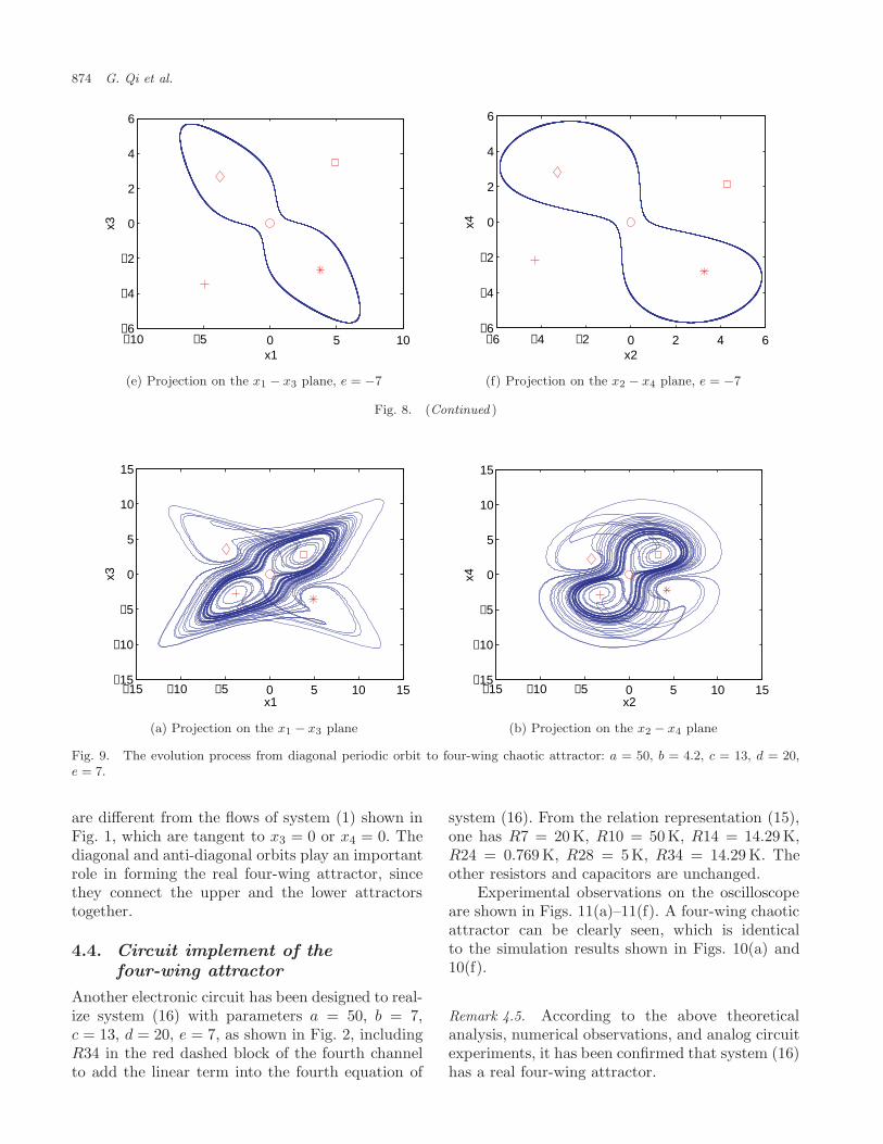
property becomes clearer. Figure 15 shows the cor-responding Lyapunov exponent spectrum.

Both Figs. 14 and 15 show that when e ∈[−40,−35.15], system (16) displays a periodic orbit.With the parameter being varied, the orbit evolvesfrom just one of S2,3 (see Figs. 16(a) and 16(b)) towandering among the equilibria-pair (see Figs. 16(c)and 16(d)), where this kind of evolution processhowever cannot be seen in the bifurcation diagram,Fig. 14, where only bifurcations at equilibrium S2

are plotted.With e > −35.15, the system suddenly goes

into a diagonal double-wing chaotic attractor, asshown in Figs. 16(e) and 16(f), and there area few trajectories moving among S1,2 and S3,4.With e increasing, the system rapidly becomesa real four-wing chaotic attractor, as shown in

Figs. 16(g)–16(j). These evolution processes furtherdemonstrate that it is just the flows of the diagonalattractor that connect the upper attractor with thelower one to form a whole attractor with four-wings.

Remark 4.6. If one introduces a linear feedback con-trol term to the third equation of system (1), suchas fx1 or fx2, where f is a constant parameter,then symmetries and the distribution of equilib-ria of the controlled system (1) will be changedaccordingly. Similarly, the controlled system willcreate a new chaotic mode, such as diagonal oranti-diagonal attractors and a four-wing chaoticattractor.

Since the results are quite similar, this case willnot be further pursued here in this paper.


Fig. 14. The bifurcation diagram of x3 versus parameter e.

−40 −35 −30 −25 −20 −15 −10 −5 0−60

−50

−40

−30

−20

−10

0

10

e

Lyap

unov

exp

onen

ts

λ1

λ2

λ3

λ4

Fig. 15. The Lyapunov exponent spectrum versus e.

5. System Under Sign-SwitchingControl

Recall Remark 4.3, which implies that if one drawssimultaneously the orbits of system (16) with e and−e on one figure, then it can be seen that thesetwo orbits are symmetric with respect to the x1-axis on the coordinate planes x1 − x3 and x1 − x4,and they are also symmetric with respect to thex2-axis on planes x2 − x3, x2 − x4, as can be fur-ther verified by comparing Figs. 8(c) and 8(d) withFigs. 8(e) and 8(f), and comparing Figs. 10(c) and10(f) with Figs. 16(i) and 16(j). Therefore, here weconsider changing the constant control parameter ein system (16), and replace it by a sign-switching

function. The system under consideration is

x1 = a(x2 − x1) + x2x3x4

x2 = b(x1 + x2) − x1x3x4

x3 = −cx3 + x1x2x4

x4 = −dx4 + e(t)x2 + x1x2x3

(30)

where e(t) = e sign(sin wt) is the sign-switchingcontrol function.

Notice that system (30) contains smooth cubicnonlinearities, which is different from the gener-alized Chua’s circuit, and contains also one sign-switching function which changes sign periodicallybetween e and −e. This leads all equilibria to switchbetween S0,...,9(e) and S0,...,9(−e), and then leadsthe system orbit to switch between those of system(16) with e and −e, respectively.

Some new phenomena are found, as furtherdiscussed below.

Firstly, take b = 1, and fix a = 50, c = 13,d = 20, ω = 0.4(rad/sec), e = 7 in system (30). Theresults are shown in Figs. 18(a) and 18(b), in whichthe red trajectory and the blue one start from dif-ferent initial values. One can see two new coexistingdouble-wing attractors: one on the left and anotheron the right sides.

For system (16) with these parameters, as canbe seen in Fig. 12, the maximum Lyapunov expo-nent is negative, which means that any orbit of sys-tem (16) converges to a sink. In fact, the eigenvalues

880 G. Qi et al.

−10 −5 0 5 10−8

−6

−4

−2

0

2

4

6

8

x1

x3

(a) Projection on the x1 − x3 plane, e = −38

−6 −4 −2 0 2 4 6−8

−6

−4

−2

0

2

4

6

8

x2

x4

(b) Projection on the x2 − x4 plane, e = −38

−10 −5 0 5 10−8

−6

−4

−2

0

2

4

6

8

x1

x3

(c) Projection on the x1 − x3 plane, e = −36

−6 −4 −2 0 2 4 6−8

−6

−4

−2

0

2

4

6

8

x2

x4

(d) Projection on the x2 − x4 plane, e = −36

−20 −10 0 10 20−15

−10

−5

0

5

10

15

x1

x3

(e) Projection on the x1 − x3 plane, e = −34 (f) Projection on the x2 − x4 plane, e = −34

Fig. 16. The evolution process of system (16) with e being varied.


(g) Projection on the x1 − x3 plane, e = −15 (h) Projection on the x2 − x4 plane, e = −15

(i) Projection on the x1 − x3 plane, e = −7

−20 −10 0 10 20−20

−15

−10

−5

0

5

10

15

20

x2

x4

(j) Projection on the x2 − x4 plane, e = −7


of S1,4(e) and S2,3(−e), with e = 7, are

� = [−50.78,−2.29 + 10.13i,

−2.29 − 10.13i,−26.64]T (31)

and the other equilibria are saddle. This means thatthe orbit of system (16) with e converges to oneof S1(e) and S4(e), but the orbit of system (16)with −e converges to one of S2(−e) and S3(−e).The distribution of the system equilibria is shown inFig. 17, where the red symbols “o”, “�”, “♦”, “∗”,“+” denote S0,1,2,3,4(e), respectively, and the bluesymbols “�”, “♦”, “∗”, “+” denote S1,2,3,4(−e),respectively.

In system (30), since the sign of e(t) switchesbetween e and −e (e = 7) with frequency ω =0.4(rad/sec), the system equilibria switch between

S0,...,9(e) and S0,...,9(−e). Before switching, if ini-tial value is taken from the attraction domain ofS1(e), the trajectory of system (30) will convergeto S1(e)(red “�” in Fig. 17), but after switching,the trajectory escapes from the attraction domain ofS1(e) and goes into one of the two sinks, S2(−e) andS3(−e), (blue “♦” and “∗” in Fig. 17), dependingon which attraction domain the trajectory was in.

There are three cases to be discussed here.

(i) If the trajectory goes into the attractiondomain of S3(−e), it will wander betweenS1(e) and S3(−e) over and over again. Then,the right attractor is formed. Similarly, the leftattractor moves around S4(e) and S2(−e). For

882 G. Qi et al.

−6 −4 −2 0 2 4 6−3

−2

−1

0

1

2

3

x1

x3

(a) Projection on x1 − x3

−6 −4 −2 0 2 4 6−2

−1.5

−1

−0.5

0

0.5

1

1.5

2

x2

x4

(b) Projection on x2 − x4

Fig. 17. Distribution of the equilibria of system (16): a = 50, b = 1, c = 13, d = 20, e = ±7.

−5 0 5−3

−2

−1

0

1

2

3

x1

x3

(a) Projection on x1 − x3, b = 1

−5 0 5−3

−2

−1

0

1

2

3

x2

x4

(b) Projection on x2 − x4, b = 1

−8 −4 0 4 8−5

0

5

x1

x3

(c) Projection on x1 − x3, b = 1.9

−6 −4 −2 0 2 4 6−5

0

5

x2

x4

(d) Projection on x2 − x4, b = 1.9

Fig. 18. Two coexisting double-wing attractors: left attractor and right attractor of system (30): a = 50, c = 13, d = 20,e = 7, ω = 0.4 (rad/sec).


−10 −5 0 5 10−6

−4

−2

0

2

4

6

x1

x3

−8 −4 0 4 8−6

−4

−2

0

2

4

6

x2

x4

Fig. 19. Two existing double-wing attractors of system (30): a = 50, b = 2.1, c = 13, d = 20, e = 7, ω = 0.4 (rad/sec).

example, with b = 1 and b = 1.9, Figs. 18(a)–18(d) show the resulting left and right attrac-tors, respectively.

(ii) If the trajectory goes into the attractiondomain of S2(−e), it will wander between S1(e)and S2(−e), and then the upper attractor isformed (red orbit in Figs. 18(e) and 18(f)).Similarly, the lower attractor can be formed,which moves between S4(e) and S3(−e) (blueorbit in Figs. 18(e) and 18(f)).

It is notable that different values of b yielddifferent oscillatory amplitudes and conver-gence speeds to the sinks, further influencingthe tendency of the system trajectories and theshape of the attractors.

(iii) If the varying parameter of system (30) is suit-ably chosen, the system trajectory will moveamong four equilibria, forming a new four-wing attractor via switching this parameter.For example, fix a = 50, c = 20, d = 20,e = 7, and set b = 2.5, ω = 0.4, or b = 2.2,ω = 1, respectively. Then, a four-wing attrac-tor is generated, with a 3D view shown inFigs. 20(a)–20(d).

Notice from Fig. 12 that with b < 2.5, the orbitof system (16) converges to one sink, while when2.5 ≤ b < 4, it becomes a periodic orbit. So, theattractors shown in Figs. 18, 19, 20(c)–20(d) arenot chaotic attractors.

Note also that system (30) can actually dis-play a four-wing chaotic attractor as long as system(16) is in chaotic mode within some parameters’range. For example, with b = 4.5, ω = 0.4, andother parameters unchanged, according to Fig. 12,

the maximum Lyapunov exponent is positive. Ithas been shown above, system (16) with e = ±7can display a double-wing anti-diagonal chaoticattractor and a diagonal chaotic attractor, respec-tively. Figures 20(e) and 20(f) show a four-wingchaotic attractor of system (30), which is generatedby switching between these anti-diagonal chaoticand diagonal chaotic attractors.

As seen above, by introducing a sign-switchingfunction in the linear state-feedback control term,the trajectory of system (16) can switch betweentwo sinks, or escape from a sink to another, overand over again, thereby generating left and rightdouble-wing attractors.

6. Conclusions

In this paper, some basic dynamical behaviorsand the compound structure of the new four-dimensional chaotic system found in [Qi et al.,2005a] have been further investigated. In additionto some interesting symmetries, a four-wing chaoticattractor is first observed numerically, and thenproven both theoretically and experimentally to bea numerical artifact, which actually consists of twocoexisting double-wing chaotic attractors and thesetwo double-wing attractors are arbitrarily close toeach other but never truly connected together. Fur-ther analysis has shown that this artifact is pro-duced due to three reasons: distribution of systemequilibria, location of system manifolds, and errorsof numerical computations. To that end, by addinga simple linear term to the system, considered asa linear sate-feedback control input, a real four-wing attractor was generated. With the extra linearterm, the system has nine equilibria of five different

884 G. Qi et al.

(a) 3-D view in x4 − x1 − x2 space, b = 2.5, ω = 0.4 (b) 3-D view in x1 − x3 − x4 space, b = 2.5, ω = 0.4

(c) 3-D view in x1 − x2 − x4 space, b = 2.5, ω = 1 (d) 3-D view in x1 − x3 − x4 space, b = 2.5, ω = 1

(e) 3-D view in x1 − x2 − x3, b = 4.5, ω = 0.4 (f) 3-D view in x2 − x3 − x4, b = 4.5, ω = 0.4

Fig. 20. Four-wing attractor generated by sign-switching: a = 50, c = 13, d = 20, e = 7.

types, classified according to their linearized char-acteristics, and has symmetries as well as similar-ities, which have all been analyzed in the paper.In summary, a relatively simple four-dimensionalautonomous system with a real four-wing chaotic

attractor has been coined, and circuit implemen-tation has been implemented which further verifiesthat this four-wing chaotic attractor is real.

In this paper, the evolution process from twocoexisting up-down attractors to two diagonally or


anti-diagonally located periodic orbits, and even-tually to merge as a real four-wing attractor, hasalso been investigated by means of bifurcation andLyapunov exponent analyses. Finally, it has beenshown that under a sign-switching control, the sys-tem orbit can be manipulated to switch between twosinks, thereby generating a left and a right double-wing attractor, which eventually also lead to a trulysingle four-wing attractor.

It has been realized that generating a newchaotic system by suitable state-feedback control isan important concept and powerful technique, con-sidered as an effective chaotification method. In theendeavour of chaotification, this paper has addeda new model to the recently found large family ofnew chaotic systems created by chaotification, suchas Chen system [Chen & Ueta, 1999], Lu system[Lu & Chen, 2002], and generalized Lorenz canoni-cal form [Celikovsky & Chen, 2002].

Acknowledgment

This work was supported by a grant from theResearch Grants Council of the Hong Kong SpecialAdministrative Region, China [Project No. CityU1115/03E].

References

Baghious, E. H. & Jarry, P. [1993] “Lorenz attractor fromdifferential equations with piecewise-linear terms,”Int. J. Bifurcation and Chaos 3, 201–210.

Celikovsky, S. & Chen, G. [2002] “On a generalizedLorenz canonical form of chaotic systems,” Int. J.Bifurcation and Chaos 12, 1789–1812.

Chen, G. & Ueta, T. [1999] “Yet another chaotic attrac-tor,” Int. J. Bifurcation and Chaos 9, 465–1466.

Chen, G. & Lu, J. [2003] Dynamical Analysis, Controland Synchronization of the Generalized Lorenz Sys-tems Family (in Chinese) (Science Press, Beijing).

Chen, G. & Yu, X. [2003] Chaos Control: Theory andApplications (Springer-Verlag, Berlin).

Chua, L. O., Komuro, M. & Matsumoto, T. [1986] “Thedouble scroll family,” IEEE Trans. Circuits Syst.-I33, 1072–1118.

Chua, L. O. & Roska, T. [1993] “The CNN paradigm,”IEEE Trans. Circuits Syst.-I 40, 147–156.

Elwakil, A. S. & Kennedy, M. P. [2000] “Systematic real-ization of a class of hysteresis chaotic oscillators,” Int.J. Circuit Th. Appl. 28, 319–334.

Elwakil, A. S. & Kennedy, M. P. [2001] “Construction ofclasses of circuit-independent chaotic oscillators usingpassive-only nonlinear devices,” IEEE Trans. CircuitsSyst.-I 48, 289–307.

Elwakil, A. S., Ozogus, S. & Kennedy, M. P. [2002] “Cre-ation of a complex butterfly attractor using a novelLorenz-type system,” IEEE Trans. Circuits Syst.-I49, 527–530.

Han, F., Yu, X., Lu, J., Chen & Feng, Y. [2005] “Gen-erating multiscroll chaotic attractors via a linearsecond-order hysteresis system,” Dyn. Contin. Discr.Impu. Syst. Series B: Appl. Algorith. 12, 95–110.

Liu, W. & Chen, G. [2003] “A new chaotic system and itsgeneration,” Int. J. Bifurcation and Chaos 13, 261–267.

Liu, W. & Chen, G. [2004] “Can a three-dimensionalsmooth autonomous quadratic chaotic system gener-ate a single four-scroll attractor?” Int. J. Bifurcationand Chaos 14, 1395–1403.

Lu, J. & Chen, G. [2002] “A new chaotic attractorcoined,” Int. J. Bifurcation and Chaos 12, 659–661.

Lu, J., Yu, X. & Chen, G. [2003] “Generating chaoticattractors with multiple merged basins of attraction:A switching piecewise-linear control approach,” IEEETrans. Circuits Syst.-I 50, 198–207.

Lu, J., Chen, G. & Cheng, D. [2004a] “A new chaoticsystem and beyond: The generalized Lorenz-like sys-tem,” Int. J. Bifurcation and Chaos 14, 1507–1537.

Lu, J., Chen, G. & Yu, X. [2004b] “Design and analysis ofmultiscroll chaotic attractors from saturated functionseries,” IEEE Trans. Circuits Syst.-I 51, 2476–2490.

Lu, J., Han, F., Yu, X. & Chen, G. [2004c] “Generating3-D multiscroll chaotic attractors: A hysteresis seriesswitching method,” Automatica 40, 1677–1877.

Ozoguz, S., Elwakil, A. S. & Salama, K. N. [2002]“n-scroll chaos generator using nonlinear transcon-ductor,” Electron. Lett. 38, 685–686.

Qi, G., Du, S., Chen, G., Chen, Z. & Yuan, Z. [2005a]“On a 4-dimensional chaotic system,” Chaos Solit.Fract. 23, 1671–1682.

Sparrow, C. [1982] The Lorenz Equations: Bifurcations,Chaos, and Strange Attractors (Springer-Verlag, NY).

Suykens, J. A. K. & Vandewalle, J. [1993] “Generationof n-double scrolls (n = 1; 2; 3; 4; . . .),” IEEE Trans.Circuits Syst.-I 40, 861–867.

Suykens, J. A. K. & Chua, L. O. [1997] “n-double scrollhypercubes in 1-D CNNs,” Int. J. Bifurcation andChaos 7, 1873–1885.

Tang, K. S., Zhong, G. Q., Chen, G. & Man, K. F. [2001]“Generation of n-scroll attractors via sine function,”IEEE Trans. Circuits Syst.-I 48, 1369–1372.

Vanecek, A. & Celikovsky, S. [1996] Control Systems:From Linear Analysis to Synthesis of Chaos(Prentice-Hall, London).

Yalcin, M. E., Ozoguz, S., Suykens, J. A. K. &Vandewalle, J. [2001a] “n-scroll chaos generators: Asimple circuit model,” Electron. Lett. 37, 147–148.

Yalcin, M. E., Suykens, J. A. K., Vandewalle, J. &Ozoguz, S. [2002b] “Families of scroll grid attractors,”Int. J. Bifurcation and Chaos 12, 23–41.

Four-wing attractors from pseudo to real

Documents

Transcript of Four-wing attractors from pseudo to real