Deterministic-random separation in nonstationary regime

HAL Id: hal-01285390https://hal.archives-ouvertes.fr/hal-01285390

Submitted on 3 Sep 2021

HAL is a multi-disciplinary open accessarchive for the deposit and dissemination of sci-entific research documents, whether they are pub-lished or not. The documents may come fromteaching and research institutions in France orabroad, or from public or private research centers.

L’archive ouverte pluridisciplinaire HAL, estdestinée au dépôt et à la diffusion de documentsscientifiques de niveau recherche, publiés ou non,émanant des établissements d’enseignement et derecherche français ou étrangers, des laboratoirespublics ou privés.

Deterministic-random separation in nonstationaryregime

Dany Abboud, Jérôme Antoni, Sophie Sieg-Zieba, Mario Eltabach

To cite this version:Dany Abboud, Jérôme Antoni, Sophie Sieg-Zieba, Mario Eltabach. Deterministic-random separationin nonstationary regime. Journal of Sound and Vibration, Elsevier, 2016, Journal of Sound andVibration, 362, pp.305-326. �10.1016/j.jsv.2015.09.029�. �hal-01285390�

https://hal.archives-ouvertes.fr/hal-01285390

https://hal.archives-ouvertes.fr

Contents lists available at ScienceDirect

Journal of Sound and Vibration

Journal of Sound and Vibration 362 (2016) 305–326

http://d0022-46

Abbreinvariandensity

n CorrE-m

sophie.s

journal homepage: www.elsevier.com/locate/jsvi

Deterministic-random separation in nonstationary regime

D. Abboud a,b,n, J. Antoni a, S. Sieg-Zieba b, M. Eltabach b

a Laboratoire Vibrations Acoustique (LVA), Université de Lyon (INSA), F-69621 Villeurbanne Cedex, Franceb Technical Center of Mechanical Industries (CETIM), CS 80067, 60304 Senlis Cedex, France

a r t i c l e i n f o

Article history:Received 4 November 2014Received in revised form15 September 2015Accepted 18 September 2015
Handling Editor: K. Shin
vibration-based diagnosis in order to discriminate useful information from masking noise.

Available online 31 October 2015

x.doi.org/10.1016/j.jsv.2015.09.0290X/& 2015 Elsevier Ltd. All rights reserved.

viations: CS, cyclostationary; CS1, first-ordt; CNS, cyclo-non-stationary; DRS, determinestimation; SES, squared envelope spectrumesponding author.ail addresses: [email protected], [email protected] (S. Sieg-Zieba), mario.elta

a b s t r a c t

In rotating machinery vibration analysis, the synchronous average is perhaps the mostwidely used technique for extracting periodic components. Periodic components aretypically related to gear vibrations, misalignments, unbalances, blade rotations, recipro-cating forces, etc. Their separation from other random components is essential in

However, synchronous averaging theoretically requires the machine to operate understationary regime (i.e. the related vibration signals are cyclostationary) and is otherwisejeopardized by the presence of amplitude and phase modulations. A first object of thispaper is to investigate the nature of the nonstationarity induced by the response of alinear time-invariant system subjected to speed varying excitation. For this purpose, theconcept of a cyclo-non-stationary signal is introduced, which extends the class ofcyclostationary signals to speed-varying regimes. Next, a “generalized synchronousaverage’’ is designed to extract the deterministic part of a cyclo-non-stationary vibrationsignal—i.e. the analog of the periodic part of a cyclostationary signal. Two estimators ofthe GSA have been proposed. The first one returns the synchronous average of the signalat predefined discrete operating speeds. A brief statistical study of it is performed, aimingto provide the user with confidence intervals that reflect the "quality" of the estimatoraccording to the SNR and the estimated speed. The second estimator returns a smoothedversion of the former by enforcing continuity over the speed axis. It helps to reconstructthe deterministic component by tracking a specific trajectory dictated by the speed profile(assumed to be known a priori).The proposed method is validated first on synthetic sig-nals and then on actual industrial signals. The usefulness of the approach is demonstratedon envelope-based diagnosis of bearings in variable-speed operation.

& 2015 Elsevier Ltd. All rights reserved.

1. Introduction

In most mechanical systems, gears and rolling-element bearings constitute the core elements of the power transmissionchain. Therefore, their diagnosis is critical to ensure the security of the equipment and avoid possible breakdowns in the

er cyclostationary; CS2, second-order cyclostationary; SA, synchronous average; LTI, linear time-istic random separation; GSA, generalized synchronous average; dof, degree-of-freedom; KDE, kernel

[email protected], [email protected] (D. Abboud), [email protected] (J. Antoni),[email protected] (M. Eltabach).

www.sciencedirect.com/science/journal/0022460X

www.elsevier.com/locate/jsvi

http://dx.doi.org/10.1016/j.jsv.2015.09.029



http://crossmark.crossref.org/dialog/?doi=10.1016/j.jsv.2015.09.029&domain=pdf



mailto:[email protected]







Nomenclature

card Κr� �

number of cycles belonging to regime rΚr set of cycle indices belonging to regime rmY ðθÞ SA of YmY ðθ;ωÞ GSA of YmY θ

� �GSA trajectory tracked for a given speed pro-file ω¼ω θ

� �bmY ðθ;ωrÞraw estimator of the GSA of Y at ωrbmY ðθ;ωÞ smoothed estimator of the GSA of YPY ðθ;ωrÞ mean instantaneous power of Y at ωr

t time variableδω speed resolutionΔω speed varying marginE �f g ensemble averaging operatorE �jAf g ensemble average operator conditioned to

event Aθ angle variableθ angular location in the cycle: θϵ 0;Θ

� �Θ angular periodωr central angular frequency at regime r

D. Abboud et al. / Journal of Sound and Vibration 362 (2016) 305–326306

system. Interestingly, it was shown that these components—when operating under constant regime—produce symptomaticcyclostationary (CS) vibrations that can be identified and characterized by dedicated tools [1]. Specifically, gears are likely togenerate first-order cyclostationary (CS1) vibrations characterized by a periodic mean, whereas rolling-element bearingsgenerate second-order cyclostationary (CS2) vibrations characterized by a periodic autocovariance function. The former aredeterministic in nature, whilst the latter are random. Their separation is of high practical importance for differentialdiagnosis [2–4].

In this context, the synchronous average (SA) is a powerful tool for extracting periodic components [5,6]. Based on priorknowledge of the desired component, it consists of segmenting the temporal signal into blocks of length equal to the signalperiod and averaging them together to extract the periodic waveform. The “residual signal”—which constitutes the randompart—is then obtained by subtracting the estimated periodic part from the original signal. The principle of the SA assumesthe periodic waveform to be stable in time, which in turn requires a constant speed. However, in practice, such a condition isdifficult to obtain: the operating speed often undergoes some fluctuations which are likely to jeopardize the effectiveness ofthe SA, even if very low. Since repetitive patterns in rotating machines are intrinsically locked to specific angular positions, itthus makes sense to synchronize the SA with respect to angle rather than to time. This problem has found several practicalsolutions such as angular sampling or resampling (also known as “computed order tracking” [7]): whereas the formerdirectly acquires the signal at constant angular intervals, the latter uses a tachometer to resample the time signal at constantangular increments by interpolation [8,9]. In this case, the cyclostationary property holds in the angle domain and, con-sequently, the SA is applied on the (resampled) signal. Incidentally, this facilitates the averaging operation since eachangular period then comprises the same (whole) number of angular increments. Nevertheless, the change from a temporalto an angular variable raises issues about the actual nature of cyclostationarity of rotating machine signals. This was forinstance addressed in Ref. [10] where the authors explored the concept of angle-CS signals and provided the conditions of itsequivalence with the time-CS.

In the case of high speed fluctuations, signals are subjected to significant distortions that jeopardize the effectiveness ofthe SA. These distortions are basically introduced by (i) variations of the machine power intake and (ii) the effect of lineartime-invariant (LTI) transfers. Whereas the first effect essentially results in amplitude modulation, the second one alsoinduces phase modulation. The latter phenomenon was originally inspected in Ref. [11], before being revisited in Ref. [12]through a comprehensive theoretical analysis. Non-periodic modulations obviously invalidate the (angle-) CS assumptionand call for a more general description of nonstationary signals. In accordance, “cyclo-non-stationarity” (CNS), a new classrecently introduced in Ref. [13], appears to be a good candidate to describe speed-varying signals: it enfolds highly non-stationary signals undergoing long-term structural changes in their properties, yet preserving at the same time short-termcyclic rhythms locked to the angular evolution.

The consideration of CNS signals requires the revision of existing CS tools and in particular of the SA. In order toaccommodate the SA with the phase blur resulting from the transmission path effect, Stander and Heyns [11] proposed anenhanced version coined “phase domain averaging”—comprising a phase correction of the cycles before the averagingoperation. The phase information was returned by Hilbert demodulation of a high-energy harmonic (such as a meshingorder) of the resampled acceleration signal. Later, a simpler variant was provided in Ref. [14], coined the “improved syn-chronous average”, which consists in resampling the signal with a virtual tachometer signal synthesized via the demodu-lated phase. This work was inspired from Ref. [9] which introduced a technique to perform angular resampling using theacceleration signal of a gearbox operating under limited speed fluctuation.

Recently, the same technique was used in Ref. [12] to identify the optimal demodulation band for deterministic/randomseparation (DRS) in speed varying conditions. Moreover, the authors in Ref. [15] provided a parametric approach in anattempt to generalize the SA to the CNS case. Using Hilbert space representation, they decomposed the deterministiccomponents on to a set of periodic functions multiplied by speed-dependent functions apt to capture long-term evolutionover consecutive cycles. Yet, their method carries the general disadvantages of parametric approaches, namely, the criticaldependence on the basis order. Another attempt was made recently in Ref. [13] where the aim was to remove the deter-ministic part of the vibrations produced by an internal combustion engine in runup regimes. Assuming a first-order Markov

D. Abboud et al. / Journal of Sound and Vibration 362 (2016) 305–326 307

dependence of the CNS signal, the authors introduced an operator—coined the “cyclic difference”—based on subtractingeach cycle from the previous one in the resampled signal. Despite the good compliance of this method for the particularaddressed application, it suffers from high variability in the more general setting.

The principal object of this paper is to provide a novel operator, coined the “generalized synchronous average” (GSA),which happens to be an extension of the classical SA to the CNS case, with the aim of enhancing DRS in variable regime. It isassumed that the rotational speed is precisely known; its estimation is beyond the scope of this paper and may be found inreferences such as [16–25]. This paper is organized as follows: Section 2 states the problem with a particular attention toformulating the transmission path effect from a CNS view. Section 3 introduces the GSA operator, two dedicated estimatorsof it and a statistical study in order to evaluate the estimator quality according to the SNR and the estimated speed. Section 4validates the effectiveness of the GSA on numerical signals and Section 5 on actual industrial signals. Eventually, in light ofthe obtained results, the paper is sealed with a general conclusion in Section 6.

2. Problem statement

This section starts with a brief review of the SA. Then, the transmission path effect is qualitatively addressed with a linkmade with CNS.

2.1. Synchronous average: a brief review

The synchronous average (SA)—widely termed as the time synchronous average [26]—is an efficient technique for theextraction of periodic waveforms from a noisy signal. It consists of averaging periodic sections of the signal—known as cycles—assuming a priori knowledge of the period. Under the assumption of cycloergodicity [10], the SA is perhaps the bestcandidate for estimating the mean function of a CS signals. In practice, it is however jeopardized when applied in the time-domain due to existing speed fluctuations or if the signal period is not a multiple of the sampling period. In such cases,angular resampling can be a simple preprocessing solution consisting of expressing the signal in terms of the angularvariable θ of the machine instead of time t. Precisely, let Y θ

� �be an angle-CS signal of cycleΘ (for instanceΘ¼2π); its SA is

then defined as

mY θ�

¼ limM-1

12Mþ1

XMm ¼ �M

Y θþmΘ�

(1)

where 2Mþ1ð Þ stands for the number of averaged cycles and θA 0;Θ� �

for the angular location in the cycle (i.e. θ¼ θ�kΘwith k the greatest integer smaller than θ=Θ). The SA is widely used in vibration analysis of rotating machinery to separatedeterministic waveforms (such as produced by imbalances, misalignments, anisotropic rotors, flexible coupling, gearmeshing and other phenomena) from other competing but random sources.

2.2. Transmission path effect

A primary goal in machine diagnostics is to infer the cause of abnormal vibrations. In most cases, accelerometers areremoted from the sources due to non-intrusion constraints and there exists a transmission path effect characterized by thetransfer function of the structure. In cases where the sensor is intentionally used outside its nominal bandwidth (e.g. as ashock sensor), its transfer function should be considered as well. Consequently, the measured signal is to be interpreted asthe output of an LTI system. This system is characterized by ordinary differential equations in time, independently of theexcitation nature. As a result, the response of the system to a complex exponential temporal waveform is kept unchangedexcept for a phase shift and an amplitude amplification characterized by the system transfer function. In this case, thetransmission path induces maximum amplification and phase shift when the frequency content of the excitation coincideswith a resonance of the transfer function. This also holds true in general for time-CS signals: a LTI system excited by a time-CS signal returns a time-CS output. However, the situation is not the same for angle-CS signals. In the case of large speedvariations, the corresponding response is instantaneously delayed and amplified/attenuated [11] according to the fluctuatingamplitude and frequency content of the input signal. From a temporal view, the system response is the convolution of anonstationary excitation with a LTI transfer function: it is therefore nonstationary as well. Conversely, from an angular pointof view the order content of the excitation remains constant, yet the transfer function becomes angle-varying; therefore, theresponse of the system to an angle-CS excitation is CNS in general, and angle-CS in the particular case of periodic, stationaryor cyclostationary operating speed [10] (see Fig. 1).

The present paper is mainly concerned with angle-CS1 excitation and the related transmission path effect on gearvibrations which jeopardizes the (traditional) SA. The issue can be explained from different but equivalent points of view.First, according to the previous discussion, the system response is no longer angle-CS1, which invalidates the workingassumption of the SA [12]. Alternatively, from an angular point of view, the averaging process over multiple shaft rotationsusually results in an energy loss principally caused by the induced phase blur. Finally, from the order domain point of view,

LTITime-CS(stationary speed case)

Time-CS

LTIAngle-CS(varying speed case)

Angle-CS if the speed is periodic, stationary or CS

CNS elsewhere

Fig. 1. Transmission path effect on cyclostationary excitations.


the SA is equivalent to applying a narrow-band comb filter [27]; yet, the amplitude distortion and the phase blur results inenergy leakage outside the lobes of the comb filter.

In summary, when rotating machines undergo large speed variations, the resulting vibration signals lose their angle-CSproperties; thus, invalidates the application of traditional CS tools such as the SA. The aim of the next section is to char-acterize such signals which preserve repetitive patterns related to the cyclic behavior of the excitation, yet with angle(or time) varying properties.

2.3. Speed dependence

This section introduces the basic model that will serve to define the GSA, which consists of Fourier series whose complexexponentials are function of the angle variable, θ, and the coefficients are only dependent on the speed, ω.

To avoid confusions between angle and time domains, the accent mark “tilde”will refer to the temporal representation ofthe signal. Building on the discussion of Section 2.2, a CNS process can be seen as the response ~Y tð Þ ¼ Y t θ

� �� of a LTI system,

say ~h tð Þ, to an angle-CS excitation

~X tð Þ ¼ X θ tð Þ� �¼Xα

cαX θ tð Þ� �ej2παθ tð Þ

Θ ; (2)

where Θ stands for the angular period of X θ tð Þ� �, cαX θ

� �are mutually (angle-) stationary Fourier coefficients and

θ tð Þ ¼ R t0 ω tð Þdt is the angular position of the reference. In short

~Y tð Þ ¼ ~h tð Þ � ~X tð Þ; (3)

where � stands for the convolution product. In the particular case of constant operating speed (i.e. θ tð Þ ¼ω0t) the responsetakes the particular form

Y θ� �¼X

αcαY θ;ω0� �

ej2παθ tð ÞΘ ¼

Xα

cαX θ� �

A αω0=2� �

ejkΦ αω0=2ð Þ� ej2πα

θΘ; αAZ; (4)

where A fð ÞejkΦ fð Þ ¼H fð Þ is the system frequency response function. Actually, Eq. (4) reflects the pivotal role of the speed notonly on the amplitude, but also on the phase of the system response.

In the case of speed varying excitation, the response would turn into a convolution between an angle-CS excitation andan LTI system, which is less straightforward than Eq. (4) because the input signal would no longer be time-CS in general. Onealternative would be to express the convolution directly in the angular domain, i.e. symbolically

Y θ� �¼ h θ

� � � Y θ� �

; (5)

where h θ� �¼ ~h t θ

� �� would then become angle-varying owing to the nonlinearity of the angle-time relationship. In this

case, the Fourier coefficients of the response at a given instant are principally dependent on the operating speed at thatinstant, as well as past and future instances of the speed profile. This implies that, beside the operating speed, the Fouriercoefficients of the response are also dependent on its higher derivatives at the evaluated instant, i.e.

~Y tð Þ ¼Xα

cαY θ tð Þ;ω tð Þ; _ω tð Þ; €ω tð Þ; :::ω tð Þ…� �ej2πα

θ tð ÞΘ : (6)

Under mild conditions, the dependence on higher derivative orders can be neglected and the variations of bothamplitude and phase are consequently modeled with an explicit dependence on the speed only:

~Y tð Þ ¼Xα

cαY θ tð Þ;ω tð Þ� �ej2πα

θ tð ÞΘ ; (7)

where cαY θ;ω� �

stands for the complex Fourier coefficients having a speed-dependent joint probability density function—i.e.mutually stationary stochastic process for a constant speed ω. The angular representation of a CNS signal can be deduced as

Y θ� �¼X

αcαY θ; ~ω θ

� �� ej2πα

θΘ; (8)

with ~ω θ� �¼ω t θ

� �� . Note that Eq. (7) is perfectly valid for runup regimes (where higher-order derivatives of the speed are

nil) and approximately valid in the case of modest accelerations (i.e. smooth variability of the speed profile). This modelaccounts for changes in the signal structure by introducing a dependency of the Fourier coefficient on speed, while the cyclic


behavior expressed by the complex exponential basis is kept invariant. Therefore, the deterministic part of the systemresponse—which will be lately extracted by the GSA—shows an explicit dependence on the speed and is expressed in theangular domain as

M1Y θ� �¼ E Y θ

� �� ¼Xα

cαY ω θ� ��

ej2παθΘ (9)

where M1Y θ� �

denotes the first-order moment of Y θ� �

, and

cαY ωðθÞ� �¼ E cαY θ;ω� �jω¼ ðθÞ� �

(10)

denotes the expected value of cαY θ;ω� �

conditioned on ω (E �jaf g stands for the expected value of � conditioned to a). Theimportance of this model is to characterize the nonstationarity of the response and to highlight the effect of the speed onthe signal structure. Hence, the consideration of the speed seems to be compulsory for the investigation of the statisticalmoments and, particularly, the mean value. The aim of the next section is to link this model with the CNS class.

2.4. Link with cyclo-non-stationarity

Cyclo-non-stationarity has been recently introduced [13] in an attempt to generalize the CS class to account for possiblelong-term variations in the signal statistics while maintaining short-term cyclic rhythms. The model of Eq. (7) is accordancewith such a definition. Specifically, let Θ be the angular period of the excitation; then, building on Eq. (7), the probabilitydensity function of Y θ

� �,

f Y yð Þ ¼ f Y y;θ;ω�

; (11)

is dependent on both θ and ω (θ is the angular position in the cycle defined in Section 2.1). In particular, the conditionalfirst-order moment reads

M1Y θ;ω�

¼ E Y θ� �jθ=Θ¼ θ;ω θ

� �¼ωn o

¼Xα

cαY ωð Þej2παθΘ; (12)

where ½θ=Θ� stands for the remainder of the fraction θ=Θ, which evidences a dependence of the Fourier coefficients onspeed; this defines a CNS process [28].1

3. The proposed solution

Cyclo-non-stationarity brings to the fore an essential difference between ensemble averaging and angle averaging. Theformer means that averaging is applied over all realizations of a stochastic process, whereas the latter implies that averagingis applied over the time (or angle) variable of a particular realization. In fact, their equivalence is of high practical concern inmost physical applications wherein only one realization is usually available. For CS signals, this is guaranteed by thecycloergodic assumption under which the ensemble average can be replaced by the SA. The primary aim of the presentsection is to introduce an angular operator equivalent to the ensemble average in the CNS case. A consistent estimator is alsoprovided and a brief statistical study is then performed to assess its performance.

3.1. Generalized synchronous average

As previously shown, the statistics of a CNS signal instantaneously change with speed and thus lose their periodicity. As aconsequence, the validity of cyclic averaging is jeopardized. For this reason, angle averaging should be redefined to accountfor the speed dependence and accommodate for the induced changes in the signal. To do so and according to Eq. (11), theidea is to perform the cyclic average on samples pertaining to the same speed. Thus, one can extent the SA to CNS signals byintroducing a more general operator coined the generalized synchronous average (GSA). Given a CNS signal Y θ

� �with angular

period Θ and operating under the speed profile ω θ� �

, the GSA is defined as

mY θ;ω�

¼ limδω-0

limcard Κ

θ;ω

n o-1

1

card Κθ;ω

n oXkAΚ

θ;ω

Y θþkΘ�

; (13)

where δω stands for the speed resolution and Κθ;ω ¼ kAℕ ω� δω2 rω θþkΘ

� oω� δω

2

onstands for the set of samples

located at θ and coinciding with speed values in the interval ω� δω2 ;ω� δω

2

� �. This operator extracts the first-order CNS

(CNS1) “field” corresponding to the deterministic components of a signal for all the existing operating regimes by explicitly

1 In this reference, a CNS process is defined by a Fourier decomposition of nonstationary complex Fourier coefficient. It is worth noting that thisdefinition is rather symbolic since it actually comprises all nonstationary signals, the reason it was not adopted by the authors in the present paper.

CNS1 fieldω

θ

Speed profile ω(θ)

CNS1 Trajectory conditioned to ω(θ)

Θ 2Θ 3Θ 4Θ 5Θ 6Θ 7Θ 8Θ 9Θ …

Fig. 2. Trajectory of a CNS1 signal conditioned to a given speed profile ω(θ). Each horizontal slice in this field associated with a fixed speed value ω

represents a CS process with specific statistics. A CNS process is then a trajectory in this field defined by the speed profile.


accounting for the speed variable. Note that, in the case of constant speed, say ω0, the set Κθ;ω0comprises all the cycles for

all θ and the GSA boils down to the classical SA.Note that the GSA is in general a function of two variables, i.e. angle and speed. Given a particular speed profile ω θ

� �, the

“trajectory” of the CNS1 component of Y θ� �

is thus returned by

mY θ� �¼mY θ¼ θ=Θ;ω¼ω θ

� �� (14)

viewed as a function of θ only—see Fig. 2. Having introduced the GSA, it now remains to propose a consistent estimator thatapplies to finite-length signals. This is addressed in the next section.

3.2. Estimation issues

3.2.1. Raw estimatorThe practical implementation of the GSA faces several difficulties. In particular, the finite length of the signal prevents the

speed resolution to be infinitely narrow and the number of averages to be infinitely large. Furthermore, the cyclic averagingoperation is pointwise, which makes difficult its application in practice. A natural way to overcome this limitation is toassume a stationary behavior of the machine regime in each interval ω�δω=2;ωþδω=2

� �for a given δω40 (i.e. local

stationarity of the speed profile). Stated differently, the signal is supposed to be locally cyclostationary at those speeds. Indetails, the speed profile is divided into a predefined set of speed intervals called regimes defined by their central frequencyωr and the speed resolution δω. Then, each cycle is associated to the regime that is closest to its mean speed value. The rawestimator of the GSA of a finite-length CNS signal Y θ

� �, with angular period Θ and operating speed profile ω θ

� �, is then

defined as

bmY θ;ωr

� ¼ 1card Κr

� �XkAΚr

Y θþkΘ�

; (15)

where Κr ¼ kAℕ� ωr� δω2 r 1

Θ

R kΘk�1ð ÞΘ ω θ

� �dθoωr� δω

2

onstands for the set of cycles whose mean speed falls in the speed

interval centered at ωr .When applied on vibration signals, Eq. (15) gives partial but important information about the vibration response at speed

ωr: bmY θ;ωr

� is the estimated deterministic response at ωr , as if the machine was operating steadily at the corresponding

central frequency. The flow-chart of the raw GSA estimator is illustrated in Fig. 3.Note that the raw estimate of the GSA provides only estimates at the central frequencies of the predefined speed

intervals. The next section provides a solution to recover the CNS1 component at any speed value to solve this issue.

3.2.2. Smoothed estimatorIn order to overcome the discrete nature of the raw estimator, an appropriate interpolation method is used to enforce the

continuity along the speed axis by means of few GSA evaluations. In this context, the kernel density estimation (KDE)method—also termed the Parzen–Rosenblatt window method—provides a non-parametric solution for an efficientsmoothing operation [29,30]. In particular, the smoothed estimator can be obtained for all speeds from Eq. (15) by applyingthe KDE

bmY θ;ω�

¼ 1PRr ¼ 1 kern

ω�ωrλ

� XRr ¼ 1

kernω�ωr

λ

� �bmY θ;ωr

� (16)

where kern �ð Þ is the kernel and λ is a smoothing parameter called the bandwidth. Note that the denominator is added toensure energy conservation. In this context, there are a variety of commonly used kernels such as uniform, triangular,normal, and others. The normal kernel is the most widely used due its good performances and mathematical convenience.

Averaging operator

ω=f(θ)

θ

Θ Θ Θ Θ

Θ

Non-stationary speed profile

Cyclo-non-stationary signal

Cycles belonging to regime r

Raw estimator of the GSA at regime r

θ

x(θ)

Local cyclostationarity

Local cyclostationarity

Fig. 3. Flow-chart of the GSA raw estimator.


Now having a continuous distribution along the speed axis, the estimator of the deterministic trajectory of the signal canbe deduced from the smoothed estimator

bmY θ� �¼ bmY θ¼ θ=Θ;ω¼ω θ

� �� : (17)

or directly from the smoothed raw estimator

bmY θ� �¼ 1PR

r ¼ 1 kernω θð Þ�ωr

λ

� XRr ¼ 1

kernω θ� ��ωr

λ

� �bmY θ;ωr

� (18)

where bmY θ;ωr� �

is the periodized version of bmY θ;ωr

� over the actual number of periods of Y θ

� �. It is worth noting that

Eq. (18) requires less computational efforts than Eq. (17), though being actually equivalent (indeed, the latter requires the

assessment of all θ;ω�

couples, whereas the former tracks a specific trajectory in the θ;ω�

plane). Interestingly, the

estimator of Eq. (17) is reminiscent to the “functional” form originally proposed in Ref. [15]; yet it presents numerousadvantages as compared to the latter: in particular, it does neither require to set a model order nor to solve a large system ofequations. The flow-chart of this method is provided in Fig. 4.

3.3. Statistical performances

Since all signals are finite-length in practice, the asymptotic conditions in the GSA definition (see Eq. (15) cannot be met,resulting in a bias and variance of the raw estimator. The estimation of the GSA is a similar issue as the estimation ofdensities (e.g. histograms) frequently encountered in the fields of statistics and data analysis. The estimation accuracy isthus directly dependent on the discretization of the data, a topic on which a last literature exists [31,32]. The aim of thissection is to provide a statistical study to evaluate the estimator quality according to the SNR and the estimated speed. Forthis purpose, the related bias and variance will be subsequently calculated: while the former reflects its asymptoticdeviation from the actual value, the latter evaluates its consistency. Since the efficiency of the smoothed estimator isconditioned by that of the raw estimator, only the latter will be assessed. Interested readers can find the proofs in Appendix.

Fig. 4. Flow-chart of the proposed method.


3.3.1. BiasThe bias of an estimator is defined by the difference between its statistical expectation and its actual value. For the raw

GSA estimator, there are basically two sources of bias stemming from (i) finite sample effects (i.e. limited card Κr� �

) and (ii)the distortion caused by discretizing the speed profile. In this section, only the latter is evaluated due to its direct relation tothe paper topic. Starting from the random response model provided in Eq. (7), it can be shown that the bias takes the


particular form

Bias bmY θ;ωr

� n o� δω2

24m}

Y θ;ωr

� (19)

where mY θ;ω�

is the actual GSA of Y θ� �

and m}Y θ;ω�

¼ 2 mY θ;ω� �

=ω2. Obviously, there are two parameters that

govern the bias, namely the speed resolution, δω, and the second derivative of the actual GSA with respect to speed. Theformer—which is controllable—is the most intuitive: the narrower δω is, the more similar the corresponding cycle statisticsare, and consequently, the more accurate the estimation is. The latter, however, is an uncontrollable parameter which

requires careful interpretation. When mY θ;ω�

is seen as a function of ω, it is systematically underestimated at peaks

where m}Y θ;ωr

� o0 (e.g. at resonances) and overestimated at deeps where m}

Y θ;ωr

� 40. In short, the estimator is

asymptotically unbiased as the speed resolution is made infinitely narrow. In practice, for a finite signal length, the speedresolution should be carefully selected so that the number of averaged cycles in a regime remains sufficient.

3.3.2. VarianceIt is of prime importance to calculate the variance of the proposed estimator in order to assess its consistency as well as

the influential parameters. It can be shown that, neglecting the finite sample effect, the variance of the raw GSA estimator is

Var bmY θ;ωr

� n o� 1card Κr

� � PY θ;ωr

� þδω2

24P}Y θ;ωr

� �; (20)

where

PY θ;ω�

¼mY2cθ;ω

� (21)

stands for the mean instantaneous power of the signal with Yc θ� �¼ Y θ

� ��mY θ� �

and P}Y θ;ω�

¼ 2 PY θ;ω� �

=ω2. Clearly,

the raw GSA estimator is asymptotically consistent due to its nil variance for an infinite signal length. Also, it depends on thesignal random part as well as its second derivative with respect to ω when evaluated at speed ωr . Moreover, the speedresolution δω plays a remarkable role which can, when it is narrow enough, lessens the effect of the second derivate term.In general, the raw GSA estimator shows a typical bias-variance trade-off: to reduce the bias δω must be small, whereas toreduce the variance δω� 1=card Κr

� �must be high. Thus, the only way to reduce both the bias and the variance is by

increasing the signal length.Eventually, an obvious assumption in this estimation is that the accuracy of the available rotation speed is superior to the

speed resolution ω used for the discretizing the speed in the GSA estimation. In practice, this is guaranteed by selecting anencoder with a sufficient resolution when measuring the rotation speed. Nevertheless, the limited accuracy of the measured(or estimated) rotation speed induces another source of error, a topic which is for instance investigated in Ref. [33]. Theimpact of this type of error on the GSA is just as for the SA and has been thoroughly studied in Refs. [10,34]. In situation withhigh speed fluctuations, the effect of this error is negligible as compared to that induced by the limited number of averagedcycles.

4. Numerical validation

The aim of this section is twofold. First, the transmission path effect and the limitation of the classical SA are numericallyillustrated in a simple way. Second, the effectiveness of the GSA estimation is addressed together with its influentialparameters.

4.1. Limitation of the classical SA

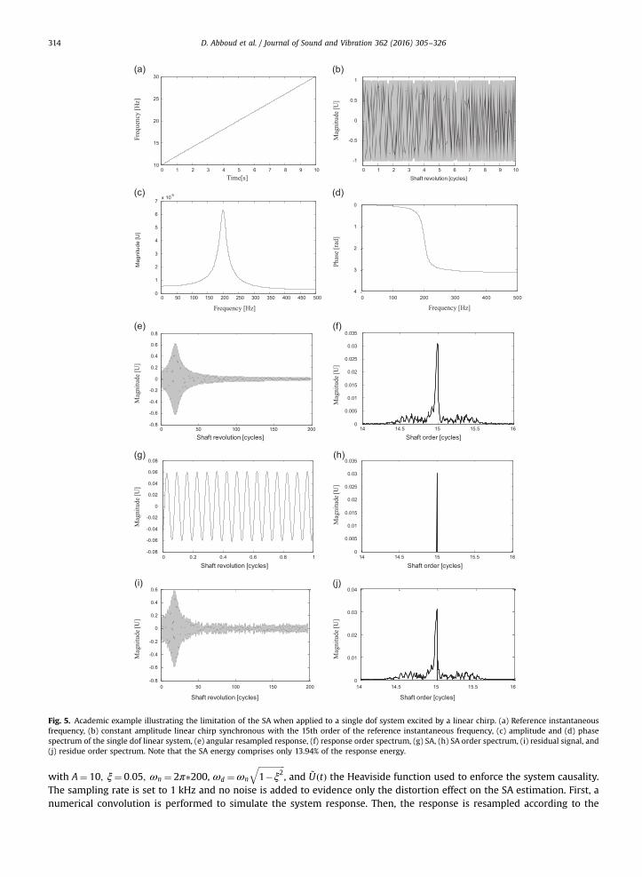
A natural way to model the effect of the transmission path in rotating machines is by exciting a single degree-of-freedom(dof) system by a constant-amplitude chirp. Though being physically simplistic,2 the chirp is chosen with constant ampli-tude to clearly reveal the amplitude distortion. Fig. 5(a) illustrates the time evolution of the reference instantaneous fre-quency f i tð Þ ¼ 2tþ10, (b) represents the excitation chirp synchronous with the 15th order i.e. ~X tð Þ ¼ sin 2π U15

R t0 f i sð Þds

� ,

and (c) and (d) represents the amplitude and the phase spectrum of the simulated system, respectively, with impulseresponse

~h tð Þ ¼ Aωd

e� jξωnt sin ωdtð Þ ~U tð Þ; (22)

2 In general, the excitation is subjected to an energy modulation owing to changes of the machine power intake as the speed varies. Yet, these changescan still be generally modeled as a speed dependent amplitude distortion in the response.

0 1 2 3 4 5 6 7 8 9 1010

15

20

25

30

0 50 100 150 200-0.8

-0.6

-0.4

-0.2

0

0.2

0.4

0.6

0.8

Shaft revolution [cycles]

0 0.2 0.4 0.6 0.8 1-0.08

-0.06

-0.04

-0.02

0

0.02

0.04

0.06

0.08


0 50 100 150 200-0.8

-0.6

-0.4

-0.2

0

0.2

0.4

0.6


0 1 2 3 4 5 6 7 8 9 10

-1

-0.5

0

0.5

1


0 100 200 300 400 500-4

-3

-2

-1

0

14 14.5 15 15.5 160

0.005

0.01

0.015

0.02

0.025

0.03

0.035

Shaft order [cycles]

14 14.5 15 15.5 160

0.01

0.02

0.03

0.04


14 14.5 15 15.5 160

0.005

0.01

0.015

0.02

0.025

0.03

0.035


Frequency [Hz]

Mag

nitu

de [U

]

Time[s]

Frequency [Hz]

Mag

nitu

de [U

]M

agni

tude

[U]

Mag

nitu

de [U

]M

agni

tude

[U]

Mag

nitu

de [U

]

Phas

e [r

ad]

Mag

nitu

de [U

]

0 50 100 150 200 250 300 350 400 450 5000

1

2

3

4

5

6

7

Mag

nitu

de [U

]

x 10

Freq

uenc

y [H

z]

Fig. 5. Academic example illustrating the limitation of the SA when applied to a single dof system excited by a linear chirp. (a) Reference instantaneousfrequency, (b) constant amplitude linear chirp synchronous with the 15th order of the reference instantaneous frequency, (c) amplitude and (d) phasespectrum of the single dof linear system, (e) angular resampled response, (f) response order spectrum, (g) SA, (h) SA order spectrum, (i) residual signal, and(j) residue order spectrum. Note that the SA energy comprises only 13.94% of the response energy.


with A¼ 10; ξ¼ 0:05; ωn ¼ 2π�200, ωd ¼ωn

ffiffiffiffiffiffiffiffiffiffiffiffiffi1�ξ2

q, and ~U tð Þ the Heaviside function used to enforce the system causality.

The sampling rate is set to 1 kHz and no noise is added to evidence only the distortion effect on the SA estimation. First, anumerical convolution is performed to simulate the system response. Then, the response is resampled according to the


reference instantaneous frequency; this is displayed in Fig. 5(e) with the corresponding order spectrum in (f). Clearly, theamplitude distortion is prominent in the angular domain and manifests itself with long-term energy modulations, whereasthe phase blur is materialized by leakage in the vicinity of the excitation order 15.

It is worth noting that the nature of the deterministic component changes at the system output (see Eq. (9): whereas theexcitation is angle-periodic, the response is not albeit it conserves cyclic rhythms related to the excitation. As a matter offact, these rhythms are captured by the complex exponential kernels in Eq. (9). Last, the SA and the corresponding residueare computed and displayed in Fig. 3(g) and (i), together with their order spectra in Fig. 5(h) and (j), respectively. Noticeably,the SA energy forms only 13.94% of the deterministic signal energy, indicating a poor estimation even in the absence ofrandom noise.

4.2. Evaluation of the GSA

First, it is beneficial to illustrate the GSA on the previous simulated response. For this purpose, the speed varying marginis first divided into 20 non-overlapping regimes of 1 Hz width (i.e. δω¼ 2π rad=s) and the smoothed estimator of the GSA isapplied on the noise-free signal. The smoothed parameter of the interpolation kernel (normal window) is chosen equal tothe speed resolution. Results are displayed in Fig. 6 wherein (a) represents the deterministic component as well as the GSAestimate and (b) illustrates their corresponding order spectra. A significant enhancement over the SA is seen: the GSAestimate has the ability of tracking the temporal variations of the amplitude and of the phase, capturing 92.43% of the actualsignal energy. It is also noticed that the estimator underestimates the actual response in the vicinity of the resonance(around cycle 20,000) as predicted by the statistical analysis of Section 3.3.1.

Second, a white Gaussian noise is added on the response to obtain a SNR¼2 and the signal duration is enlarged 10 times(i.e. one million samples) while keeping the same speed variation. In an attempt to evaluate the influence of the speedresolution, the GSA is estimated for different interval widths (4 Hz, 1.5 Hz, 0.5 Hz and 0.33 Hz). One can notice the poorestimation when performed on 4 Hz width, whereas significant enhancement is perceived as δω decreases. With the aim ofquantifying this dependence, the GSA energy is evaluated with respect to the actual response energy for different speedresolutions, δω¼ Δω

R (where Δω is the speed varying margin) and results are depicted in Fig. 7(b). In accordance to thestatistical results obtained in Section 3.3.1, the estimated energy increases with resolution R (i.e. the interval widthdecreases) so as to finally reach an asymptotic value. Note that the difference between the asymptotic and the ideal value(100%) corresponds to the estimator bias for the selected parameters.

Eventually, it is noteworthy that the speed resolution cannot be taken arbitrary small because the number of averages,card Κr

� �, then decreases to zero. Therefore, a trade-off is to be made between these quantities. Accordingly, it is also

beneficial to evaluate the estimation accuracy with respect to the signal length. To do so, the evolution of the estimated GSAenergy is calculated with respect to the signal length for different speed resolutions, yet conserving the same speed var-iation (see Fig. 8). Interestingly, the obtained curves consist of a transient and a steady state: whereas the former reflects thestochastic variability of the estimator, the latter is representative of the bias. This illustrates the bias-variance trade-off.

0 0.2 0.4 0.6 0.8 1 1.2 1.4 1.6 1.8 2-1

-0.5

0

0.5

1Actual deterministic responseEstimated response (GSA)

14 14.2 14.4 14.6 14.8 15 15.2 15.4 15.6 15.8 160

0.01

0.02

0.03

0.04Actual deterministic responseEstimated response (GSA)

underestimation

Mag

nitu

de [

]M

agni

tude

[] X

Fig. 6. (a) Actual deterministic response and GSA estimate together with their (b) order spectra. The estimation comprises 92.43% of the energy of theactual response.

14.96 14.97 14.98 14.99 15 15.01 15.02 15.03 15.040

0.005

0.01

0.015

0.02

0.025

0.03

0.035

Mag

nitu

de [

]

0 10 20 30 40 50 600

102030405060708090

100

ener

gy [%

]

Regime number

Actual responseGSA estimation =2 *4 rad/sGSA estimation =2 *1.25 rad/sGSA estimation =2 *0.5 rad/sGSA estimation =2 *0.33 rad/s

δΩδΩ

δΩδΩ

πππ

π

Fig. 7. (a) Order spectrum of the actual response and GSA estimates obtained with different speed resolutions and (b) percentage evolution of the GSAenergy (with respect to the energy of the actual response) with the numbers of regimes for 10 s time record.

0 50 100 150 200 250 300 350 400 450 50030

40

50

60

70

80

90

100

110

120

130

Bias

Per

cent

age

of e

stim

atio

n en

ergy

[%]

Time records [s]

Fig. 8. Percentage evolution of the GSA energy (with respect to the energy of the actual response) with the number of regimes for 10 s time record.


5. Experimental validation

Similarly to the SA, the field of applications of the GSA covers multiple mechanical applications such as: machinediagnostics, separation of mechanical sources and identification of mechanical system [1]. This section reports a typicalexample in the field of rotating machine diagnostic, where deterministic gear related components contribute to the SES andmask the bearing fault signature—originally random. The aim is to show how to take advantage of the GSA to enhance theenvelope-based diagnosis of rolling element bearings when operating under nonstationary condition. After a briefdescription of the test rig and experimental protocol, the concept of the GSA is demonstrated on gear vibration signals. Then,the GSA is used to extract the gear signal from its noisy environment. Last, the benefit of the separation is illustrated byanalyzing the envelope of the residual signal in order to diagnose the bearings.

5.1. Test rig and experimental protocol

The test rig used in this paper is located at Cetim3 and illustrated in Fig. 9. It essentially comprises an asynchronousmotor supplied by a variable-speed drive to control the motor speed, followed by a spur gear with 18 teeth and ratio of 1.The gear is subjected to excessive wear. Two identical rolling element bearings are installed behind the spur gear; thehealthy one (denoted as B1) is closer to the gears than the faulty one (denoted as B2) which is coupled to an alternator bymeans of a belt to impose a constant load. Bearing characteristics are listed in Table 1. An optical keyphasor of type “Brawn”is fixed close to the motor output to measure the rotational shaft position. In addition, two accelerometers, hereafterdenoted as “Acc1” and “Acc2”, are respectively branched on bearings B1 and B2 in the Z-direction to measure the producedvibrations. The sampling rate is set to 25.6 kHz.

First, experimental tests are conducted wherein five different constant speeds are imposed by the speed drive during 10 sin order to obtain five records for each accelerometer. Fig. 10 illustrates the raw signals measured by accelerometers Acc1and Acc2 at the chosen speeds 650, 950, 1250, 1550 and 1850 rev/min. The importance of such an experiment is to obtain an

3 Technical Center for Mechanical Industries—Senlis, France.

Acc1Parallel gear(ratio 1)

Keyphasor

Bearing 1(Healthy)

Bearing 2(Faulty)

Motor Acc2

Reference shaft

Fig. 9. The test rig located at CETIM.

Table 1Characteristic of the rolling element bearing (Deep groove ball 6820).

Pitch diameter[mm]

Rolling elementdiameter [mm]

Number of roll-ing elements

Contactangle

Outer, housing,diameter [mm]

Inner, bore, dia-meter [mm]

Ball pass order-outer race(BPOO)

Ball pass order-inner race(BPOI)

25 6 8 0.00 35 15 3.04 4.96


actual reference of the machine behavior at the chosen operating speeds (which explains why they have been uniformlyseparated to systematically cover the machine operating margin). In the second experiment, a runup (from 500 to 2000 rev/min) and a random speed profile (between 500 and 2500 rev/min) are imposed to the electric motor over 52 s; the acquiredacceleration signals are illustrated in Fig. 11 together with their corresponding speed profiles. Whereas the former type ofspeed profile is frequently met in rotor dynamics, the latter is for instance encountered in wind turbine applications.

5.2. Validation of the GSA

5.2.1. Evaluation of GSA under different speed profilesBy construction, the GSA theoretically returns the SA of a vibration signal at any operating speed independently of the

speed profile in the record. The principal object of this section is to experimentally evidence this statement. For this purpose,the GSA is applied on variable speed records at some speeds, while the SA is applied on the constant-speed records at the samespeeds. Since comparisons should be performed on estimations, the corresponding estimator errors (i.e. bias and variance)should be considered. Thus, the bias and the variance of the GSA should be theoretically calculated by means of theequations developed in Section 3.3, and used to build a threshold. The idea is to evaluate whether the difference betweenthe GSA- and SA-based estimate are below the estimation threshold. If so, the aforementioned statement will be experi-mentally demonstrated.

To do so, the SA is applied to both acceleration signals on the constant-speed records of the first experiment (which isnothing else then the GSA applied to stepwise speed profile) in order to obtain a reference against which the GSA can becompared. Since the gears have a unit ratio, the reference period used in the average is set equal to the gear rotation, whichmakes possible to account for gear modulations. Next, the GSA is performed on the same accelerometer signal (Acc1) as inthe case of (i) runup and (ii) random speed varying profiles. In order to evaluate the statistical performance of the estimator,it is proposed to compute the average values of the absolute bias and of the variance with respect to the SA.4 The averageabsolute bias at the operating speed ωr is estimated by averaging the absolute value returned by Eq. (19) over the cycleduration, i.e.

bb ωrð Þ ¼ 1Θ

Z Θ

0Bias bmY θ;ωr

� n o dθ; (23)

whereas the average variance is estimated by averaging the value returned by Eq. (20) over the cycle duration, i.e.

bσ2 ωrð Þ ¼ 1Θ

Z Θ

0Var bmY θ;ωr

� n o dθ; (24)

4 The distributions mY ̅θ ;ωr� �

and PY ̅θ ;ωr� �

are returned by the SAs of the signals and of the residual powers, respectively, applied on the constant-speed records of the first experiment.

0 1 2 3 4 5 6 7 8 9 10-100

-50

0

50

100Acc1Acc2

0 1 2 3 4 5 6 7 8 9 10-100

-50

0

50

100Acc1Acc2

0 1 2 3 4 5 6 7 8 9 10100

-50

0

50

100Acc1Acc2

0 1 2 3 4 5 6 7 8 9 10-100

-50

0

50

100Acc1Acc2

0 1 2 3 4 5 6 7 8 9 10-100

-50

0

50

100Acc1Acc2

Time [s]

Time [s]

Time [s]

Time [s]

Time [s]

Fig. 10. (a) Acceleration signals acquired at operating speeds (a) 650 rev/min, (b) 950 rev/min, (c) 1250 rev/min, (d) 1550 rev/min and (e) 1850 rev/min.


Having an estimate of the average bias and variance, the level of the estimation error can be evaluated as

thres¼ bb ωrð Þþ3Ubσ ωrð Þ: (25)

In the runup case, the comparisons between the GSA estimates and the SA-based references are displayed in Fig. 12 forthe shaft speeds (a) 650, (b) 950, (c) 1250, (d) 1550 and (e) 1850 rev/min (the speeds under which the first experiment hasbeen conducted); the absolute value of the corresponding estimation errors are illustrated in (f)–(j) together with thecalculated thresholds. Results for the case of varying speed profile are reported in Fig. 13. In general, the similarity betweenthe estimated signatures is remarkable for both cases: the estimation error mostly stays below the threshold at theexception of some phase mismatch at 1250 rev/min (see the third raw in Figs. 12 and 13). This confirms the model given inEq. (9). Also, since the estimation performance does not show dependence on the speed profile (runup or random variablespeed), one can claim that signal statistics do not depend on higher derivatives of θ, which validates the assumption leadingto Eq. (7). It is worth noting that, despite being below the threshold, the estimation errors of the regimes 650 rev/min (seeFigs. 12(f) and 13(f)) and 1850 rev/min (see Figs. 12(j) and 13(j)) are high. According to Eq. (20), the high error in the formeris due to the low number of cycles associated with the regime, while the high error in the second is due to the high meaninstantaneous power.

Next, the GSA applied on runup and random speed profiles are compared in Fig. 14. The similarity of the compared plotsindicates the invariance of the process properties (i.e. the CNS field) whatever the speed trajectory. Last, the GSA is applied

Fig. 11. (a) Runup speed profile and (b) its corresponding acceleration signals (Acc1 and Acc2). (c) Random speed profile and (d) its correspondingacceleration signals (Acc1 and Acc2).

0 0.2 0.4 0.6 0.8 1-1

0

1

SA-based referenceGSA

0 0.2 0.4 0.6 0.8 1-2

0

2

0 0.2 0.4 0.6 0.8 1-2

0

2

0 0.2 0.4 0.6 0.8 1-5

0

5

0 0.2 0.4 0.6 0.8 1-5

0

5

0 0.2 0.4 0.6 0.8 10

0.5

1Bias=0.092076 ; Std=0.089369

Estimation differenceBias+3.Std

0 0.2 0.4 0.6 0.8 10

1

2Bias=0.032804 ; Std=0.10853

0 0.2 0.4 0.6 0.8 10

2

4Bias=0.067231 ; Std=0.14055

0 0.2 0.4 0.6 0.8 10

2

4Bias=0.014904 ; Std=0.16227

0 0.2 0.4 0.6 0.8 10

1

2Bias=0.13501 ; Std=0.19656

Shaft revolution [rev]Shaft revolution [rev]

Mag

nitu

de [

]

Mag

nitu

de [

]

Fig. 12. Comparison between the SA of Acc1 signal acquired at constant speeds and the GSA of the same accelerometer acquired in runup: (a) 650 rev/min,(b) 950 rev/min, (c) 1250 rev/min, (d) 1550 rev/min, (e) 1850 rev/min; (f)–(j) are the absolute differences of the plots in (a)–(e) respectively and theircorresponding threshold.


on signal Acc1 of the runup speed profile (Fig. 11(b)) together with the classical SA. Results are displayed in Fig. 15 whereinthe same unit scale is used to evidence the amplitude differences. As expected from the theory, the deterministic com-ponent varies with speed in terms of phase and energy (see Fig. 15(b–f)) which results in an attenuation of the SA magnitude(see Fig. 15(a)).

5.2.2. Extraction of the gear contributionIn the following, the efficiency of the GSA in extracting the deterministic component is investigated. For this purpose, the

GSA is applied on vibration signals produced under runup and random regimes in order to extract the deterministic gearrelated components under both cases. The GSA estimates of signals Acc1 and Acc2 in runup computed with 20 non-overlapped intervals are displayed in Fig. 16(a) and (d) runup and the corresponding amplitude order spectra are displayed

0 0.2 0.4 0.6 0.8 1-1

0

1SA-based referenceGSA

0 0.2 0.4 0.6 0.8 1-2

0

2

0 0.2 0.4 0.6 0.8 1-2

0

2

0 0.2 0.4 0.6 0.8 1-5

0

5

0 0.2 0.4 0.6 0.8 1-5

0

5

0 0.2 0.4 0.6 0.8 10

0.5

1Bias=0.092076 ; Std=0.089369 Estimation difference

Bias+3.Std

0 0.2 0.4 0.6 0.8 10

1

2Bias=0.032804 ; Std=0.10853

0 0.2 0.4 0.6 0.8 10

2

4

Bias=0.067231 ; Std=0.14055

0 0.2 0.4 0.6 0.8 10

2

4Bias=0.014904 ; Std=0.16227

0 0.2 0.4 0.6 0.8 10

1

2Bias=0.13501 ; Std=0.19656

Shaft revolution [rev]Shaft revolution [rev]

Mag

nitu

de [

]

Mag

nitu

de [

]

Fig. 13. Comparison between the SA of signal Acc1 acquired at constant speeds and the GSA of the same accelerometer acquired in random variable speed:(a) 650 rev/min, (b) 950 rev/min, (c) 1250 rev/min, (d) 1550 rev/min, (e) 1850 rev/min; (f)–(j) are the absolute differences of the plots in (a)–(e) respectivelyand their corresponding threshold.

Fig. 14. Comparison between the GSA of signal Acc1 acquired at runup and the GSA of the same accelerometer acquired at random variable speed:(a) 650 rev/min, (b) 950 rev/min, (c) 1250 rev/min, (d) 1550 rev/min, (e) 1850 rev/min; (f)–(j) are the close-ups between 0 and 0.3 rev of plots (a)–(e) respectively.


Fig. 15. Classical SA (a) and GSA applied on signal Acc1 in runup speed profile for the speeds (b) 650 rev/min (c), 950 rev/min (d), 1250 rev/min (e),1550 rev/min and (f) 1850 rev/min. The same unit scale is used to evidence the differences.

1 meshing order

2 meshing order

3 meshing order4 meshing order

1 meshing order

2 meshing order

3 meshing order 4 meshing order

Energy leakageEnergy leakage

0 100 200 300 400 500 600 700 800 900 1000 0 100 200 300 400 500 600 700 800 900 1000

0 10 20 30 40 50 60 70 80 90 100 0 10 20 30 40 50 60 70 80 90 100

17 17.2 17.4 17.6 17.8 18 18.2 18.4 18.6 18.8 19 17 17.2 17.4 17.6 17.8 18 18.2 18.4 18.6 18.8 19

20

15

10

5

0

-5

-10

-15

-20

0

5

10

15

-15

-10

-5

0.05

0.1

0.15

0.2

0.25

0.3

0.35

0 0

0.02

0.04

0.06

0.08

0.1

0.12

0.14

0.16

0.05

0.1

0.15

0.2

0.25

0.05

0.15

0.1

Fig. 16. (a) GSA of signal Acc1 in runup speed regime estimated with 20 non-overlapping intervals, (b) its amplitude order spectrum and (c) its zoomaround the 1st meshing order. (d) GSA estimate of signal Acc2 in random speed regime estimated with 20 non-overlapping intervals, (e) its amplitudeorder spectrum and (f) its zoom around the 1st meshing order.



in (b) and (e), respectively. Observing its evolution in the angular domain (see Fig. 16(a) and (d)), the GSA is able to track theenergy variations of the deterministic component.

Observing its order-domain counterpart (see Fig. 16(a) and (d)), the GSA seems to have a similar behavior of the SA: itpresents equally spaced harmonics as if a comb filter was applied. Yet, when checking these harmonics (see Fig. 16(c) and(f)), one can clearly notice the energy leakage around the considered orders. This actually means that—in some sense—theGSA has tracked the (amplitude and phase) distortions due to the TF of the system. It is worth noting that the energy leakagearound the harmonics is dependent on the speed variability in the record. The higher this variability is, the higher theinduced leakage. This can be simply checked by comparing the broadening of the harmonics in Fig. 16(c) and (f). The widthof the harmonics is wider for the random regime than for the runup because speed variability is greater in the former case.

In order to consolidate the GSA results, the next step is to investigate the residual signal obtained from subtracting theGSA estimate from the original signal. In the case of a perfect estimation, the broadened harmonics related to the deter-ministic component should be absent from the residues. For this purpose, the amplitude order spectrum of the SA and GSAresidues signals are compared in Fig. 17 for Acc2 signal in runup regime and Acc1 signal in random speed-varying regime. Asexpected, the SA fails in both cases to eliminate the deterministic component wherein a significant part of the harmonic stillexists. In details, the SA is equivalent to applying a narrow-band comb filter spaced with the machine order, thus it is unableto entirely extract the broadened harmonics as they fall outside the lobes of the comb filter. Therefore, once can see a localfall at all the meshing order harmonics in all the plots of Fig. 17. Interestingly, the GSA evidences almost total suppression,thus validating its efficiency in extracting the deterministic component in variable speed conditions.

17.94 17.96 17.98 18 18.02 18.04 18.06

0.05

0.1

0.15

0.2

0.25

0.3

shaft order [evt/rev]

mag

nitu

de [m

/s-2]

Raw signalSA residualGSA residual

35.95 36 36.050

0.05

0.1

0.15

0.2

0.25


mag

nitu

de [m

/s-2]


17.94 17.96 17.98 18 18.02 18.04 18.060

0.05

0.1

0.15

0.2


mag

nitu

de [m

/s-2]


35.95 36 36.050

0.02

0.04

0.06

0.08

0.1


mag

nitu

de [m

/s-2]


53.95 54 54.050

0.01

0.02

0.03

0.04

0.05


mag

nitu

de [m

/s-2]


53.95 54 54.050

0.01

0.02

0.03

0.04

0.05


mag

nitu

de [m

/s-2]


Local fall caused by the SA








Fig. 17. Amplitude order spectrum of the SA and GSA residues of Acc2 in runup speed regime, close-ups around (a) the 1st meshing harmonic, (b) the 2ndmeshing harmonic and (c) the 3rd meshing harmonic. Amplitude order spectrum of the SA and GSA residues of Acc1 signal in random speed-varyingregime, close-ups around (d) the 1st meshing harmonic, (e) the 2nd meshing harmonic and (f) the 3rd meshing harmonic.


5.3. Envelope enhancement

In vibration analysis of rotating machine, the squared envelope spectrum (SES) is one of the most efficient indicators forthe assessment of CS2 sources which are typical symptoms of damage in rolling element bearing faults [35]. Similarly toother CS2 tools, the SES should be applied on the pure random part of the signal; otherwise spurious harmonics may appearand hide the actual second-order content. In speed varying regimes, the SES is combined with computed order tracking toobtain an order-domain representation. This section reports a typical issue in the field of rotating machine diagnostic, wheredeterministic gear related components contribute to the SES and mask the bearing fault signature—originally random. Theprincipal object is to investigate the benefits brought by the GSA in enhancing the envelope analysis for bearing faultdetection.

For this purpose, Acc2 signal in runup speed regime is picked up to evaluate the signature of the faulty bearing. Next,after angular resampling, the SES is applied on the raw signal over the entire order band, on the SA residue and on the GSAresidue as shown in the diagram of Fig. 18. The obtained results are reported in Fig. 19. As expected, the SES of the raw signalevidences several misleading harmonics synchronous with the reference shaft order, whereas slight enhancement is per-ceived after removing the SA (see Fig. 19(a) and (b)). Noticeably, the SES of the residual signal after removing the GSA muchbetter evidences the bearing signature (see Fig. 19(c)), thus demonstrating the utility of the introduced technique forenvelope based vibration analysis.

6. Conclusion

The object of this paper was to extent the synchronous average, traditionally applied to cyclostationary signals, to thegeneral class of cyclo-non-stationary (CNS) signals wherein the operating speed is allowed to be nonstationary. It has beenshown that, in the case of a system operating under variable speed, cyclo-non-stationarity can be produced by the transferfunction from the excitation to the accelerometer. This phenomenon induces systematic changes in the signal phase andmagnitude, thus changing its structure. These changes have been modeled by means of an explicit dependence on thespeed. As a consequence, the deterministic part loses its (angle-) periodicity, thus jeopardizing the synchronous average.

Therefore, a novel quantity coined the “generalized synchronous average (GSA)” has been introduced to extract thedeterministic part of a CNS signal. This quantity, when evaluated at an arbitrary speed, has the advantage of expressing themean value of the signal as if the system was operating steadily at that speed. Two estimators of the GSA have beenproposed. The first one returns the synchronous average of the signal at predefined discrete operating speeds. A briefstatistical study of it is performed, aiming to provide the user with confidence intervals that reflect the “quality” of theestimator according to the SNR and the estimated speed. The second estimator returns a smoothed version of the former byenforcing continuity over the speed axis. It helps to reconstruct the deterministic component by tracking a specific tra-jectory dictated by the speed profile (assumed to be known a priori). The proposed approach has been tested on an actualbenchmark comprising a typical powertrain. The aim was twofold: first to validate the proposed CNS model and the GSAestimators and second to show the usefulness of the proposed approach for rolling element bearing diagnostics in variableoperating speed. Interestingly, the GSA proved efficient in estimating the deterministic gear contribution, showing con-siderable enhancement over the classical SA.

Fig. 18. Comparison of the SES of residue, the SES of SA residue and the SES of the GSA residue.

Fig. 19. SES of the (a) resampled signal, (b) the SA residue and (c) the GSA residue applied on signal Acc2 in runup.


Limitations of the GSA are inherently related to estimation issues. In particular, it has been assumed that the speedvariations are slower than the signal cycle; although this condition seems reasonable in several applications, it can easily berelaxed in the general case by averaging portions of signal smaller than cycles. Another issue concerns the setting of theestimation parameters such as the speed resolution, the number of regimes, and the repartition of the central frequencies. Inthe present paper, these settings have been governed by simplicity. For example, the regimes were chosen to be uniformlydistributed along the speed axis. This actually makes the estimation variance dependent on the operating speed; again, thiscould easily be alleviated by allowing the speed resolution to be inversely proportional to the speed probability distribution.

Eventually, authors believe that the GSA can be also used for estimating second-order quantities such as instantaneousautocorrelation or the spectral correlation as functions of speed. As well, it can be applied to other domains such as geardiagnostics, noise separation in IC engines, etc.

Acknowledgments

This work was conducted in the framework of the LabEx CeLyA ("Centre Lyonnais d'Acoustique", ANR-10-LABX-60).

Appendix

a) Proof of Eq. (19).

Let us now apply the statistical expectation to the raw estimator of the GSA applied to the model in Eq. (8)

E bmY θ;ωr

� n o¼ E

1card Κr

� �XkAΚr

Xα

cαY θþkΘ;ω θþkΘ� �

ej2παθþ kΘð ÞΘ �

" ):

((A1)

By exploiting the linearity of the expectation operator

E bmY θ;ωr

� n o¼ 1card Κr

� �XkAΚr

Xα

cαY ω θþkΘ� �

ej2παθþ kΘð ÞΘ

#:

"(A2)


According to Slutsky’s theorem on probability limits, the sample averaging operator 1card Κrf g

PkAΚr

�f g converges to the

statistical expectation Eω �f g with respect to the distribution of ω θþkΘ�

in the interval ωr� δω2 ;ωr� δω

2

� �; i.e.

E bmY θ;ωr

� n o¼ Eω

Xα

cαY ωð Þej2παθΘg ¼ Eω mY θ;ω

� n o:

((A3)

The rest of the proof follows by approximating the distribution of ω by a uniform law in the intervalωr�δω=2;ωrþδω=2� �

and after performing a second-order Taylor approximation around ωr .a) Proof of Eq. (20).

Similarly to the previous proof, the variance is

Var bmY θ;ωr

� n o¼ Var

1card Κr

� �XkAΚr

Xα

cαY θþkΘ;ω θþkΘ� �

ej2παθþ kΘð ÞΘ

��:

"((A4)

Since terms in the sum do not overlap

Var bmY θ;ωr

� n o¼ 1

card Κr� �� 2XkAΚr

PY θþkΘ�

;ω θþkΘ� �

(A5)

where PY θ;ω�

¼ VarPαcαY θ;ω�

ej2παθΘ

��is the instantaneous power of the residue (i.e. purely random) that depends on

the speed. According to Slutsky’s theorem

Var bmY θ;ωr

� n o¼ 1card Κr

� �Eω PY θ;ω� n o

(A6)

The rest of the proof follows by approximating the distribution of ω by a uniform law and performing a second-orderTaylor approximation around ωr .

References

[1] J. Antoni, Cyclostationary by examples, Mechanical Systems and Signal Processing 23 (4) (2009) 987–1036.[2] J. Antoni, R.B. Randall, Differential diagnosis of gear and bearing faults, Journal of Sound and Vibration 124 (2) (2002) 165–171.[3] J. Antoni, R.B. Randall, Unsupervised noise cancellation for vibration signals: Part II—a novel frequency-domain algorithm, Mechanical Systems and

Signal Processing 18 (2004) 103–117.[4] R.B. Randall, Vibration-Based Condition Monitoring: Industrial, Automotive and Aerospace Applications, John Wiley and Sons, West Sussex, 2011.[5] S. Braun, The extraction of periodic waveforms by time domain averaging, Acustica 32 (1975) 69–77.[6] P.D. McFadden, M. Toozhy, Application of synchronous averaging to vibration monitoring of rolling element bearing, Mechanical Systems and Signal

Processing 14 (2000) 891–896.[7] K.R. Fyfe, E.D.S. Munck, Analysis of computed order tracking, Mechanical Systems and Signal Processing 11 (2) (1997) 187–205.[8] P.D. McFadden, Interpolation techniques for time domain averaging of gear vibration, Mechanical Systems and Signal Processing 3 (1) (1989) 87–97.[9] F. Bonnardot, M. ElBadaoui, R.B. Randall, J. Daniere, F. Guillet, Use of the acceleration signal of a gearbox in order to perform angular resampling (with

limited speed fluctuation), Mechanical Systems and Signal Processing 19 (2005) 766–785.[10] J. Antoni, F. Bonnardot, A. Raad, M. El Badaoui, Cyclostationary modelling of rotating machine vibration signals, Mechanical Systems and Signal Pro-

cessing 18 (2004) 1285–1314.[11] C.J. Stander, P.S. Heyns, Transmission path phase compensation for gear monitoring under fluctuating load conditions, Mechanical Systems and Signal

Processing 20 (7) (2006) 1511–1522.[12] P. Borghesani, P. Pennacchi, R.B. Randall, R. Ricci, Order tracking for discrete-random separation in variable speed conditions, Mechanical Systems and

Signal Processing 30 (2012) 1–22.[13] J. Antoni, N. Ducleaux, G. NGhiem, S. Wang, Separation of combustion noise in IC engines under cyclo-non-stationary regime, Mechanical Systems and

Signal Processing 38 (1) (2009) 223–236.[14] M.D. Coats, N. Sawalhi, R.B. Randall, Extraction of tacho information from a vibration signal for improved synchronous averaging, Proceedings of

Acoustics (2009).[15] Z. Daher, E. Sekko, J. Antoni, C. Capdessus, L. Allam, Estimation of the synchronous average under varying rotating speed condition for vibration

monitoring, Proceedings of ISMA (2010).[16] J. Urbanek, T. Barszcz, J. Antoni, A two-step procedure for estimation of instantaneous rotational speed with large fluctuations, Mechanical Systems and

Signal Processing 38 (1) (2013) 96–102.[17] D.A. Wallace, M.S. Darlow, Hilbert transform techniques for measurement of transient gear speeds, Mechanical Systems and Signal Processing 2 (2)

(1988) 187–194.[18] F. Combet, L. Gelman, An automated methodology for performing time synchronous averaging of a gearbox signal without speed sensor, Mechanical

Systems and Signal Processing 21 (6) (2007) 2590–2606.[19] F. Combet, R. Zimroz, A new method for the estimation of the instantaneous speed relative fluctuation in a vibration signal based on the short time

scale transform, Mechanical Systems and Signal Processing 23 (4) (2009) 1382–1397.[20] J. Klapper, J.T. Frankle, Phase-Locked and Frequency-Feedback Systems, Academic Press, New York, 1972.[21] Z. Bin, Z. Dong-lai, Research on synchronous sampling clock jitter of power system, Proceedings of the 2nd International Conference on Information

Engineering and Computer Science (ICIECS), 25 Dec–26 Dec 2010, Wuhan, China.[22] R. Potter, M. Gribler, GRIBLER, Computed order tracking obsoletes older methods, Proceedings of the SAE Noise and Vibration Conference, 1989, pp. 63–

67.[23] W. Potter, Tracking and resampling method and apparatus for monitoring the performanceof rotating machines, United States Patent 4,912,661, 1990.[24] R. Potter, A new order tracking method for rotating machinery, Sound and Vibration 24 (1990) 30–34.

http://refhub.elsevier.com/S0022-460X(15)00750-6/sbref1




















































[25] D. Rémond, J. Antoni, R.B. Randall, Editorial for the special issue on Instantaneous Angular Speed (IAS) processing and angular applications, MechanicalSystems and Signal Processing 44 (1–2) (2014) 1–4.

[26] S. Braun, The synchronous (time domain) average revisited, Mechanical Systems and Signal Processing 25 (4) (2011) 1087–1102.[27] S. Braun, Mechanical Signature Analysis, Academic Press, 1986.[28] D. Abboud, S. Baudin, J. Antoni, D. Remond, M. Eltabach, O. Sauvage, The spectral correlation analysis of cyclo-non-stationary signals, Mechanical

Systems and Signal Processing (2015).[29] M. Rosenblatt, Remarks on some nonparametric estimates of a density function, Annals of Mathematical Statistics 27 (3) (1956) 832.[30] E. Parzen, On estimation of a probability density function and mode, Annals of Mathematical Statistics 33 (3) (1962) 1065.[31] Birge, L., Rozenholc, Y. How many bins should be put in a regular histogram, Prepublication no 721, Laboratoire de Probabilites et Modeles Aleatoires,

CNRS-UMR 7599, Universite Paris VI & VII, 2002.[32] P. Hall, E. Hannan, On stochastic complexity and nonparametric density estimation, Biometrika 75 (4) (1988) 705–714.[33] H. André, F. Girardin, A. Bourdon, J. Antoni, D. Rémond, Precision of the IAS monitoring system based on the elapsed time method in the spectral

domain, Mechanical Systems and Signal Processing 44 (1–2) (2014) 14–30.[34] Q. Leclère, L. Pruvost, E. Parizet, Angular and temporal determinism of rotating machine signals: the diesel engine case, Mechanical Systems and Signal

Processing 24 (7) (2010) 2012–2020.[35] R.B. Randall, J. Antoni, Rolling element bearing diagnostics—a tutorial, Mechanical Systems and Signal Processing 25 (2) (2011) 485–520.





















Deterministic-random separation in nonstationary regime

Documents

Transcript of Deterministic-random separation in nonstationary regime