application to nonstationary circadian rhythms
50
This is a repository copy of Wavelet spectral testing : application to nonstationary circadian rhythms. White Rose Research Online URL for this paper: https://eprints.whiterose.ac.uk/142815/ Version: Accepted Version Article: Hargreaves, Jessica Kate orcid.org/0000-0002-7173-7902, Knight, Marina Iuliana orcid.org/0000-0001-9926-6092, Pitchford, Jonathan William orcid.org/0000-0002-8756- 0902 et al. (4 more authors) (2019) Wavelet spectral testing : application to nonstationary circadian rhythms. Annals of Applied Statistics. pp. 1817-1846. ISSN 1932-6157 https://doi.org/10.1214/19-AOAS1246 [email protected] https://eprints.whiterose.ac.uk/ Reuse Items deposited in White Rose Research Online are protected by copyright, with all rights reserved unless indicated otherwise. They may be downloaded and/or printed for private study, or other acts as permitted by national copyright laws. The publisher or other rights holders may allow further reproduction and re-use of the full text version. This is indicated by the licence information on the White Rose Research Online record for the item. Takedown If you consider content in White Rose Research Online to be in breach of UK law, please notify us by emailing [email protected] including the URL of the record and the reason for the withdrawal request.
-
Upload
khangminh22 -
Category
Documents
-
view
0 -
download
0
Transcript of application to nonstationary circadian rhythms

This is a repository copy of Wavelet spectral testing : application to nonstationary circadian rhythms.
White Rose Research Online URL for this paper:https://eprints.whiterose.ac.uk/142815/
Version: Accepted Version
Article:
Hargreaves, Jessica Kate orcid.org/0000-0002-7173-7902, Knight, Marina Iuliana orcid.org/0000-0001-9926-6092, Pitchford, Jonathan William orcid.org/0000-0002-8756-0902 et al. (4 more authors) (2019) Wavelet spectral testing : application to nonstationary circadian rhythms. Annals of Applied Statistics. pp. 1817-1846. ISSN 1932-6157
https://doi.org/10.1214/19-AOAS1246
[email protected]://eprints.whiterose.ac.uk/
Reuse
Items deposited in White Rose Research Online are protected by copyright, with all rights reserved unless indicated otherwise. They may be downloaded and/or printed for private study, or other acts as permitted by national copyright laws. The publisher or other rights holders may allow further reproduction and re-use of the full text version. This is indicated by the licence information on the White Rose Research Online record for the item.
Takedown
If you consider content in White Rose Research Online to be in breach of UK law, please notify us by emailing [email protected] including the URL of the record and the reason for the withdrawal request.
Submitted to the Annals of Applied Statistics
arXiv: arXiv:0000.0000
WAVELET SPECTRAL TESTING: APPLICATION TO NONSTATIONARY
CIRCADIAN RHYTHMS
BY JESSICA K. HARGREAVES∗ , MARINA I. KNIGHT
∗ , JON W. PITCHFORD† ,
RACHAEL J. OAKENFULL‡ , SANGEETA CHAWLA
‡ , JACK MUNNS‡
AND SETH J.
DAVIS‡
University of York∗, †, ‡
Rhythmic data are ubiquitous in the life sciences. Biologists need re-
liable statistical tests to identify whether a particular experimental treat-
ment has caused a significant change in a rhythmic signal. When these
signals display nonstationary behaviour, as is common in many biologi-
cal systems, the established methodologies may be misleading. Therefore,
there is a real need for new methodology that enables the formal compari-
son of nonstationary processes. As circadian behaviour is best understood
in the spectral domain, here we develop novel hypothesis testing proce-
dures in the (wavelet) spectral domain, embedding replicate information
when available. The data are modelled as realisations of locally station-
ary wavelet processes, allowing us to define and rigorously estimate their
evolutionary wavelet spectra. Motivated by three complementary applica-
tions in circadian biology, our new methodology allows the identification
of three specific types of spectral difference. We demonstrate the advan-
tages of our methodology over alternative approaches, by means of a com-
prehensive simulation study and real data applications, using both pub-
lished and newly generated circadian datasets. In contrast to the current
standard methodologies, our method successfully identifies differences within
the motivating circadian datasets, and facilitates wider ranging analyses of
rhythmic biological data in general.
1. Introduction. Almost all species exhibit changes in their behaviour be-
tween day and night (Bell-Pedersen et al., 2005). These daily rhythms (known
as ‘circadian rhythms’) are the result of an internal timekeeping system, in re-
sponse to daily changes in the physical environment (Vitaterna et al., 2001; Mi-
nors and Waterhouse, 2013). The ‘circadian clock’ enhances survival by directing
anticipatory changes in physiology synchronised with environmental fluctua-
tions. When an organism is deprived of external time cues, its circadian rhythms
typically persist qualitatively but may change in detail; the study of these changes
can reveal the biochemical reactions underpinning the circadian clock and, at a
MSC 2010 subject classifications: Primary 62M10, 60G18; secondary 60-08
Keywords and phrases: wavelets, spectral decomposition, hypothesis testing, circadian
rhythms
Funding: This work was supported by EPSRC. Circadian work in the SJD group is currently
funded by BBSRC awards BB/M000435/1 and BB/N018540/1.
1

2 J. K. HARGREAVES ET AL.
larger scale, can provide valuable insight into the possible consequences of envi-
ronmental and ecological challenges (McClung, 2006; Bujdoso and Davis, 2013).
1.1. Motivation. In many scientific applications, the available data consist
of signals with known group memberships and scientists are interested in estab-
lishing whether these groups display statistically different behaviour. Our work
is motivated by a general problem: biologists need reliable statistical tests to
identify whether a particular experimental treatment has caused a significant
change in the circadian rhythm. If the changes are limited to period and/or
phase then existing Fourier-based theory may be adequate. However, when the
changes to the circadian clock are less straightforward, for example involving
non-stationarity or changes at multiple scales (Hargreaves et al., 2018), the ap-
plication of these established methods may be conducive to misleading conclu-
sions. The value of our approach is illustrated by three complementary exam-
ples, encompassing the effect of various salt stresses on plants, the identifica-
tion of mutations inducing rapid rhythms, and the response of nematode clocks
to pharmacological treatment, as described in the following sections. The bio-
logical experimental details for each dataset appear in Appendix A.
1.1.1. Lead nitrate dataset (Davis Lab, Biology, University of York). This dataset
(henceforth referred to as the ‘Lead dataset’) is from a broad investigation of
whether plant circadian clocks are affected by industrial and agricultural pol-
lutants (Foley et al., 2005; Senesil et al., 1998; Hargreaves et al., 2018; Nicholson
et al., 2003). Specifically, this experiment asks whether lead affects the Arabidop-
sis thaliana circadian clock and, if so, when and how? Figure 1 displays the lu-
minescence profiles for both untreated A. thaliana plants, as well as for those
exposed to lead nitrate.
1.1.2. Ultradian dataset (Millar Lab, Biology, University of Edinburgh). In
order to understand the clock mechanism, a common approach is to mutate
a gene and examine the resulting behaviour in response to a variety of stimuli.
Figure 2 depicts the luminescence profiles recording plant response to light for
both the control and genetically mutated A. thaliana plants (Millar et al., 2015).
Researchers are interested in establishing whether a specific genetic mutation
induced high-frequency behaviour (known as ‘ultradian rhythms’) in the labo-
ratory model plant A. thaliana.
1.1.3. Nematode dataset (Chawla Lab, Biology, University of York). The free-
living nematode Caenorhabditis elegans is an animal widely used in neuroscience
and genetics, but its circadian clock is still poorly understood. To increase un-
derstanding of the nematode clock, and potentially uncover rhythmicity not

WAVELET SPECTRAL TESTING FOR NONSTATIONARY CIRCADIAN RHYTHMS 3
FIG 1. Lead dataset: Luminescence profiles over time for untreated A. thaliana plants (Control)
and those exposed to lead nitrate (Lead). Left: Individuals in the control group (in grey) along with
the group average (blue). Right: Individuals in the lead treatment group (in grey) along with the
treatment group average (red) and the control group average (blue). Each time series has been re-
centred around zero.
detected by conventional approaches, researchers applied a pharmacological
treatment to C. elegans, based on evidence that it causes aberrant circadian rhythms
in other established mammalian and insect circadian models (Kon et al., 2015;
Dusik et al., 2014). Figure 3 depicts the luminescence profiles for both untreated
and treated C. elegans.
On examining Figures 1 and 2, it is visually clear that changes in period and
amplitude between the control and test groups occur in both datasets. Figure 3
reveals apparently similar luminescence profiles for both untreated and treated
C. elegans. Nevertheless, in each experiment, less easily quantified or subtle dif-
ferences between these groups may also exist.
1.2. Aims and structure of the paper. Period estimation is central to the anal-
ysis of circadian data, with the current standard achieving this using Fourier
analysis (Zielinski et al., 2014; Costa et al., 2011) via software packages, such as
BRASS (Biological Rhythm Analysis Software System (Edwards et al., 2010)) or
BioDare (Moore et al., 2014). The practitioner estimates the period of the con-
trol and treatment groups respectively, and then tests for statistically significant
differences (see for example Perea-García et al. (2015), Costa et al. (2011)). Cru-
cially, in all of our motivating examples, such established Fourier-based tests
found no significant difference between groups (see Table S1 in Appendix B.1).
One obvious limitation of this analysis is that the employed methodology

4 J. K. HARGREAVES ET AL.
FIG 2. Ultradian dataset: Luminescence profiles over time for control and mutant A. thaliana
plants. Left: Individuals in the control group (in grey) along with the group average (blue). Right:
Individuals in the mutant group (in grey) along with the mutant group average (red) and the con-
trol group average (blue). Each time series has been re-centred around zero.
FIG 3. Nematode dataset: Luminescence profiles over time for untreated C. elegans (Control) and
those subjected to a pharmacological treatment (Treatment). Left: Individuals in the control group
(in grey) along with the group average (blue). Right: Individuals in the treatment group (in grey)
along with the treatment group average (red) and the control group average (blue). Each time series
has been re-centred around zero.

WAVELET SPECTRAL TESTING FOR NONSTATIONARY CIRCADIAN RHYTHMS 5
does not typically evaluate the crucial underpinning assumption of data station-
arity. In the context examined here, assuming stationarity can be inappropriate
(Hargreaves et al., 2018; Leise et al., 2013), a feature shared by many biological
systems (Zielinski et al., 2014). For our motivating example datasets, we inves-
tigated whether the individual time series are (second-order) stationary via hy-
pothesis testing. We employed two tests for stationarity– a Fourier-based test
(the Priestley-Subba Rao (PSR) (Priestley and Rao, 1969) test) and a wavelet-
based test (Nason, 2013). The results (Table S2 in Appendix B.1) show that, for
each of our motivating example datasets, over 80% of the time series provided
enough evidence to reject the null hypothesis of stationarity. This result suggests
that the application of the current methodology (which assumes data stationar-
ity) would be inappropriate for our motivating datasets and highlights the ur-
gent need for more statistically advanced approaches.
In the specific context of circadian clock data, wavelets have been recognised
as ideally suited to identifying local time and scale features (Leise et al., 2013;
Harang et al., 2012), with time-scale patterns known as indicative of the organ-
ism response to external stimuli (Zielinski et al., 2014). A substantial body of cir-
cadian literature advocates the use of wavelet (Zielinski et al., 2014; Leise et al.,
2013; Harang et al., 2012) and, in particular, spectral representations (Price et al.,
2008) of circadian rhythms. This motivates our choice to formally compare cir-
cadian signals in the wavelet spectral domain by using their time-scale signature
patterns and thus accounting for their proven nonstationary features. Further-
more, we propose to adopt the locally stationary wavelet (LSW) process model of
Nason et al. (2000), which is capable of accounting for data nonstationarity and
crucially has previously demonstrated utility for circadian analysis (Hargreaves
et al., 2018). Modelling nonstationary data within the LSW framework has also
proven successful across a wide variety of fields, from climatology (Fryzlewicz
et al, 2003) and ocean engineering (Killick et al., 2013) to medicine (Nason and
Stevens, 2015) and finance (Fryzlewicz, 2005) corresponding to a multitude of
tasks such as forecasting, change-point detection, spectral estimation and mod-
elling, respectively.
The primary contribution of this work is the development of novel wavelet-
based hypothesis tests that allow for circadian behaviour comparison while ac-
counting for data nonstationarity. This article is organised as follows. Section 2
reviews the theoretical wavelet-based framework we adopt for modelling non-
stationary data and the relevant literature on hypothesis testing in the spectral
domain. Our new hypothesis testing procedures are introduced in Section 3.
Section 4 provides a comprehensive performance assessment of our new meth-
ods via simulation. Section 5 demonstrates the additional insight our techniques
provide for the motivating circadian datasets and Section 6 concludes this work.

6 J. K. HARGREAVES ET AL.
2. Overview: nonstationary processes and hypothesis testing in the spec-
tral domain.
2.1. Modelling nonstationary processes. Many of the statistically rigorous ap-
proaches to modelling nonstationary time series stem from the Cramér-Rao rep-
resentation of stationary processes that states that all zero-mean discrete time
second-order stationary time series {X t }t∈ Z can be represented as
(2.1) X t =
∫π
−πA(ω)exp(iωt )dξ(ω),
where A(ω) is the amplitude of the process and dξ(ω) is an orthonormal in-
crements process (Priestley, 1982). In the representation of stationary processes
above, the amplitude A(ω) does not depend on time, i.e. the frequency behaviour
is the same across time. However, for many real time series, including our circa-
dian datasets, this is unrealistic (Price et al., 2008) and a model where the fre-
quency behaviour can vary with time is needed.
The LSW paradigm provides precisely such a desired setup, and has also proved
to yield superior results when compared to competitor methods in useful tasks
such as classification (e.g. Krzemieniewska et al. (2014) for aerosol spray data)
and clustering (e.g. Hargreaves et al. (2018) for circadian rhythms). Fryzlewicz
(2005) brings strong arguments for the utility of (linear) Gaussian LSW models
for financial data, typically modelled using (non-linear) models, that allow for
time-dependent conditional variance.
In a nutshell, in the LSW framework, the Fourier building blocks in equation
(2.1) are replaced by families of discrete nondecimated wavelets and an LSW
process {X t ;T }T−1t=0 , T = 2J ≥ 1 is represented as follows
(2.2) X t ,T =
J∑
j=1
∑
k∈Z
w j ,k;T ψ j ,k (t )ξ j ,k ,
where {ξ j ,k } is a random orthonormal increment sequence, {ψ j ,k (t ) =ψ j ,k−t } j ,k
is a set of discrete non-decimated wavelets and {w j ,k;T } is a set of amplitudes,
each of which at a scale j and time k. Within each scale j , the amplitudes {w j ,k;T }k
are regulated by a Lipschitz continuous function W j (k/T ), which further fulfils
some technical assumptions in order to allow estimation. Appendix C provides
the background details.
2.1.1. Practical considerations. In this paper, we assume the innovations {ξ j ,k }
to be normally distributed, resulting in modelling the data {X t ,T } as a Gaussian
LSW process. The normality assumption is typically employed for the (Fourier)
circadian testing methodology (Perea-García et al., 2015). This assumption is
WAVELET SPECTRAL TESTING FOR NONSTATIONARY CIRCADIAN RHYTHMS 7
also commonly made in time series analysis in general and in LSW modelling
in particular (e.g. Oh et al. (2003), Van Bellegem and von Sachs (2008) and Na-
son and Stevens (2015)), with Nason (2013) arguing for its non-limiting charac-
ter in this context. In Appendix B.2 we show this assumption is tenable for our
circadian datasets.
The properties of the random increment sequence {ξ j ,k } ensure that {X t ,T } is
a zero-mean process. In practice, for a process with non-zero mean, it is cus-
tomary to re-centre it around zero (Nason, 2010) and this is our approach here,
as the quantity of our primary interest is the process spectral signature.
As is typical for wavelet representations, the data is often required to be of
dyadic length, T = 2J . In many practical applications, this is not realistic and
there are a number of approaches to address this situation (see e.g. Ogden (1997)).
Our approach is to analyse a (dyadic length) segment of the data, with the trun-
cation decided upon careful consultation with the experimental scientists in or-
der to ensure the time-frame of interest is represented.
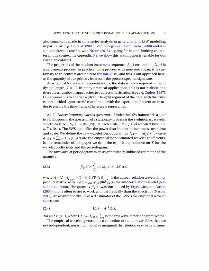
2.1.2. The evolutionary wavelet spectrum. Under the LSW framework, a quan-
tity analogous to the spectrum of a stationary process is the evolutionary wavelet
spectrum (EWS) S j (z) := |W j (z)|2, at each scale j ∈ 1, J and rescaled time z =
k/T ∈ (0,1). The EWS quantifies the power distribution in the process over time
and scale. We define the raw wavelet periodogram as I j ,k;T = |d j ,k;T |2, where
d j ,k;T =∑T
t=0 X t ,T ψ j ,k (t ) are the empirical nondecimated wavelet coefficients.
In the remainder of this paper we drop the explicit dependence on T for the
wavelet coefficients and the periodogram.
The raw wavelet periodogram is an asymptotically unbiased estimator of the
quantity
(2.3) β j (z) =J
∑
i=1
Ai , j Si (z) = (AS) j (z),
where A = (Ai , j )Ji , j=1
= (∑
τΨi (τ)Ψ j (τ))Ji , j=1
is the autocorrelation wavelet inner
product matrix, withΨ j (τ) =∑
k ψ j ,k (0)ψ j ,k (τ) the autocorrelation wavelet (Na-
son et al., 2000). The quantity β j (z) was introduced by Fryzlewicz and Nason
(2006) and is often easier to work with theoretically than the spectrum (Nason,
2013). An asymptotically unbiased estimator of the EWS is the empirical wavelet
spectrum:
(2.4) L(z) := A−1I(z),
for all z ∈ (0,1), where I(z) := (I j ,[zT ])Jj=1
is the raw wavelet periodogram vector.
The empirical wavelet spectrum is a collection of random variables that are
not independent, nor is their (joint or marginal) distribution easy to determine.

8 J. K. HARGREAVES ET AL.
As each coefficient of the empirical wavelet spectrum is a sum of a (typically
logarithmic) number of terms (see equation (2.4)), a mechanism similar to the
central limit theorem brings it closer to normality than the raw wavelet peri-
odogram (Fryzlewicz and Ombao, 2009), which is distributed as a scaled χ21. As
the individual raw periodogram ordinates within each scale are correlated, Fry-
zlewicz and Nason (2006) model the raw wavelet periodogram as approximately
I j ,k ∼β j (z)Z 2j ,k ,
where z = k/T and Z 2j ,k
∼χ21, for j ∈N, k = 0, . . . ,2J −1 = T −1.
A way to ‘correct’ these undesirable features is to employ a transform that
brings the raw periodogram ordinates closer to Gaussianity and decorrelates
within each scale. We adopt the Haar-Fisz transform (denoted F ), introduced
(for spectral estimation) by Fryzlewicz and Nason (2006) and apply it separately
to each scale j = 1, . . . , J of the raw wavelet periodogram, denoted H j ,k;T :=
F I j ,k;T . Proposition 4 in Fryzlewicz and Nason (2006) then suggests a potential
model
H j ,k ∼ N (B j (z),σ2j ),
where B j (z) =Fβ j (z) with z = k/T and F Z 2j ,k
are approximately uncorrelated
N (0,σ2j), again dropping the explicit dependence on T . This model, viewed as
a nonparametric additive regression model, was also employed by Nason and
Stevens (2015) in the context of Bayesian spectral estimation, where its viability
was demonstrated.
2.2. Spectral domain hypothesis testing. Assuming that the available data
consists of multiple nonstationary time series with known group memberships,
to the authors’ knowledge no hypothesis tests exist to determine whether two
groups are significantly different in terms of their associated (evolutionary) wavelet
spectra. Wavelet spectral comparison is closest framed as a (consistent) classifi-
cation method by Fryzlewicz and Ombao (2009), further improved by Krzemie-
niewska et al. (2014). Spectral comparison, framed as testing for spectral con-
stancy, also appears in connection with testing for time series stationarity and
white noise testing. In the Fourier domain, Priestley and Rao (1969) determined
(as a hypothesis test) whether the spectrum is time-varying and, hence, whether
the process is nonstationary. Von Sachs and Neumann (2000) introduced the
principle of assessing the constancy of the time-varying Fourier spectrum by ex-
amining its Haar wavelet coefficients across time. In the wavelet domain, Nason
(2013) developed a test for second-order stationarity which examines the con-
stancy of a wavelet spectrum by also examining its Haar wavelet coefficients. A
similar approach is adopted by Nason and Savchev (2014) in the development
of white noise tests.

WAVELET SPECTRAL TESTING FOR NONSTATIONARY CIRCADIAN RHYTHMS 9
The problem of testing that involves curves is often posed in time series litera-
ture as a functional regression problem defined using a functional response and
categorical predictors (functional ANOVA; see the monograph of Ramsay and
Silverman (2005) for its introduction and the review of Morris (2015) for develop-
ments in the field). Functional regression problems are often treated by projec-
tion in the Fourier or wavelet domain, where the spectral time series representa-
tions become subject to modelling. Shumway (1988) compares groups of curves
(with stationary stochastic errors) by testing whether the mean curves have the
same Fourier spectrum at each given frequency. Fan and Lin (1998) developed
this method by applying the adaptive Neyman test to the (Fourier or wavelet)
transformed difference vector (the difference between the two group-average
time series). Vidakovic (2001) introduces a wavelet-based functional data analy-
sis, with McKay et al. (2012) developing this as an approach for comparing neu-
rophysiological signals that are functions of time. This approach was also sub-
sequently adopted by Atkinson et al. (2017) to develop model validation using a
test statistic based on thresholded wavelet coefficients. Tavakoli and Panaretos
(2016) compare pairs of stationary functional time series by developing t-tests
for the equality of their (Fourier) spectral density operators. However, these ap-
proaches fail to account for potential nonstationarity in the data. This is miti-
gated by Guo et al. (2003), who propose a smoothing-spline ANOVA on the log-
arithm of the Fourier spectrum of a locally stationary process that is specifically
designed to discriminate between models that contain a linear trend, modu-
lation, time and frequency interaction terms, thus yielding global model com-
parisons, rather than time- and frequency- specific ones. The closest methodol-
ogy for spectral comparison while allowing for a localised representation comes
from Martinez et al. (2013) who identify regional differences in (the Fourier spec-
trograms of) bat mating chirps. The statistical modelling of windowed Fourier
spectrograms as an image was first proposed by Holan et al. (2010) in a study
that aimed to classify animal communication signals. Martinez et al. (2013) ap-
ply the higher-dimension functional mixed model of Morris et al. (2011) and
use a Bayesian approach to fit a model that incorporates localised chirp Fourier
spectrograms as the functional response and categorical regressors that identify
bat location (fixed-effects) and independent bat (random)-effects. The observed
data is modelled in a (projected) wavelet-domain with several distributional as-
sumptions in place, e.g. data Gaussianity, spike Gaussian-slab prior distribu-
tions for the wavelet coefficients. However, while their windowed Fourier spec-
trogram does offer a time-frequency representation of the data, thus potentially
capturing nonstationarity, it is sensitive to the choice of kernel and crucially of
window-width (Martinez et al., 2013). In the context of clustering circadian plant
rhythms, Hargreaves et al. (2018) demonstrated the superiority of a principled

10 J. K. HARGREAVES ET AL.
model-based spectral estimator that, in the spirit of Holan et al. (2010), was also
used as an image in subsequent modelling. Additionally, we note that our study
aims to identify not only (i) time-scale (frequency) group differences (conceptu-
ally a task close to Martinez et al. (2013)), but also (ii) to detect global scale-level
differences (while still allowing for a development that incorporates potential
nonstationarity) and (iii) to identify similar patterns within each scale, rather
than exact differences (the reader will find precise details in the next section).
3. Proposed spectral domain hypothesis tests. Aligned to our motivating
examples, the key goals of our work are to develop novel hypothesis tests, each
capable of detecting one of three specific types of spectral differences between
two groups and to identify the scales and times (e.g. Lead and Nematode datasets–
Sections 1.1.1 and 1.1.3) or scales only (e.g. Ultradian dataset– Section 1.1.2) at
which these difference arise, as appropriate.
Formally, recall that we model the observed nonstationary circadian rhythms
as (Gaussian) LSW processes, using the framework of Nason et al. (2000) (see
Section 2.1 and Appendix C for details). Within our motivating datasets, the data
naturally shared the same starting point (see Appendix A). As our methodolog-
ical development is motivated by experimental data, we assume all signals are
of a common length T . Thus denote each individual profile by {X(i ),ri
t ,T}T−1
t=0 with
i = 1, 2 corresponding to one of two groups (e.g. control/ treatment) and po-
tential replicates ri = 1, . . . , Ni (i.e. Ni circadian traces in the i th group). Note
that when Ni = 1 we drop the ri index for simplicity. Assume the signals in
group i are underpinned by a common wavelet spectrum and denote this by
S(i )j
(t/T ) for each group i = 1, 2 at scales j ∈ 1, J (J = log2 T ) and rescaled times
z = t/T ∈ (0,1).
3.1. Lead dataset: Hypothesis testing for spectral equality (‘WST’ and ‘FT’). Put
simply, our soil pollutant example focussed on detecting whether the two plant
groups, ‘Control’ and ‘Lead’, display significant differences in the evolution of
their spectral structures, and if so, the particular scales and times at which such
differences occur. Mathematically we formalise our hypotheses as
(3.1) H0 : S(1)j
(z) = S(2)j
(z), ∀ j , z
versus the alternative HA : S(1)j∗
(z∗) 6= S(2)j∗
(z∗) for some scale j∗ and rescaled
time z∗. In the time domain, we visually note that differences in the circadian
rhythms of the two groups appear towards the end of the experiment (see Fig-
ure 1).
3.1.1. A naive wavelet spectrum test (‘WST’). Since in reality we do not know
the group spectrum S(i )j
(z), we replace it with a well-behaved estimator, denoted

WAVELET SPECTRAL TESTING FOR NONSTATIONARY CIRCADIAN RHYTHMS 11
S(i )j
(z). Assuming independent replicates are available for each group, we use the
group (i = 1, 2) averaged spectral estimators
(3.2) S(i )j
(k/T ) =1
Ni
Ni∑
ri=1
L(i ),ri
j(k/T ),
where L(i ),ri
j(k/T ) is the empirical wavelet spectrum of the ri th series in group i
at scale j and time k. Assuming independence across the replicates and a Gaus-
sian distribution for the spectral estimates, because the LSW theory constructs
asymptotically unbiased spectral estimators, it follows that under the null hy-
pothesis S(1)j
(k/T ) − S(2)j
(k/T ) has an asymptotically normal distribution with
mean zero. Hence, should our spectral estimators satisfy the classical assump-
tions for a t-test (which in our context amount to independence of the spec-
tral estimates across replicates and a Gaussian distribution), we propose a naive
wavelet spectrum test (WST), centred on a test statistic of the form
(3.3) T j ,k =S(1)
j(k/T )− S(2)
j(k/T )
(
(σ(1)j ,k
)2/N1 + (σ(2)j ,k
)2/N2
)1/2∼ td f under the null hypothesis,
where (σ(i )j ,k
)2 is an estimate of the variance of S(i )j
(k/T ) for i = 1,2 across the Ni
observations in group i , obtained using the standard sum–of–squares sample
variance formula (as in Krzemieniewska et al. (2014)). Under the null hypoth-
esis of spectral equality, T j ,k (asymptotically) follows a t-distribution with the
number of degrees of freedom (d f ) directly related to the variance estimation
procedure we employ. Each test statistic is then compared with a critical value
derived from the t-distribution in the usual way.
When the variance of S(i )j
(k/T ) is unknown but common to both i = 1, 2 groups
(denoted (σ j ,k )2 := (σ(1)j ,k
)2 = (σ(2)j ,k
)2), it can be estimated using the pooled esti-
mator:
(3.4) σ2j ,k =
(N1 −1)(σ(1)j ,k
)2 + (N2 −1)(σ(2)j ,k
)2
N1 +N2 −2,
replacing (σ(1)j ,k
)2 and (σ(2)j ,k
)2 in equation (3.3). The number of degrees of freedom
in the t-distribution of the test statistic is then d f = N1 +N2 −2.
If there is no reason to believe the group variances are equal, then use a t-
distribution with degrees of freedom
d f =
(
(σ(1)j ,k
)2/N1 + (σ(2)j ,k
)2/N2
)2
(
(σ(1)j ,k
)2/N1
)2
N1−1+
(
(σ(2)j ,k
)2/N2
)2
N2−1
.

12 J. K. HARGREAVES ET AL.
However, the test statistic does not exactly follow the t-distribution, since two
standard deviations are estimated in the statistic. Conservative critical values
may also be obtained by using the t-distribution with N degrees of freedom,
where N represents the smaller of N1 and N2 (Moore, 2007).
In practice, the spectral estimators in equation (3.2) may breach the Gaus-
sianity testing assumption, especially when only a low number of replicates are
available. The assumption of approximate normality for individual replicate spec-
tral estimates, cautiously used in Fryzlewicz and Ombao (2009), will be strength-
ened by the presence of a higher collection of group replicates (N1, N2) (see Sec-
tion 4 for a discussion of WST’s features and caveats).
3.1.2. Raw periodogram F-Test (‘FT’). We now construct a testing procedure
that is not reliant on the Gaussianity assumption whose validity we challenged
above. Formally, for each scale j ∈ N and rescaled time z ∈ (0,1), the spectral
equality S(1)j
(z) = S(2)j
(z) is equivalent to β(1)j
(z) = β(2)j
(z) as the autocorrelation
wavelet inner product matrix A that links the two (see equation (2.3)) is invert-
ible. We therefore replace our initial collection of multiple hypothesis tests with
equivalent re-framed versions
H0 : β(1)j
(z) =β(2)j
(z),∀ j , z
against the alternative (HA) that there exist a scale j∗ and rescaled time z∗ such
that β(1)j∗
(z∗) 6=β(2)j∗
(z∗). In order to construct our test statistic, we test for spectral
equality by examining the β j (z) quantities instead.
In reality we do not know β(i )j
(z) for i = 1, 2 so we replace it by an asymptoti-
cally unbiased estimator. As data are available consisting of multiple time series
with known group memberships, we replace β(i )j
(z) with an estimate across the
group replicates. Specifically, if we have Ni independent time series replicates
from group i , we define
(3.5) Ni I (i )j ,k
:=Ni∑
ri=1
I(i ),ri
j ,k∼β(i )
j(k/T )χ2
Ni.
The distribution above follows as the raw wavelet periodogram coefficient of
each ri th periodogram replicate I(i ),ri
j ,kis approximately (scaled) χ2
1 distributed
(e.g. Nason and Stevens (2015)) and independent of all other raw wavelet peri-
odogram coefficients across all other replicates from the same group (also see
Fryzlewicz and Ombao (2009) and the discussion in Section 2.1). Under the fur-
ther assumption of group independence, I (1)j ,k
and I (2)j ,k
are independent and dis-
tributed as detailed in equation (3.5). Hence we propose the test statistic
(3.6) F j ,k =
I (1)j ,k
I (2)j ,k
∼ FN1,N2under the null hypothesis.

WAVELET SPECTRAL TESTING FOR NONSTATIONARY CIRCADIAN RHYTHMS 13
Each test statistic is then compared with a critical value derived from the FN1,N2-
distribution in the usual way.
Discussion. An advantage of the FT, particularly as opposed to the WST, is that
its underlying distributional assumption is theoretically, as well as practically,
more reliable. We would therefore expect the FT to outperform the WST in many
applications, and this is indeed validated across a variety of simulation settings
(see Section 4).
As we wish to test many hypotheses of the type H0 : β(1)j
(k/T ) = β(2)j
(k/T ) for
several values of j and k, we are in the field of multiple-hypothesis testing. For
all tests we develop, we use Bonferroni correction and, for a less conservative ap-
proach, the false discovery rate (FDR) procedure introduced by Benjamini and
Hochberg (1995). Our simulations in Section 4 show that both these methods
work well. However, of course the tests themselves are related to one another,
but just as in Nason (2013) we do not pursue this topic further in this work.
The WST and FT developed above both report the time-scale locations of the
significant differences between the two group spectra. These can be visualised
as a ‘barcode’ plot, where a significant difference is represented by a black line
at the time-scale location of the rejection of the null hypothesis (see for example
Figure 4, right). Alternatively, for all our proposed tests, practitioners can also be
informed by the number of rejections (as a dissimilarity measure), with larger
values indicating a greater departure from the null hypothesis (as discussed in
Das and Nason (2016) and in Section 4.2).
3.2. Ultradian dataset: Hypothesis testing for spectral equality across scales
(‘HFT’). For certain biological applications, such as the Ultradian motivating
example, it is more important to identify spectral differences between groups at
scale-level and the time locations of spectral differences are of less interest. For
such situations, we replace the spectral comparison H0 : S(1)j
(z) = S(2)j
(z) of the
previous section, in general equivalent to H0 : β(1)j
(z) = β(2)j
(z), by the compari-
son of the respective Haar-Fisz transforms, i.e. test for
H0 : Fβ(1)j
(z) =Fβ(2)j
(z),∀ j , z.
Equivalently, in the notation established in Section 2.1 we test
(3.7) H0 : B(1)j
(z) =B(2)j
(z), ∀ j , z
versus the alternative (HA) that there exist some scale j∗ and rescaled time z∗ for
which the equality does not hold. We shall refer to this test as the Haar-Fisz test
(HFT). Intuitively, although the HFT identifies both scales and times at which
the null hypothesis of spectral equality in the Haar-Fisz domain does not hold,

14 J. K. HARGREAVES ET AL.
as the Haar-Fisz transform essentially ‘averages’ within each scale of the raw
wavelet periodogram, potential differences ‘spread’ throughout the scale. This
property makes it ideal for identifying scale-level differences between group wavelet
spectra (see for example Figure 5, right).
As we do not know B(i )j
(z), we replace it by its approximately unbiased es-
timator H(i )j ,k
at scale j and time k (with z = k/T ) for group i = 1,2. In appli-
cations which do not provide access to replicate data, we could adopt equation
(3.3) with S(i )j
(k/T ) replaced by H(i )j ,k
and estimate the variance across each scale
as the Haar-Fisz transform stabilises variance (Nason and Stevens, 2015) (see
Appendix D). When replicates are available, we use equation (3.2) with H(i )j ,k
to
obtain group averaged estimators of B(i )j
(z), denoted H(i )j ,k
, and propose a test
statistic as in equation (3.3) with S(i )j
(k/T ) replaced by H(i )j ,k
. The variance esti-
mation techniques and subsequent test statistic distribution follow as detailed
in Section 3.1 and the results of the HFT can also be visualised as a ‘barcode’
plot.
The rationale of this approach is also to bring the data (in this context, the
Haar-Fisz transform of the raw wavelet periodogram) closer to Gaussianity and
to break the dependencies across time. Consequently, the assumptions behind
the t-test are closely adhered to and the dependencies between the multiple
tests we perform are weak. In practice, due to its scale averaging construction,
the HFT unsurprisingly results in many more time-localised rejections than the
actual number of differing coefficients in the original spectra, and does some-
times have difficulty discriminating between spectra which differ by a small num-
ber of coefficients; however, the HFT does correctly identify scale-level spectral
differences (see Section 4 for further investigations).
3.3. Nematode dataset: Hypothesis testing for ‘same shape’ spectra (‘HT’). In
applications such as the Nematode example, the focus may be on identifying
whether groups evolve according to spectra that have the same shape at each
scale, thus indicating that the same patterns are identified in the data, albeit
with potentially different magnitudes.
Mathematically, for a scale-dependent (non-zero) constant denoted by C j , we
formalise our hypotheses as
(3.8) H0 : S(1)j
(z) = S(2)j
(z)+C j , ∀ j , z
versus the alternative HA : S(1)j∗
(z∗) 6= S(2)j∗
(z∗)+C j∗ for some scale j∗ and time z∗.
Denoting by C the J×1 vector that holds C j as its j th component and recalling
equation (2.3), we can equivalently re-frame the problem into testing whether
H0 : β(1)j
(z) =β(2)j
(z)+ c j , or equivalently H0 : β(D)j
(z) = c j , ∀ j , z

WAVELET SPECTRAL TESTING FOR NONSTATIONARY CIRCADIAN RHYTHMS 15
where c j is the j th entry of the vector c = AC and β(D)j
(z) :=β(1)j
(z)−β(2)j
(z).
In the spirit of the tests developed in Fan and Lin (1998), and as undertaken
by Von Sachs and Neumann (2000) and Nason (2013), at each scale j we assess
the constancy through time of β(D)j
(z) by examining its associated Haar wavelet
coefficients. Although, in principle, any wavelet system could be adopted, Von
Sachs and Neumann (2000) note that the Haar wavelet coefficients are ideal for
testing the constancy of a function. Hence we employ these wavelets and refer
to the test developed in this section as the Haar Test (HT).
The underlying principle behind these tests is that the wavelet transform of
a constant function is zero, hence under H0 above, the wavelet coefficients of
β(D)j
(z) are
vj
ℓ,p=
∫1
0β(D)
j(z)ψH
ℓ,p (z)d z = c j
∫1
0ψH
ℓ,p (z)d z = 0,
where {ψHℓ,p
(z)}ℓ,p denote the usual Haar wavelets at scale ℓ and location p.
This suggests performing multiple hypothesis testing on the collection of hy-
potheses
H0 : vj
ℓ,p= 0, ∀ j ,ℓ and p
against the alternative (HA) that there exist j∗,ℓ∗ and p∗ such that vj∗
ℓ∗,p∗ 6= 0.
As the spectral and related quantities are unknown, and since the wavelet
transform is linear, we estimate each vj
ℓ,pby v
j
ℓ,p= v
j ,(1)
ℓ,p− v
j ,(2)
ℓ,p, with the Haar
wavelet coefficients corresponding to each group i = 1, 2 estimated in the spirit
of Nason (2013) as
(3.9) vj ,(i )
ℓ,p= 2−ℓ/2
(2ℓ−1−1∑
r=0
I (i )
j ,2ℓp−r−
2ℓ−1∑
q=2ℓ−1
I (i )
j ,2ℓp−q
)
,
at each (original) scale j and Haar scale ℓ and locations p, q .
With the availability of independent replicates within each group, we estimate
the group i Haar wavelet coefficients as
(3.10) vj ,(i )
ℓ,p=
1
Ni
Ni∑
ri=1
vj ,(i ),ri
ℓ,p,
where each vj ,(i ),ri
ℓ,pis obtained as in equation (3.9) for the ri -th replicate.
Under a specific set of assumptions, Nason (2013) shows the asymptotic nor-
mality of the Haar wavelet coefficient estimator of the wavelet periodogram at
scale j . Thus, in our setting, each vj ,(i ),ri
ℓ,pfor i = 1, 2 is asymptotically normal
with mean vj ,(i ),ri
ℓ,pand variance (σ
j ,(i )
ℓ,p)2. Using the replicate independence, we

16 J. K. HARGREAVES ET AL.
have that vj ,(i )
ℓ,pis asymptotically normally distributed with mean v
j ,(i )
ℓ,pand vari-
ance (σj ,(i )
ℓ,p)2/Ni and note that its distributional closeness to the normal increases
via a central limit theorem argument with the increasing number of replicates.
The group independence assumption then leads to an asymptotically joint
normal distribution for (vj ,(1)
ℓ,p, v
j ,(2)
ℓ,p). Following the continuous mapping theo-
rem, we obtain that vj
ℓ,p= v
j ,(1)
ℓ,p− v
j ,(2)
ℓ,phas an asymptotic normal distribution
with mean vj ,(1)
ℓ,p− v
j ,(2)
ℓ,pand variance
(
(σj ,(1)
ℓ,p)2/N1 + (σ
j ,(2)
ℓ,p)2/N2
)
.
In the presence of replicates, we propose a test statistic of the form discussed
in equation (3.3)
(3.11) Tj
ℓ,p=
vj
ℓ,p(
(σj ,(1)
ℓ,p)2/N1 + (σ
j ,(2)
ℓ,p)2/N2
)1/2∼ td f under the null hypothesis,
where (σj ,(i )
ℓ,p)2 is an estimate of the variance of v
j ,(i )
ℓ,pfor i = 1,2 across the Ni ob-
servations in group i , obtained using the standard sum–of–squares sample vari-
ance formula and d f denotes the degrees of freedom associated with the vari-
ance estimation procedure (see Section 3.1.1). Each test statistic is then com-
pared with a critical value derived from the t-distribution in the usual way.
In order to control the asymptotic bias derivation, one of the assumptions
under which the distributional theory is derived consists of limiting the scales of
the Haar wavelet coefficients vj
ℓ,pto be sufficiently coarse,ℓ= 0, . . . , (J−⌈J/2⌉−2).
Furthermore, as in Nason (2013), we only consider the wavelet coefficients of the
periodogram at levels j ≥ 3 in order to avoid the effects of a region similar to the
‘cone of influence’ described by Torrence and Compo (1998).
To aid the visualisation of the WST, FT and HFT results, we use a ‘barcode’ plot
that indicates the time- and scale- locations where significant differences are
present. The HT can also indicate where the significant differences are located
in the series and can plot the results in a manner similar to the wavelet test of
stationarity (see Nason (2013)). However, due to its construction, these locations
are more difficult to interpret than for the WST, FT and HFT (see Figure 6).
4. Simulation studies. The goals of the simulation studies were: (1) to eval-
uate the empirical power and size of our new tests; (2) to consider the effect
of sample size on the accuracy of the tests; (3) to investigate two approaches
to multiple-hypothesis testing: Bonferroni correction (denoted ‘Bon.’) and the
false discovery rate procedure (‘FDR’); (4) to investigate the performance of our
proposed tests when certain modelling assumptions are broken and (5) to eval-
uate the empirical power and size of our new tests in comparison with the adap-

WAVELET SPECTRAL TESTING FOR NONSTATIONARY CIRCADIAN RHYTHMS 17
tive Neyman Test (ANT) of Fan and Lin (1998) (see Section 2.2). This benchmark
method performs well in practice when the assumption that the data can be
modelled as a functional time series is valid.
In this section we briefly outline the basic structure of each simulated exper-
iment (a comprehensive description of the simulation studies can be found in
Appendix D). In each case, we assumed that the signal was a realisation from
one of i = 1,2 possible groups. For each group, we generated a set of N1 = N2 =
1,10,25,50 signal realisations of common length T = 256, the equivalent of a
free-running period of 4 days. For each realisation, we obtained the raw and cor-
rected wavelet periodograms using (unless otherwise stated) the Haar wavelet
(from the locits software package for R– available from the CRAN package
repository), although, any wavelet system can, in principle be used (see Sec-
tion 4.3). The Haar–transformed and Haar-Fisz transformed raw wavelet peri-
odogram were subsequently obtained and the spectral testing procedures car-
ried out as described in Section 3. The results are compared with the known
group memberships, and the procedure is then repeated 1000 times to obtain
empirical size and power estimates as outlined in the following sections.
4.1. Power comparisons. To explore statistical power we simulate a set of
N1 = N2 = 1,10,25,50 signal realisations from each group where the individual
group spectra are defined such that there exists a scale j∗ and time t∗ such that
S(1)j∗
(t∗/T ) 6= S(2)j∗
(t∗/T ). The empirical power estimates are obtained by counting
the number of times our tests reject the null hypothesis of spectral equality. The
models we will use are denoted P1–P12 respectively and are briefly described
below (details can be found in Appendix D).
1. P1: Fixed Spectra. We follow Krzemieniewska et al. (2014) and design the
spectra of the two groups to differ at the finest level (resolution level 7) by
100 coefficients.
2. P2: Fixed Spectra-Fine Difference. We modify the model P1 by fixing “Group
1” but defining the spectrum of “Group 2” such that the spectra of the two
groups now differ by only 6 coefficients.
3. P3: Fixed Spectra-Plus Constant. Modify the model P1 by fixing “Group
1” but defining the spectrum of “Group 2” such that the spectra of the two
groups differ by a constant in the finest resolution level.
4. P4/P5: Gradual Period Change. This study replicates a typical circadian
experiment with changes that cannot be captured by standard analyses
assuming stationarity and only reporting an average period value. We thus
define 3 possible groups, where each group represents a signal that grad-
ually changes period from 24 to: 25 (Group 1), 26 (Group 2) and 27 (Group
3) over (approximately) two days, before continuing with the relevant pe-

18 J. K. HARGREAVES ET AL.
Model
WST
(Bon.)
WST
(FDR)
FT
(Bon.)
FT
(FDR)
HFT
(Bon.)
HFT
(FDR)
HT
(Bon.)
HT
(FDR)
P1 100.0 100.0 100.0 100.0 100.0 100.0 100.0 100.0
P2 39.3 48.0 100.0 100.0 29.1 31.8 86.2 86.4
P3 100.0 100.0 100.0 100.0 100.0 100.0 4.3 4.4
P4 1.0 2.7 45.5 54.5 33.2 36.5 100.0 100.0
P5 5.9 14.6 97.0 99.9 100.0 100.0 100.0 100.0
P6 100.0 100.0 87.5 92.6 44.8 89.1 66.5 67.7
P7 100.0 100.0 54.3 64.5 97.4 99.9 100.0 100.0
TABLE 1
Simulated power estimates (%) for models P1-P7 with nominal size of 5% with N1 = N2 = 25
realisations from each group. Highest empirical power estimates are highlighted in bold.
riod for a further two days (also see Hargreaves et al. (2018)). To deter-
mine which changes can be discriminated by the methods, we perform
two studies within this setting: simulations from Groups 1 and 2 (P4) and
simulations from Groups 1 and 3 (P5).
5. P6/P7: AR Processes with time-varying coefficients. We simulate from an
important class of nonstationary processes– AR(2) processes with: abruptly
(P6) and slowly (P7) changing parameters (as in Fryzlewicz and Ombao
(2009)).
6. P8–P12: Functional Time Series (Constant Period). This study follows
Zielinski et al. (2014) and generates each time series using an underlying
cosine curve with additive noise, which also coincides with the theoret-
ical assumptions of the ANT. We define time series as realisations from
one of 6 possible groups, each with a different (constant) period, relevant
to our circadian setting. To determine which period changes can be dis-
criminated by the methods, we perform five studies within this setting:
simulations from a group with a period of 24 hours versus a group with a
period of 21, 22, 23, 23.5 and 23.75 hours (models P8–P12 respectively).
4.1.1. Discussion of findings. The empirical power values for N1 = N2 = 25
(this is the typical number of available replicates in circadian studies, see Ap-
pendix A) for models P1–P7 are reported in Table 1. We found that all tests per-
form well when the spectra differ by a large number of coefficients (model P1).
The FT (and, to a lesser extent, the HT) are able to discriminate between spectra
that differ by a small number of coefficients (model P2) whereas the HFT has
lower empirical power. By construction, the HT cannot differentiate between
spectra that differ by a constant at a particular resolution level (model P3), but
we found that the HT performs well in our synthetic circadian example of grad-
ual small period change across many time-scale locations (models P4 and P5).

WAVELET SPECTRAL TESTING FOR NONSTATIONARY CIRCADIAN RHYTHMS 19
Due to the higher distributional reliability of the FT, it unsurprisingly outper-
forms the WST when the times series are generated from a defined spectrum
(models P1–P5). However, distributional properties of the time-varying AR pro-
cess ensure that the WST performs best when data are generated using models
P6 and P7, with the HT and HFT also performing well for model P7.
Effect of Sample Size. The number of replicates in each group (N1, N2) are also
an important factor in achieved power. The results for the HFT with N1 = N2 = 1
are shown in Table S6 (Appendix D.2), since we recall that the HFT is the only
proposed test which can be applied when replicate data is not available– see Sec-
tion 3.2. The results for all tests with N1 = N2 = 10 and 50 replicates are shown in
Table S7 (Appendix D.2). Increasing the number of replicates should, and indeed
does, increase the empirical power of all tests (with the exception of the HT for
model P3). For example, note the increase in empirical power (particularly for
models P2 and P4) as the number of replicates increases from 10 to 25.
Approach to Multiple-hypothesis Testing. These studies show that the Bonfer-
roni correction provides a more conservative approach. The false discovery rate
gives an empirical power greater than (or equal to) that of the Bonferroni cor-
rection (see e.g. model P6 in Table 1).
Performance Comparison. We also report that the empirical power of the ANT
for model P5 (gradual period change, 25 replicates) was 10.7%, which is below
the results in Table 1 for our proposed tests. This is to be expected as the under-
lying assumptions of the ANT are no longer met. (Similar results are obtained for
models P1–P7, hence we do not provide these here.)
Table 2 presents a selection of the performance comparison results for mod-
els P8–P12 when N1 = N2 = 25. (The results for all tests with N1 = N2 = 10
replicates are also shown in Table S8, Appendix D.2.) As expected, the ANT per-
forms extremely well in all these studies since the underlying assumptions of the
methodology are adhered to. Nevertheless, it is encouraging that the WST, FT
and HT also all have an empirical power over 95% (25 replicates) showing that
our methodology can also be successfully applied to functional time series as
designed for the ANT. However, the HFT had difficulty discriminating between
groups when the period difference was less than 2 hours. This was no surprise
as the HFT was constructed to detect differences in scale only and, due to the
lower frequency resolution of the wavelet spectrum, the total power within each
scale of the wavelet spectrum will be very similar for both groups.
4.1.2. Power comparisons: Conclusions. In practice, the suitability of the test-
ing procedures is determined by a combination of factors, such as the practical
problem posed by scientists, the degree to which the data adheres to the under-
lying theoretical assumptions and the number of available replicates. For exam-

20 J. K. HARGREAVES ET AL.
Model
Test Group
Period
WST
(FDR)
FT
(FDR)
HFT
(FDR)
HT
(FDR) ANT
P8 21 100.0 100.0 100.0 100.0 100.0
P9 22 100.0 100.0 100.0 100.0 100.0
P10 23 100.0 100.0 92.0 100.0 100.0
P11 23.5 100.0 100.0 31.8 100.0 100.0
P12 23.75 100.0 97.9 9.1 98.3 100.0
TABLE 2
Performance Comparison: Simulated power estimates (%) for models P8-P12 with nominal size
of 5% with N1 = N2 = 25 realisations from each group and using the false discovery rate procedure
(FDR). Note: Control group period is 24 hours in each model.
ple, models P1-P3 all stem from a simulated LSW structure and thus would be
subject to a test for time-scale equality departure, carried out through an ‘FT’
as its theoretical assumptions are closely adhered to. Recall that the ‘WST’ was
proposed as a ‘naive’ variant and is heavily reliant on the number of replicates
in order to achieve the appropriate distributional properties, thus its best re-
sults are obtained for models that have been simulated from time-varying AR
processes. Meanwhile, for data following models that exhibit a gradual period
change (such as P4-P5) one might be interested in identifying scale-dependent
patterns or discrepancies, carried out through the ‘HT’ or ‘HFT’.
4.2. Size comparisons. To explore statistical size, we simulate data from a
number of models and we asses how often our hypothesis tests reject the null
hypothesis of spectral equality (i.e. the time series are generated in the same way
for both test groups). The models are denoted M1–M5 respectively and defined
as follows.
1. M1: Fixed Spectra. We simulate all data from the wavelet spectrum associ-
ated with Group 1 in models P1, P2 and P3, which we define as {S(1)j
(z)}Jj=1
in equation (D.1).
2. M2: Gradual Period Change. We simulate all data from the wavelet spec-
trum which corresponds to a time series that gradually changes period
from 24 to 25 hours over (approximately two days), before continuing with
period 25 hours for a further two days (i.e. Group 1 from models P4/P5).
3. M3: AR Processes With Abruptly Changing Parameters. Each time series
is generated from the process defined by equation (D.5) with the abruptly
changing parameters as defined for group i = 1 in Table S4 (i.e. Group 1
from model P6).
4. M4: AR Processes With Slowly Changing Parameters. Each time series
is generated from the process defined by equation (D.6) with the slowly

WAVELET SPECTRAL TESTING FOR NONSTATIONARY CIRCADIAN RHYTHMS 21
changing parameters as defined for group i = 1 in Table S5 (i.e. Group 1
from model P7).
5. M5: Functional Time Series (Constant Period). All data are simulated
(using equation (D.7)) from the model that corresponds to a time series
with a constant period of 24 hours (i.e. Group 1 from models P8–P12).
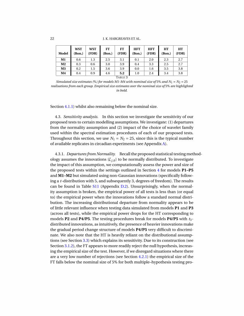
4.2.1. Discussion of findings. The empirical size values for models M1–M4
with N1 = N2 = 25 (this is the typical number of available replicates in circadian
experiments, see Appendix A) are reported in Table 3. The results for the HFT
with N1 = N2 = 1 are shown in Table S6, Appendix D.2 (recall: the HFT is the
only proposed test which can be applied when replicate data is not available–
see Section 3.2). The results for all tests with N1 = N2 = 10 and 50 replicates are
shown in Table S9 (Appendix D.2).
These studies show that the empirical size corresponding to all proposed tests
(apart from the FT for model M4 with N1 = N2 = 10 and 25) are less than the
nominal size of 5%. A close inspection of rejections for the FT for model M4 with
N1 = N2 = 10 and 25 and both multiple-hypothesis testing methods (Table S10
in Appendix D.2) reveals that, for this particular example, the number of rejec-
tions is often 1. If we disregard such situations, the empirical size of the FT also
falls below the nominal size of 5% for all sample sizes and multiple-hypothesis
testing procedures. In practice, circadian scientists are mostly interested in the
numbers of rejections and their locations and often choose to disregard situa-
tions where very few coefficients are significantly different. Indeed, this is also
our approach in Section 5.
Effect of Sample Size. Note that the tests scale well with increasing sample size,
with the nominal size acting as an upper bound, a behaviour also present in
other related empirical size investigations, see e.g. Cho (2016).
Approach to Multiple-hypothesis Testing. These studies show that the Bonfer-
roni correction provides a more conservative approach, whereas the false dis-
covery rate (using the correction outlined above) is closer to the nominal size.
Performance Comparison. The results for model M5 with N1 = N2 = 10 and
25 are shown in Table S8 (Appendix D.2). Note that the empirical size estimates
for our proposed tests are all lower than the nominal size of 5%, whereas for 10
replicates the empirical size of the ANT is 7.9%.
4.2.2. Size comparisons: Conclusions. These studies show that the empirical
size corresponding to all proposed tests is less than the nominal size of 5% (apart
from the FT for model M4 with N1 = N2 = 10 and 25– where, in most cases, the
number of significant coefficients was less than 5). We thus recommend using
the less conservative FDR procedure (ignoring situations with very small num-
bers of rejections). Note this also yields better results for empirical power (see
22 J. K. HARGREAVES ET AL.
Model
WST
(Bon.)
WST
(FDR)
FT
(Bon.)
FT
(FDR)
HFT
(Bon.)
HFT
(FDR)
HT
(Bon.)
HT
(FDR)
M1 0.6 1.3 2.5 3.1 0.1 2.0 2.3 2.7
M2 0.3 0.6 3.0 3.9 0.4 3.3 2.5 2.7
M3 0.2 1.5 3.6 3.9 0.0 1.6 3.5 3.8
M4 0.4 0.9 4.6 5.2 1.0 2.4 3.4 3.8
TABLE 3
Simulated size estimates (%) for models M1-M4 with nominal size of 5% and N1 = N2 = 25
realisations from each group. Empirical size estimates over the nominal size of 5% are highlighted
in bold.
Section 4.1.1) whilst also remaining below the nominal size.
4.3. Sensitivity analysis. In this section we investigate the sensitivity of our
proposed tests to certain modelling assumptions. We investigate: (1) departures
from the normality assumption and (2) impact of the choice of wavelet family
used within the spectral estimation procedures of each of our proposed tests.
Throughout this section, we use N1 = N2 = 25, since this is the typical number
of available replicates in circadian experiments (see Appendix A).
4.3.1. Departures from Normality. Recall the proposed statistical testing method-
ology assumes the innovations {ξ j ,k } to be normally distributed. To investigate
the impact of this assumption, we computationally assess the power and size of
the proposed tests within the settings outlined in Section 4 for models P1–P5
and M1–M2 but simulated using non-Gaussian innovations (specifically follow-
ing a t-distribution with 5, and subsequently 3, degrees of freedom). The results
can be found in Table S11 (Appendix D.2). Unsurprisingly, when the normal-
ity assumption is broken, the empirical power of all tests is less than (or equal
to) the empirical power when the innovations follow a standard normal distri-
bution. The increasing distributional departure from normality appears to be
of little relevant influence when testing data simulated from models P1 and P3
(across all tests), while the empirical power drops for the HT corresponding to
models P2 and P4/P5. The testing procedures break for models P4/P5 with t3-
distributed innovations, as intuitively, the presence of heavier innovations make
the gradual period change structure of models P4/P5 very difficult to discrimi-
nate. We also note that the HT is heavily reliant on the distributional assump-
tions (see Section 3.3) which explains its sensitivity. Due to its construction (see
Section 3.1.2), the FT appears to more readily reject the null hypothesis, increas-
ing the empirical size of the test. However, if we disregard situations where there
are a very low number of rejections (see Section 4.2.1) the empirical size of the
FT falls below the nominal size of 5% for both multiple–hypothesis testing pro-

WAVELET SPECTRAL TESTING FOR NONSTATIONARY CIRCADIAN RHYTHMS 23
cedures and all studies (other than M1 with FDR). We report here that the em-
pirical power of the ANT for model P1 (fixed spectra) with t-distributions with 5
degrees of freedom was 6.8%, which is below the results in Table S11 for all our
proposed tests (which are all over 99.9%). This is to be expected since, as in Sec-
tion 4.1, the underlying assumptions of the ANT are not valid. (Similar results
are obtained for models P2–P7, hence we do not provide these here.)
We also investigated the power and size for models P8–P12 and M5 (see Sec-
tion 4) simulated using non-Gaussian errors (specifically following t-distributions
with 5, and subsequently 3, degrees of freedom). The results can be found in Ta-
ble S12 (Appendix D.2). The WST, FT and HT appear to share a good degree of
robustness as they all have an empirical power over 99% for models P8–P11,
showing that our methodology can also be successfully applied to functional
time series (as designed for the ANT) with non-Gaussian error. Akin to the pre-
vious results for the gradual period change models P4/P5, the distribution of the
noise term does appear to have an adverse effect in model P12, where the dif-
ference between the periods of the two underlying signals is only 15 minutes.
Across this study, the HFT was most affected. A possible explanation is that the
HFT was constructed to detect differences in scale only and, due to the lower
frequency resolution of the wavelet spectrum, the total power within each scale
of the wavelet spectrum will be very similar for both groups. This issue will have
been compounded by the heavier tailed distribution of the noise term. We also
report here that, in the settings of this study, the performance of ANT was sus-
tained as its underlying assumptions are adhered to.
4.3.2. Choice of wavelet. The wavelet system gives a representation for non-
stationary time series under which we estimate the wavelet spectrum and subse-
quently perform hypothesis testing. We investigated the sensitivity of our meth-
ods to the wavelet choice. For models P1–P5, the Haar wavelet was used for
spectral estimation, but different, potentially mismatched wavelets were used
to generate the processes from the spectrum: Haar wavelets, Daubechies’ least-
asymmetric wavelets with 4 vanishing moments and Daubechies’ extremal phase
wavelets with 10 vanishing moments. Models P6–P12 were not generated from
LSW spectra (see Section 4), hence we report the results when using a selection
of wavelets for the empirical wavelet spectrum.
The results in Tables S13 and S14 (Appendix D.2) show that our methodology
is fairly robust to the wavelet choice. The empirical size estimates all fall below
the nominal size. The results indeed support the intuition that, as the scope of
our work is to devise tests that locally identify dissimilarities between pairs of
spectra, the short support overlaps of Haar wavelets counterbalance their oth-
erwise reduced capacity of representing smooth signals.

24 J. K. HARGREAVES ET AL.
4.4. Summary of findings. A summary of the hypothesis tests developed in
this manuscript detailing the test name, its acronym, strengths and weaknesses
can be found in Table S15 (Appendix E).
5. Real data analysis: back to the motivating circadian datasets. We now
use our proposed methodology to analyse the motivating examples (Section 1).
Prior to analysis, we investigate whether the normality assumption is tenable
for each of our motivating datasets. The results (Appendix B.2) show that, for
each of our motivating datasets, the normality assumption is appropriate. We
then model each circadian trace as a (Gaussian) LSW process, estimate its cor-
responding group wavelet spectral representation and consequently construct
the appropriate test statistic that aims to identify whether a departure towards a
specific type of spectral difference is present or not (as described in Section 3).
For each dataset, the corresponding number of rejections can be found in Table
S3 (Appendix B.1), with corresponding representative ‘barcode’ plots in Figures
4, 5 and 6.
We also note here that the data naturally shared the same starting point and
had the same length (see Appendix A). Therefore, instances where these condi-
tions are not satisfied are not the focus of this paper and we leave these issues
for future research.
5.1. Lead dataset. Section 1.1.1 outlined the scientific aims to determine if
lead nitrate affects the circadian clock and, if so, to detect the times and scales
at which any significant differences arise between the ‘Control’ and ‘Lead’ ex-
posure groups. Therefore we are particularly interested in the results of the FT.
Table S3 shows the results for the FT and includes both the more conservative
Bonferroni correction and FDR. In order to visualise the areas of null hypothe-
sis rejection of spectral equality between the control and lead-exposure groups,
both group average estimated spectra as well as the ‘barcode’ plot for the FT
(with FDR) appear in Figure 4. Figure 4 indicates that the differences between
the two spectra lie in resolution levels 2–4, directly corresponding to a circadian
rhythm, with the number of rejections increasing with exposure time. We con-
clude that there is evidence that exposure to lead does affect the circadian clock
of A. thaliana, and this change manifests itself after approximately three days of
free-running conditions.
5.2. Ultradian dataset. Section 1.1.2 introduced this experiment and high-
lighted the need to detect whether any differences appear in the circadian and
ultradian components of the ‘Control’ and ‘Mutant’ groups. Hence we are in-
terested in the results of the HFT, specifically developed to identify the scales,
rather than the times, at which potential differences arise. Table S3 shows the

WAVELET SPECTRAL TESTING FOR NONSTATIONARY CIRCADIAN RHYTHMS 25
FIG 4. Lead dataset. Left: Average estimated spectrum of the ‘Control’ group; Centre: Average esti-
mated spectrum of the ‘Lead’ group; Right: ‘Barcode’ plot for FT (with FDR).
results for the HFT, including both the Bonferroni correction and FDR. The re-
sults indicate rejections of the null hypothesis of spectral equality between the
control and mutant plants across a range of scales. The group average estimated
spectra and ‘barcode’ plot for the HFT (with FDR) can be found in Figure 5. Note
that the differences between the two spectra lie in the coarsest resolution levels
1–4, associated with circadian rhythms, and higher-frequency levels 6 and 7, cor-
responding to an ultradian rhythm. We conclude that there is evidence that the
mutant plants have altered circadian and ultradian rhythms within A. thaliana.
5.3. Nematode dataset. The experiment in Section 1.1.3 aimed to elucidate
the effect of a pharmacological treatment on the C. elegans clock. The average
estimated spectra of the ‘Control’ and ‘Treatment’ groups in Figure 6 share a
common profile but with differences in magnitude, indicating that the HT would
be appropriate in this context. Table S3 shows that the HT found no significant
difference between the shapes of the two spectra, but when tested for equal-
ity, the FT (with FDR) found multiple rejections of the null hypothesis of spec-
tral equality between the ‘Control’ and ‘Treatment’ groups (refer to the ‘barcode’
plot in Figure 6). This provides evidence that the two spectra have the same pro-
file within each scale up to an additive non-zero constant. We thus conclude
that there is evidence that the treatment significantly affects the intensity of the
spectral behaviour, but not its pattern. The spectral differences are present at
the highest frequencies (resolution levels 6–8) as an early response to the onset
of treatment (prior to time T = 48), see Figure 6.

26 J. K. HARGREAVES ET AL.
FIG 5. Ultradian dataset. Left: Average estimated spectrum of the ‘Control’ group; Centre: Average
estimated spectrum of the ‘Mutant’ group; Right: ‘Barcode’ plot for HFT (with FDR).
FIG 6. Nematode dataset. Left: Average estimated spectrum of the ‘Control’ group; Centre: Average
estimated spectrum of the ‘Treatment’ group; Right: ‘Barcode’ plot for FT (with FDR).

WAVELET SPECTRAL TESTING FOR NONSTATIONARY CIRCADIAN RHYTHMS 27
5.4. Discussion of results. Overall, we recall that, for each of our motivating
datasets, the established Fourier-based tests currently adopted within the circa-
dian community found no significant difference between the groups (see Table
S1 in Appendix B.1), even though qualitative differences are easily noted (see
Section 1.1). This methodology assumes data stationarity, but for our motivat-
ing datasets we have shown that this assumption is not appropriate (see Table S2
in Appendix B.1). Our proposed methodology was able to detect the visually ap-
parent differences between the motivating datasets when the current method-
ology could not (see Tables S3 and S1 in Appendix B.1). Due to the nonstationary
character of the proposed approach, it also additionally indicates precise times
and/or scales at which differences become manifest.
6. Conclusions and further work. This work was stimulated by a variety
of challenging applications faced by the circadian–biology community, which
is becoming increasingly aware of the nonstationary characteristics present in
much of their data (Hargreaves et al., 2018; Zielinski et al., 2014; Leise et al.,
2013). Our methodology fills the gap in the current literature by developing and
testing much needed tools for the formal spectral comparison of nonstation-
ary data. Our methods are developed as testing procedures, analogous to the
period analysis techniques currently adopted within the circadian community.
Motivated by three complementary applications in circadian biology, our new
methodology allows the identification of three specific types of spectral differ-
ence. Table S15 in Appendix E provides a summary of the hypothesis tests devel-
oped in this manuscript detailing their strengths and weaknesses.
The competitive performance of our methods was comparatively assessed in
an extensive simulation study (Section 4). Additionally, when compared to exist-
ing methods currently adopted within the circadian community, our proposed
tests were able to discriminate between real data sets (Table S3) where the cur-
rent methodology could not (Table S1).
In the applications provided, we illustrated the important implications in fur-
ther understanding the mechanisms behind the plant and nematode circadian
clocks, and the environmental implications associated with soil pollution. How-
ever, we note that our methodology can readily be applied to other circadian
datasets, as well as to data originating in other fields, as long as the data share
the same dyadic length (T ). This assumption is easily achievable for most exper-
imental data, but for other setups might necessitate further specific treatments
depending on the discrepancy between the number of observations.
In all of our proposed hypothesis tests, we wish to test many hypotheses of the
type H0 : S(1)j
(k/T ) = S(2)j
(k/T ) for several values of j and k. In this manuscript
we tested the Bonferroni correction and, for a less conservative approach, the

28 J. K. HARGREAVES ET AL.
false discovery rate (FDR) procedure. We recommend the use of the FDR proce-
dure, as this gave a higher empirical power and was closer to the nominal size in
the simulation studies (see Section 4). However, the multiple-hypothesis testing
methods we use do not account for the dependence of the spectral coefficients.
The hypothesis tests developed in Sections 3.2 and 3.3 alleviate this problem
by transforming the data to produce coefficients that are approximately uncor-
related but, as neither method fully decorrelates the data, multiple-hypothesis
testing methods that take the dependence of the (transformed) spectral coeffi-
cients into account are an interesting avenue of further work.
APPENDIX A: EXPERIMENTAL DETAILS
In this section we outline the experimental details that led to the datasets in-
troduced in Section 1.1 and subsequently analysed in Sections 5.1, 5.2 and 5.3.
Experimental overview: Lead and Ultradian Datasets. Both Davis and Millar labs
used a firefly luciferase reporter system. This involves fusing the gene of interest
(here, ‘cold and circadian regulated and RNA binding 2’, CCR2) to a biolumines-
cent enzyme called luciferase (Doyle et al., 2002). When CCR2 is expressed, the
resultant luciferase emits light which is measured using a TopCount NXT scin-
tillation counter (Perkin Elmer), allowing relative gene expression of CCR2 to be
quantified in vivo (Southern and Millar, 2005; Perea-García et al., 2015).
Lead nitrate dataset. Arabidopsis thaliana seeds (Ws–CCR2:LUC (Doyle et al.,
2002)) were surface sterilised and plated onto Hoagland’s media containing 1%
sucrose, 1.5% phyto agar (Hoagland et al., 1950). The seeds were stratified for 2
days at 4◦C and transferred to growth chambers to entrain under 12:12 light/dark
cycles at a constant temperature of 20◦C. Six-day-old seedlings were transferred
to 96 well microtiter plates containing Hoagland’s 1% sucrose, 1.5% agar (Hanano
et al., 2006) with or without supplemental Pb(NO3)2 (lead nitrate) at a concen-
tration of 1.4mM. After 24 hours, the plants were then transferred to the TOP-
Count machine. Measurements were taken at intervals of approximately 45 min-
utes. Measurement began after the transition to 12 hours of darkness (known as
subjective dusk) on the seventh day of the plants’ life. Therefore, the plants ex-
perience one ‘normal’ day in the TOPCount machine (known as entrainment).
After this, the plants are exposed to constant light (known as an LL free-run)
for approximately four days. This dataset consists of 48 plant signals recorded
at T = 128 time points, with both the ‘Control’ and ‘Lead’ groups containing 24
plants.
Ultradian dataset. (Millar et al., 2015). This dataset was obtained following a
similar method as outlined for the Lead dataset above, but compared ‘Control’
A. thaliana plants (Ws–2 with CCR2:LUC (Doyle et al., 2002)) with ‘Mutant’ A.
thaliana plants (Ws–2 cca1 lhy). Plants were grown on MS media Murashige and

WAVELET SPECTRAL TESTING FOR NONSTATIONARY CIRCADIAN RHYTHMS 29
Dataset
Mean Period Estimate:
Control Group
Mean Period Estimate:
Test Group Difference p–value
Lead 27.4 26.8 -0.6 0.16
Ultradian 6.5 6.5 0.0 0.98
Nematode 24.8 25.6 +0.8 0.55
TABLE S1
A summary of the output of the analysis of the motivating example datasets in BRASS: the mean
period estimate for the control and test groups in hours (obtained using FFT-NLLS analysis (Plautz
et al., 1997)), the difference between the period estimates and the corresponding p–value.
Skoog (1962) with 3% sucrose and 1.5% phyto-agar. Plants were entrained in
12:12 L:D conditions at 22◦C followed by an LL free-run. Measurements were
taken at intervals of approximately 30 minutes. This dataset consists of 48 plant
signals recorded at T = 256 time points, with both the ‘Control’ and ‘Mutant’
groups containing 24 plants.
Nematode dataset. This dataset was obtained using male Caenorhabditis ele-
gans strain PE254 (obtained from the CGC), which expresses firefly luciferase
under the promoter of the sur-5 gene (feIs4 [Psur-5::luc+::gfp; rol-6(su1006)] Lagido
et al. (2008)). Nematodes expressing luciferase driven by the sur-5 promoter
have previously been reported to show circadian rhythms in luminescence (Goya
et al., 2016). Single nematodes were placed in wells containing 100µl S buffer
(Stiernagle, 1999), supplemented with 5 mg/mL cholesterol, 1 g/L wet weight
pelleted Escherichia coli OP50 strain and 100 µM luciferin. Treatment wells also
contained 10 µM SB 203580 (a p38 MAPK inhibitor (Sigma S8307)). Entrainment
conditions were 12 hours at 20◦C followed by 12 hours at 15◦C for two days in
constant darkness. Free-running was at 20◦C in constant darkness. Luciferase
measurements were recorded approximately every 13 minutes. Nematodes that
died (shown by a sudden loss of luciferase expression) were excluded from data
analysis. Therefore, this dataset consists of 62 signals recorded at T = 512 time
points, with the ‘Control’ and ‘Treatment’ groups containing 32 and 30 time se-
ries respectively.
APPENDIX B: REAL DATA ANALYSIS: SUPPLEMENTARY MATERIAL
B.1. Supplementary Tables. In this section, for each motivating example
dataset, we report: a summary of the output of the analysis of the motivating
datasets in BRASS (Table S1); the results of the Priestley-Subba Rao test of sta-
tionarity (for each time series) in Table S2 and the number of rejections for the
relevant proposed hypothesis testing procedure (Table S3).

30 J. K. HARGREAVES ET AL.
Dataset Lead Ultradian Nematode
Number of nonstationary time series 39 (81%) 41 (85%) 61 (98%)
Total number of time series 48 48 62
TABLE S2
Results for the Priestley-Subba Rao test of stationarity, implemented in the fractal package in R
and available from the CRAN package repository. Number of nonstationary plants indicates the
number of time series (in each motivating example dataset) with enough evidence to reject the null
hypothesis of stationarity at the 5% significance level (as a percentage in brackets).
Dataset (Test) Bon. FDR
Lead (FT) 31 (3%) 133 (15%)
Ultradian (HFT) 1102 (54%) 1538 (75%)
Nematode (HT) 0 (0%) 0 (0%)
TABLE S3
The number of rejections (as a percentage in brackets) for each relevant proposed test and
multiple-hypothesis testing procedure for the motivating example datasets.
B.2. Tenability of the Normality Assumption. In this section we investigate
the tenability of the normality assumption for each of our motivating datasets.
Following Fryzlewicz (2005), for each series, we standardise the (zero-mean) data
using an estimate of the local standard deviation. The estimate was obtained by
means of a localised a Gaussian kernel with bandwidth chosen using the meth-
ods of Fryzlewicz (2005). We then examine the Q–Q plot of the standardised se-
ries against the normal quantiles. We report Q–Q plots for a representative series
from the control and test groups of each of our motivating datasets in Figure
S1. These demonstrate that the normality assumption holds for our motivat-
ing data, an assumption also typically undertaken by the circadian community
(Perea-García et al., 2015).
APPENDIX C: BACKGROUND FOR LOCALLY STATIONARY WAVELET (LSW)
PROCESSES
In this section we provide the technical details that underline the LSW process
model introduced by Nason et al. (2000).
The locally stationary wavelet processes are a sequence of doubly indexed
stochastic processes {X t ,T }t=0,...,T−1, T = 2J ≥ 1, having the representation in the
mean-square sense
(C.1) X t ,T =
J∑
j=1
∑
k
w j ,k;T ψ j ,k (t )ξ j ,k ,
where ξ j ,k is a random orthonormal increment sequence and where {ψ j ,k (t )} j ,k

WAVELET SPECTRAL TESTING FOR NONSTATIONARY CIRCADIAN RHYTHMS 31
FIG S1. Q–Q plots for a representative series from the control (Plots A, C, E) and test groups (Plots B,
D, F) of each of our motivating datasets. Lead Dataset: Plots A and B. Ultradian Dataset: C and D.
Nematode Dataset: E and F.
is a discrete non-decimated family of wavelets based on a mother waveletψ(t ) of
compact support. The quantities in equation (C.1) have the following properties:
(a) E(ξ j ,k ) = 0 for all j ,k. Hence E(X t ,T ) = 0 for all t ,T ,
(b) Cov(ξ j ,k ,ξℓ,m) = δ j ,ℓδk,m where δi , j is the Kronecker delta.
(c) There exists, for each j ≥ 1 a Lipschitz continuous function W j (z) for z ∈
(0,1) which fulfils the following properties:
∞∑
j=1
|W j (z)|2 <∞ uniformly in z ∈ (0,1);
the Lipschitz constants L j are uniformly bounded in j and
∞∑
j=1
2 j L j <∞;
there exists a sequence of constant C j such that for each T
supk
∣
∣w j ,k;T −W j (k/T )∣
∣≤C j /T,
where {C j } fulfils∑∞
j=1 C j <∞.
The (evolutionary) wavelet spectrum is defined as S j (z) = |W j (z)|2 at scale j
and rescaled time z = t/T , and is connected to a localised autocovariance func-
tion defined for each (rescaled) time z and lag τ as follows
(C.2) c(z,τ) =∞∑
j=1
S j (z)Ψ j (τ).

32 J. K. HARGREAVES ET AL.
In the above, the quantities {Ψ j (τ)} j define a family of locally supported auto-
correlation wavelets that can deliver sparse representations (Nason et al., 2000).
Once a well-behaved spectral estimator has been obtained, equation C.2 can be
used to obtain a local autocovariance estimator c(z,τ) and its approximate con-
fidence bounds, under the assumption of Gaussian innovations (Nason, 2013).
APPENDIX D: DETAILED DESCRIPTION OF SIMULATION STUDIES
In this section we give a more detailed description of the simulation studies
outlined in Section 4. The basic structure of each simulated experiment can be
described as follows. In each case, we assumed that the signal was a realisation
of length T = 256 from one of i = 1,2 possible groups, each having (possibly)
different spectral structure. A set of N1 = N2 = 1,10,25,50 signal realisations for
each group was generated either from variously defined: spectra (models P1–P5
and M1 and M2); AR processes (models P6, P7, M3 and M4) or functional time
series (models P8–P12 and M5).
For the models defined by group spectra, signal realisations were generated
using the locits package in R (available from the CRAN package repository)
and the representation in equation (2.2) with (unless otherwise stated) the Haar
wavelet and a Gaussian orthonormal increment sequence with mean zero and
unit variance. (Note that the wavethresh package in R preceded the locits
package and can also be used to generate LSW processes. For more informa-
tion on how to generate LSW processes from a particular spectrum see Nason
(2010).)
D.1. Model Details. In this section we give a detailed description of each
model outlined in Sections 4.1 and 4.2.
1. P1: Fixed Spectra. We follow Krzemieniewska et al. (2014) Section 4.1.1-
Fixed spectra where the spectra of the two groups differ only at the finest
level by 100 coefficients. We simulate each replicate ri -th time series of
length T = 256 of the i -th group from the wavelet spectrum {S(i )j
(z)}Jj=1
which we define for each of the i = 1,2 groups as follows:
(D.1) S(1)j
(z) =
4cos2(2πz), for j = 3, z ∈ (0,1)
1, for j = 7, z ∈ (1/256,56/256)
0, otherwise;
and
(D.2) S(2)j
(z) =
4cos2(2πz), for j = 3, z ∈ (0,1)
1, for j = 7, z ∈ (1/256,156/256)
0, otherwise.

WAVELET SPECTRAL TESTING FOR NONSTATIONARY CIRCADIAN RHYTHMS 33
FIG S2. P1:Fixed Spectra. Top left: Group 1 wavelet spectrum; Top right: Group 2 wavelet spectrum;
Bottom left: Group 1 realisation; Bottom right: Group 2 realisation.
Figure S2 provides a visualisation of the wavelet spectra (top row) and an
example of a signal realisation from each of the two groups (bottom row).
2. P2: Fixed Spectra-Fine Difference. For our next study, we modify the set-
ting above such that the spectra of the two groups differ by 6 coefficients
(in resolution level 7). Therefore, {S(1)j
(z)}Jj=1
is as defined in equation (D.1)
above but we specify the evolutionary wavelet spectrum {S(2)j
(z)}Jj=1
as fol-
lows:
(D.3) S(2)j
(z) =
4cos2(2πz), for j = 3, z ∈ (0,1)
1, for j = 7, z ∈ (1/256,50/256)
0, otherwise.
Figure S3 provides a visualisation of the wavelet spectra (top row) and an
example of a signal realisation from each of the two groups (bottom row).
3. P3: Fixed Spectra-Plus Constant. We now define fixed spectra such that
the spectra of the two groups differ by a constant at the finest resolution
level. Therefore, {S(1)j
(z)}Jj=1
is as defined in equation (D.1) above but we
specify the evolutionary wavelet spectrum {S(2)j
(z)}Jj=1
as follows:
(D.4) S(2)j
(z) =
4cos2(2πz), for j = 3, z ∈ (0,1)
2, for j = 7, z ∈ (1/256,56/256)
1, for j = 7, z ∈ (57/256,256/256)
0, otherwise.

34 J. K. HARGREAVES ET AL.
FIG S3. P2:Fixed Spectra-Fine Difference. Top left: Group 1 wavelet spectrum; Top right: Group 2
wavelet spectrum; Bottom left: Group 1 realisation; Bottom right: Group 2 realisation.
Figure S4 provides a visualisation of the wavelet spectra (top row) and an
example of a signal realisation from each of the two groups.
4. P4/P5: Gradual Period Change. With this simulation study aiming to repli-
cate a typical circadian experiment with changes beyond the stationar-
ity assumption, we define time series as realisations from one of 3 possi-
ble groups, each with different spectral characteristics. In particular, each
group represents a time series that gradually changes period from 24 to:
25 (Group 1), 26 (Group 2) and 27 (Group 3) over (approximately) two
days, before continuing with the relevant period for a further two days.
We choose T = 256 which is equivalent to a free-running period of 4 days
with equally spaced observations every 22.5 minutes. Figure S5 shows the
wavelet spectra which display the gradually changing periods that define
each of the 3 groups. (Note that the increased period is shown by the move-
ment up through the resolution levels and the gradual increase in period
of the wavelet coefficients.) To determine which changes can be discrimi-
nated by the methods, we perform two studies within this setting: P4: sim-
ulations from Group 1 and Group 2 and P5: simulations from Group 1 and
Group 3.
5. P6/P7: AR Processes with Time-Varying Coefficients. The signals in mod-
els P1–P5 are generated from a defined group spectrum, satisfying the
underlying LSW modelling assumptions of our proposed tests. The pur-
pose of this study is to asses the performance of our tests when these as-
sumptions are not met. Therefore, we simulate from an important class

WAVELET SPECTRAL TESTING FOR NONSTATIONARY CIRCADIAN RHYTHMS 35
FIG S4. P3:Fixed Spectra-Plus Constant. Top left: Group 1 wavelet spectrum; Top right: Group 2
wavelet spectrum; Bottom left: Group 1 realisation; Bottom right: Group 2 realisation.
FIG S5. P4/P5: Gradual Period Change. Left: Group 1 wavelet spectrum (gradual period change
from 24 to 25 hours); Centre: Group 2 wavelet spectrum (gradual period change from 24 to 26
hours); Right: Group 3 wavelet spectrum (gradual period change from 24 to 27 hours).

36 J. K. HARGREAVES ET AL.
Time-varying parameters Time Index Group i = 1 Group i = 2
φ(i )1 (t ) t = 1, . . . ,53 0.8 0.8
t = 54, . . . ,128 -0.9 -0.3
t = 129, . . . ,256 0.8 0.8
φ(i )2 (t ) t = 1, . . . ,256 -0.81 -0.81
TABLE S4
P6: AR Processes with Abruptly Changing Parameters. The abruptly changing parameters of two
nonstationary autoregressive processes.
of nonstationary processes– AR processes with time-varying coefficients.
We propose a simulation study in a setting as described in Fryzlewicz and
Ombao (2009) Section 4.1 Cases 1 and 2.
P6: AR Processes with Abruptly Changing Parameters. The ri -th time se-
ries from group i = 1,2, denoted X(i ),ri
n,t is generated from the process de-
fined by:
(D.5) X(i ),ri
t =φ(i )1 (t )X
(i ),ri
t−1 +φ(i )2 (t )X
(i ),ri
t−2 +ǫ(i ),ri
t ,
where the innovations ǫ(i ),ri
t are independent and identically distributed
(iid) Gaussian with zero mean and unit variance. In this study, the squared
difference between the group spectra is relatively small and the abruptly
changing parameters for the two groups are shown in Table S4. Repre-
sentative time series plots from each group and the estimated spectra are
shown in Figure S6.
P7: AR Processes With Slowly Changing Parameters. The ri -th time series
from group i = 1,2, denoted X(i ),ri
t is generated from the process defined
by:
(D.6) X(i ),ri
t =φ(i )1 (t )X
(i ),ri
t−1 +φ(i )2 (t )X
(i ),ri
t−2 +ǫ(i ),ri
t ,
where the innovations ǫ(i ),ri
t are iid Gaussian with zero mean and unit
variance. In this study, the group wavelet spectra are highly similar and
hence the squared difference between group spectra is relatively small.
The slowly changing parameters for groups i = 1,2 are shown in Table S5.
Representative time series plots from each group and the estimated spec-
tra are shown in Figure S7.
6. P8–P12: Functional Time Series (Constant Period). This study follows
Zielinski et al. (2014) and generates each time series using an underlying
cosine curve with additive noise, which also coincides with the theoreti-
cal assumptions of the ANT. As in Models P4 and P5, we choose T = 256,
which is equivalent to a free-running period of 4 days with equally spaced

WAVELET SPECTRAL TESTING FOR NONSTATIONARY CIRCADIAN RHYTHMS 37
FIG S6. P6: AR Processes with Abruptly Changing Parameters. Nonstationary autoregressive pro-
cesses. Top left: Estimated wavelet spectrum of Group 1; Top right: Estimated wavelet spectrum of
Group 2; Bottom left: Group 1 realisation; Bottom right: Group 2 realisation.
Time-varying parameters Group i = 1 Group i = 2
φ(i )1 (t ) −0.8[1−0.7cos(πt/T )] −0.8[1−0.1cos(πt/T )]
φ(i )2 (t ) -0.81 -0.81
TABLE S5
P7: AR Processes With Slowly Changing Parameters. The slowly changing parameters of two
nonstationary autoregressive processes.
FIG S7. P7: AR Processes with Slowly Changing Parameters. Top left: Estimated wavelet spectrum
of Group 1; Top right: Estimated wavelet spectrum of Group 2; Bottom left: Group 1 realisation;
Bottom right: Group 2 realisation.

38 J. K. HARGREAVES ET AL.
FIG S8. P10: Functional Time Series with Constant Period. Top left: Estimated wavelet spectrum
of Group 1 (24 hour period); Top right: Estimated wavelet spectrum of Group 4 (23 hour period);
Bottom left: Group 1 realisation; Bottom right: Group 4 realisation. Grey lines indicate a 24 hour
period.
observations every 22.5 minutes. The ri -th time series from group i = 1,2,
denoted X(i ),ri
t is generated from the process defined by:
(D.7) X(i ),ri
t = f (i )(t )+ǫ(i ),ri
t ,
where the random variables ǫ(i ),ri
t are iid Gaussian with zero mean and
unit variance and the functions f (i )(t ) are defined below. We define time
series as realisations from one of 6 possible groups, each with a differ-
ent (constant) period. The function f (i )(t ) is set as a cosine curve with
an amplitude of 2 and a period of: 24 hours (Group 1), 21 hours (Group
2), 22 hours (Group 3), 23 hours (Group 4), 23.5 hours (Group 5) and 23.75
hours (Group 6). Representative time series plots and the estimated spec-
tra for Groups 1 and 4 are shown in Figure S8. To determine which period
changes can be discriminated by the methods, we perform five studies
within this setting: simulations from Group 1 and Groups 2–6 (models P8–
P12 respectively).
D.2. Supplementary Tables. In this section we provide results which sup-
port the discussion of the hypothesis tests in Section 4. We report the simulated
power and size estimates for N1 = N2 = 1,10,50 for the simulation studies out-
lined in Sections 4.1 and 4.2 in tables S6 – S9. Additionally, we report the num-
ber of rejections for the FT for model M4 with N1 = N2 = 10 and 25 and both
multiple-hypothesis testing methods in Table S10.

WAVELET SPECTRAL TESTING FOR NONSTATIONARY CIRCADIAN RHYTHMS 39
Model P1 P2 P3 P4 P5 P6 P7 M1 M2 M3 M4
HFT
(Bon.) 69.4 3.8 72.6 4.1 51.3 2.5 21.8 2.8 4.1 0.8 1.5
HFT
(FDR) 77.7 4.9 79.0 5.4 57.9 15.2 35.9 3.2 4.8 1.7 2.1
TABLE S6
Simulated power and size estimates (%) for the HFT for models P1-P7 and M1-M4 with nominal
size of 5% and N1 = N2 = 1 realisation from each group.
N Model
WST
(Bon.)
WST
(FDR)
FT
(Bon.)
FT
(FDR)
HFT
(Bon.)
HFT
(FDR)
HT
(Bon.)
HT
(FDR)
10 P1 100.0 100.0 100.0 100.0 100.0 100.0 100.0 100.0
10 P2 3.5 4.6 51.9 54.3 4.1 6.5 16.9 17.4
10 P3 100.0 100.0 100.0 100.0 100.0 100.0 4.2 4.3
10 P4 0.5 0.6 8.4 10.8 4.8 7.0 50.4 55.4
10 P5 0.4 1.1 22.6 31.0 73.4 80.2 95.8 98.4
10 P6 92.2 99.7 14.7 16.4 3.4 30.7 11.6 12.2
10 P7 99.2 100.0 11.5 12.1 30.0 54.7 75.6 77.4
50 P1 100.0 100.0 100.0 100.0 100.0 100.0 100.0 100.0
50 P2 94.8 97.2 100.0 100.0 87.1 88.5 100.0 100.0
50 P3 100.0 100.0 100.0 100.0 100.0 100.0 5.3 5.3
50 P4 11.8 28.0 96.0 99.0 92.0 94.8 100.0 100.0
50 P5 60.2 86.6 100.0 100.0 100.0 100.0 100.0 100.0
50 P6 100.0 100.0 100.0 100.0 96.7 100.0 99.3 99.8
50 P7 100.0 100.0 99.0 100.0 100.0 100.0 100.0 100.0
TABLE S7
Simulated power estimates (%) for models P1-P7 with nominal size of 5%. N = N1 = N2 is the
number of realisations in each group. Highest empirical power estimates are highlighted in bold.
We also report the simulated power and size estimates for N1 = N2 = 25 for the
simulation studies outlined in: Section 4.3.1 in Tables S11 and S12 and Section
4.3.2 in Tables S13 and S14.
APPENDIX E: SUMMARY TABLE
Table S15 provides a summary of the hypothesis tests developed in this manuscript
detailing the test name, its acronym, strengths and weaknesses for each of the
proposed tests.
REFERENCES
Atkinson, A. D., Hill, R. R., Pignatiello Jr, J. J., Vining, G. G., White, E. D. and Chicken, E. (2017).
Wavelet ANOVA approach to model validation. Simulation Modelling Practice and Theory,
78:18–27.

40 J. K. HARGREAVES ET AL.
N Model
Test Group
Period
WST
(FDR)
FT
(FDR)
HFT
(FDR)
HT
(FDR) ANT
10 P8 21 100.0 100.0 100.0 100.0 100.0
10 P9 22 100.0 100.0 93.3 100.0 100.0
10 P10 23 100.0 100.0 31.9 100.0 100.0
10 P11 23.5 100 96.1 9.5 99.4 100.0
10 P12 23.75 81.2 14.6 5.6 32.4 100.0
10 M5 24 2.0 2.1 3.1 4.1 7.9
25 M5 24 3.0 2.7 2.7 3.5 4.8
TABLE S8
Simulated size and power estimates (%) for models P8-P12 and M5 with nominal size of 5% and
using the false discovery rate procedure (FDR). N = N1 = N2 is the number of realisations in each
group. Note: Control group period is 24 hours in each model.
N Model
WST
(Bon.)
WST
(FDR)
FT
(Bon.)
FT
(FDR)
HFT
(Bon.)
HFT
(FDR)
HT
(Bon.)
HT
(FDR)
10 M1 0.3 0.5 2.6 3.3 1.0 2.6 2.5 2.7
10 M2 0.0 0.2 2.4 3.6 2.0 5.0 3.3 3.3
10 M3 0.3 1.2 4.1 4.4 0.2 1.4 1.9 2.1
10 M4 0.4 1.6 5.1 5.6 0.9 1.8 2.1 2.2
50 M1 0.4 1.1 2.4 3.9 0.3 2.4 3.1 3.3
50 M2 0.3 0.6 3.1 3.8 1.4 3.1 2.5 2.6
50 M3 0.5 1.2 4.4 4.8 0.2 2.2 3.9 4.2
50 M4 0.2 1.1 4.4 4.8 1.3 2.6 2.8 2.9
TABLE S9
Simulated size estimates (%) for models M1-M4 with nominal size of 5%. N = N1 = N2 is the
number of realisations in each group. Empirical size estimates over the nominal size of 5% are
highlighted in bold.
N
Multiple-hypothesis
Testing Method
1
Rej.
2
Rej.
3
Rej.
4
Rej.
>5
Rej.
Modified Empirical
Size Estimate
10 Bon. 44 5 2 0 0 0.7
10 FDR 40 12 3 0 1 1.6
25 Bon. 38 8 0 0 0 0.8
25 FDR 31 16 3 2 0 2.1
50 Bon. 39 5 0 0 0 0.5
50 FDR 32 10 3 0 3 1.6
TABLE S10
M4: AR Process with Slowly Changing Parameters. Numbers of rejections in empirical size
estimates for the Raw Periodogram F-Test (FT), with Bonferroni Correction (Bon.) and false
discovery rate (FDR) and with nominal size of 5%. “Modified Empirical Size Estimate” is calculated
by examining only cases with more than one significant coefficient.

WAVELET SPECTRAL TESTING FOR NONSTATIONARY CIRCADIAN RHYTHMS 41
Model Test N(0,1) t5 t3
P1 WST 100.0 100.0 100.0
P1 FT 100.0 100.0 100.0
P1 HFT 100.0 99.9 88.4
P1 HT 100.0 100.0 93.3
P2 WST 48.0 30.5 11.6
P2 FT 100.0 100.0 100.0
P2 HFT 31.8 5.6 1.6
P2 HT 86.4 53.5 17.9
P3 WST 100.0 100.0 100.0
P3 FT 100.0 100.0 100.0
P3 HFT 100.0 100.0 97.0
P3 HT 4.4 2.4 1.9
P4 WST 2.7 1.2 0.6
P4 FT 54.5 49.1 35.7
P4 HFT 36.5 4.7 4.0
P4 HT 100.0 79.7 40.0
P5 WST 14.6 1.1 0.3
P5 FT 99.9 76.6 32.9
P5 HFT 100.0 30.1 11.3
P5 HT 100.0 81.6 38.4
M1 WST 1.3 0.7 0.1
M1 FT 3.1 4.1 14.5
M1 HFT 2.0 3.2 1.8
M1 HT 2.7 2.7 0.6
M2 WST 0.6 0.1 0.4
M2 FT 3.9 4.5 4.5
M2 HFT 3.3 2.9 2.1
M2 HT 2.7 0.9 0.9
TABLE S11
Potential Non-Gaussian Innovations: Simulated size and power estimates (%) for models P1-P5
and M1, M2 with nominal size of 5% and N1 = N2 = 25 realisations from each group. Innovations
are distributed as: standard normal (denoted N(0,1)) or t-distribution with 5 or 3 degrees of
freedom (denoted t5, t3 respectively). For the FT, the modified size and power estimates are
recorded (i.e. only consider cases when more than 5 rejections are reported– see Section 4.2).
Empirical size estimates over the nominal size of 5% are highlighted in bold.

42 J. K. HARGREAVES ET AL.
Model Test N(0,1) t5 t3
P8 WST 100.0 100.0 100.0
P8 FT 100.0 100.0 100.0
P8 HFT 100.0 100.0 99.6
P8 HT 100.0 100.0 100.0
P9 WST 100.0 100.0 100.0
P9 FT 100.0 100.0 100.0
P9 HFT 100.0 99.9 79.4
P9 HT 100.0 100.0 100.0
P10 WST 100.0 100.0 100.0
P10 FT 100.0 100.0 100.0
P10 HFT 92.0 59.5 25.6
P10 HT 100.0 100.0 100.0
P11 WST 100.0 100.0 100.0
P11 FT 100.0 100.0 100.0
P11 HFT 31.8 15.1 8.1
P11 HT 100.0 100.0 99.5
P12 WST 100.0 98.5 52.4
P12 FT 97.9 83.6 80.0
P12 HFT 9.1 5.9 3.6
P12 HT 98.3 77.2 31.6
M5 WST 3.0 1.0 1.5
M5 FT 2.7 1.7 10.4
M5 HFT 2.7 2.0 0.9
M5 HT 3.5 4.2 1.5
TABLE S12
Potential Non-Gaussian Errors: Simulated size and power estimates (%) for models P8-P12 and
M5 with nominal size of 5% and N1 = N2 = 25 realisations from each group. The noise term in
equation (D.7) is distributed as: standard normal (denoted N(0,1)) or t-distribution with 5 or 3
degrees of freedom (denoted t5, t3 respectively). For the FT, the modified size and power estimates
are recorded (i.e. only consider cases when more than 5 rejections are reported– see Section 4.2).
Empirical size estimates over the nominal size of 5% are highlighted in bold.

WAVELET SPECTRAL TESTING FOR NONSTATIONARY CIRCADIAN RHYTHMS 43
Model Test
Haar
wavelet
(1 V.M.)
Daubechies’
least-asymmetric
(4 V.M.)
Daubechies’
extremal phase
(10 V.M.)
P1 WST 100.0 100.0 100.0
P1 FT 100.0 100.0 100.0
P1 HFT 100.0 100.0 100.0
P1 HT 100.0 100.0 100.0
P2 WST 48.0 55.7 44.6
P2 FT 100.0 100.0 100.0
P2 HFT 31.8 78.2 73.9
P2 HT 86.4 99.9 99.6
P3 WST 100.0 100.0 100.0
P3 FT 100.0 100.0 100.0
P3 HFT 100.0 100.0 100.0
P3 HT 4.4 4.2 6.0
P4 WST 2.7 23.5 25.1
P4 FT 54.5 91.9 89.4
P4 HFT 36.5 96.5 78.0
P4 HT 100.0 50.8 12.3
P5 WST 14.6 55.3 68.0
P5 FT 99.9 98.6 100.0
P5 HFT 100.0 74.7 99.8
P5 HT 100.0 36.5 52.6
M1 WST 1.3 0.3 0.2
M1 FT 3.1 2.5 2.9
M1 HFT 2.0 2.0 1.6
M1 HT 2.7 1.3 1.8
M2 WST 0.6 0.0 0.2
M2 FT 3.9 1.8 2.8
M2 HFT 3.3 2.8 3.0
M2 HT 2.7 2.6 2.0
TABLE S13
Sensitivity to Generation and Estimation Wavelet Mismatch: Simulated size and power
estimates (%) for models P1-P5 and M1, M2 with nominal size of 5% and N1 = N2 = 25
realisations from each group. In all settings, the Haar wavelet is used for spectral estimation, but
the following wavelets are used to generate the true spectra: Haar wavelets, Daubechies’
least-asymmetric wavelets with 4 vanishing moments (V.M.) and Daubechies’ extremal phase
wavelets with 10 vanishing moments, respectively.

44 J. K. HARGREAVES ET AL.
Model Test
Haar
wavelet
(1 V.M.)
Daubechies’
least-asymmetric
(4 V.M.)
Daubechies’
extremal phase
(10 V.M.)
P6 WST 100.0 100.0 100.0
P6 FT 100.0 89.2 100.0
P6 HFT 100.0 89.5 87.6
P6 HT 100.0 68.7 66.3
P7 WST 100.0 100.0 100.0
P7 FT 100.0 92.0 93.0
P7 HFT 100.0 100.0 100.0
P7 HT 100.0 100.0 100.0
P8 WST 100.0 100.0 100.0
P8 FT 100.0 100.0 100.0
P8 HFT 100.0 100.0 100.0
P8 HT 100.0 100.0 100.0
P9 WST 100.0 100.0 100.0
P9 FT 100.0 100.0 100.0
P9 HFT 100.0 100.0 100.0
P9 HT 100.0 100.0 100.0
P10 WST 100.0 100.0 100.0
P10 FT 100.0 100.0 100.0
P10 HFT 92.0 92.5 92.0
P10 HT 100.0 100.0 100.0
P11 WST 100.0 100.0 100.0
P11 FT 100.0 100.0 100.0
P11 HFT 31.8 28.8 32.6
P11 HT 100.0 100.0 100.0
P12 WST 100.0 100.0 100.0
P12 FT 97.9 99.4 98.1
P12 HFT 9.1 7.1 7.9
P12 HT 98.3 98.8 99.1
TABLE S14
Sensitivity to the Change of Modelling Wavelet: Simulated power estimates (%) for models
P6-P12 with nominal size of 5% and N1 = N2 = 25 realisations from each group. Different wavelets
are used for the wavelet spectral estimation: Haar wavelets, Daubechies’ least-asymmetric
wavelets with 4 vanishing moments (V.M.) and Daubechies’ extremal phase wavelets with 10
vanishing moments, respectively.
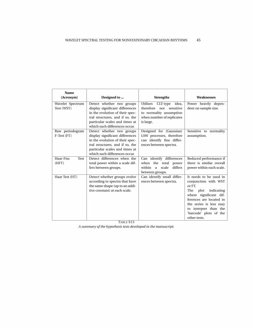
WAVELET SPECTRAL TESTING FOR NONSTATIONARY CIRCADIAN RHYTHMS 45
Name
(Acronym) Designed to ... Strengths Weaknesses
Wavelet Spectrum
Test (WST)
Detect whether two groups
display significant differences
in the evolution of their spec-
tral structures, and if so, the
particular scales and times at
which such differences occur.
Utilises CLT-type idea,
therefore not sensitive
to normality assumption
when number of replicates
is large.
Power heavily depen-
dent on sample size.
Raw periodogram
F-Test (FT)
Detect whether two groups
display significant differences
in the evolution of their spec-
tral structures, and if so, the
particular scales and times at
which such differences occur.
Designed for (Gaussian)
LSW processes, therefore
can identify fine differ-
ences between spectra.
Sensitive to normality
assumption.
Haar-Fisz Test
(HFT)
Detect differences when the
total power within a scale dif-
fers between groups.
Can identify differences
when the total power
within a scale differs
between groups.
Reduced performance if
there is similar overall
power within each scale.
Haar Test (HT) Detect whether groups evolve
according to spectra that have
the same shape (up to an addi-
tive constant) at each scale.
Can identify small differ-
ences between spectra.
It needs to be used in
conjunction with WST
or FT.
The plot indicating
where significant dif-
ferences are located in
the series is less easy
to interpret than the
‘barcode’ plots of the
other tests.
TABLE S15
A summary of the hypothesis tests developed in the manuscript.
46 J. K. HARGREAVES ET AL.
Bell-Pedersen, D., Cassone, V. M., Earnest, D. J., Golden, S. S., Hardin, P. E., Thomas, T. L., and Zo-
ran, M. J. (2005). Circadian rhythms from multiple oscillators: lessons from diverse organisms.
Nature Reviews Genetics, 6(7):544–556.
Benjamini, Y. and Hochberg, Y. (1995). Controlling the false discovery rate: a practical and power-
ful approach to multiple testing Journal of the royal statistical society. Series B (Methodological),
JSTOR, 57:289–300.
Bujdoso, N. and Davis, S. J. (2013). Mathematical modeling of an oscillating gene circuit to un-
ravel the circadian clock network of Arabidopsis thaliana. Frontiers in Plant Science, 4:3.
Cho, H. (2016). A test for second-order stationarity of time series based on unsystematic sub-
samples. Stat, 5(1): 262–277.
Costa, M. J., Finkenstädt, B., Gould, P. D., Foreman, J., Halliday, K. J., Hall, A. J. W and Rand,
D. A. (2011). Estimating periodicity of oscillatory time series through resampling techniques
University of Warwick. Centre for Research in Statistical Methodology.
Das, S. and Nason, G. P. (2016). Measuring the degree of non-stationarity of a time series. Stat,
5(1):295–305.
Doyle, M. R., Davis, S. J., Bastow, R. M., McWatters, H. G., Kozma-Bognár, L., and Nagy, Ferenc
and Millar, A. J. and Amasino, R. M. (2002). The ELF4 gene controls circadian rhythms and
flowering time in Arabidopsis thaliana. Nature, 419(6902): 74–77.
Dusik, V., Senthilan, P. R., Mentzel, B., Hartlieb, H., Wülbeck, C., Yoshii, T., Raabe, T. and Helfrich-
Förster, C. (2014). The MAP kinase p38 is part of Drosophila melanogaster’s circadian clock.
PLoS genetics, 10(8):e1004565.
Edwards, K. D., Akman, O. E., Knox, K., Lumsden, P. J., Thomson, A. W., Brown, P. E., Pokhilko, A.,
Kozma-Bognar, L., Nagy, F., Rand, D. A., and Millar, A. (2010). Quantitative analysis of regulatory
flexibility under changing environmental conditions. Molecular systems biology, 6(1): 424.
Fan, J. and Lin, S.-K. (1998). Test of significance when data are curves Journal of the American
Statistical Association, 93(443):1007–1021.
Foley, J. A.,DeFries, R., Asner, G. P., Barford, C., Bonan, G., Carpenter, S. R., Chapin, F S., Coe,
M. T., Daily, G. C., Gibbs, H. K. and others (2005). Global consequences of land use. Science,
American Association for the Advancement of Science, 309(5734):570–574.
Fryzlewicz, P. (2005). Modelling and forecasting financial log-returns as locally stationary wavelet
processes. Journal of Applied Statistics, 32(5):503–528.
Fryzlewicz, P. and Nason, G. P. (2006). Haar–fisz estimation of evolutionary wavelet spectra. Jour-
nal of the Royal Statistical Society: Series B (Statistical Methodology), 68(4):611–634.
Fryzlewicz, P. and Ombao, H. (2009). Consistent classification of nonstationary time series using
stochastic wavelet representations. Journal of the American Statistical Association, 104:299–
312.
Fryzlewicz, P., Van Bellegem, S. and von Sachs, R. (2003). Forecasting non-stationary time series
by wavelet process modelling. Annals of the Institute of Statistical Mathematics, 55(4):737–764.
Goya, M. E., Romanowski, A., Caldart, C. S., Bénard, C. Y. and Golombek, D. A. (2016). Circadian
rhythms identified in Caenorhabditis elegans by in vivo long-term monitoring of a biolumines-
cent reporter. Proceedings of the National Academy of Sciences, 201605769.
Guo, W., Dai, M., Ombao, H. C. and von Sachs, R.(2003). Smoothing spline ANOVA for time-
dependent spectral analysis. Journal of American Statistical Association, 98(463):643–652.
Hanano, S., Domagalska, M. A., Nagy, F., and Davis, S. J. (2006). Multiple phytohormones influence
distinct parameters of the plant circadian clock. Genes to Cells, 11(12):1381–1392.
Harang, R. Bonnet, G. and Petzold, L. R. (2006). WAVOS: a MATLAB toolkit for wavelet analysis
and visualization of oscillatory systems BMC research notes, BioMed Central, 5(1):163.
Hargreaves, J. K., Knight, M. I., Pitchford, J. W., Oakenfull, R. and Davis, S. J. (2018). Clustering
Nonstationary Circadian Rhythms using Locally Stationary Wavelet Representations. SIAM
Multiscale modeling and simulation, 16(1):184–214.

WAVELET SPECTRAL TESTING FOR NONSTATIONARY CIRCADIAN RHYTHMS 47
Hoagland, D. R. and Arnon, D. I. (1950). The water-culture method for growing plants without
soil. California Agricultural Experiment Station, Circular, 347.
Holan, S. H., Wikle, C. K., Sullivan-Beckers, L. E., and Cocroft, R. B. (2010). Modeling complex
phenotypes: generalized linear models using spectrogram predictors of animal communica-
tion signals. Biometrics, 66(3):914–924.
Killick, R., Eckley, I. A., and Jonathan, P. (2013). A wavelet-based approach for detecting changes
in second order structure within nonstationary time series. Electronic Journal of Statistics,
7:1167–1183.
Kon, N., Sugiyama, Y., Yoshitane, H., Kameshita, I. and Fukada, Y. (2015). Cell-based inhibitor
screening identifies multiple protein kinases important for circadian clock oscillations. Com-
municative & integrative biology, 8(4):e982405.
Krzemieniewska, K., Eckley, I. A., and Fearnhead, P. (2014). Classification of non-stationary time
series. Stat, 3(1):144–157.
Lagido, C., Pettitt, J., Flett, A. and Glover, L. A. (2008). Bridging the phenotypic gap: real-time as-
sessment of mitochondrial function and metabolism of the nematode Caenorhabditis elegans.
BMC physiology, 8(1):7.
Leise, T. L.,Indic, P., Paul, M. J. and Schwartz, W. J. (2013). Wavelet meets actogram. Journal of
biological rhythms, SAGE Publications Sage CA: Los Angeles, CA, 28(1):62–68.
Martinez J. G., Bohn K. M., Carroll R. J. and Morris J. S.(2013). A study of Mexican free-tailed bat
chirp syllables: Bayesian functional mixed modeling for nonstationary acoustic time series.
Journal of American Statistical Association, 108(502):514–526.
McClung, C. R. (2006). Plant circadian rhythms. The Plant Cell, 18(4):792–803.
McKay, J. L., Welch, T. D. J., Vidakovic, B. and Ting, L. H. (2012). Statistically significant con-
trasts between EMG waveforms revealed using wavelet-based functional ANOVA. Journal of
neurophysiology, 109(2):591–602.
Millar, A. J. and Carrington, J. T., Tee, W. V. and Hodge, S. K. (2015). Changing planetary rotation
rescues the biological clock mutant lhy cca1 of Arabidopsis thaliana. bioRxiv at Cold Spring
Harbor Laboratory.
Minors, D. S. and Waterhouse, J. M. (2013). Circadian rhythms and the human. Butterworth-
Heinemann
Moore, A., Zielinski, T., and Millar, A. J. (2014). Online period estimation and determination of
rhythmicity in circadian data, using the BioDare data infrastructure. Methods in Molecular
Biology, 1158:13–44.
Moore, D. S. (2007). The basic practice of statistics, (Vol. 2), WH Freeman, New York.
Morris, J. S. (2015). Functional regression. Annual Review of Statistics and Its Application, 2:321–
359.
Morris J. S., Baladandayuthapani V., Herrick R. C., Sanna P. and Gutstein H. (2011). Automated
analysis of quantitative image data using isomorphic functional mixed models, with applica-
tion to proteomics data. Annals of Applied Statistics, 5(2A):894–923.
Murashige, T. and Skoog, F. (1962). A revised medium for rapid growth and bio assays with tobacco
tissue cultures Physiologia plantarum, 15(3):473–497.
Nason, G. P. and Savchev, D. (2014). White noise testing using wavelets. Stat, 3(1):351–362.
Nason, G. P., Von Sachs, R., and Kroisandt, G. (2000). Wavelet processes and adaptive estimation of
the evolutionary wavelet spectrum. Journal of the Royal Statistical Society: Series B (Statistical
Methodology), 62(2):271–292.
Nason, G. (2010). Wavelet methods in Statistics with R. Springer Science & Business Media.
Nason, G. (2013). A test for second-order stationarity and approximate confidence intervals for
localized autocovariances for locally stationary time series. Journal of the Royal Statistical So-
ciety: Series B (Statistical Methodology), Wiley Online Library, 75(5):879–904.
Nason, G. P. and Stevens, K. (2015). Bayesian Wavelet Shrinkage of the Haar-Fisz Transformed

48 J. K. HARGREAVES ET AL.
Wavelet Periodogram. PloS one, Public Library of Science, 10(9):e0137662.
Nicholson, F. A., Smith, S. R., Alloway, B. J., Carlton-Smith, C. and Chambers, B. J. (2003). An
inventory of heavy metals inputs to agricultural soils in England and Wales. Science of the total
environment, Elsevier, 311(1):205–219.
Ogden, T. R. (1997). On preconditioning the data for the wavelet transform when the sample size
is not a power of two. Communications in Statistics-Simulation and Computation, 26(2):467–
486.
Oh, H.-S., Ammann, C. M., Naveau, P., Nychka, D., and Otto-Bliesner, B. L. (2003). Multi-resolution
time series analysis applied to solar irradiance and climate reconstructions. Journal of atmo-
spheric and solar-terrestrial physics, 65(2):191–201.
Perea-García, A., Andrés-Bordería, A., de Andrés, S. M., Sanz, A., Davis, A. M., Davis, S. J., Hui-
jser, P., and Peñarrubia, L. (2015). Modulation of copper deficiency responses by diurnal and
circadian rhythms in arabidopsis thaliana. Journal of experimental botany, 67(1):391–403.
Plautz, J. D., Straume, M., Stanewsky, R., Jamison, C. F., Brandes, C.,Dowse, H. B., Hall, J. C. and Kay,
S. A. (1997). Quantitative analysis of Drosophila period gene transcription in living animals.
Journal of Biological Rhythms, Sage Publications , 12(3): 204–217.
Price, T. S., Baggs, J. E., Curtis, A. M., FitzGerald, G. A. and Hogenesch, J. B. (2008). WAVECLOCK:
wavelet analysis of circadian oscillation Bioinformatics, Oxford University Press, 24(23): 2794–
2795.
Priestley, M. and Rao, T. S. (1969). A test for non-stationarity of time-series. Journal of the Royal
Statistical Society, Series B (Methodological), 31:140–149.
Priestley, M. B. (1982). Spectral analysis and time series. Academic Press.
Ramsay, J. O. and Silverman, B. W. (2005). Functional Data Analysis. Springer.
Von Sachs, R. and Neumann, Mi. H. (2000). A Wavelet-Based Test for Stationarity. Journal of Time
Series Analysis, Wiley Online Library, 21(5):597–613.
Senesil, G. S., Baldassarre, G., Senesi, N. and Radina, B. (1998). Trace element inputs into soils by
anthropogenic activities and implications for human health. Chemosphere, Elsevier, 39(2):343–
377.
Shumway, R. H. (1988). Applied Statistical Time Series Analysis. Statistics & probability letters,
63(3):307–314.
Southern, M. M. and Millar, A. J. (2005). Circadian genetics in the model higher plant, arabidopsis
thaliana. Methods in enzymology, 393:23–35.
Stiernagle, T. (1999). Maintenance of C. elegans. C. elegans: A Practical Approach, Oxford Univer-
sity Press, Oxford, UK, 2:51–67.
Tavakoli, S. and Panaretos, V. M. (2016). Detecting and localizing differences in functional time
series dynamics: a case study in molecular biophysics. Journal of the American Statistical As-
sociation, 111(515):1020–1035.
Torrence, C. and Compo, G. P. (1998). A practical guide to wavelet analysis. Bulletin of the Ameri-
can Meteorological society, 79(1):61–78.
Van Bellegem, S. and von Sachs, R. (2008). Locally adaptive estimation of evolutionary wavelet
spectra. Annals of Statistics, 36(4):1879–1924.
Vidakovic, B. (2001). Wavelet-based functional data analysis: theory, applications and ramifica-
tions. Proceedings of the 3rd Pacific Symposium on Flow Visualization and Image Processing,
Maui, HI.
Vitaterna, M. H., Takahashi, J. S., and Turek, F. W. (2001). Overview of circadian rhythms. Alcohol
Research and Health, 25(2):85–93.
Zielinski, T., Moore, A. M., Troup, E., Halliday, K. J. and Millar, A. J. (2014). Strengths and lim-
itations of period estimation methods for circadian data. PloS one, Public Library of Science,
9(5):96462.

WAVELET SPECTRAL TESTING FOR NONSTATIONARY CIRCADIAN RHYTHMS 49
DEPARTMENT OF MATHEMATICS
UNIVERSITY OF YORK
YORK
YO10 5DD, UK
E-MAIL: [email protected]
DEPARTMENTS OF MATHEMATICS AND BIOLOGY
UNIVERSITY OF YORK
YORK
YO10 5DD, UK
E-MAIL: [email protected]
DEPARTMENT OF BIOLOGY
UNIVERSITY OF YORK
YORK
YO10 5DD, UK
E-MAIL: [email protected]