Deterministic EOQ Models for Non-Linear Time ... - CORE

I S S N 2 3 4 7 - 1 9 2 1 V o l u m e 1 2 N u m b e r 2

J o u r n a l o f A d v a n c e s i n M a t h e m a t i c s

5949 | P a g e c o u n c i l f o r I n n o v a t i v e R e s e a r c h

A p r i l 2 0 1 6 w w w . c i r w o r l d . c o m

Deterministic EOQ Models for Non-Linear Time Induced Demand and Different Holding Cost Functions

R.P.Tripathi, *D.Singh and *Surbhi Aneja Department of mathematics, Graphic Era University, Dehradun (UK) India

[email protected] *Department of mathematics, SGRR (P. G) College, Dehradun (UK) India

[email protected] *Department of mathematics, SGRR (P. G) College, Dehradun (UK) India

[email protected]

ABSTRACT

This paper presents an Economic order quantity (EOQ) model for deteriorating items. The demand rate is non-linear function of time. In this paper two models have been derived for different holding costs (i). The holding cost is linear function of the on hand inventory level and (ii). A non-linear function of time for which the item is kept in the stock.

Optimization is done for both the models and numerical examples are presented to check the feasibility of the optimal solutions. Sensitivity analysis is also presented with respect to the various parameters used in the numerical example.

Indexing terms/Keywords

Deterioration; inventory; non-linear holding cost; EOQ Model

Academic Discipline And Sub-Disciplines

Mathematics (Operations Research)

SUBJECT CLASSIFICATION

90B05

TYPE (METHOD/APPROACH)

Theoretical approach

INTRODUCTION

Controlling and managing the inventory is among the biggest concern for any business regardless of its level. This concern leads the researchers to make inventory models for the better management of inventory. But while dealing with the real life problems it is not possible to consider all the factors affecting the depletion of inventory. Yet researchers have been able to consider most of the phenomenon like deterioration, demand rate etc.

As most of the physical goods undergo deterioration due to spoilage and many other factors. Most of the eatables that are available in market use preservatives. So they cannot be use after a definite time. So deterioration is an important factor to consider while developing an inventory model. Balkhi and Benkherouf (2004) developed an inventory model for deteriorating items with stock dependent and time varying demand rates. Lee and Dye (2012) established inventory model for deteriorating items under stock dependent demand rate and controllable deterioration rate. Arinadav and Herbon (2013) presented optimal inventory policy for a perishable item with demand function sensitive to price and time. Chang et al. (2010) presented optimal replenishment for non-instantaneous deteriorating items with stock-dependent demand. Giri and Chaudhari have developed many inventory models for the deteriorating items. Moon and Giri (2005) developed Economic order quantity models for ameliorating or deteriorating items under inflation and time discounting. Giri, Chaudhari and Goswami (1996) presented an inventory model for deteriorating items with stock-dependent demand rate. Giri and Chaudhari (1998) established deterministic model of perishable inventory with stock dependent demand rate and non-linear holding cost.

Most of the inventory models have been developed with constant holding cost. But this is not a realistic case. Weiss (1982) has taken no-linear holding cost in his paper. Goh (1994) also presented EOQ model with general demand and holding cost functions. Muhlemann and Valris (1980) have also taken variable holding cost rate in formulating the EOQ model. Singh, Tripathi and Mishra (2013) developed inventory model with deteriorating items and time-dependent holding cost. Tripathi and singh (2015) presented an inventory model with stock-dependent demand and different holding cost function. Other studies that have been done in this area can be marked for Alfares (2007), Pando (2013), Tripathi (2015) and Roy (2008).

In real life it is observed that the demand rate is often influenced by the amount of on-hand inventory. Soni and Shah(2008) presented a mathematical model to formulate optimal ordering policies for retailer when demand is partially constant and partially stock-dependent and the supplier offer progressive permissible delay to settle the account. Silver

brought to you by COREView metadata, citation and similar papers at core.ac.uk

provided by KHALSA PUBLICATIONS

https://core.ac.uk/display/322470781?utm_source=pdf&utm_medium=banner&utm_campaign=pdf-decoration-v1

mailto:[email protected]





and Peterson (1982) established an inventory model in which retail level is directly propotional to the amount of inventory displayed. Gupta and Vrat (1986) established EOQ model for demand rate is a function of initial stock level.

In this paper the main aim is to find optimal cycle time which minimizes the total relevant cost. The rest of the paper is organized as follows. Assumptions and notations are given in section 2 followed by mathematical formulation. Numerical examples are discussed in section 4. In section 5 we provide sensitivity analysis, Conclusions and future research directions have been marked in the last section 6.

2 ASSUMPTIONS AND NOTATIONS

Following assumptions are made throughout the manuscript

1. The demand is a function of power of time.

2. Shortages are not allowed.

3. The deterioration rate is constant i.e. 0 ˂ Ɵ ˂ 1.

4. The replenishment is instantaneous.

5. The lead time is negligible.

In addition the following notations are used in the whole manuscript-

q t - Inventory level at time t

1D t - Demand rate

1D - Scale parameter, 1 0D

- Shape parameter, 0 1

- Deterioration rate, 0 < < 1

h - Holding cost per unit item per unit time

HC - Holding cost during the cycle

DC – Deterioration cost per cycle

Q - Order quantity in one cycle

TCU - Total relevant inventory cost

K - The cost of placing an order

1C - Cost per unit item

3. MATHEMATICAL MODEL

At the initial level of cycle time T the inventory level is Q which is depleted during the cycle time T due to constant rate of deterioration and time dependent demand rate and becomes zero at the end of cycle time T.

The differential equation describing the changes in the inventory level q t over the period ( 0 t T ) is given by:

1 ;0

dq tq t D t t T

dt

, (1)

With the boundary condition 0q Q and 0q T .

Solving (1) and neglecting higher powers of we get

1 1 1 2

1

1 1 1

1 1 2 1 2

t Tq t D T t T t





2 2 21 32 1 2 1

2 1 2 3 2 2 3

t tT TT t

(2)

The order quantity for one cycle is

2 21

1

1 1

1 2 2 3

T TQ D T

(3)

3.1. Model A: In this model, the holding cost is taken to be the linear function of on- hand inventory level q t .

Therefore, the holding cost is

0

T

HC hq t dt (4)

Substituting (2) in (4) gives

1

0

( )

T

HC D h q t dt 2 2

2

1

1 1 1

2 2 3 6 4

T TD hT

(5)

The deterioration cost is given by

1 1

0

T

DC C Q D t dt

(6)

Using (3) in (6), we have

Deterioration cost is

2

1 1

1

2 2 3

TDC D C T

(7)

The total relevant cost per unit time is given by

K HC DCTCU

T

(8)

2 21 1

1 1 1

1 1

2 2 3 6 4 2 2 3

K T T TTCU D hT D C T

T

(9)

In this paper our main concern is to find the optimal order quantity Q, which minimizes the total relevant cost TCU of the

inventory model.

The necessary condition for the TCU to be minimum is

0d

TCUdT

Which give

d d

T HC DC K HC DCdT dT

(10)

Substituting the value of HC and DC from equation (5) and (7), the above equation reduces to





2 2 32

2

1

1

1

1 1

11

2 2 6 2 3 6 4

11

2 2 2 3

D hT

D C T K

TT T

TT

(11)

From the above expression we can calculate the value of T , that can be used to calculate the value of Q

by

substituting in (3), which minimizes the total relevant cost TCU of the inventory system, provided 2

20

d TCU

dT .

The second derivative of (9) w.r.t T is given by

2

1

1 1 1 12 3

21

1

1 1 22

2 2 3

2 3

6 4

d TCU KD h C T D h C T

dT T

D h T

(12)

It can be seen from (12) that 2

20

d TCU

dT , which shows that TCU gives minimum value at T=T

*(T=T

* obtained on

solving (11) for T)

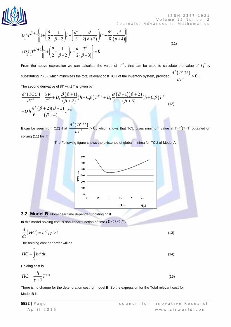
The Following figure shows the existence of global minima for TCU of Model A.

3.2. Model B: Non-linear time dependent holding cost

In this model holding cost is non-linear function of time ( 0 t T ).

; 1d

HC htdt

(13)

The holding cost per order will be

0

T

HC ht dt (14)

Holding cost is

1

1

hHC T

(15)

There is no change for the deterioration cost for model B, So the expression for the Total relevant cost for

Model B is





1 2 2

1 1 1 11 2 2 3

K h T TTCU T D C D C

T

(16)

Differentiating (14) w.r.to cycle time T and equating it to zero, we will get the expression

21

1 1

11 1

1 2 2 2 3

T ThT D C T T K

(17)

Differentiating (14) w.r.to cycle time T, twice yields

2 2

1

1 12 3

2

1 1

1 12

1 2

1 2

2 3

d TCU h TKD C T

dT T

D C T

(18)

By putting various values of the parameters, we will be able to find the value of T and Q

(Optimal value of T and Q)

numerically. To minimize the Total relevant cost TCU, cycle time T and order quantity Q, the following condition should be

satisfied − 2

20

d TCU

dT

.

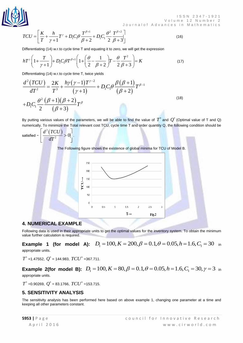
The Following figure shows the existence of global minima for TCU of Model B.

4. NUMERICAL EXAMPLE

Following data is used in their appropriate units to get the optimal values for the inventory system. To obtain the minimum value further calculation is required.

Example 1 (for model A): 1 1100, 200, 0.1, 0.05, 1.6, 30D K h C in

appropriate units.

T =1.47552, Q

= 144.983, TCU =367.711.

Example 2(for model B): 1 1100, 80, 0.1, 0.05, 1.6, 30, 3D K h C in

appropriate units.

T =0.90269, Q

= 83.1766, TCU =153.715.

5. SENSITIVITY ANALYSIS

The sensitivity analysis has been performed here based on above example 1, changing one parameter at a time and keeping all other parameters constant.





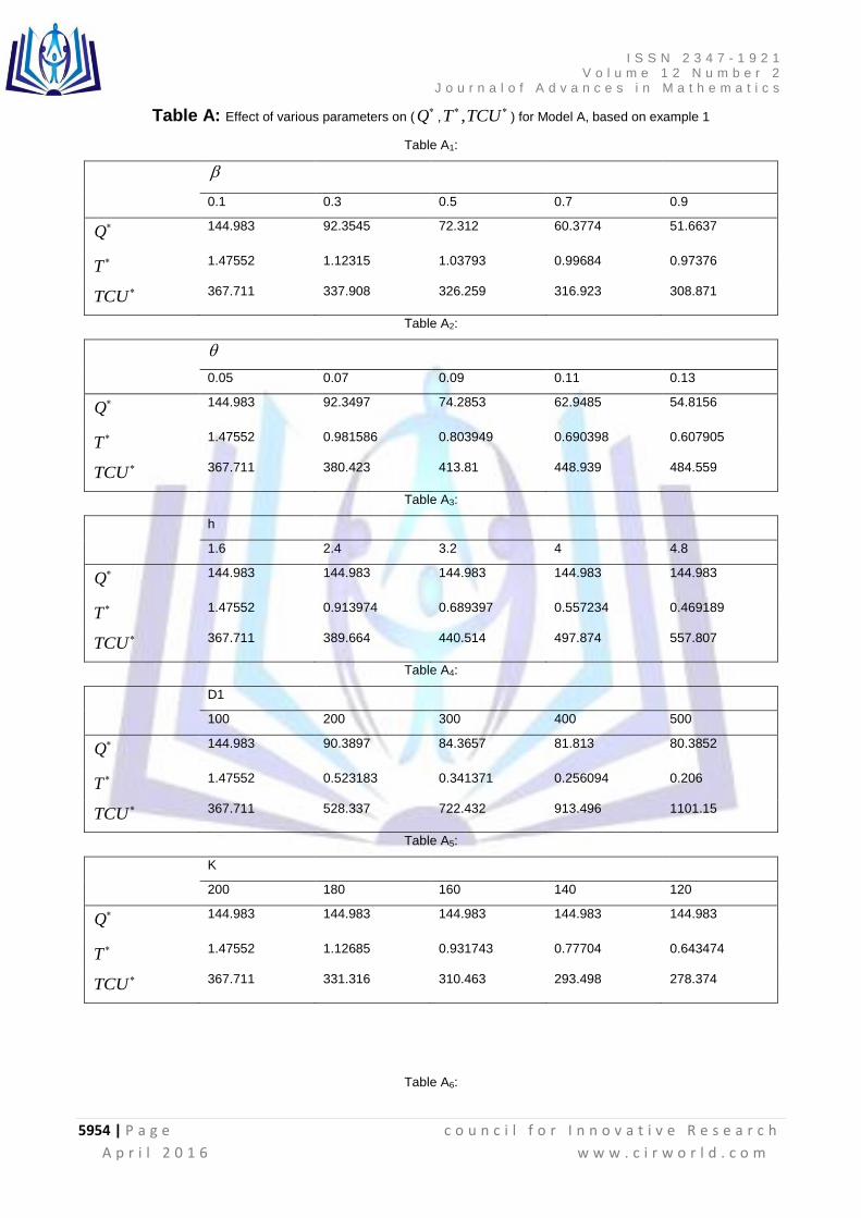
Table A: Effect of various parameters on ( Q, ,T TCU

) for Model A, based on example 1

Table A1:

0.1 0.3 0.5 0.7 0.9

Q

144.983 92.3545 72.312 60.3774 51.6637

T

1.47552 1.12315 1.03793 0.99684 0.97376

TCU

367.711 337.908 326.259 316.923 308.871

Table A2:

0.05 0.07 0.09 0.11 0.13

Q

144.983 92.3497 74.2853 62.9485 54.8156

T

1.47552 0.981586 0.803949 0.690398 0.607905

TCU

367.711 380.423 413.81 448.939 484.559

Table A3:

h

1.6 2.4 3.2 4 4.8

Q

144.983 144.983 144.983 144.983 144.983

T

1.47552 0.913974 0.689397 0.557234 0.469189

TCU

367.711 389.664 440.514 497.874 557.807

Table A4:

D1

100 200 300 400 500

Q

144.983 90.3897 84.3657 81.813 80.3852

T

1.47552 0.523183 0.341371 0.256094 0.206

TCU

367.711 528.337 722.432 913.496 1101.15

Table A5:

K

200 180 160 140 120

Q

144.983 144.983 144.983 144.983 144.983

T

1.47552 1.12685 0.931743 0.77704 0.643474

TCU

367.711 331.316 310.463 293.498 278.374

Table A6:





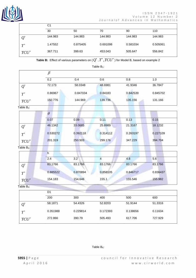
C1

30 50 70 90 110

Q

144.983 144.983 144.983 144.983 144.983

T

1.47552 0.875405 0.691098 0.581034 0.505061

TCU

367.711 399.63 453.043 505.647 556.842

Table B: Effect of various parameters on ( Q, ,T TCU

) for Model B, based on example 2

Table B1:

0.2 0.4 0.6 0.8 1.0

Q

72.173 58.0348 48.6981 41.9346 36.7847

T

0.86967 0.847034 0.84183 0.842539 0.845702

TCU

150.776 144.969 139.736 135.156 131.166

Table B2:

0.07 0.09 0.11 0.13 0.15

Q

46.1342 33.0685 25.8989 21.3167 18.1232

T

0.530272 0.392118 0.314112 0.263197 0.227109

TCU

201.319 250.503 299.176 347.229 394.704

Table B3:

h

2.4 3.2 4 4.8 5.6

Q

83.1766 83.1766 83.1766 83.1766 83.1766

T

0.885522 0.870894 0.858105 0.846717 0.836437

TCU

154.183 154.646 155.1 155.546 155.982

Table B4:

D1

200 300 400 500 600

Q

58.1871 54.4326 52.8203 51.9144 51.3316

T

0.351988 0.229814 0.172393 0.138656 0.11634

TCU

272.866 390.79 505.493 617.706 727.929

Table B5:





K

70 60 50 40 30

Q

83.1766 83.1766 83.1766 83.1766 83.1766

T

0.706808 0.567926 0.452919 0.35162 0.259128

TCU

148.526 144.424 140.549 136.534 132.022

Table B6:

C1

50 70 90 110 130

Q

83.1766 83.1766 83.1766 83.1766 83.1766

T

0.432361 0.29815 0.22981 0.187881 0.159369

TCU

232.741 312.582 390.79 467.567 543.144

The results of table A can be summed up as follows-

(i). From the table A1 it is relevant that as the value of scale parameter β increases optimal order quantity Q* decreases

and so the optimal cycle time T* and Total relevant cost TCU

*.

(ii). From table A2 it is clear that the increasing effect of deterioration rate increases TCU* but decreases Q* and T

*.

(iii). Table A3 shows the variation in the value of Q*, T

* and TCU

* with respect to the per unit holding cost h. There is no

change in optimal order quantity corresponding to unit holding cost h. Whereas increment in the value of h decreases the optimal cycle time T* and increase in the total relevant cost TCU

*.

(iv). Table A4 indicates that the increment in the scale parameter D1 results the decrement Q* and T* but increment in

TCU*.

(v). From Table A5, we see that a significant decrease in the unit ordering cost K leaves no change in Q* but produces a

significant decrease in T* and TCU*.

(vi). Table A6 shows that as the value of per unit item cost C1 increases, TCU* increases and T

* decreases, whereas no

change is seen in Q*.

The results of Table B summarized in the following points:

(i). Increase of shape parameter β causes significant decrease in Q* and TCU

*.But there is insignificant change in T

*with

respect to increase in β.

(ii). Increase of unit holding cost h cause insignificant changes in T* and TCU

* change for Q

*.So the change of h will cause

insignificant change in T*, Q

* and TCU

*.

(iii). Increase of Ɵ causes significant increase in TCU*, decrease in T

* and Q

*.So the positive change in Ɵ will lead positive

change in TCU*and negative change in T

* and Q

*.

(iv). Positive change in scale parameter D1 and C1 causes significant positive change in TCU* and negative change in T

*

but increase in D1 causes decrease in Q* whereas increase in C1 does not alter the Q

*.

6. CONCLUSION AND FUTURE RESEARCH

In this paper, we have developed inventory models with non-linear time dependent demand. Holding cost rate is taken as quantity dependent for model A and non-linear time-dependent for model B. This type of assumption is valid with time retailers which sells products like green vegetables, breads and seasonal fruits, whose quality decreases with time due to direct spoilage or physical decay. The time-dependent holding cost is realistic assumption because to arrange greater storage facilities to cease spoilage and to keep the freshness of the commodities in the stock cannot let the holding cost constant.

Mathematical models have been developed for two different situations. Sensitivity analysis with respect to variation of different parameters revealed significant changes in T

*, Q

* and TCU

*.

From managerial point of view, we can conclude the sensitivity of the parameters for T*, Q

* and TCU

* in the following

table-





For model A:

(1). Positive change of Ɵ and D1 results in positive change in TCU* but yields negative change in T

*and Q

*.

(2). Change in h and C1 leads positive change in TCU*, negative change in T

* and insignificant change in Q

*.

(3). Change in β result negative change in T*, Q

* and TCU

*.

(4). Negative change in K leads negative change in T*, TCU

* and leads no change in Q

*.

For model B:

(1). Positive change of Ɵ and D1 results in positive change in TCU* but yields negative change in T

*and Q

*.

(2). Change in h and C1 leads positive change in TCU*, negative change in T

* and insignificant change in Q

*.

(3). Change in β result negative change in T*and TCU

*, positive change in Q

*.

(4). Negative change in K leads negative change in T*, TCU

* and leads no change in Q

*.

The model discussed in this paper may be generalized to allow for shortages. We may also extend the present model for exponential demand as well as inflation dependent demand.

ACKNOWLEDGMENTS

The authors acknowledge the Editor-in-Chief of the journal and the anonymous reviewers for their indispensable input that improved the paper significantly. Our thanks to the experts who have contributed towards development of the template.

REFERENCES

1. A.P., Muhlemann, N.P., Valris, Sapanopoulos. “A variable holding cost rate EOQ model”, European Journal of Operational Research, 1980, 4, 132-135.

2. H.K. Alfares, “Inventory model with stock-level dependent demand rate and variable holding cost”, International Journal of Production Economics,2007, 108(1-2), 259-265.

3. T. Arinadav, A. Herbon, U. Spiegel, “Optimal inventory policy for a perishable item with demand function sensitive to price and time”, International Journal of Production Economics, 2013, 144(2), 497-506.

4. B. Vander Veen. 1967.Introduction to the theory of operational research. Philips Technical Library, Springer-Verlag, Newyork.

5. Z.P. Balkhi, L. Benkherouf, “On an inventory model for deterioration items with stock dependent and time-varying demand rates”, Computer and Operations Research, 2004, 31, 223-240.

6. C.T. Chang, J.T. Teng, S.K. Goyal, “Optimal replenishment policies for non-instantaneous deteriorating items with stock dependent demand”, International Journal of Production Economics, 2010, 123(1), 62-68.

7. C.Y. Dye, L.Y. Ouyang, “An EOQ model for perishable items under stock dependent selling rate and time-dependent partial backlogging”, European Journal of Operation Research, 2005, 163(3), 776-783.

8. E., Naddol. 1965.Inventory systems. Wiley, Newyork.

9. B.C. Giri and K.S. Chaudhari, “Deterministic model of perishable inventory with stock-dependent demand rate and non-linear holding cost”, European Journal of Operational Research, 1998, 105, 467-474.

10. B.C. Giri, S. Pal, A. Goswami, K.S. Chaudhari, “An inventory model for deteriorating items with stock-dependent demand rate”, European Journal of Operational Research,1996, 95(3), 604-610.

11. M. Goh, “EOQ models with general demand and holding cost functions”, European Journal of Operational Research, 1994, 73, 50-54.

12. R. Gupta, and P. Vrat, “Inventory model for stock-dependent consumption rate”,Opsearch, 1986, 23, 19-24.

13. Y.P. Lee, C.Y. Dye, “An inventory model for deteriorating items under stock-dependent demand rate and controllable deterioration rate”, Computer Ind. Engineering, 2012, 63(2), 474-482.

14. B.N. Mandal, S. Phaujdar, “An inventory model for deteriorating items and stock-dependent consumption rate”, Journal of Operation Research Society, 1989, 40(5), 483-488.

15. L. Moon, B.C. Giri and B. Ko, “Economic order quantity models for ameliorating or deteriorating items under inflation and time discounting”, European Journal of Operational Research, 2005, 162, 773-785.

16. S. Nahmtas, “Perishable inventory Theory: A Review”, Operations Research, 30(4), 680-708.





17. V. Pando, L.A. Sanjose, J. Garcia-Laguna, J. Sicillia, “An economic lot-size model with non-linear holding cost hinging on time and quantity”, International Journal of Production Economics, 2013, 145(1), 294-303.

A. Roy, “An inventory model for deteriorating items with price dependent demand and time-varying holding cost”, Advanced Modeling and Optimization, 2008,10(1), 25-36.

18. Silver, E.A., Peterson, R. 1985. Decision systems for inventory management and production planning; 2nd

Edition Wiley, New York.

19. D. Singh, R.P. Tripathi and T. Mishra, “Inventory model with deteriorating items and time dependent holding cost”, Global Journal of Mathematical Sciences Theory and Practical,2013, 5(4), 213-220.

20. H. Soni, and N.H. Shah, “Optimal ordering policy for stock dependent demand under progressive payment scheme”, European Journal of Operational Research, 2008,184, 91-100.

21. A.A. Taleizadeh, B. Mohammadi, L.E. Cardenas-Barron, H. Samimi, “An EOQ model for perishable product with special sale and shortage”, International Journal of Production Economics, 2013, 145(1), 318-338.

22. R.P. Tripathi, “Inventory model with different demand rate and different holding cost”, International J. Ind. Eng. Computation,2013, 4(3), 437-446.

23. R.P. Tripathi, D. Singh and T. Mishra, “Economic order quantity”, Journal of Mathematics and Statistics, 2015,11(1), 21-28.

24. R.P. Tripathi, D. Singh, “Inventory model with stock-dependent demand and different holding cost function”, International Journal of Industrial and System Engineering, 2015, 21(1), 68-72.

25. R.P. Tripathi, “Economic order quantity for deteriorating items with non-decreasing demand and shortages under inflation and time-discounting”, International Journal of Engineering, 2015, 28(9), 1058-1066.

26. R.P. Tripathi and M. Kumar, “A new model for deteriorating items with inflation under permissible delay in payment”, International Journal of Industrial Engineering Computation, 2014, 5, 365-374.

27. H.J. Weiss, “Economic order quantity models with non-linear holding cost”, European Journal of Operational Research, 1982, 9, 56-60.

28. K.S. Wu, L.Y. Ouyang, C.T. Yang, “An optimal replenishment policy for non-instantaneous deteriorating items with stock-dependent demand and partial backlogging”, International Journal of Production Economics, 2006,101(2), 369-384.

29. S.P. You, “Inventory policy for products with price and time-dependent demands”, Journal of the Operational Research Society,2005, 56, 870-873.

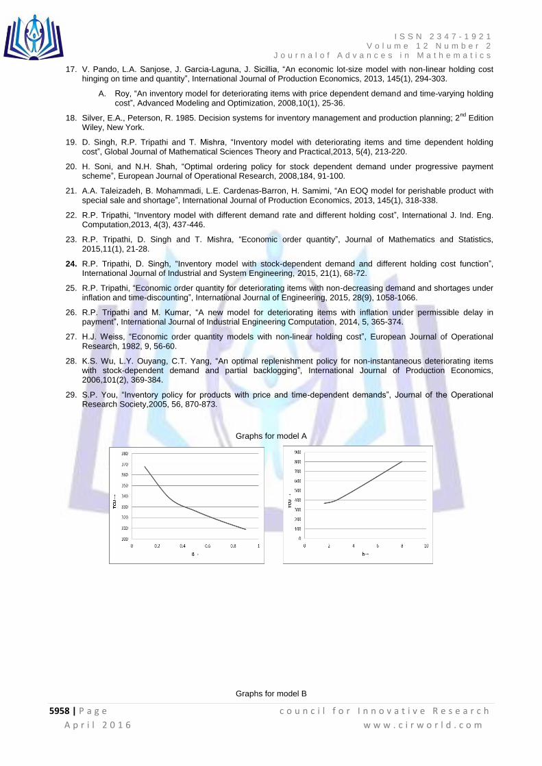
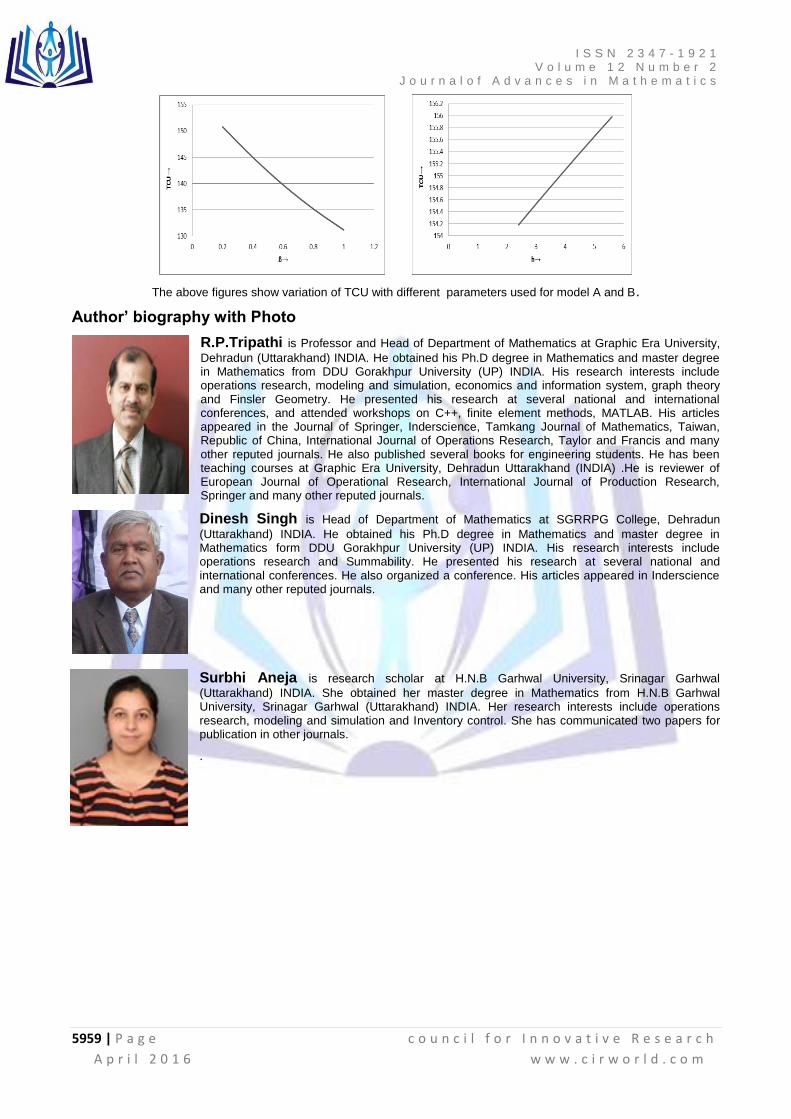
Graphs for model A

Graphs for model B





The above figures show variation of TCU with different parameters used for model A and B.

Author’ biography with Photo

R.P.Tripathi is Professor and Head of Department of Mathematics at Graphic Era University,

Dehradun (Uttarakhand) INDIA. He obtained his Ph.D degree in Mathematics and master degree in Mathematics from DDU Gorakhpur University (UP) INDIA. His research interests include operations research, modeling and simulation, economics and information system, graph theory and Finsler Geometry. He presented his research at several national and international conferences, and attended workshops on C++, finite element methods, MATLAB. His articles appeared in the Journal of Springer, Inderscience, Tamkang Journal of Mathematics, Taiwan, Republic of China, International Journal of Operations Research, Taylor and Francis and many other reputed journals. He also published several books for engineering students. He has been teaching courses at Graphic Era University, Dehradun Uttarakhand (INDIA) .He is reviewer of European Journal of Operational Research, International Journal of Production Research, Springer and many other reputed journals.

Dinesh Singh is Head of Department of Mathematics at SGRRPG College, Dehradun

(Uttarakhand) INDIA. He obtained his Ph.D degree in Mathematics and master degree in Mathematics form DDU Gorakhpur University (UP) INDIA. His research interests include operations research and Summability. He presented his research at several national and international conferences. He also organized a conference. His articles appeared in Inderscience and many other reputed journals.

Surbhi Aneja is research scholar at H.N.B Garhwal University, Srinagar Garhwal

(Uttarakhand) INDIA. She obtained her master degree in Mathematics from H.N.B Garhwal University, Srinagar Garhwal (Uttarakhand) INDIA. Her research interests include operations research, modeling and simulation and Inventory control. She has communicated two papers for publication in other journals.

.

Deterministic EOQ Models for Non-Linear Time ... - CORE

Documents

Transcript of Deterministic EOQ Models for Non-Linear Time ... - CORE