
On the Efficiency of Designs for Linear Models in Non-regular Regions and the Use of Standard...
122
On the Efficiency of Designs for Linear Models in Non-regular Regions and the Use of Standard Designs for Generalized Linear Models Alyaa R. Zahran Dissertation submitted to the Virginia Polytechnic Institute and State University in partial fulfillment of the requirements for the degree of Doctor of Philosophy in Statistics Christine Anderson-Cook, co-chair Raymond H. Myers, co-chair Eric P. Smith, co-chair John Morgan Keying Ye July 1, 2002 Blacksburg, Virginia Key Words: design optimality, fraction of design space technique, non-regular design spaces, linear models, generalized linear models
Transcript of On the Efficiency of Designs for Linear Models in Non-regular Regions and the Use of Standard...
On the Efficiency of Designs for Linear Models in Non-regular Regions
and the Use of Standard Designs for Generalized Linear Models
Alyaa R. Zahran
Dissertation submitted to the Virginia Polytechnic Institute and State University in partial
fulfillment of the requirements for the degree of
Doctor of Philosophy
in
Statistics
Christine Anderson-Cook, co-chair
Raymond H. Myers, co-chair
Eric P. Smith, co-chair
John Morgan
Keying Ye
July 1, 2002
Blacksburg, Virginia
Key Words: design optimality, fraction of design space technique, non-regular design
spaces, linear models, generalized linear models
On the Efficiency of Designs for Linear Models in Non-regular Regions
and the Use of Standard Designs for Generalized Linear Models
Alyaa R. Zahran
(ABSTRACT)
The Design of an experiment involves selection of levels of one or more factor in
order to optimize one or more criteria such as prediction variance or parameter variance
criteria. Good experimental designs will have several desirable properties. Typically, one
can not achieve all the ideal properties in a single design. Therefore, there are frequently
several good designs and choosing among them involves tradeoffs.
This dissertation contains three different components centered around the area of
optimal design: developing a new graphical evaluation technique, discussing designs for
non-regular regions for first order models with interaction for the two- and three-factor
case, and using the standard designs in the case of generalized linear models (GLM).
The Fraction of Design Space (FDS) technique is proposed as a new graphical
evaluation technique that addresses good prediction. The new technique is comprised of
two tools that give the researcher more detailed information by quantifying the fraction of
design space where the scaled predicted variance is less than or equal to any pre-specified
value. The FDS technique complements Variance Dispersion Graphs (VDGs) to give the
researcher more insight about the design prediction capability. Several standard designs
are studied with both methods: VDG and FDS.
Many Standard designs are constructed for a factor space that is either a p-
dimensional hypercube or hypersphere and any point inside or on the boundary of the

1
shape is a candidate design point. However, some economic, or practical constraints may
occur that restrict factor settings and result in an irregular experimental region. For the
two- and three-factor case with one corner of the cuboidal design space excluded, three
sensible alternative designs are proposed and compared. Properties of these designs and
relative tradeoffs are discussed.
Optimum experimental designs for GLM depend on the values of the unknown
parameters. Several solutions to the dependency of the parameters of the optimality
function were suggested in the literature. However, they are often unrealistic in practice.
The behavior of the factorial designs, the well-known standard designs of the linear case,
is studied for the GLM case. Conditions under which these designs have high G-
efficiency are formulated.

iv
Dedication
To my parents,
and to my husband, Farouk

v
AcknowledgementsAll praise and thanks is to Allah, the one, the only and the indivisible creator and
sustainer of the worlds. To Him, we belong and to Him, we will return. I wish to thank
Him for all that He has gifted me with, although, He can never be praised or thanked
enough.
I would like to express my deepest thanks and sincere appreciation to my
advisors: Prof. C. Anderson-Cook, Prof. R. Myers, and Prof. EP. Smith, for their strong
support throughout this study. Their high standards and goals, as well as their genuine
interest in science were both very challenging and motivating. I would like to thank Prof.
C. Anderson-Cook for her constant guidance, patience and encouragement. Grateful
acknowledgements to Prof. R. Myers for his enthusiasm, understanding, guidance and
considerable help throughout this research. I am truly thankful for Prof. E.P. Smith for
his valuable advice and assistance during this research.
I would like to express my appreciation to my committee members Prof. Morgan
and Prof. Ye for their valuable suggestions and interest during my research. Special
thanks to Prof. G. Terrell for his valuable comments in this research.
I am grateful to the Virginia Water Resources Research Center and U.S.
Environmental Protection Agency’s Science to Achieve Results (STAR) for funding this project
(Grant No. R82795301).
Finally, I would like to give my special recognition to my husband, Farouk, for
his understanding, interest and support at every stage of this research. My deepest thanks
go to my parents for their love, prayer, support, and subtle encouragement throughout
my life.
vi
Table of Contents
List of Figures ______________________________________________ ix
List of Tables _______________________________________________ xi
Chapter I Introduction and Literature Review______________________1I.1 Introduction _______________________________________________ 1
I.2 Brief Review of Some Concepts in Optimality Theory_____________ 6I.2.1 Optimality Criteria and Efficiency__________________________________ 6
I.2.1.1 D-Optimality___________________________________________________________ 6I.2.1.2 G- Optimality __________________________________________________________ 7I.2.1.3 Q-Optimality___________________________________________________________ 7
I.2.2 The General Equivalence Theorem for D- and G-optimum designs ________ 8I.2.3 Orthogonality and Rotatability_____________________________________ 8
I.2.3.1 Orthogonality __________________________________________________________ 8I.2.3.2 Rotatability ____________________________________________________________ 9
I.2.4 Graphical Methods for the Performance of the Prediction Capability in theRegion of Interest____________________________________________________ 9
I.3 Some Response Surface Designs ______________________________ 10I.3.1 Two-Level Factorial and Fractional of Resolution III, IV _______________ 10I.3.2 Second Order Model Designs ____________________________________ 11
I.3.2.1 Central Composite Designs (CCD)_________________________________________ 11I.3.2.2 Box-Behnken Designs (BBD)_____________________________________________ 12I.3.2.3 Small Central Composite Designs (SCD)____________________________________ 12I.3.2.4 Hybrid Designs ________________________________________________________ 13
I.4 Design Optimality for Generalized Linear Models_______________ 13I.4.1 Locally Optimal Designs ________________________________________ 14I.4.2 Minimax Approach ____________________________________________ 14I.4.3 Bayesian Approach ____________________________________________ 15I.4.4 Sequential Designs Approach ____________________________________ 15
I.5 Layout of Dissertation ______________________________________ 15
I.6 References ________________________________________________ 16
Chapter II Fraction of Design Space to Assess the Prediction Capability of
Response Surface Designs ___________________________21II.1 Abstract __________________________________________________ 21
II.2 Introduction ______________________________________________ 21
II.3 Review of Variance Dispersion Graphs (VDG)__________________ 25
II.4 The Fraction of Design Space Criterion (FDS) __________________ 26
II.5 Comparisons of the Standard Second-Order Designs over Spherical
Region __________________________________________________ 29
vii
II.5.1 Example: Two Factors on Spherical Region _______________________ 30II.5.2 Example: Three Factors on Spherical Region ______________________ 30II.5.3 Example: Four Factors on Spherical Region _______________________ 34II.5.4 Example: Five Factors on Spherical Region________________________ 34II.5.5 Example: Six Factors on Spherical Region ________________________ 39
II.6 Comparisons of the Standard Second-Order Models over Cuboidal
Region with Three Factors __________________________________ 41
II.7 Conclusions _______________________________________________ 43
II.8 References ________________________________________________ 43
Chapter III Modifying 22 Factorial Designs to Accommodate a Restricted
Design Space _____________________________________45III.1 Abstract __________________________________________________ 45
III.2 Introduction ______________________________________________ 46
III.3 Design Space and Possible Designs____________________________ 47III.3.1 Design I____________________________________________________ 48III.3.2 Design II ___________________________________________________ 48III.3.3 Design III __________________________________________________ 49III.3.4 Comparison of Designs________________________________________ 49
III.4 Example__________________________________________________ 55
III.5 General Design Space and Design I ___________________________ 56
III.6 Conclusions and Discussion__________________________________ 58
III.7 References ________________________________________________ 59
Supplement I: Modifying 23 Factorial to Accommodate a Restricted Design
Space ____________________________________________ 61
Supplement II: FDS Technique for the Three Designs in Restricted Design
Space ____________________________________________ 71SII.1 Two-Factor Case ______________________________________________ 71SII.2 Three-Factor Case _____________________________________________ 76
Chapter IV Use of Standard Factorial Designs with Generalized Linear
Models_________________________________________80IV.1 Abstract __________________________________________________ 80
IV.2 Introduction ______________________________________________ 80
IV.3 Implementation of Standard Designs__________________________ 82
IV.4 Characteristics of the Information Matrix in GLM ______________ 83
viii
IV.4.1 Use of the two-level Factorial___________________________________ 84IV.4.2 Examples___________________________________________________ 85
IV.5 General Results for GLM with Canonical Link and Standard 22
Factorial Design ___________________________________________ 89IV.5.1 Properties of the Scaled Prediction Variance for the 22 Factorial Design _ 89IV.5.2 Interaction Model - Equal Asymptotic Variances of the Parameters Estimates
____________________________________________________________91IV.5.3 Interaction Model -the Scaled Prediction Variance at the Design Points__ 91
IV.6 A characterization of Efficiency for the Use of 22 Factorial Designswith the Logistic and Poisson Regression Models ____________________ 91
IV.6.1 First Order Models with and without Interaction: Logistic Regression ___ 91IV.6.2 First Order Models with and without Interaction: Poisson Regression ___ 93
IV.7 Variance Stabilizing Link ___________________________________ 94
IV.8 Real Life Example _________________________________________ 95
IV.9 Conclusions _______________________________________________ 96
IV.10 References ______________________________________________ 97
Appendix A: __________________________________________________ 100
Appendix B___________________________________________________ 102
Appendix C___________________________________________________ 104
Appendix D___________________________________________________ 106
Chapter V Summary and Future Work_________________________107
ix
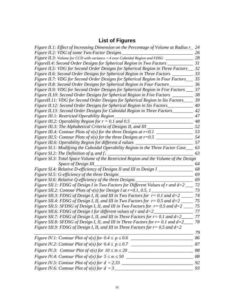
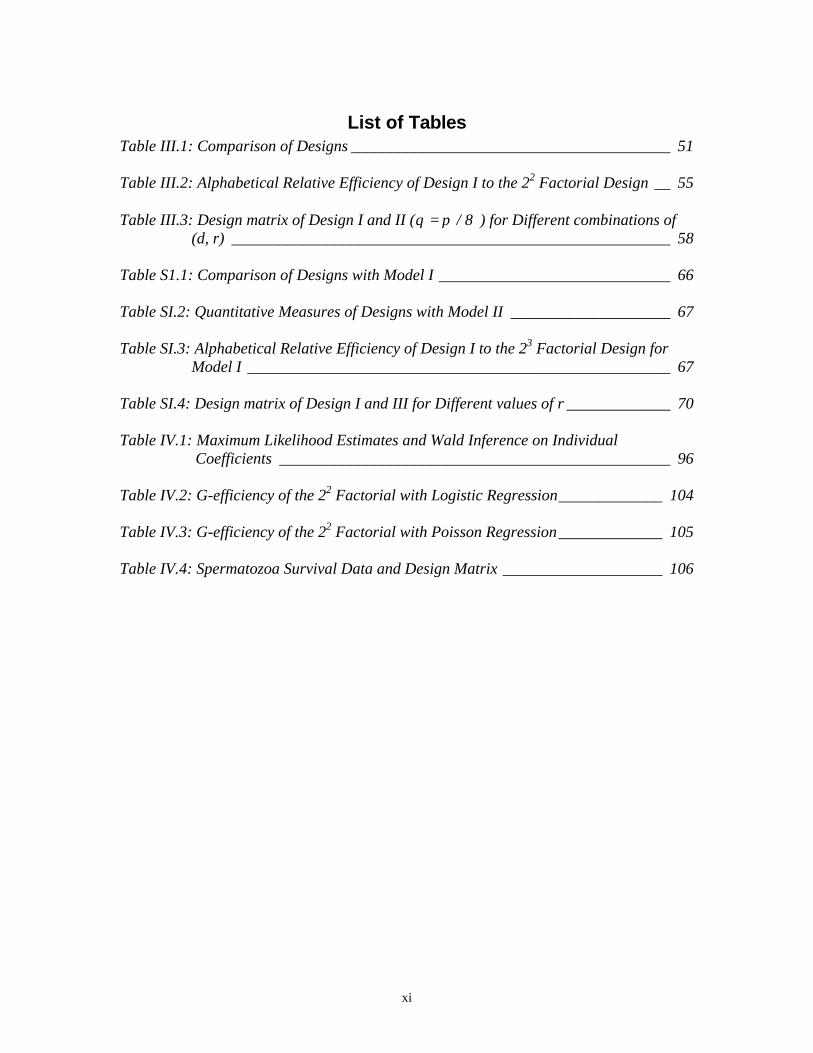
List of FiguresFigure II.1: Effect of Increasing Dimension on the Percentage of Volume at Radius r_ 24Figure II.2: VDG of some Two-Factor Designs _______________________________ 26Figure II.3: Volume for CCD with variance = 4 over Cuboidal Region and FDSG ____________ 28FigureII.4: Second Order Designs for Spherical Region in Two Factors ___________ 31Figure II.5: VDG for Second Order Designs for Spherical Region in Three Factors __ 32Figure II.6: Second Order Designs for Spherical Region in Three Factors _________ 33Figure II.7: VDG for Second Order Designs for Spherical Region in Four Factors___ 35Figure II.8: Second Order Designs for Spherical Region in Four Factors __________ 36Figure II.9: VDG for Second Order Designs for Spherical Region in Five Factors ___ 37Figure II.10: Second Order Designs for Spherical Region in Five Factors _________ 38FigureII.11: VDG for Second Order Designs for Spherical Region in Six Factors____ 39Figure II.12: Second Order Designs for Spherical Region in Six Factors___________ 40Figure II.13: Second Order Designs for Cuboidal Region in Three Factors_________ 42Figure III.1: Restricted Operability Region __________________________________ 47Figure III.2: Operability Region for r = 0.1 and 0.5 ___________________________ 48Figure III.3: The Alphabetical Criteria of Designs II, and III ____________________ 52Figure III.4: Contour Plots of v(x) for the three Designs at r=0.1 ________________ 53Figure III.5: Contour Plots of v(x) for the three Designs at r=0.5 ________________ 54Figure III.6: Operability Region for different d values _________________________ 57Figure SI.1: Modifying the Cuboidal Operability Region in the Three Factor Case___ 63Figure SI.2: The Definition of θi and φi _____________________________________ 63Figure SI.3: Total Space Volume of the Restricted Region and the Volume of the Design Space of Design III___________________________________________ 64Figure SI.4: Relative D-efficiency of Designs II and III to Design I _______________ 68Figure SI.5: G-efficiency of the three Designs ________________________________ 69Figure SI.6: Relative Q-efficiency of the three Designs _________________________ 69Figure SII.1: FDSG of Design I in Two Factors for Different Values of r and d=2 ___ 72Figure SII.2: Contour Plots of v(x) for Design I at r=0.1, 0.5, 1 __________________ 73Figure SII.3: FDSG of Design I, II, and III in Two Factors for r= 0.1 and d=2 _____ 74Figure SII.4: FDSG of Design I, II, and III in Two Factors for r= 0.5 and d=2 _____ 75Figure SII.5: SFDSG of Design I, II, and III in Two Factors for r= 0.5 and d=2 ____ 75Figure SII.6: FDSG of Design I for different values of r and d=2_________________ 77Figure SII.7: FDSG of Design I, II, and III in Three Factors for r= 0.1 and d=2_____ 77Figure SII.8: SFDSG of Design I, II, and III in Three Factors for r= 0.1 and d=2____ 78Figure SII.9: FDSG of Design I, II, and III in Three Factors for r= 0.5 and d=2_____________________________________________________________________ 79Figure IV.1: Contour Plot of v(x) for 6.0p4.0 ≤≤ ___________________________ 86Figure IV.2: Contour Plot of v(x) for 7.0p4.0 ≤≤ ___________________________ 87Figure IV.3: Contour Plot of v(x) for 2010 ≤≤ µ ____________________________ 88Figure IV.4: Contour Plot of v(x) for 505 ≤≤ µ _____________________________ 88Figure IV.5: Contour Plot of v(x) for 33.2=δ _______________________________ 92Figure IV.6: Contour Plot of v(x) for 3=δ __________________________________ 93

x
Figure IV.7: Contour Plot of v(x) for 10=δ _________________________________ 94Figure IV.8: Scaled Prediction Variance Contour Plot for Spermatozoa Example____ 96
xi
List of TablesTable III.1: Comparison of Designs ________________________________________ 51
Table III.2: Alphabetical Relative Efficiency of Design I to the 22 Factorial Design __ 55
Table III.3: Design matrix of Design I and II ( 8/πθ = ) for Different combinations of (d, r) _______________________________________________________ 58
Table S1.1: Comparison of Designs with Model I _____________________________ 66
Table SI.2: Quantitative Measures of Designs with Model II ____________________ 67
Table SI.3: Alphabetical Relative Efficiency of Design I to the 23 Factorial Design for Model I _____________________________________________________ 67
Table SI.4: Design matrix of Design I and III for Different values of r _____________ 70
Table IV.1: Maximum Likelihood Estimates and Wald Inference on Individual Coefficients _________________________________________________ 96
Table IV.2: G-efficiency of the 22 Factorial with Logistic Regression_____________ 104
Table IV.3: G-efficiency of the 22 Factorial with Poisson Regression_____________ 105
Table IV.4: Spermatozoa Survival Data and Design Matrix ____________________ 106
1
Chapter I Introduction and Literature Review
I.1 IntroductionExperimentation is an important part of many decision-making problems.
Usually, one performs an experiment, and hopes the outcome results in a near-optimal
decision. In order for the decision to be as accurate as possible, it is desirable that an
optimal or near-optimal experiment should be used initially. Thus, optimality theory has
found its function in experimental design. Actually, the subject has matured over the last
50 years to the point that a powerful body of theory and methodology has been produced.
The focus of optimality theory is the selection of a design, which maximizes the
information from a finite-size experiment. Implementing this selection requires a measure
of optimality. This measure is generally taken to be a real valued function of Fisher’s
information matrix. Historically, Smith (1918) appears to be the first to formally
introduce a specific optimality criterion in comparing designs in a given experimental set-
up. Types of optimality considered by Wald (1943) and Ehrenfeld (1953) together with
some new forms of optimality were explicitly named in Kiefer (1958). These criteria are
known now as the alphabetical optimality criteria. D-optimality focuses on the variances
of the estimates of the coefficients in the model, while G-optimality focuses on the
maximum variance of a predicted value over the region of interest. A major advance was
the equivalence theorem for D- and G-optimum designs (Kiefer and Wolfowitz,1960).
Since the early seventies, optimality theory was the main subject of several textbooks.
Among these are: Fedorov (1972), Silvey (1980), Pazman(1986), Shah and Sinha (1989),
Atkinson and Donev (1992), and Pukelsheim (1993).
However, a single optimality criterion is unlikely to capture all of the desirable
features of a design. A design is optimal relative to criteria, and the criteria measure the
attainment of the objectives of the underlying experiment. Hence, a variety of tools,
criteria and approaches have been developed for variety of problems as Atkinson (1996)
outlines. Accordingly, one should use the criterion that addresses a desired goal, such as
good estimation or good prediction. However, after one finds the optimal design, it is
2
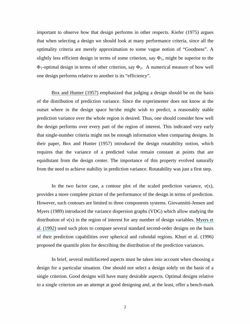
important to observe how that design performs in other respects. Kiefer (1975) argues
that when selecting a design we should look at many performance criteria, since all the
optimality criteria are merely approximation to some vague notion of “Goodness”. A
slightly less efficient design in terms of some criterion, say Φ1, might be superior to the
Φ1-optimal design in terms of other criterion, say Φ2. A numerical measure of how well
one design performs relative to another is its “efficiency”.
Box and Hunter (1957) emphasized that judging a design should be on the basis
of the distribution of prediction variance. Since the experimenter does not know at the
outset where in the design space he/she might wish to predict, a reasonably stable
prediction variance over the whole region is desired. Thus, one should consider how well
the design performs over every part of the region of interest. This indicated very early
that single-number criteria might not be enough information when comparing designs. In
their paper, Box and Hunter (1957) introduced the design rotatability notion, which
requires that the variance of a predicted value remain constant at points that are
equidistant from the design center. The importance of this property evolved naturally
from the need to achieve stability in prediction variance. Rotatability was just a first step.
In the two factor case, a contour plot of the scaled prediction variance, v(x),
provides a more complete picture of the performance of the design in terms of prediction.
However, such contours are limited to three components systems. Giovannitti-Jensen and
Myers (1989) introduced the variance dispersion graphs (VDG) which allow studying the
distribution of v(x) in the region of interest for any number of design variables. Myers et
al. (1992) used such plots to compare several standard second-order designs on the basis
of their prediction capabilities over spherical and cuboidal regions. Khuri et al. (1996)
proposed the quantile plots for describing the distribution of the prediction variances.
In brief, several multifaceted aspects must be taken into account when choosing a
design for a particular situation. One should not select a design solely on the basis of a
single criterion. Good designs will have many desirable aspects. Optimal designs relative
to a single criterion are an attempt at good designing and, at the least, offer a bench-mark
3
for efficiency studies. Properties of a good response surface design are discussed in Box
and Hunter (1957), Box and Draper (1975), Atkinson and Donev (1992) and Myers and
Montgomery (2002). Typically, one can not achieve all the ideal properties in a single
design. Therefore, there are frequently several good designs and choosing among them
involves some tradeoffs. We would like to select designs that are intuitively pleasing,
relatively easy to implement, are able to estimate all effects of interest and have good
efficiencies.
The problem of optimal experimental design for linear models (i.e. normal
responses with homogenous variances) has received much attention in the literature.
Assuming that the factor space is a p-dimensional hypercube or hypersphere with any
point inside or on the boundary of the shape being a candidate design point, standard
designs for linear models were identified. However, something other than the usual
optimal design is needed in any situation where the design space is not regular! Some
economic, practical, or physical constraints may occur on the factor settings resulting in
an irregular experimental region. One often encounters situations in which it is necessary
to eliminate some portion of the design space where it is infeasible or impractical to
collect experimental data. Hence, standard designs are not always feasible and the need
arises for best possible designs under these restrictions. Kennard and Stone (1969) were
the first to discuss in the literature the problem of irregular experimental regions and
suggested computer aided searches for selecting a design. Some case-by-case examples
of non-standard design regions are discussed in Snee (1985). Johnson and Nachtsheim
(1983) discussed how single-point augmentation procedures are helpful for finding exact
D-optimal Designs on Convex Design spaces. Recognizing the importance of computer
programs to develop designs when classical designs are not appropriate, Nachtsheim
(1987) reviewed and compared the available tools for computer-aided design of
experiments. Atkinson and Donev (1992) devoted a short chapter to restricted designs.
They used some computer algorithms to find the D-optimum design for certain irregular
regions. They emphasize that whatever the shape of the experimental region the
principles of the optimality theory remain the same. Montgomery, Loredo, Jearkpaporn,
4
and Testik (2002) give a brief tutorial on computer-aided methods for constructing
designs for irregularly shaped regions.
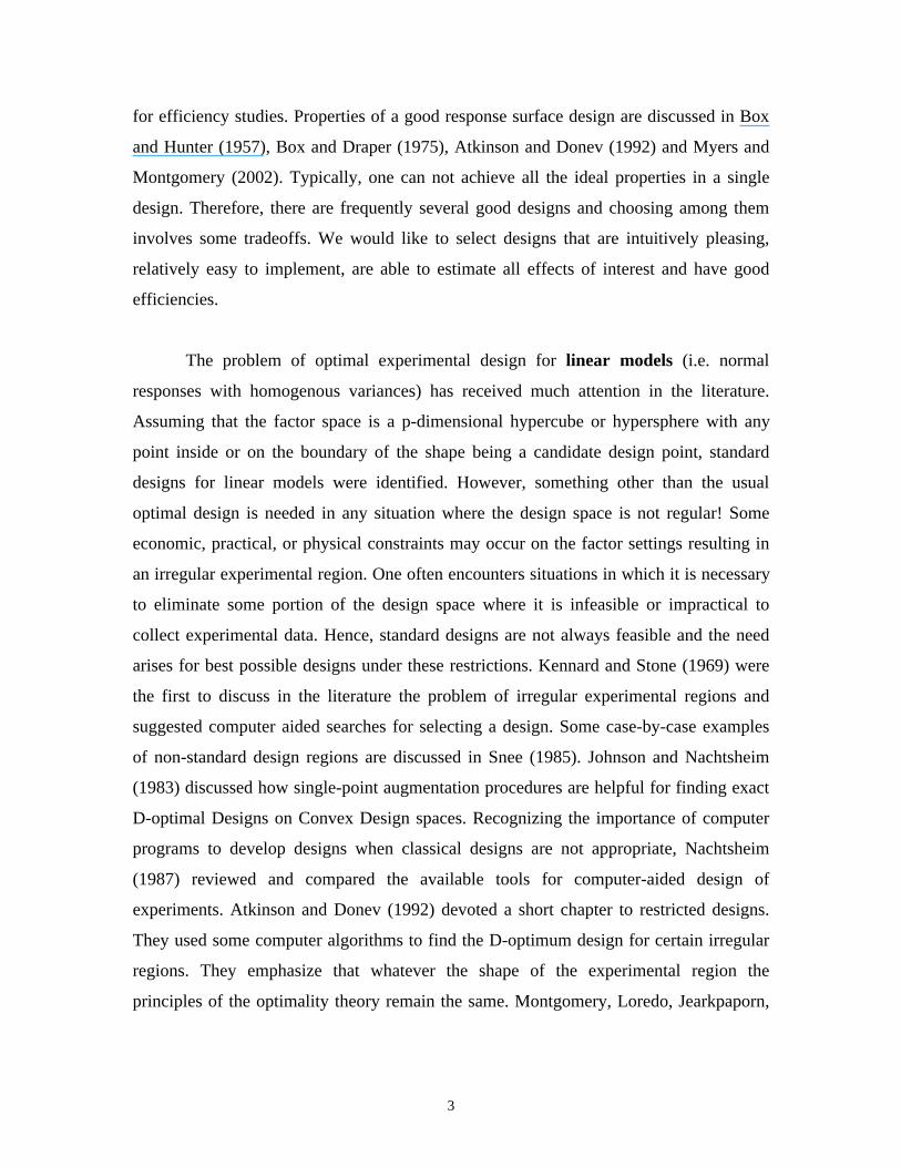
As mentioned earlier, optimal designs for linear models have been studied
extensively in the literature. The information matrix and hence the optimality function is
independent of the unknown parameters, thus optimal designs are relatively easy to find.
However, for generalized linear models (GLMs), less work has been done, because the
optimality function is a function of the unknown parameters which complicates the
process of finding an optimal design (McCullagh and Nelder, 1989).
For the one-design-variable logistic regression models, Kalish and Rosenberger
(1978) derived a D- and G-optimal design. Abdelbasit and Plackett (1983) found a D-
optimal design using the idea of two-stage model. Myers, Myers, Carter and White
(1996) introduced a two stage D-Q design. Letsinger (1995) introduced a two-stage D-D
design using a Bayesian approach in the first stage. Chaloner and Larntz (1989) took a
Bayesian approach to find robust optimal designs. A minimax procedure for finding the
optimal designs is proposed by Sitter (1992). Sitter and Wu (1993) used a different
approach to obtain characterizations of the D-, A-, and F-optimal designs for binary
response and one single variable model. F optimality deals with optimal estimation of an
ED (Effective Dose), i.e., the level of x, the drug dose, that produce a pre-specified
probability. Jia and Myers (2001) found D-optimal designs for the two-variable logistic
model in unbounded regions. Other works that considered the logistic model are Heise
and Myers (1996) and Sitter and Wu (1999).
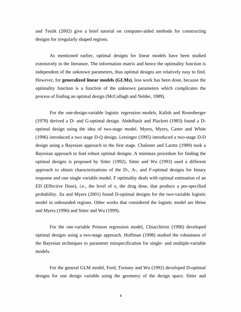
For the one-variable Poisson regression model, Chiacchirini (1996) developed
optimal designs using a two-stage approach. Huffman (1998) studied the robustness of
the Bayesian techniques to parameter misspecification for single- and multiple-variable
models.
For the general GLM model, Ford, Torsney and Wu (1992) developed D-optimal
designs for one design variable using the geometry of the design space. Sitter and

5
Torsney (1995) developed methods for deriving D-optimal design for GLM with multiple
design variables. Burridge and Sebastiani (1994) considered the multi-variable case of
GLM models for cases in which variances are proportional to the square of the mean
response. In addition, Burridge and Settimi (1998) and Dette and Wong (1999) deal with
a more general problem. Atkinson and Haines (1996) discussed locally D-optimal designs
for nonlinear models in general and GLM as well as the Bayesian approach for
optimality.
The above literature on optimality in the GLM case offers some valuable optimal
designs. However, designs that need good initial guesses, a complicated minimax
procedure, or estimation of the unknown parameters at each step to make the next move,
often seem unrealistic in practice. One wants experiments which are simple to implement
and also have ‘good’ efficiencies!
In this dissertation, we address three research projects related to optimal design:
1. We introduce a new graphical evaluation technique, which shows the stability of the
distribution of the prediction variance. The new technique focuses on how well the
design predicts for any fraction of the design space. Some second order response
surface designs are studied in terms of this new measure.
2. For the two-factor case with one corner of the square design space excluded, three
sensible alternatives designs are proposed. These designs involve reducing the factor
levels to make a smaller but standard factorial design fit or modifying the levels of
the variables at the excluded corner to locate it in the feasible design region.
Properties of these designs and relative tradeoffs are discussed. The work is also
extended to the three-factor case. Also, the alternative designs in both the two and the
three- factor cases are studied in terms of the new criteria introduced in the previous
point.
3. Study the performance of standard designs for generalized linear models. Some
results that are general to all GLMs are given. The logistic and Poisson regression
models are studied extensively.

6
I.2 Brief Review of Some Concepts in Optimality TheoryOriginally, optimality theory was introduced for linear models, where the model
of interest is1ppN1N
X)(E×××
= βy , with y a vector of N independent Normal responses
having constant variance σ2, X the design matrix, and β a vector of p unknown
parameters. Optimality theory centers around Fisher’s information matrix. One can show
that for the above model the information matrix is proportional to X’X. This matrix is
parameter free; thus, optimization in the linear models case depends only on the design
matrix.
I.2.1 Optimality Criteria and EfficiencyAs indicated earlier, many optimality criteria exist in the literature. In this
research we focus on three of them; namely, D-, G-, and Q-criterion. We begin our brief
review with the criterion used most by practitioners, namely the D-criterion.
I.2.1.1 D-Optimality The D-optimality criterion is the most often used criterion, because of its early
development and relative ease of calculation. For quantitative factors, the D-optimum
design remains unchanged with any change in the scale of the factors. The D-optimality
criterion focuses on the determinant of the information matrix. A D-optimal design
satisfies the following
)(MmaxNXX
maxDD
δδδ ∈∈
=′
where δ is a design in the design space D and N is the number of experimental runs.
)(M δ is called the moments matrix. Accordingly, the D-optimal design is that design
that maximizes the information per run. One should notice that, under independence and
normality, the determinant of the information matrix is inversely proportional to the
square of the coefficient confidence region volume. Hence, maximizing the determinant
is equivalent to minimizing the volume of the confidence region of the coefficients.
Therefore, the D-criterion addresses good parameter estimation (Myers and Montgomery,
2002).
7
To compare designs, the D-efficiency of a design, δ, is defined asp/1
*eff)(M
)(MD
=
δ
δ, where δ* is the D-optimal design.
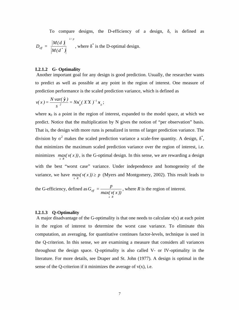
I.2.1.2 G- Optimality Another important goal for any design is good prediction. Usually, the researcher wants
to predict as well as possible at any point in the region of interest. One measure of
prediction performance is the scaled prediction variance, which is defined as
0
1
02 )XX(N)ˆvar(N
)x(v xxy −′′==
σ;
where x0 is a point in the region of interest, expanded to the model space, at which we
predict. Notice that the multiplication by N gives the notion of “per observation” basis.
That is, the design with more runs is penalized in terms of larger prediction variance. The
division by σ2 makes the scaled prediction variance a scale-free quantity. A design, δ*,
that minimizes the maximum scaled prediction variance over the region of interest, i.e.
minimizes ))x(v(max Rx∈
, is the G-optimal design. In this sense, we are rewarding a design
with the best “worst case” variance. Under independence and homogeneity of the
variance, we have p))x(v(maxRx
≥∈
(Myers and Montgomery, 2002). This result leads to
the G-efficiency, defined as
Rx
eff ))x(vmax(p
G
∈
= , where R is the region of interest.
I.2.1.3 Q-Optimality A major disadvantage of the G-optimality is that one needs to calculate v(x) at each point
in the region of interest to determine the worst case variance. To eliminate this
computation, an averaging, for quantitative continues factor-levels, technique is used in
the Q-criterion. In this sense, we are examining a measure that considers all variances
throughout the design space. Q-optimality is also called V- or IV-optimality in the
literature. For more details, see Draper and St. John (1977). A design is optimal in the
sense of the Q-criterion if it minimizes the average of v(x), i.e.

8
∫∈∈==
RDD
* dx)x(vK1
min)(Qmin)(Qδδ
δδ , where ∫=R
dxK , the volume of the design region.
The Q-efficiency is defined as )(Q
)(QminQ *
Deff δ
δδ∈= .
I.2.2 The General Equivalence Theorem for D- and G-optimum designsKiefer and Wolfowitz (1960) introduced the general equivalence theorem for
linear models. It has also been generalized for the nonlinear models (White, 1973). Many
authors discussed the theorem and its generalization. Among them are Fedorov (1972),
Silvey (1980), and Atkinson and Donev (1992).
Under very mild assumptions, the theorem states the equivalence of the following
three conditions on the optimum design, *ξ :
− *ξ is D-optimum
− *ξ is G-optimum
− the maximum prediction variance is equal to p, the number of the unknown
parameters in the model, and is achieved at the design points.
I.2.3 Orthogonality and RotatabilityOrthogonality and rotatability are two desired properties of any design.
Orthogonality is a dominant property for first-order models, while rotatability is more
important for second order models. This stems from the fact that for first order models
the primary concern is typically about what variables belong in the model. In the second
order models, more emphasis placed on the quality of the prediction rather than
estimation. In what follows we shall briefly state the definition of each property.
I.2.3.1 Orthogonality The work of Fisher (1960) emphasized that orthogonality is an important design
property. Orthogonality implies that there is no linear dependency among the design
variables as far as their levels in the experiment are concerned. For first order models, if
the design contains orthogonal variables, then the variances of the coefficients are
9
minimized when the design points are set at the extremes values of their ranges (usually,
the variables are coded to be between ±1). Hence, orthogonal designs are known as
variance optimal designs.
I.2.3.2 Rotatability Box and Hunter (1957) introduced the concept of design rotatability. A rotatable design
is one for which the scaled prediction variance remains constant at points that are
equidistant from the design center. This property does not necessarily ensure stability or
even near stability in the scaled prediction variance throughout the region. Rotatability in
the case of first order models is attainable with the standard orthogonal arrays that gave
many other important properties. Designs for second order models such as the composite
designs and other designs can be made to be rotatable. The importance of the property
has historically been tied to desire to achieve stability in prediction variance.
I.2.4 Graphical Methods for the Performance of the Prediction Capability in theRegion of InterestAs mentioned earlier, when one is interested in the stability of the scaled
prediction variance, single-value criteria may not provide a true picture of the
performance of the prediction capability of the design. In the case of two factors, a
contour plot for v(x) can be used to compare designs. However, as the number of the
factors gets larger, this plot is not easy to construct. Two graphical procedures are
introduced in the literature to study design capability of prediction for any number of
factors, k: the variance dispersion graphs (VDG) of Giovannitti-Jensen and Myers (1989)
and the quantile plots of Khuri et al. (1996). We will briefly review the VDG method.
Variance Dispersion Graph (VDG) The VDG plots the maximum, minimum, and spherical average prediction variances
versus the radius r from the center of the design throughout the region of interest. The
spherical prediction variance, Vr, is the average of the variances of the estimated
responses over the surface of a sphere, i.e. dx)x(vVr
U
r ∫=ψ , where
10
}rx:x{U 2
i
2
ir== ∑ and ∫=−
rU
1 dxψ . The stability of the prediction variance at any
given radius of spheres is illustrated by comparing the maximum prediction variance to
the minimum prediction variance. The plot also displays horizontal lines at p and 2p,
which are the 100% and 50% G-efficiencies, respectively. Thus, VDG allows the user to
see the specific locations where the prediction variance is maximized and where it is
minimized. It also gives the user the G-efficiency of the design being studied. Vining
(1993) wrote a FORTRAN program to generate the VDG for any design.
I.3 Some Response Surface DesignsIn this section a brief review of some response surface designs is given. For more
details, the reader is referred to Myers and Montgomery (2002). Response surface
methodology (RSM) frequently involves fitting a first order model εββ ++= ∑=
k
1iki0
xy
or a second order model εββββ ++++= ∑∑∑∑<== ji
jiij
k
1i
2
iii
k
1iii0
xxxxy , where y is a
measured response, xi; i=1,…,k, are the design variables, and ε is a random error with
mean 0 and variance σ2.
I.3.1 Two-Level Factorial and Fractional of Resolution III, IVFactorial designs are widely used in factor screening experiments. A special class
of factorial designs is the 2k-factorial designs, where each of the k factors has just two
levels. These designs are commonly used in the response surface methodology (RSM) to
determine which variables are important and to fit a first order model. They then become
a basic building block to create the response surface designs. However, when the number
of the variables increases, the number of runs needed to perform a complete factorial
design may exceed the experimenter’s resources. If one can assume that high-order
interaction terms are negligible, one can use a fraction of the complete factorial, which
allows estimation of the effects of interest. These designs are called fractional factorial
designs and are characterized by a resolution number, say r. A design is said to be a
fractional factorial of resolution r if no p-factor effect is aliased with another effect

11
containing less than r-p factors. One should notice that the higher the resolution the less
restrictive the assumptions are in terms of the negligible interactions. Designs of
resolution III, IV, and V are frequently considered important.
For first order models without interaction, the two-level factorials and fractional
factorials of resolution ≥ III are known to be orthogonal (Myers and Montgomery, 2002).
If some (or all) interaction terms are included in the model, the two-level factorials are
still variance optimal designs. But, one must have sufficient resolution for fractional
factorials to ensure that no model terms are aliased with each other.
For cuboidal operability regions, the two-level factorials and fractional factorials
of proper resolution are D-, G-, Q-optimal designs. However, for spherical region, they
are just D- and Q-optimal (Myers and Montgomery, 2002).
I.3.2 Second Order Model DesignsA design for a second order model must have at least 2/)1k(kk21 −++ distinct
design points and at least three levels of each design variable to estimate all the
parameters in the model. Several classes of designs were introduced to fit second order
models. We will present the four most popular classes here.
I.3.2.1 Central Composite Designs (CCD) This is the most commonly used class for second order models, developed by Box and
Wilson (1951). The CCD consists of three components: a two-level factorial or resolution
V fraction with coded factor levels at ± 1, a set of axial points at distance α from the
design center along each axis, and n0 center runs. Having two parameters, α and n0, to
select gives this class great flexibility. The region of interest influences the choice of the
axial distance, while the choice of the center runs affects the distribution of the scaled
prediction variance. A rotatable design can be achieved using 4 F=α , where F is the
number of factorial points (see Myers and Montgomery, 2002). Generally, for a spherical
region of interest, we use k=α and 3-5 center runs. For Cuboidal regions, the axial
distance is one and 1-2 center runs are used. For k=2, the design matrix is

12
−
−
−−
−−
=
00α
ααα
00
001111
1111
21 xx
DCCD
I.3.2.2 Box-Behnken Designs (BBD) Box and Behnken (1960) developed this class to be a three-level alternative to the CCD.
This class of designs is very competitive to the CCD, when spherical regions are
assumed. Actually the BBD are designed for spherical regions and should not be used if
there is interest in predicting response at the extremes. The design is near rotatable if not
rotatable. A balanced incomplete block design is used to construct the BBD when k<6;
i.e. each factor does occur in a two-level factorial structure the same number of times
with every factor. For k>5 a partially balanced incomplete block designs is implemented
using different combinations of three design factors in a factorial structure (see Myers
and Montgomery, 2002). Usually, 3-5 center runs is recommended for the BBD. The
design matrix for k=3 is as follows
′
−−−−−−−−
−−−−=
111111110000111100001111000011111111
BBDD
I.3.2.3 Small Central Composite Designs (SCD) This class was developed by Hartley (1959) as a more economical copy of the CCD. A
member of this class is always saturated or near saturated. The basic construction of the
SCD is similar to the CCD, except that the factorial component is of resolution III, rather
than resolution V. As a result, it suffers in efficiency for estimating linear effects and two
factor interactions, due to some aliasing in the factorial portion. For k=3, the design
matrix is

13
′
−−−−−−
−−−=
αααα
αα
000011110000111100001111
SCDD
I.3.2.4 Hybrid Designs Roquemore (1976) developed this class of saturated or near-saturated designs for
k=3,4,6. The Hybrid designs are very efficient and, unlike the SCD, are very competitive
to the CCD. The Hybrid designs are CCD for k-1 variables and the levels of the kth
variable are supplied in such a way as to create certain symmetries in the design. We will
consider two designs from this family: 310 and 311B, which are used when k=3. The
design matrices of these two designs are as follows:
−−−−−−
−−−−
−
=
9273.0736.109273.0736.109273.00736.19273.00736.1
6386.0116386.0116386.0116386.0111360.000
2906.100x x x
D
321
310
−−−−−−−−
−−−
−−
=
00017507.01063.211063.27507.017507.01063.211063.27507.0
17507.01063.211063.27507.017507.01063.211063.27507.0
600600
x x x
D
321
B311
I.4 Design Optimality for Generalized Linear ModelsGeneralized liner models fit regression models for a univariate response that
follows any distribution of the exponential family. The model is given by
βµiii
x)]y(E[g)(g ′== , where g(.) is the link function that connects the linear
predictor βi
x′ to the natural mean of the response variable, i
µ . See McCullagh and
Nelder (1989) and Myers et al. (2002).
14
As mentioned previously, optimality is easier to assess in the linear case than the
nonlinear case. Basically, this follows because the information matrix is just a function of
the design points in the former case, while it is a function of the unknown parameters as
well as the design points in the latter case. In generalized linear models (GLM), the
information matrix is proportional to WXX);X(I ′=β , where W is the Hessian weight
matrix, which is a function of the unknown parameters. This causes increased complexity
of design optimality in GLM. However, since the nonlinear setting is needed in many
applications, such as the chemical, biological and clinical sciences, design optimality in
GLM has been investigated, but not to a great extent.
Several solutions to the dependency of the parameters of the optimality function
were suggested in the literature. We will present these in the following subsections.
I.4.1 Locally Optimal DesignsThe simplest solution proposed in the literature to solve the parameter-
dependency problem is to assume that one can find “good” initial parameter estimates.
These estimates may come from a previous experiment or subjective guesses. Designs
found using this approach are called locally optimal designs, following the terminology
of Chernoff (1953). This approach has been considered by many authors, including
Kalish and Rosenberger (1978), Abdelbasit and Plackett (1983), Minkin (1987), and
Ford, Torsney, and Wu (1992).
This approach suffers from two main disadvantages. First, good initial estimates
are seldom available. Also, a critical point is that the criteria are generally not robust to
poor initial estimates.
I.4.2 Minimax ApproachSitter (1992) proposed the minimax approach to obtain designs that are robust to
poor initial parameter guesses. To use this approach, the experimenter determines initial
guesses for the unknown parameters as well as a specific region within which he/she
wishes the design to be robust. This approach yields designs that are more robust to poor
initial estimates of the parameters. The more uncertain the experimenter is in the initial
15
points, the more spread out is the resulting design, both in terms of coverage of the design
space and number of design points. Although, the minimax approach is difficult to
implement, it is fully automatic. A computer algorithm could be easily used.
I.4.3 Bayesian Approach Another approach to the problem is to introduce a prior distribution on the
parameters and to incorporate this prior into an appropriate design criterion. Usually, the
expectation of the design criterion is maximized over the prior distribution. A weighted
sum of the criterion values evaluated at each point could be used as an alternative to the
expectation to ease the calculations. This approach is more realistic than the local
optimality approach, since it allows several parameter values to be considered, and is less
conservative than the minimax one. A good review of the Bayesian approach is found in
Chaloner and Verdinelli (1995).
I.4.4 Sequential Designs ApproachWorking in stages could protect against poor initial parameter estimates. The idea
is to use information from earlier trials to update the parameter estimates in the next trial.
Such schemes can be useful. Usually, two-stage designs are used. Chaudhuri and
Mykland (1993) discussed the inferential problems arising from sequential procedures
and provide numerous references for this approach.
I.5 Layout of DissertationChapter II introduces a new optimality criterion that addresses good prediction. In
this chapter, some first order and second order standard designs are studied to compare
this new criterion to existing methods. Chapter III deals with non-regular operability
regions in the case of linear models for the two-factor case. The chapter ends with two
supplements. Supplement I generalizes our designs from the two-factor case to the three-
factor case. Supplement II compares the designs of the restricted design space in terms of
the new criteria introduced in Chapter II. Standard designs for generalized linear models
are discussed in Chapter IV. Some general results of the use of the standard designs in
the GLM case are presented. Examples of factorials with the Logistic and Poisson
16
regression models are investigated. Applications to real life examples are presented also.
Finally, Chapter V summarizes the results and contains topics for future research.
I.6 ReferencesAbdelbasit, K. M. and Plackett, R. L. (1983), “Experimental Design for Binary Data”,
Journal of the American Statistical Association, 78, 90-98.
Atkinson, A. C. and Donev, A. N. (1992), Optimum Experimental Designs, Oxford
University Press, Oxford.
Atkinson, A. C. and Haines, L. M. (1996), “Designs for Nonlinear and Generalized
Linear Models”, In: S. Ghosh and C.R Rao, eds., Handbook of Statistics, 13,
Elsevier Science B.V, 437-475.
Box, G.E.P. and Hunter, J.S. (1957). “Multi-factor Experimental Designs for Exploring
Response Surfaces”. Annals of Mathematical Statistics, 28, 195-241.
Box, G.E.P. and Behnken, D.W. (1960). “Some New Three-Level Designs for the Study
of Quantitative Variables”, Technometrics, 2, 455-475.
Box, G.E.P. and Draper, N.R. (1975). “Robust Designs”. Biometrika, 62, 347-352.
Burridge, J. and Sebastiani, P. (1992), “D-optimal Designs for Generalised Linear
Models”, Journal Ital. Stat. Soc., 2, 182-202.
Burridge, J. and Sebastiani, P. (1994), “D-optimal Designs for Generalised Linear
Models with Variance Proportional to the Square of the Mean”, Biometrika, 81,
295-304.
Chaloner K. and Larntz, K. (1989), “Optimal Bayesian Design Applied to Logistic
Regression Experiments”, Journal of Statistical Planning and Inference, 21, 191-
208.
Chaloner, K. and Verdinelli, I. (1995), “Bayesian Experimental Design: A Review”,
University of Minnesota Technical Report.
Chaudhuri, P. and Mykland, P. A. (1993), “Nonlinear Experiments: Optimal Design and
Inference Based on Likelihood”, Journal of the American Statistical Association,
88, 583-546.
Chernoff, H. (1953), “Locally Optimal Designs for Estimating Parameters”, Annals of
Mathematical Statistics, 24, 586-602.
17
Chernoff, H. (1979), Sequential Analysis and Optimal Designs, SIAM, Philadelphia, PA.
Chiacchirini, L.M. (1996), Experimental Design Issues in Impaired Reproduction
Studies, Ph.D. Dissertation, Virginia Tech, Blacksburg,VA.
Cornell, J. (2002) Experiments with Mixtures: Designs, Models, and the Analysis of
Mixture Data, Wiley, New York.
Dette, H. and Wong, W.K. (1999), “Optimal Designs When the Variance is a Function of
the Mean”, Biometrics, 55, 925-929
Draper, N.R. and St John, R.C. (1977), “Designs in Three and Four Components for
Mixtures Models with Inverse Terms”. Technometrics, 19, 17-130.
Dykstra, O. Jr. (1971), “The Augmentation of Experimental Data to Maximize XX ′ ”,
Technometrics, 13, 682-688.
Ehrenfeld, S. (1953), “On the Efficiency of Experimental Designs”, Annals of
Mathematical Statistics, 26, 247-255.
Fedorov, V. V. (1972), Theory of Optimal Experiments, New York: Academic Press.
Fisher, R. A. (1960), The Design of Experiments, 7th ed., Edinburgh: Oliver and Boyd.
Ford, I., Torsney, B., and Wu, C.F.J (1992), “The Use of a Canonical Form in the
Construction of Locally Optimal Designs for Nonlinear Problems”, Journal of the
Royal Statistical Society, Ser B, 54, 569-583.
Giovannitti-Jensen, A. and Myers, R.H. (1989). “Graphical Assessment of the Prediction
Capability of Response Surface Designs”. Technometrics, 31, 375-384.
Hamada, M. and Nelder, J.A. (1997), ``Generalized Linear Models for Quality-
Improvement Experiments'', Journal of Quality Technology, 29, 292-304.
Hartley, H.O. (1959). “Smallest Composite Design for Quadratic Response Surfaces”.
Biometrics, 15, 159-171.
Hebble, T.L. and Mitchell, T. J. (1972), “Repairing Response Surface Designs”,
Technometrics, 14, 767-779.
Heise, M.A. and Myers, R. H. (1996), “Optimal Designs for Bivariate Logistic
Regression”, Biometrics, 52, 613-624.
Huffman, J. W. (1998), Optimal Experimental Design for Poisson Impaired
Reproduction Studies, Ph.D. Dissertation, Virginia Tech, Blacksburg, VA.
18
Jia, Y. and Myers, R. (2001), “Design Optimality for the Two Variable Logistic
Regression Case”, submitted to Journal of Statistical Planning and Inference.
Johnson, M.E. and Nachtsheim, C. J. (1983). “Some Guidelines for Constructing Exact
D-Optimal Designs on Convex Design Spaces”. Technometrics, 25, 271-277.
Kalish, L. A. and Rosenberger, J. L. (1978), “Optimal Designs for the Estimation of the
Logistic Function”, Technical Report 33, Pennsylvania State University.
Kennard, R.W. and Stone, L. (1969). “Computer Aided Design of Experiments”.
Technometrics, 11, 298-325.
Khuri, A. Kim, H.J. and Um, Y. (1996). “Quantile Plots of the Prediction Variance for
Response Surface Designs”. Computational Statistics & Data Analysis. 22, 395-
407.
Kiefer, J. (1958), “On the Nonrandomized Optimality and Randomized Nonoptimality of
Symmetrical Designs”, Annals of Mathematical Statistics, 29, 675-699.
Kiefer, J. and Wolfowitz, J. (1959), “Optimum Designs in Regression Problems”, Annals
of Mathematical Statistics, 30, 271-294.
Kiefer, J. and Wolfowitz, J. (1960), “The Equivalence of Two Extremum Problems”,
Canadian Journal of Mathemethics,12, 363-366.
Kiefer, J. (1975), “Optimal Design: Variation in Structure and Performance Under
Change of Criterion”, Biometrika, 62, 277-288.
Lesinger, W. (1995), Optimal One and Two Stage Designs for the Logistic Regression
Model, Ph.D. Dissertation, Virginia Tech, Blacksburg, VA.
Lewis, S., Montgomery, D. and Myers R. (2001), “Examples of Designed Experiments
with Nonnormal Responses”, Journal of Quality Technology, 33, 265-278.
Martin, B., Parker, D. and Zenick, L. (1987), “Minimize Slugging by Optimizing
Controllable Factors on Topaz Windshield Modeling”, Fifth Symposium on
Taguchi Methods. American Supplier Institute, Inc., Dearborn, MI, 519-526.
McCullagh, P. and Nelder, J.A. (1989), Generalized Linear Models, 2nd edition, New
York, Chapman and Hall.
Minkin, S. (1987), “Optimal Designs for Binary Data”, Journal of the American
Statistical Association, 82,1098-1103.
19
Montgomery, D. C. , Loredo, E. N., Jearkpaporn, D., Testik, M.C. (2002). “Experimental
Designs for Constrained Regions”. To appear in Quality Engineering.
Myers, R. H., Vining, G.G., Giovannitti-Jensen, A. and Myers, S.L. (1992). “Variance
Dispersion Properties of Second-Order Response Surface Designs”. Journal of
Quality Technology, 24, 1-11.
Myers, R.H. and Montgomery, D. C. (1997), “A Tutorial on Generalized Linear Models”,
Journal of Quality Technology, 29, 274-291.
Myers, R.H. and Montgomery, D. C. (2002), Response Surface Methodology: Process
and Product Optimization Using Designed Experiments, 2nd edition, Wiley.
Myers, R.H., Montgomery, D. C., and Vining, G.G. (2002), Generalized Linear Models
with Applications in Engineering and the Sciences, Wiley Series in Probability and
Statistics.
Myers, W. R., Myers, R.H., and Carter, W.H. Jr. (1994), “Some Alphabetic Optimal
Designs for the Logistic Regression Model”, Journal of Statistical Planning and
Inference, 42, 57-77.
Myers, W. R., Myers, R.H., Carter, W.H. Jr., and White, K. L. (1996), “Two Stage
Designs for the Logistic Regression Model in a Single Agent Bioassay”, Journal of
Biopharmaceutical Statistics, 6(4).
Nachtsheim, C. J. (1987). “Tools for Computer-Aided Design of Experiments”. Journal
of Quality Technology, 19, 132-160.
Pazman, A.(1986), Foundation of Optimum Experimental Design, Reidel, Dordrecht.
Pukelsheim, F. (1993), Optimal Design of Experiments, Wiley, New York.
Roquemore, K.G. (1976). “Hybrid Designs for Quadratic Response Surfaces”.
Technometrics, 18, 419-423.
Sebastiani, P. and Settimi, R. (1998), “First-order Optimal Designs for Non-linear
Models”, Journal of Statistical Planning and Inference, 74, 177-192.
Shah, K. R. and Sinha, B. K (1989), Theory of Optimum Design. Lecture Notes in
Statistics 54, Springer, Berlin.
Silvey, D. (1980), Optimal Design, Chapman and Hall, London.
Sitter R. R. (1992), “Robust Designs for Binary Data”, Biometrics, 48, 1145-1155.
20
Sitter R. R. and Torsney, B. (1995), “D-Optimal Designs for Generalized Linear
Models”, In: C.P. Kitsos and W.G. Müller, eds., MODA 4 - Advances in Modern
Data Analysis: Proceedings (the 4th international wokshop in Spetses, Greece, June
5-9, 1995). Heidelberg, Germany: Physica-Verlag, 87-102.
Sitter, R. R. and Wu, C. F. J. (1993), “On the Accuracy of Fieller Intervals for Binary
Response Data”, Journal of the American Statistical Association, 88, 1021-1025.
Sitter, R. R. and Wu, C. F. J. (1999), “Two-Stage Design of Quantal Response Studies”,
Biometrics, 55,396-402
Smith, K. (1918), “On the Standard Deviations of Adjusted and Interpolated Values of an
Observed Polynomial Function and its Constants and the Guidance they Give
Towards a Proper Choice of the Distribution of Observations”, Biometrika, 12, 1-
85.
Snee, R.D.(1985), “Computer-Aided Design of Experiments – Some Practical
Experiences”. Journal of Quality Technology, 17, 222-236.
Wald, A. (1943), “On the Efficient Design of Statistical Investigation”, Annals of
Mathematical Statistics, 14,134-140.
White, L. (1973), “An Extension of the General Equivalence Theorem to Nonlinear
Models”, Biometrika, 60, 345-348.
Zacks, S. (1971), The Theory of Statistical Inference, Wiley, NY.
21
Chapter II Fraction of Design Space to Assess the Prediction
Capability of Response Surface Designs
II.1 AbstractVariance Dispersion Graphs (VDGs) are useful summaries for comparing
competing designs on a fixed design space. However, they might not give all the
information about the prediction capability of the design. The Fraction of Design Space
(FDS) technique is proposed, which addresses some of the shortcomings of VDGs. The
new technique is comprised of two tools that give the researcher more detailed
information by quantifying the fraction of design space where the scaled predicted
variance (SPV) is less than or equal to any pre-specified value. The Fraction of Design
Space Graph (FDSG) gives the researcher information about the distribution of the SPV
in the region based on the ranges and proportions of possible SPV values. The second
tool, the Scaled FDS graph (SFDSG), is used for comparing the overall stability of the
prediction performance. The FDS technique complements the VDGs to give the
researcher more insight about the prediction capability of the design. Several standard
designs with different numbers of factors are studied with both methods: VDG and FDS.
Keywords: Alphabetical criteria, stability of scaled prediction variance, VDG, FDS
technique, FDSG, SFDSG
II.2 Introduction
One measure of prediction performance is the scaled prediction variance (SPV) or
v(x), which is defined for a particular location in the design space by
01
020 )XX(N)ˆvar(N
)x(v xxy −′′==
σ; where x0 is a point in the region of interest,
expanded to the model space, at which we predict. For example, for a design involving
two factors and a second order model the point (x10, x20) would expanded to
22
)xx,x,x,x,x,1( 2010220
21020100 =x . The use of N, the total sample size, adjusts the SPV to
be measured on a per observation basis, and allows for fair comparisons between designs
of different sizes. Two existing optimality criteria address prediction performance: G-
and Q-optimality criteria. Q-optimality is also called V- or IV-optimality in the literature
(Draper & St. John, 1977). However, these single-valued criteria do not reveal the true
complexities of design prediction capability. The approach of looking only at design
moments can be sometimes misleading, since how the moments are achieved is more
important. Box and Hunter (1957) emphasized that judging a design should be on the
basis of the distribution of SPV. Since the experimenter does not know at the outset
where in the design space he/she might wish to predict, a reasonably stable SPV over the
whole region is desired. Thus, one should consider how well the design performs over
every part of the region of interest. This highlighted very early that single-number criteria
might not be enough information when comparing designs. In their paper, Box and
Hunter (1957) introduced the notion of design rotatability, which requires that the
variance of a predicted value remain constant at points that are equidistant from the
design center. Rotatability was just a first step, as the importance of this property evolved
naturally from the need to achieve stability in SPV.
In the two factor case, a contour plot of the SPV, v(x), provides a complete picture
of the performance of the design in terms of prediction. However, the practicality of such
contours is limited to three components systems. Giovannitti-Jensen and Myers (1989)
introduced variance dispersion graphs to assess the overall prediction capability of a
response surface design inside a region of interest. These graphs consist of the maximum
and minimum SPV values and the spherical average of the SPV on spheres inside the
design region, R, against their radii. Myers, Vining, Giovannitti-Jensen and Myers (1992)
used such plots to compare several standard second–order designs on the basis of their
prediction capabilities over spherical and cuboidal regions. As with any plot that reduces
the dimensionality of the information, the VDGs can not provide complete information
concerning the distribution of the SPV on a given sphere. Thus, they may not enable the
user to discriminate between two designs that have similar VDG patterns but different
SPV distributions on the sphere.
23
Khuri et al. (1996) proposed the quantile plots for describing the distribution of
the SPV. A curve of the cumulative distribution of the SPV at each radius is created to
compare designs at each radius or to study the properties of a specific design. Although,
the quantile plots do supply more information on the distribution of the SPV at a given
radius, they do not alleviate the problems that exist with the VDGs. Also, quickly the
number of graphs becomes impractically large.
Both the VDG and the Quantile plots do not take into account the volume of the
sphere and the proportion of the design space at various distances from the center of the
design space. They deal with the SPV on a sphere of radius r but ignore the volume
associated with this information. The VDG transforms the information of the sphere to a
point at its three curves (minimum and maximum of v(x) and the spherical variance
curves), while the Quantile plot transfers this information to a single curve representing
the cumulative distribution of v(x) at each sphere. Thus, the information of each sphere is
given the same “weight” in these graphs. But the weight of each piece of information is
not equal in general, and one should weigh this information by the volume of the
corresponding sphere. Figure II.1 depicts the relative change in volume corresponding to
sphere of radius r for two-, four- and six-factor designs. The relative contribution to the
overall volume of the region is an increasing function in r. When the dimension, k, of the
design increases, the size of the relative contribution diminishes for small r and enlarges
for large r. Figure II.1 considers a spherical region and displays how a quickly increasing
fraction of the design space is associated with the outer edges of the space as k increases.
This means that fewer points at large values of radii on the VDG curves and fewer curves
corresponding to large r in the Quantile plots dominate the prediction capability; and
should be given more weight in our interpretation of these graphs.
24
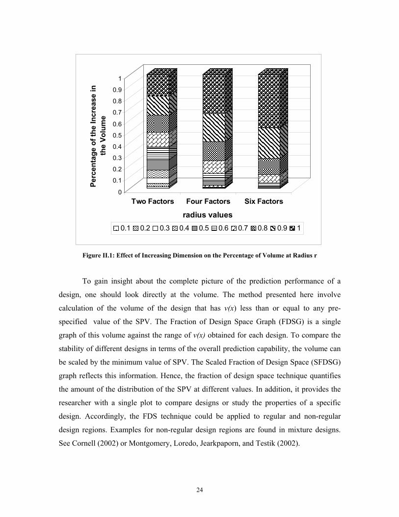
Figure II.1: Effect of Increasing Dimension on the Percentage of Volume at Radius r
To gain insight about the complete picture of the prediction performance of a
design, one should look directly at the volume. The method presented here involve
calculation of the volume of the design that has v(x) less than or equal to any pre-
specified value of the SPV. The Fraction of Design Space Graph (FDSG) is a single
graph of this volume against the range of v(x) obtained for each design. To compare the
stability of different designs in terms of the overall prediction capability, the volume can
be scaled by the minimum value of SPV. The Scaled Fraction of Design Space (SFDSG)
graph reflects this information. Hence, the fraction of design space technique quantifies
the amount of the distribution of the SPV at different values. In addition, it provides the
researcher with a single plot to compare designs or study the properties of a specific
design. Accordingly, the FDS technique could be applied to regular and non-regular
design regions. Examples for non-regular design regions are found in mixture designs.
See Cornell (2002) or Montgomery, Loredo, Jearkpaporn, and Testik (2002).
0
0.1
0.2
0.3
0.4
0.5
0.6
0.7
0.8
0.9
1
Perc
enta
ge o
f the
Incr
ease
in
the
Volu
me
Two Factors Four Factors Six Factors
radius values0.1 0.2 0.3 0.4 0.5 0.6 0.7 0.8 0.9 1
25
The outline of the paper is as follows. Section II.3 includes a brief review of the
VDG technique. In Section II.4, the Fraction of Design Space technique with the FDSG
and SFDSG plots is described. Section II.5 evaluates some second-order designs and
compares them using FDS and VDG over spherical regions. For cuboidal regions, two
second-order designs are discussed in Section II.6.
II.3 Review of Variance Dispersion Graphs (VDG)
Giovannitti-Jensen and Myers (1989) introduced a variance-based graphical
approach to study the prediction capability of a design. The VDG plots the maximum,
and minimum over spheres of radius r from the center, as well as the spherical average of
the SPV against the radius r from the center of the design throughout the region of
interest. The spherical average variance is defined by dx)x(vVr
U
r ∫=ψ , where
}rx:x{U 2
i
2
ir== ∑ and ∫=−
rU
1 dxψ . For cuboidal regions, the above three statistics are
calculated over spheres or portions of spheres that are on or within the cube. The
rotatability of the SPV at any given radius of spheres is illustrated by comparing the
maximum to the minimum of SPV across the range of radii. The plot also displays
horizontal lines at p and 2p, which are the 100% and 50% G-efficiencies, respectively.
Vining (1993) wrote a FORTRAN program to generate the VDG for any design.
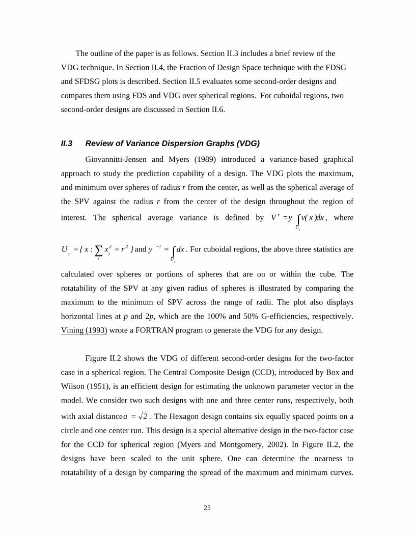
Figure II.2 shows the VDG of different second-order designs for the two-factor
case in a spherical region. The Central Composite Design (CCD), introduced by Box and
Wilson (1951), is an efficient design for estimating the unknown parameter vector in the
model. We consider two such designs with one and three center runs, respectively, both
with axial distance 2=α . The Hexagon design contains six equally spaced points on a
circle and one center run. This design is a special alternative design in the two-factor case
for the CCD for spherical region (Myers and Montgomery, 2002). In Figure II.2, the
designs have been scaled to the unit sphere. One can determine the nearness to
rotatability of a design by comparing the spread of the maximum and minimum curves.
26
As in Figure II.2, if the maximum, minimum and average curves are all identical, the
designs are rotatable. By comparing the maximum SPV value for the design to the 100%
G-efficiency line in Figure II.2, it appears that the Hexagon and the CCD with three
center runs are about 86% G-efficient, whereas the CCD with one center run is just 67%
G-efficient. The VDG also allows the user to see the specific locations where the SPV is
maximized and where it is minimized. The Hexagon performs better than the CCD with
one center run almost over the whole region. But, the CCD with three center runs
performs best when 8.0r < . If the relative change in the design volume was constant
with the change in r, one could conclude that the CCD with three center runs performs
better throughout a large portion of the design region. However, since the fraction of the
design space is changing as we change the associated radius, a precise comparison is not
easily possible.
0 0.2 0.4 0.6 0.8 1radius
5
10
15
20
CCD-1CR
HexagonCCD-3CR
50% G-eff
100% G-eff
Figure II.2: VDG of some Two-Factor Designs
II.4 The Fraction of Design Space Criterion (FDS)It is proposed that one can assess the prediction performance of a design or
compare different designs based on the fraction of the design space contained within a
27
variety of cut-off points for SPV. The larger the fraction of design space at or below a
given value, the better the design. For purposes of comparisons among the different
designs, we considered the cut-off point contour volume relative to the design region
volume. For a practitioner who does not know a priori where in the design space he/she
may wish to predict, having a large area relatively close to the minimum of the SPV is
highly desirable. Two graphs can be created to assess the prediction capability. The first
one, the Fraction of Design Space Graph (FDSG), plots the fraction of design space
values against the entire range of cut-off points ranging from the minimum to the
maximum of SPV. This allows the researcher to evaluate the performance of designs in
terms of prediction. When several designs are plotted on the same graphs, it allows the
researcher to see the global minimum and global maximum of SPV of each design. The
slope of the curve shows how quickly the design reaches the maximum value of the SPV,
with closer to vertical being preferred. The 50% and 100% G-efficiency lines are also
shown vertically on this graph, which allows the researcher to determine the approximate
G-efficiency of each design. The second graph, the Scaled Fraction of Design Space
Graph (SFDSG), compares the overall stability of different designs by first plotting the
fraction of design space against the standardized or scaled cut-off points. The scaled cut-
off point is defined as ))x(v(min
vv
0R
s = , where the minimum SPV for each individual
design is used. The steeper the slope of the curve is the more stable the SPV of the
design. This graph also allows direct access to the ratio of maximum to minimum SPV.
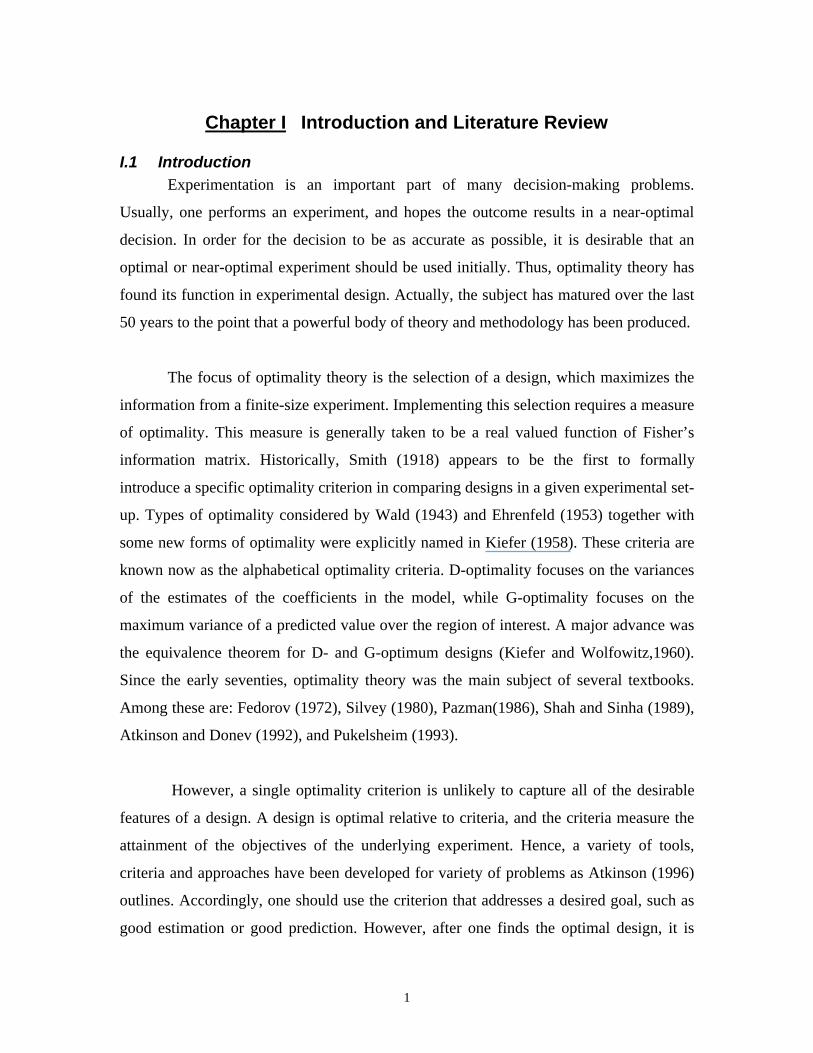
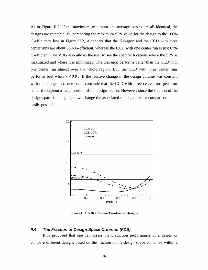
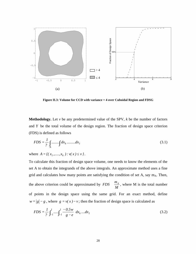
Consider the CCD in two variables over a cuboidal region with one center run.
We are interested in the fraction of design that has SPV no more than 4. Note that for this
design 25.7)x(v2.3 0 ≤≤ . The volume of the cut-off point (4) contour is shown in
Figure II.3a and represents 56% of the total design space. In Figure II.3b, this becomes
the point (4, 56%) on the FDSG. Similarly, for any chosen cutoff for the SPV, we can
obtain the fraction of design space at or below this value.
28
Figure II.3: Volume for CCD with variance = 4 over Cuboidal Region and FDSG
Methodology. Let v be any predetermined value of the SPV, k be the number of factors
and Ψ be the total volume of the design region. The fraction of design space criterion
(FDS) is defined as follows
∫ ∫=A
1k dx.........dx........?1
FDS (3.1)
where }v)x(v:)x,.....,x{(A k1 ≤= .
To calculate this fraction of design space volume, one needs to know the elements of the
set A to obtain the integrands of the above integrals. An approximate method uses a fine
grid and calculates how many points are satisfying the condition of set A, say mA. Then,
the above criterion could be approximated by Mm
FDS A≅ , where M is the total number
of points in the design space using the same grid. For an exact method, define
ggw −= , where v)x(vg −= ; then the fraction of design space is calculated as
1k1
1
1
1dx....dx
g w5.0
.....?1
FDS ∫ ∫− − −−
=ε
(3.2)
-1 -0.5 0 0.5 1-1
-0.5
0
0.5
1
> 4
≤ 4
(a) (b)
2 4 6 8Variance
56%
Fra
ctio
nof
Des
ign
Spa
ce
29
where ε is a small number used to ensure that the denominator is greater than zero.
Notice that the set A could be defined in terms of g as follows }0g:)x,....,x{(A k1 <= .
Hence, we are interested in negative values of g. Actually w is merely an indicator
function with two values, either -2g or 0. It filters out all the variances greater than the
cut-off points and allows integration over the entire range of the variables.
For rotatable designs in a spherical region the above criterion is simplified to
∫ −
−−
=1
0
1k drrg
w5.0kFDS
ε; where r is the radius of the region scaled to the unit sphere.
The following two sections contain some second order designs evaluated by both
the VDG and the FDS techniques over spherical and cuboidal regions. The ability of the
FDS to highlight different information of the prediction performance of the design than
the VDGs is discussed. A FORTRAN code available from the authors has been
developed for calculating the FDSG and SFDSG. It uses an IMSL multivariate numerical
integration subroutine.
II.5 Comparisons of the Standard Second-Order Designs over SphericalRegion
The CCD design, mentioned in Section II, contains three main components: a
two-level factorial, or a resolution V fraction, a set of axial points at distance α from the
center of the design along each axis and n0 center runs. Unless otherwise specified, we
will use the most commonly selected value k=α . Three other popular classes of
second-order designs are considered in this paper: the Box-Behnken (BBD), the Small
Composite (SCD) and the Hybrid designs. Box and Behnken (1960) developed the BBD
to be a three-level alternative to the CCD. These designs are competitive with the CCD
when the region of interest is spherical. Hartley (1959) introduced the Small Composite
Designs (SCD). These designs have the same construction as the CCD except they
employ a resolution III factorial design in the factorial portion. These designs are often
near-saturated and are more economical than the CCD. Another near-saturated class of
30
designs is the Hybrid class (Roquemore, 1976). These designs are available for k=3,4,
and 6. This class contains some designs that are highly efficient and near-rotatable.
II.5.1 Example: Two Factors on Spherical RegionThe FDSG for the three designs with two Factors on a spherical region discussed in
Section II and Figure II.2 is shown in Figure II.4a. Now the superiority of the CCD with
three center runs is demonstrated over the whole region since for any value of SPV, it has
the largest fraction of the design space at or below this level. Also, the fact that the
Hexagon and CCD with one center run differ consistently in overall performance is
highlighted in the FDSG. The new plot allows global comparisons more easily than the
VDGs, which encourage comparisons at fixed radii. Notice how the maximum and
minimum values of the designs occur at different radii of the VDGs and with different
associated volumes. Figure II.4b shows that the Hexagon is more stable than the CCD
with either of center runs combinations, since it has the steepest slope.
II.5.2 Example: Three Factors on Spherical RegionFigure II.5 shows the VDG for some second-order designs in three factors. The CCD
with three center runs (N=17) is near rotatable and performs consistently on a sphere for
large radii. The BBD with three center runs (N=15) is a competitor to the CCD near the
perimeter and is better at lower values of r. The SCD (N=13) is best near the center, but it
suffers badly when the radius gets bigger. For the Hybrid designs, the H311B is near
rotatable and performs better than H310 for large radii. The FDSG and SFDSG in Figure
II.6 show that the rapidly increasing maximum SPV at the edges of the design for the
SCD and H310 make the designs much less desirable. The CCD is better at the edges
relative to the BBD, which is better near the center of the design. However, there is
relatively little fraction of the design near the center. The FDSG shows that for the
majority of the SPV values the CCD design is best but the BBD, CCD, and H311B are
very close in their prediction performance. The CCD is more stable than the other designs
as shown by the SFDSG.
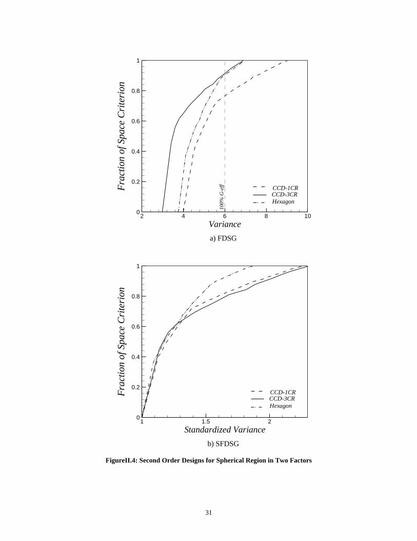
31
FigureII.4: Second Order Designs for Spherical Region in Two Factors
2 4 6 8 10Variance
0
0.2
0.4
0.6
0.8
1
Frac
tion
ofSp
ace
Cri
teri
on
CCD-1CR
HexagonCCD-3CR
100%
G-e
ff
a) FDSG
1 1.5 2Standardized Variance
0
0.2
0.4
0.6
0.8
1
Frac
tion
ofSp
ace
Cri
teri
on
CCD-1CR
HexagonCCD-3CR
b) SFDSG
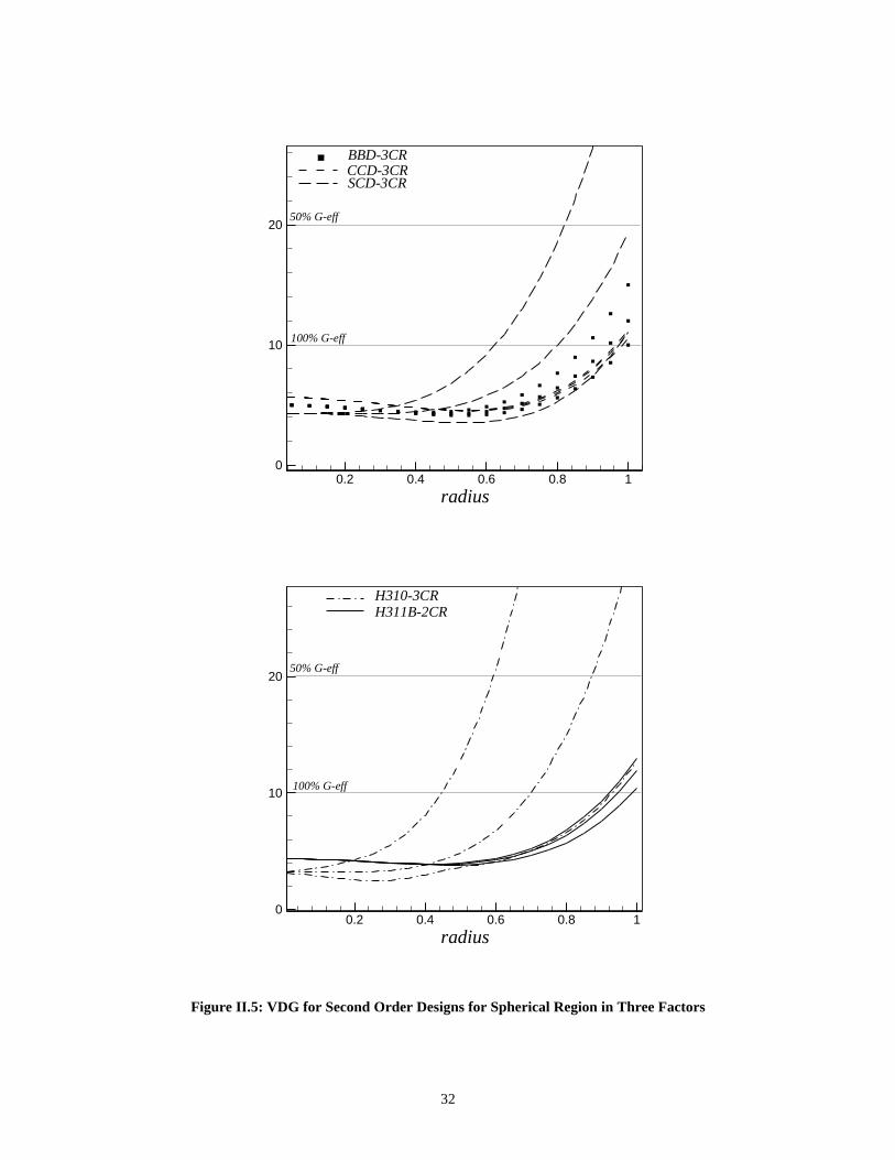
32
Figure II.5: VDG for Second Order Designs for Spherical Region in Three Factors
0.2 0.4 0.6 0.8 1radius
0
10
20
BBD-3CR
SCD-3CRCCD-3CR
100% G-eff
50% G-eff
0.2 0.4 0.6 0.8 1radius
0
10
20
H311B-2CRH310-3CR
100% G-eff
50% G-eff
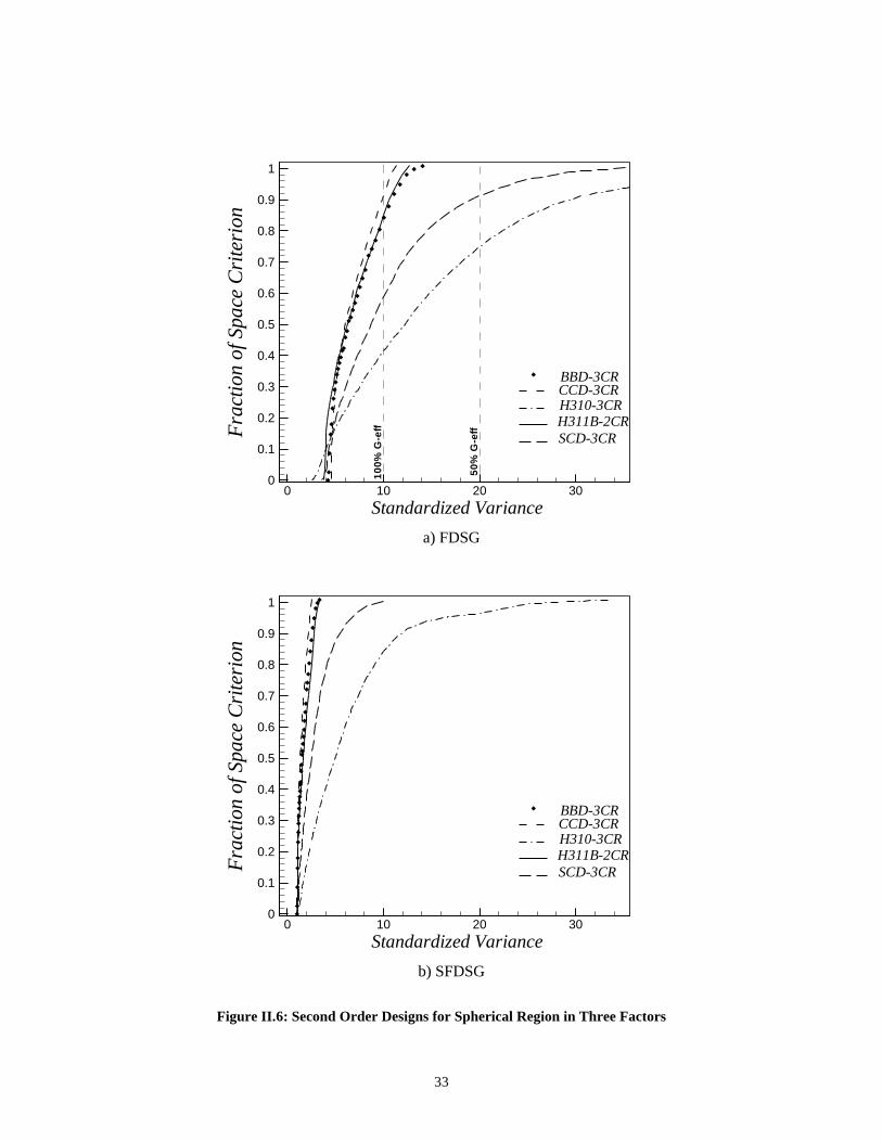
33
Figure II.6: Second Order Designs for Spherical Region in Three Factors
0 10 20 30Standardized Variance
0
0.1
0.2
0.3
0.4
0.5
0.6
0.7
0.8
0.9
1
Frac
tion
ofSp
ace
Cri
teri
on
BBD-3CR
H311B-2CRH310-3CR
SCD-3CR
CCD-3CR
50%
G-e
ff
100%
G-e
ff
a) FDSG
0 10 20 30Standardized Variance
0
0.1
0.2
0.3
0.4
0.5
0.6
0.7
0.8
0.9
1
Frac
tion
ofSp
ace
Cri
teri
on
BBD-3CR
H311B-2CRH310-3CR
SCD-3CR
CCD-3CR
b) SFDSG

34
II.5.3 Example: Four Factors on Spherical RegionFor the four factor case, the BBD is a rotation of the CCD (N=27). Therefore, their VDG
in Figure II.7 are identical, and both designs are rotatable. The designs perform
considerably better than the SCD (N=19) for large values of r. For all the above four
factor designs three center runs are used. The BBD and the CCD are highly efficient in
the G-sense (95%), while the SCD is just 25% G-efficient. The SCD suffers because it
uses a resolution III in its factor portion, which results in correlation between the linear
and the two factor interaction terms. For the Hybrids, the performance of H416A and
H416C is close to each other, with the first design nearer to rotatability. On the average
H416B performs best with lower SPV for 5.0r ≤ . In all of these Hybrids a total number
of three center runs is used (N=19). Note that in the original design matrix (N=16) of
H416C contains one center run and we added two other center runs to get a total of three.
Figure II.8 shows that the three Hybrids have smaller minimum SPV than the BBD, CCD
and SCD, but higher maximum than the BBD and the CCD. The H416C is almost
uniformly better than the other two hybrids. This information is more easily extracted
from the FDSG than from the VDGs, which are cluttered with multiple lines for each
design. From the SFDSG, one realizes that the BBD and CCD are more stable than all the
other designs. The SCD is the worst design in terms of the G-efficiency and is non-stable.
The H416C is the most stable design among the hybrid designs.
II.5.4 Example: Five Factors on Spherical RegionFigure II.9 displays the VDG of three designs for the five-variable case: BBD (N=45) and
two CCD (N=31) designs with a half fraction resolution V factorial. Different α values
are considered for the two CCD designs with 5=α and 2=α , which results in a
rotatable design. All three designs are augmented with five center runs. Both CCDs
perform better than the BBD near the center of the region, with the rotatable CCD (CCD-
R) being slightly better than the nonrotatable one (CCD-NR). The best design near the
perimeter of the region is CCD-NR. The BBD is 55% G-efficient, while CCD-R and
CCD-NR are 77% and 79% efficient, respectively.
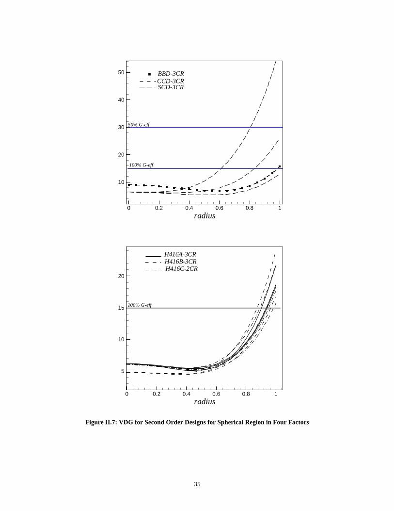
35
Figure II.7: VDG for Second Order Designs for Spherical Region in Four Factors
0 0.2 0.4 0.6 0.8 1radius
10
20
30
40
50 BBD-3CR
SCD-3CRCCD-3CR
100% G-eff
50% G-eff
0 0.2 0.4 0.6 0.8 1radius
5
10
15
20
H416A-3CR
H416C-2CRH416B-3CR
100% G-eff
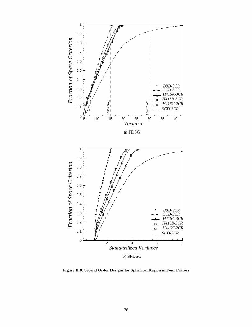
36
Figure II.8: Second Order Designs for Spherical Region in Four Factors
5 10 15 20 25 30 35 40Variance
0
0.1
0.2
0.3
0.4
0.5
0.6
0.7
0.8
0.9
1
Frac
tion
ofSp
ace
Cri
teri
on
A
A
A
A
A
A
A
B
B
B
B
B
B
B
B
C
C
C
C
C
C
C
ABC
BBD-3CR
H416B-3CRH416A-3CR
H416C-2CR
CCD-3CR
SCD-3CR10
0%G
-eff
50%
G-e
ff
a) FDSG
2 4 6 8Standardized Variance
0
0.1
0.2
0.3
0.4
0.5
0.6
0.7
0.8
0.9
1
Frac
tion
ofSp
ace
Cri
teri
on
A
A
A
A
A
A
A
B
B
B
B
B
B
B
B
C
C
C
C
C
C
C
ABC
BBD-3CR
H416B-3CRH416A-3CR
H416C-2CR
CCD-3CR
SCD-3CR
b) SFDSG
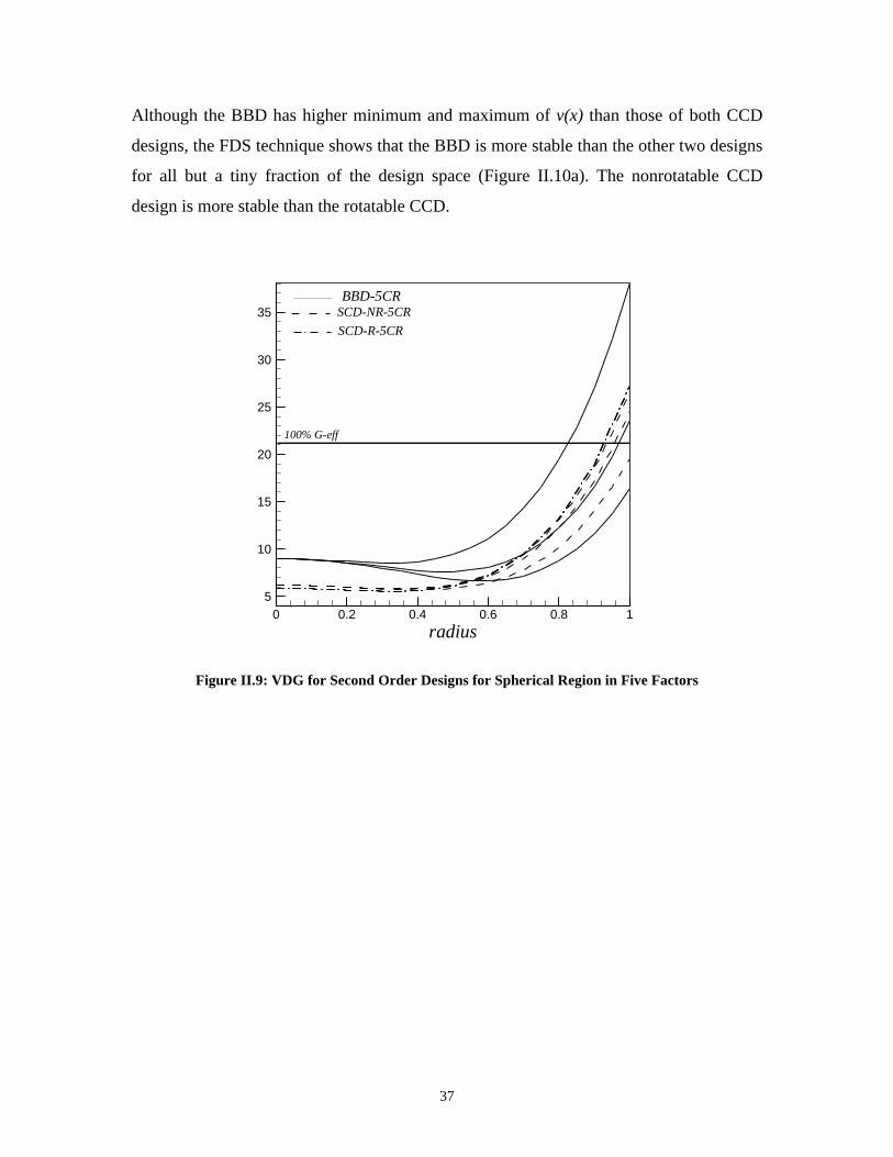
37
Although the BBD has higher minimum and maximum of v(x) than those of both CCD
designs, the FDS technique shows that the BBD is more stable than the other two designs
for all but a tiny fraction of the design space (Figure II.10a). The nonrotatable CCD
design is more stable than the rotatable CCD.
0 0.2 0.4 0.6 0.8 1radius
5
10
15
20
25
30
35BBD-5CR
SCD-R-5CRSCD-NR-5CR
100% G-eff
Figure II.9: VDG for Second Order Designs for Spherical Region in Five Factors
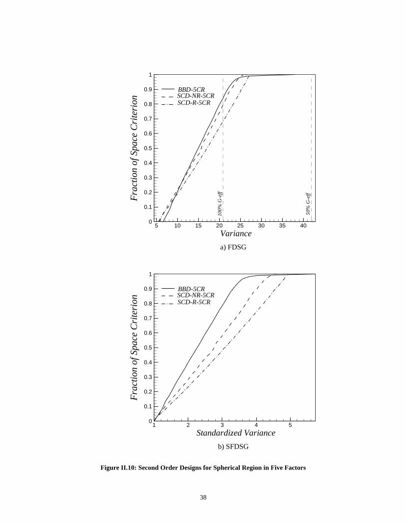
38
Figure II.10: Second Order Designs for Spherical Region in Five Factors
5 10 15 20 25 30 35 40Variance
0
0.1
0.2
0.3
0.4
0.5
0.6
0.7
0.8
0.9
1
Frac
tion
ofSp
ace
Cri
teri
on
BBD-5CR
SCD-R-5CRSCD-NR-5CR
100%
G-e
ff
50%
G-e
ff
a) FDSG
1 2 3 4 5Standardized Variance
0
0.1
0.2
0.3
0.4
0.5
0.6
0.7
0.8
0.9
1
Frac
tion
ofSp
ace
Cri
teri
on
BBD-5CR
SCD-R-5CRSCD-NR-5CR
b) SFDSG

39
II.5.5 Example: Six Factors on Spherical RegionTwo rotatable designs in the six-factor case are considered here: CCD with four center
runs (N=48) and the hybrid H628A with additional two center runs (N=30). Figure II.11,
shows that the hybrid is better than CCD over a considerable portion of the region
( 8.0r ≤ ), while both designs have the same prediction capability near the perimeter of
the region. This difference looks quite dramatic on the VDG but Figure II.12a, indicates
that both designs have almost the same performance over the whole region reflecting the
very small fraction of the design space right near the center of the design. Actually, the
portion of design region where the hybrid performs better contains less than 15% fraction
of design space as can be seen from Figure II.1. Figure II.12b shows that the CCD is
superior to the hybrid design in terms of the stability of the SPV distribution. This
difference is primarily attributable to the smaller minimum SPV for the Hybrid design.
0 0.2 0.4 0.6 0.8 1radius
5
10
15
20
25
30
35CCD-4CR
H628A-2CR
100% G-eff
FigureII.11: VDG for Second Order Designs for Spherical Region in Six Factors
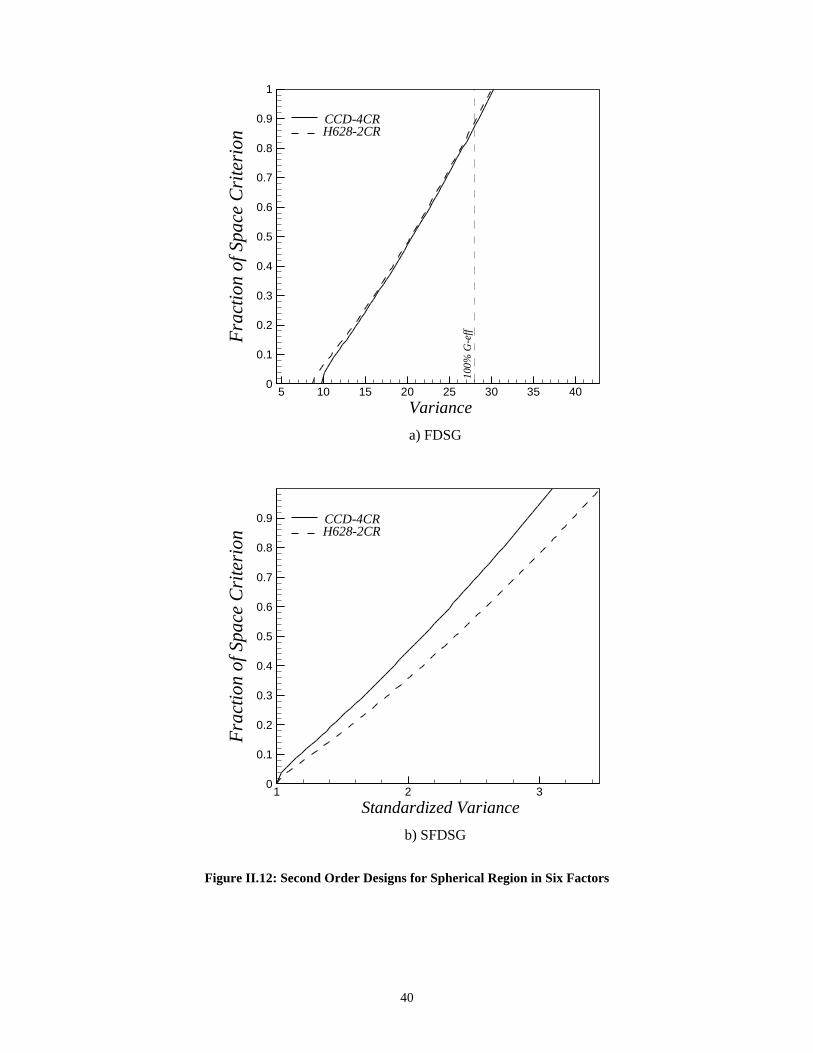
40
Figure II.12: Second Order Designs for Spherical Region in Six Factors
5 10 15 20 25 30 35 40Variance
0
0.1
0.2
0.3
0.4
0.5
0.6
0.7
0.8
0.9
1
Frac
tion
ofSp
ace
Cri
teri
on
CCD-4CRH628-2CR
100%
G-e
ff
a) FDSG
1 2 3Standardized Variance
0
0.1
0.2
0.3
0.4
0.5
0.6
0.7
0.8
0.9
Frac
tion
ofSp
ace
Cri
teri
on
CCD-4CRH628-2CR
b) SFDSG

41
II.6 Comparisons of the Standard Second-Order Models over CuboidalRegion with Three FactorsAn important second-order design for cuboidal regions is the CCD with α=1 which is
known as “face center cube“. Many other highly D-efficient designs are available for
cuboidal regions but are not commonly used in practical applications. In this section we
compare two designs of equal size: the CCD with one center run and the BBD with three
center runs in three factors. Note that the BBD has no points on the corners of the cube.
All the points are on a sphere of radius 2 except the center runs, while the vertices of
the region reside on a radius of 3 . This results in large SPV at the perimeter of the
region for this design. However, the BBD is competitive with the CCD for radius values
less than 2 as the VDG indicates (see Myers et al, 1992). Figure II.13a indicates that
the CCD is better than the BBD for almost the whole cube. However, there are some SPV
values between 6 and 7 where more of the design space curve is predicted well by the
BBD. In terms of the overall stability of the prediction performance, Figure II.13b shows
that there is no clear winner.
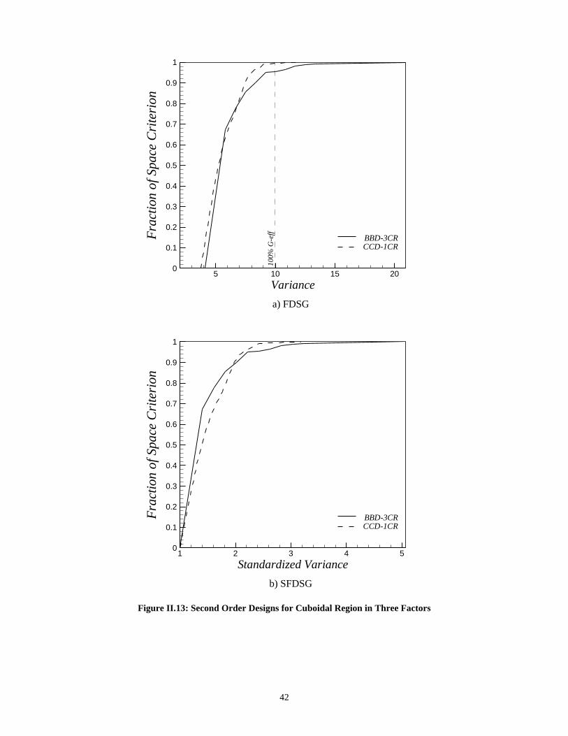
42
Figure II.13: Second Order Designs for Cuboidal Region in Three Factors
5 10 15 20Variance
0
0.1
0.2
0.3
0.4
0.5
0.6
0.7
0.8
0.9
1
Frac
tion
ofSp
ace
Cri
teri
on
BBD-3CRCCD-1CR
100%
G-e
ff
a) FDSG
1 2 3 4 5Standardized Variance
0
0.1
0.2
0.3
0.4
0.5
0.6
0.7
0.8
0.9
1
Frac
tion
ofSp
ace
Cri
teri
on
BBD-3CRCCD-1CR
b) SFDSG
43
II.7 ConclusionsAlphabetic optimality criteria, such as G- and Q-Optimality, as well as variance
dispersion graphs are all useful measures for comparing competing designs. The Fraction
of Design Space (FDS) technique is proposed in this paper as a complement to the
existing VDG technique. The VDG is a good tool for helping visualizing the range of the
values possible for the scaled predicted variance for different designs. However, the
relative emphases that should be given to different intervals of the sphere radius can be
dramatically different depending on the dimension of the design space. The new
technique, FDS, focuses on how well the design predicts for any fraction of the design
space. It gives the fraction of the design space that is equal or less a pre-specified value of
the SPV. Two graphical summaries are then obtained. The FDS graph (FDSG) represents
the cumulative fraction of design at each value of the SPV throughout the design region.
It allows comparison of the global minimum and maximum of v(x) for different designs.
This graph produces a general summary of the design region and is not restricted to
certain radius of the design region. The second graph is the scaled FDS graph (SFDSG),
where the FDS values are plotted against the SPV values scaled by the minimum value of
v(x). This graph allows direct access to the ratio of the maximum to minimum SPV and is
useful for looking at the stability of the SPV distribution.
By considering several second order designs on different spaces, the types of
comparisons made possible by the new methods have been demonstrated. In this paper
we considered designs over spherical and cuboidal regions. However, the FDS technique
could also be applied to non-regular design regions.
II.8 ReferencesBox, G.E.P. and Behnken, D.W. (1960). “Some New Three-Level Designs for the Study
of Quantitative Variables”, Technometrics, 2, 455-475.
Box, G.E.P. and Hunter, J.S. (1957). “Multifactor experimental Designs for Exploring
Response Surfaces”. The Annals of Mathematical Statistics, 28, 195-241.
Cornell, J. (2002) Experiments with Mixtures: Designs, Models, and the Analysis of
Mixture Data, Wiley.

44
Draper, N.R. and St John, R.C. (1977), “Designs in Three and Four Components for
Mixtures Models with Inverse Terms”. Technometrics, 19, 117-130.
Giovannitti-Jensen, A. and Myers, R.H. (1989). “Graphical Assessment of the Prediction
Capability of Response Surface Designs”. Technometrics, 31, 375-384.
Hartley, H.O. (1959). “Smallest Composite Design for Quadratic Response Surfaces”.
Biometrics, 15, 159-171.
Khuri, A. Kim, H.J. and Um, Y. (1996). “Quantile Plots of the Prediction Variance for
Response Surface Designs”. Computational Statistics & Data Analysis. 22, 395-
407.
Montgomery, D. C. , Loredo, E. N., Jearkpaporn, D., Testik, M.C. (2002). “Experimental
Designs for Constrained Regions”. To appear in Quality Engineering.
Myers, R. H., Vining, G.G., Giovannitti-Jensen, A. and Myers, S.L. (1992). “Variance
Dispersion Properties of Second-Order Response Surface Designs”. Journal of
Quality Technology, 24, 1-11.
Myers, R.H. and Montgomery, D. C. (2002), Response Surface Methodology: Process
and Product Optimization Using Designed Experiments, 2nd edition, Wiley.
Roquemore, K.G. (1976). “Hybrid Designs for Quadratic Response Surfaces”.
Technometrics, 18, 419-423.
Vining, G. G. (1993). “A Computer Program for Generating Variance Dispersion
Graphs”. Journal of Quality Technology, 25, 45-48.

45
Chapter III Modifying 22 Factorial Designs toAccommodate a Restricted Design Space
III.1 AbstractStandard designs assume that the factor space is a p-dimensional hypercube or
hypersphere with any point inside or on the boundary of the shape being a candidate
design point. However, some economic, practical, or physical constraints may occur on
the factor settings resulting in an irregular experimental region. One often encounters
situations in which it is necessary to eliminate some portion of the design space where it
is infeasible or impractical to collect experimental data. Hence, standard designs are not
always feasible and the need arises for best possible designs under these restrictions.
For the two-factor case with one corner of the square design space excluded, three
sensible alternatives designs are proposed. These designs involve reducing the factor
levels to make a smaller but standard factorial design fit or modifying the levels of the
variables at the excluded corner to locate it in the feasible design region. Properties of
these designs and relative tradeoffs are discussed.
Keywords: alphabetical optimality criteria, linear models, non-regular design space.
46
III.2 IntroductionFor many designed experiments, the operability region is typically a hypercube or
a hypersphere, for which factorial designs are the standard designs in the case of first
order, or first order with interaction linear models. These designs have desirable
properties including simplicity, straightforward implementation, orthogonality and D-
and Q-optimality. Q-optimality is also called V- or IV-optimality in the literature. See
Draper and St. John (1977). For cuboidal regions, they are also G optimal designs.
Details on the definition and characteristics of these alphabet criteria are given in Myers
and Montgomery (1995). Sometimes, however, the nature of the experiment may cause
restrictions on the factor settings and hence on the design region (operability region).
Accordingly, standard designs may not be feasible. Kennard and Stone (1969) were the
first to discuss in the literature the problem of irregular experimental regions and
suggested computer aided design for selecting an experimental plan. Some case-by-case
examples of non-standard design regions are discussed in Snee (1985). Johnson and
Nachtsheim (1983) discussed how single-point augmentation procedures are helpful for
finding exact D-optimal designs on convex design spaces. Recognizing the importance of
computer programs to develop designs when classical designs are not appropriate,
Nachtsheim (1987) reviewed and compared the available tools for computer-aided design
of experiments. Atkinson and Donev (1992) devoted a short chapter to restricted designs.
They used some computer algorithms to find the D-optimum design for certain irregular
regions. They emphasize that whatever the shape of the experimental region the
principles of the optimality theory remain the same. Montgomery, Loredo, Jearkpaporn,
and Testik (2002) give a brief tutorial on computer-aided methods for constructing
designs for irregularly shaped regions.
Previous literature has focused on D-optimality and using computer searches of
candidate points in unusually shaped regions. In this paper, we consider the case of two
quantitative factors with a standard cuboidal region, where one corner of the cube is
unfeasible. For example, in a chemical application, two acids can be added to a
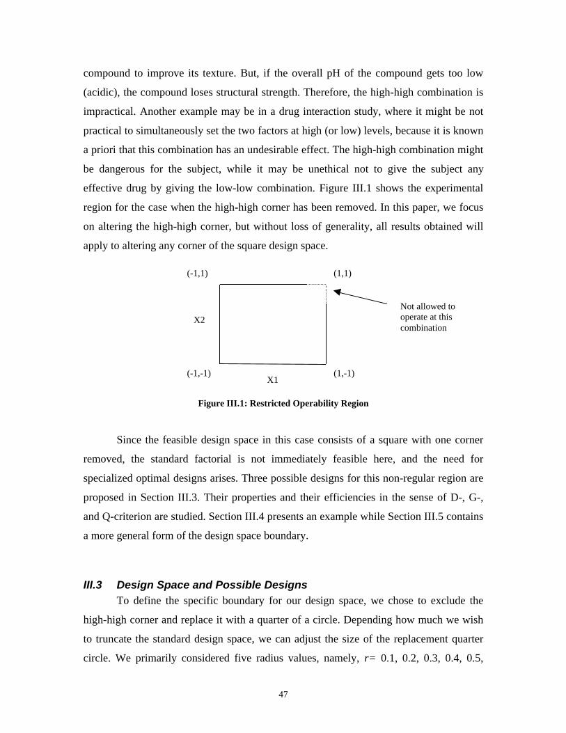
47
compound to improve its texture. But, if the overall pH of the compound gets too low
(acidic), the compound loses structural strength. Therefore, the high-high combination is
impractical. Another example may be in a drug interaction study, where it might be not
practical to simultaneously set the two factors at high (or low) levels, because it is known
a priori that this combination has an undesirable effect. The high-high combination might
be dangerous for the subject, while it may be unethical not to give the subject any
effective drug by giving the low-low combination. Figure III.1 shows the experimental
region for the case when the high-high corner has been removed. In this paper, we focus
on altering the high-high corner, but without loss of generality, all results obtained will
apply to altering any corner of the square design space.
Figure III.1: Restricted Operability Region
Since the feasible design space in this case consists of a square with one corner
removed, the standard factorial is not immediately feasible here, and the need for
specialized optimal designs arises. Three possible designs for this non-regular region are
proposed in Section III.3. Their properties and their efficiencies in the sense of D-, G-,
and Q-criterion are studied. Section III.4 presents an example while Section III.5 contains
a more general form of the design space boundary.
III.3 Design Space and Possible DesignsTo define the specific boundary for our design space, we chose to exclude the
high-high corner and replace it with a quarter of a circle. Depending how much we wish
to truncate the standard design space, we can adjust the size of the replacement quarter
circle. We primarily considered five radius values, namely, r= 0.1, 0.2, 0.3, 0.4, 0.5,
(1,1)(-1,1)
(1,-1)(-1,-1)X1
X2Not allowed tooperate at thiscombination
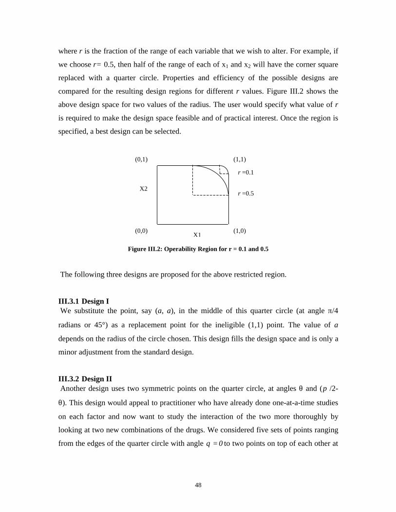
48
where r is the fraction of the range of each variable that we wish to alter. For example, if
we choose r= 0.5, then half of the range of each of x1 and x2 will have the corner square
replaced with a quarter circle. Properties and efficiency of the possible designs are
compared for the resulting design regions for different r values. Figure III.2 shows the
above design space for two values of the radius. The user would specify what value of r
is required to make the design space feasible and of practical interest. Once the region is
specified, a best design can be selected.
Figure III.2: Operability Region for r = 0.1 and 0.5
The following three designs are proposed for the above restricted region.
III.3.1 Design I We substitute the point, say (a, a), in the middle of this quarter circle (at angle π/4
radians or 45°) as a replacement point for the ineligible (1,1) point. The value of a
depends on the radius of the circle chosen. This design fills the design space and is only a
minor adjustment from the standard design.
III.3.2 Design II Another design uses two symmetric points on the quarter circle, at angles θ and (π /2-
θ). This design would appeal to practitioner who have already done one-at-a-time studies
on each factor and now want to study the interaction of the two more thoroughly by
looking at two new combinations of the drugs. We considered five sets of points ranging
from the edges of the quarter circle with angle 0=θ to two points on top of each other at
(1,1)(0,1)
(1,0)(0,0)X1
X2
r =0.1
r =0.5

49
the point (a, a) with 4/πθ = . This latter matches the design point of Design I, which
has just four design points whereas Design II has five points.
III.3.3 Design III If we wish to preserve an orthogonal design, we can use a standard factorial design in
the reduced space with the excluded high-high corner. This design might seem intuitively
pleasing to a practitioner who wishes to use a standard design and just changes the scale
of the coded variables to make it fit in the admissible region. The new cube region has the
points: (-1, -1), (-1, a), (a, -1), and (a, a), where a is the same point defined in Design I.
Although, the resulting design is orthogonal, it requires extrapolation to provide estimates
for the entire region. As the radius used for altering the design space increases, the
amount of extrapolation required will increase.
III.3.4 Comparison of DesignsTo select a single “best” design for this restricted region, there are several aspects
to consider. Properties of a good response surface design are discussed in Box and Hunter
(1957), Box and Draper (1975), Atkinson and Donev (1992) and Myers and Montgomery
(1995). Typically, one can not achieve all the ideal properties in a single design. Hence,
there are frequently several good designs and choosing among them involves some
tradeoffs. All of the designs above are able to estimate all of effects in the usual first
order model with interaction
εββββ ++++=211222110
xxxxy with ),0(N~ 2iid
σε .
To compare the three designs, we considered two sets of measures:
- Descriptive measures, which include number of design points, orthogonality,
how many levels per factor, ability to measure pure error.
- Quantitative measures including D-, G-, and Q-efficiency, maximum correlation
between any two parameter estimates, and the variance of the interaction term, which
may be of particular interest if the main effects are well understood.
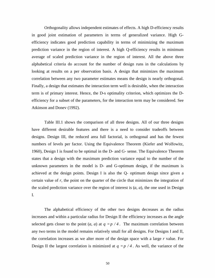
50
Orthogonality allows independent estimates of effects. A high D-efficiency results
in good joint estimation of parameters in terms of generalized variance. High G-
efficiency indicates good prediction capability in terms of minimizing the maximum
prediction variance in the region of interest. A high Q-efficiency results in minimum
average of scaled prediction variance in the region of interest. All the above three
alphabetical criteria do account for the number of design runs in the calculations by
looking at results on a per observation basis. A design that minimizes the maximum
correlation between any two parameter estimates means the design is nearly orthogonal.
Finally, a design that estimates the interaction term well is desirable, when the interaction
term is of primary interest. Hence, the D-s optimality criterion, which optimizes the D-
efficiency for a subset of the parameters, for the interaction term may be considered. See
Atkinson and Donev (1992).
Table III.1 shows the comparison of all three designs. All of our three designs
have different desirable features and there is a need to consider tradeoffs between
designs. Design III, the reduced area full factorial, is orthogonal and has the fewest
numbers of levels per factor. Using the Equivalence Theorem (Kiefer and Wolfowitz,
1960), Design I is found to be optimal in the D- and G- sense. The Equivalence Theorem
states that a design with the maximum prediction variance equal to the number of the
unknown parameters in the model is D- and G-optimum design, if the maximum is
achieved at the design points. Design I is also the Q- optimum design since given a
certain value of r, the point on the quarter of the circle that minimizes the integration of
the scaled prediction variance over the region of interest is (a, a), the one used in Design
I.
The alphabetical efficiency of the other two designs decreases as the radius
increases and within a particular radius for Design II the efficiency increases as the angle
selected gets closer to the point (a, a) at 4/πθ = . The maximum correlation between
any two terms in the model remains relatively small for all designs. For Designs I and II,
the correlation increases as we alter more of the design space with a large r value. For
Design II the largest correlation is minimized at 4/πθ = . As well, the variance of the
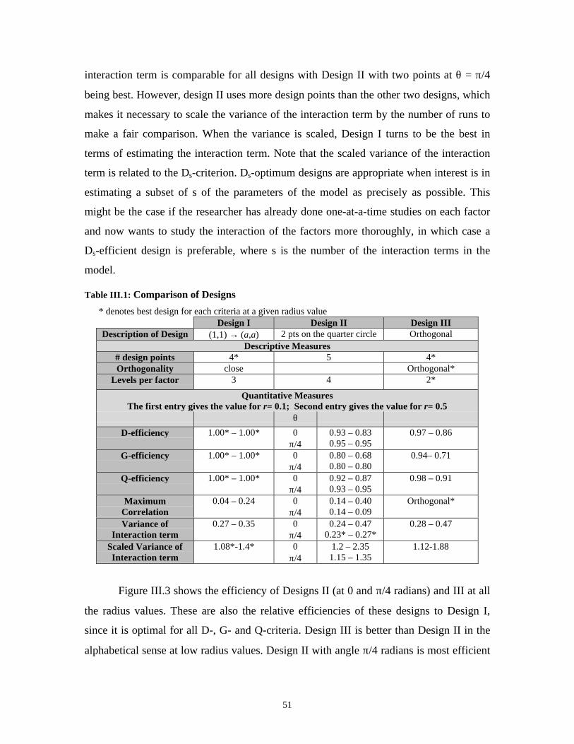
51
interaction term is comparable for all designs with Design II with two points at θ = π/4
being best. However, design II uses more design points than the other two designs, which
makes it necessary to scale the variance of the interaction term by the number of runs to
make a fair comparison. When the variance is scaled, Design I turns to be the best in
terms of estimating the interaction term. Note that the scaled variance of the interaction
term is related to the Ds-criterion. Ds-optimum designs are appropriate when interest is in
estimating a subset of s of the parameters of the model as precisely as possible. This
might be the case if the researcher has already done one-at-a-time studies on each factor
and now wants to study the interaction of the factors more thoroughly, in which case a
Ds-efficient design is preferable, where s is the number of the interaction terms in the
model.
Table III.1: Comparison of Designs
* denotes best design for each criteria at a given radius valueDesign I Design II Design III
Description of Design (1,1) → (a,a) 2 pts on the quarter circle OrthogonalDescriptive Measures
# design points 4* 5 4*Orthogonality close Orthogonal*
Levels per factor 3 4 2*
Quantitative MeasuresThe first entry gives the value for r= 0.1; Second entry gives the value for r= 0.5
θ
D-efficiency 1.00* – 1.00* 0π/4
0.93 – 0.830.95 – 0.95
0.97 – 0.86
G-efficiency 1.00* – 1.00* 0π/4
0.80 – 0.680.80 – 0.80
0.94– 0.71
Q-efficiency 1.00* – 1.00* 0π/4
0.92 – 0.870.93 – 0.95
0.98 – 0.91
MaximumCorrelation
0.04 – 0.24 0π/4
0.14 – 0.400.14 – 0.09
Orthogonal*
Variance ofInteraction term
0.27 – 0.35 0π/4
0.24 – 0.470.23* – 0.27*
0.28 – 0.47
Scaled Variance ofInteraction term
1.08*-1.4* 0π/4
1.2 – 2.351.15 – 1.35
1.12-1.88
Figure III.3 shows the efficiency of Designs II (at 0 and π/4 radians) and III at all
the radius values. These are also the relative efficiencies of these designs to Design I,
since it is optimal for all D-, G- and Q-criteria. Design III is better than Design II in the
alphabetical sense at low radius values. Design II with angle π/4 radians is most efficient
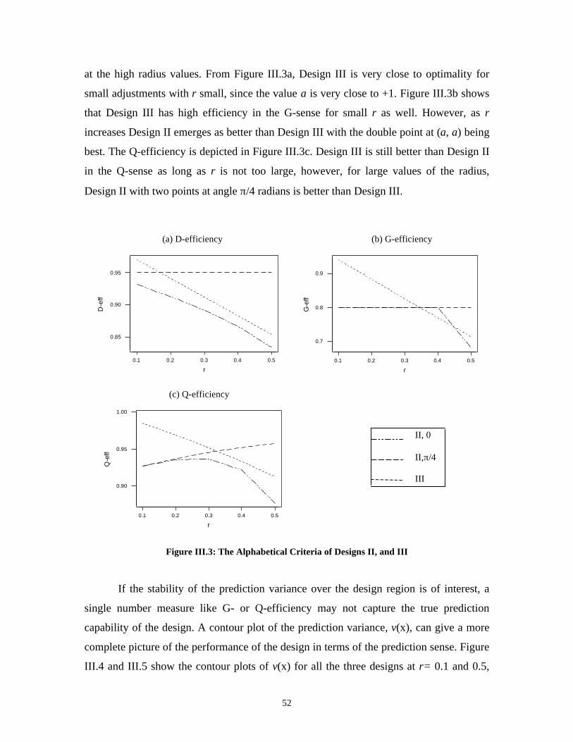
52
at the high radius values. From Figure III.3a, Design III is very close to optimality for
small adjustments with r small, since the value a is very close to +1. Figure III.3b shows
that Design III has high efficiency in the G-sense for small r as well. However, as r
increases Design II emerges as better than Design III with the double point at (a, a) being
best. The Q-efficiency is depicted in Figure III.3c. Design III is still better than Design II
in the Q-sense as long as r is not too large, however, for large values of the radius,
Design II with two points at angle π/4 radians is better than Design III.
Figure III.3: The Alphabetical Criteria of Designs II, and III
If the stability of the prediction variance over the design region is of interest, a
single number measure like G- or Q-efficiency may not capture the true prediction
capability of the design. A contour plot of the prediction variance, v(x), can give a more
complete picture of the performance of the design in terms of the prediction sense. Figure
III.4 and III.5 show the contour plots of v(x) for all the three designs at r= 0.1 and 0.5,
0.1 0.2 0.3 0.4 0.5
0.85
0.90
0.95
r
D-e
ff
II, 0
II,π/4
III
0.1 0.2 0.3 0.4 0.5
0.90
0.95
1.00
r
Q-e
ff
0.50.40.30.20.1
0.9
0.8
0.7
r
G-e
ff
(a) D-efficiency (b) G-efficiency
(c) Q-efficiency
53
respectively. For small adjustments to the region ( 1.0r = ) in Figure III.4, Design I is
nearly rotatable. The effect of excluding the high-high corner results in having a slightly
higher prediction variance than any other corner. Design III is rotatable, while Design II
is the least rotatable. Since Design I is optimal in both G- and Q-sense, it has the smallest
levels of prediction variance contours in the region of interest. However, if the researcher
is primarily interested in the adjusted corner, Design II performs best. Figure III.5 shows
that Design II with angle π/4 radians has the lowest values of the prediction variance at
the adjusted corner, which helps it in the Q-sense. For large radii, Design III loses its
good Q-efficiency because of the large region with extrapolation and high prediction
variances.
Figure III.4: Contour Plots of v(x) for the three Designs at r=0.1
All of the above designs, of course, can accommodate center runs. As with the
standard designs, the effect of center runs result in the alphabet optimality efficiencies
10-1
1
0
-1
x1
x2
Design I
-1 0 1
-1
0
1
x1
Design II ,
x2
-1 0 1
-1
0
1
x1
x2
Design III
1.5
2.0
3.0
4.0
5.0
6.0
7.0
θ=π/4
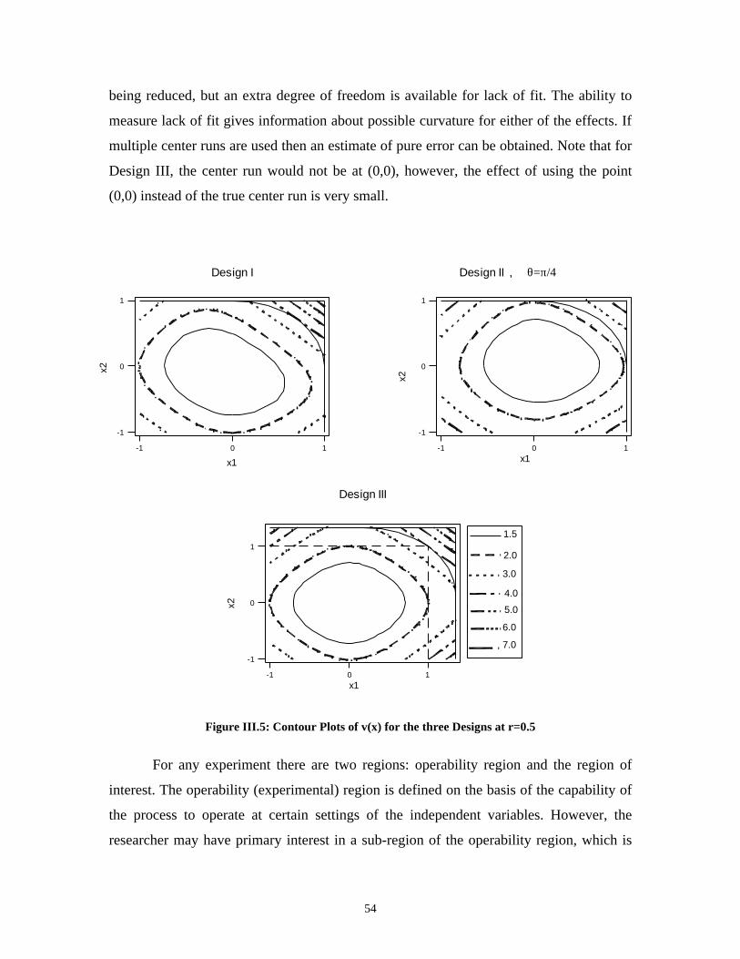
54
being reduced, but an extra degree of freedom is available for lack of fit. The ability to
measure lack of fit gives information about possible curvature for either of the effects. If
multiple center runs are used then an estimate of pure error can be obtained. Note that for
Design III, the center run would not be at (0,0), however, the effect of using the point
(0,0) instead of the true center run is very small.
Figure III.5: Contour Plots of v(x) for the three Designs at r=0.5
For any experiment there are two regions: operability region and the region of
interest. The operability (experimental) region is defined on the basis of the capability of
the process to operate at certain settings of the independent variables. However, the
researcher may have primary interest in a sub-region of the operability region, which is
-1 0 1
-1
0
1
x1
x2
Design III
1.5
2.0
3.0
4.0
5.0
6.0
7.0
-1 0 1
-1
0
1
x1
x2
Design II ,
10-1
1
0
-1
x1
x2
Design I θ=π/4
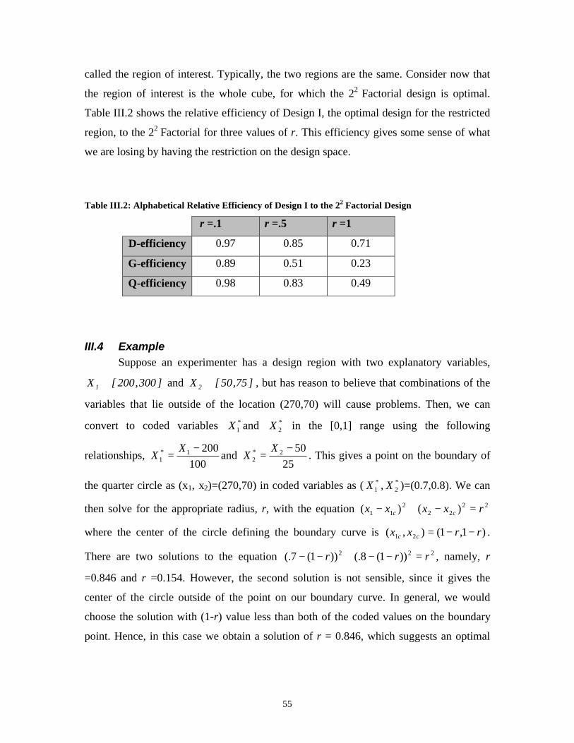
55
called the region of interest. Typically, the two regions are the same. Consider now that
the region of interest is the whole cube, for which the 22 Factorial design is optimal.
Table III.2 shows the relative efficiency of Design I, the optimal design for the restricted
region, to the 22 Factorial for three values of r. This efficiency gives some sense of what
we are losing by having the restriction on the design space.
Table III.2: Alphabetical Relative Efficiency of Design I to the 22 Factorial Design
r =.1 r =.5 r =1
D-efficiency 0.97 0.85 0.71
G-efficiency 0.89 0.51 0.23
Q-efficiency 0.98 0.83 0.49
III.4 ExampleSuppose an experimenter has a design region with two explanatory variables,
]300 ,200[X 1 ∈ and ]57 ,50[X 2 ∈ , but has reason to believe that combinations of the
variables that lie outside of the location (270,70) will cause problems. Then, we can
convert to coded variables *1X and *
2X in the [0,1] range using the following
relationships, 100
2001*1
−=
XX and
25502*
2
−=
XX . This gives a point on the boundary of
the quarter circle as (x1, x2)=(270,70) in coded variables as ( *1X , *
2X )=(0.7,0.8). We can
then solve for the appropriate radius, r, with the equation 2222
211 )()( rxxxx cc =−+−
where the center of the circle defining the boundary curve is )1,1(),( 21 rrxx cc −−= .
There are two solutions to the equation 222 ))1(8(.))1(7(. rrr =−−+−− , namely, r
=0.846 and r =0.154. However, the second solution is not sensible, since it gives the
center of the circle outside of the point on our boundary curve. In general, we would
choose the solution with (1-r) value less than both of the coded values on the boundary
point. Hence, in this case we obtain a solution of r = 0.846, which suggests an optimal

56
design point using Design I in the restricted region of )752,.752(.)1,1(22
=+−+− rr rr
in coded variables or (275.2, 68.8) in the original variables.
If it were not possible to run the experiment with these precise values at these
experimental conditions, but instead needed to round to the nearest unit, then it would be
necessary to round down for both variables to ensure that we remain in the feasible
region. This would yield the location of (275, 68) in the restricted corner, as well as the
standard design points of (200,50), (200, 75), (300, 50) in the other corners of the design
space. However, this rounding results in a different design than Design I. If one would
like to use the optimal design (Design I), then it is better to round down the radius value
or to change the coded values a little bit. In our case, one could use (0.76,0.76) which is
(276,69) in the original scale and has a radius value of 0.819.
III.5 General Design Space and Design IThe optimality of Design I in the sense of all three alphabetical criteria
encourages us to check its optimality for other related design spaces. So far, we
considered replacing the high-high corner of the cube with a quarter of a circle of radius
r, i.e., we implemented the equation 2222
211 )()( rxxxx cc =−+− , where (x1c, x2c) = (1-
r,1-r) the center of our circle. A more general equation that gives flexibility of the design
space is ddc
dc rxxxx =−+− |||| 2211 , for d > 0. Figure III.6 shows the effect of
changing the value of d on the design space. For d=1 we have a straight line truncating
the corner. To make the design space as close as possible to the cuboidal standard design
space, we could use increasing powers of d. This is beneficial only if the interaction
between the two factors is known a priori to be positive, or synergistic. However, if the
interaction between the two factors is known to be negative it may be more appropriate to
use a d value less than 1.
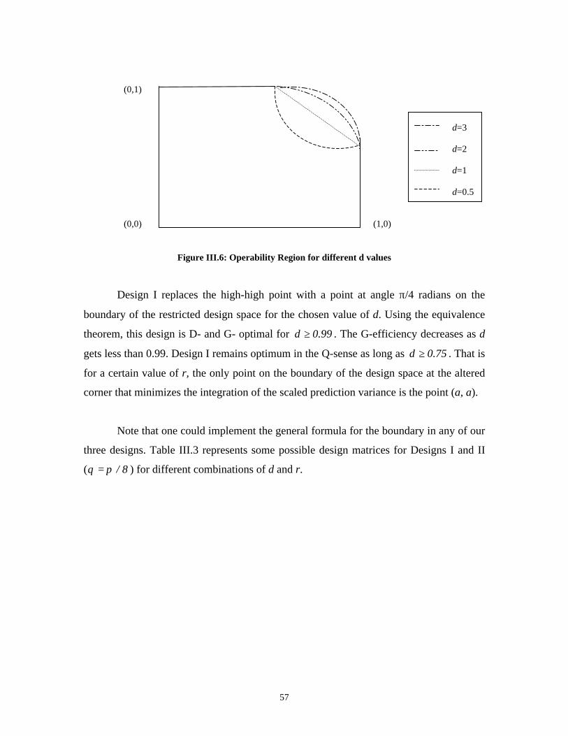
57
Figure III.6: Operability Region for different d values
Design I replaces the high-high point with a point at angle π/4 radians on the
boundary of the restricted design space for the chosen value of d. Using the equivalence
theorem, this design is D- and G- optimal for 99.0d ≥ . The G-efficiency decreases as d
gets less than 0.99. Design I remains optimum in the Q-sense as long as 75.0d ≥ . That is
for a certain value of r, the only point on the boundary of the design space at the altered
corner that minimizes the integration of the scaled prediction variance is the point (a, a).
Note that one could implement the general formula for the boundary in any of our
three designs. Table III.3 represents some possible design matrices for Designs I and II
( 8/πθ = ) for different combinations of d and r.
(0,1)
(1,0)(0,0)
d=3
d=2
d=1
d=0.5
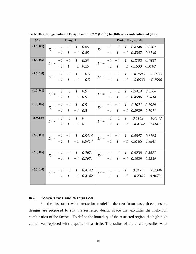
58
Table III.3: Design matrix of Design I and II ( 8/πθ = ) for Different combinations of (d, r)
(d, r) Design I Design II (θ = π /8)
(0.5, 0.1)
−−
−−=′
85.011185.0111
D
−−
−−=′
8740.08307.01118307.08740.0111
D
(0.5, 0.5)
−−
−−=′
25.011125.0111
D
−−
−−=′
3702.01533.01111533.03702.0111
D
(0.5, 1.0)
−−−−−−
=′5.01115.0111
D
−−−−−−−−
=′2596.06933.01116933.02596.0111
D
(1.0, 0.1)
−−
−−=′
9.01119.0111
D
−−
−−=′
9414.08586.01118586.09414.0111
D
(1.0, 0.5)
−−
−−=′
5.01115.0111
D
−−
−−=′
7071.02929.01112929.07071.0111
D
(1.0,1.0)
−−
−−=′
01110111
D
−−−
−−−=′
4142.04142.01114142.04142.0111
D
(2.0, 0.1)
−−
−−=′
9414.01119414.0111
D
−−
−−=′
9847.08765.01118765.09847.0111
D
(2.0, 0.5)
−−
−−=′
7071.01117071.0111
D
−−
−−=′
9239.03829.01113827.09239.0111
D
(2.0, 1.0)
−−
−−=′
4142.01114142.0111
D
−−−
−−−=′
8478.02346.01112346.08478.0111
D
III.6 Conclusions and DiscussionFor the first order with interaction model in the two-factor case, three sensible
designs are proposed to suit the restricted design space that excludes the high-high
combination of the factors. To define the boundary of the restricted region, the high-high
corner was replaced with a quarter of a circle. The radius of the circle specifies what
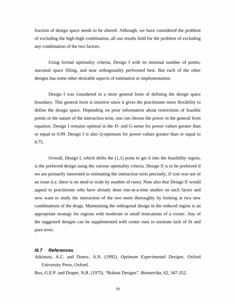
59
fraction of design space needs to be altered. Although, we have considered the problem
of excluding the high-high combination, all our results hold for the problem of excluding
any combination of the two factors.
Using formal optimality criteria, Design I with its minimal number of points,
maximal space filling, and near orthogonality performed best. But each of the other
designs has some other desirable aspects of estimation or implementation.
Design I was considered in a more general form of defining the design space
boundary. This general form is intuitive since it gives the practitioner more flexibility to
define the design space. Depending on prior information about restrictions of feasible
points or the nature of the interaction term, one can choose the power in the general form
equation. Design I remains optimal in the D- and G-sense for power values greater than
or equal to 0.99. Design I is also Q-optimum for power values greater than or equal to
0.75.
Overall, Design I, which shifts the (1,1) point to get it into the feasibility region,
is the preferred design using the various optimality criteria. Design II is to be preferred if
we are primarily interested in estimating the interaction term precisely, if cost was not of
an issue (i.e. there is no need to scale by number of runs). Note also that Design II would
appeal to practitioner who have already done one-at-a-time studies on each factor and
now want to study the interaction of the two more thoroughly by looking at two new
combinations of the drugs. Maintaining the orthogonal design in the reduced region is an
appropriate strategy for regions with moderate or small truncations of a corner. Any of
the suggested designs can be supplemented with center runs to estimate lack of fit and
pure error.
III.7 ReferencesAtkinson, A.C. and Donev, A.N. (1992). Optimum Experimental Designs. Oxford
University Press, Oxford.
Box, G.E.P. and Draper, N.R. (1975). “Robust Designs”. Biometrika, 62, 347-352.
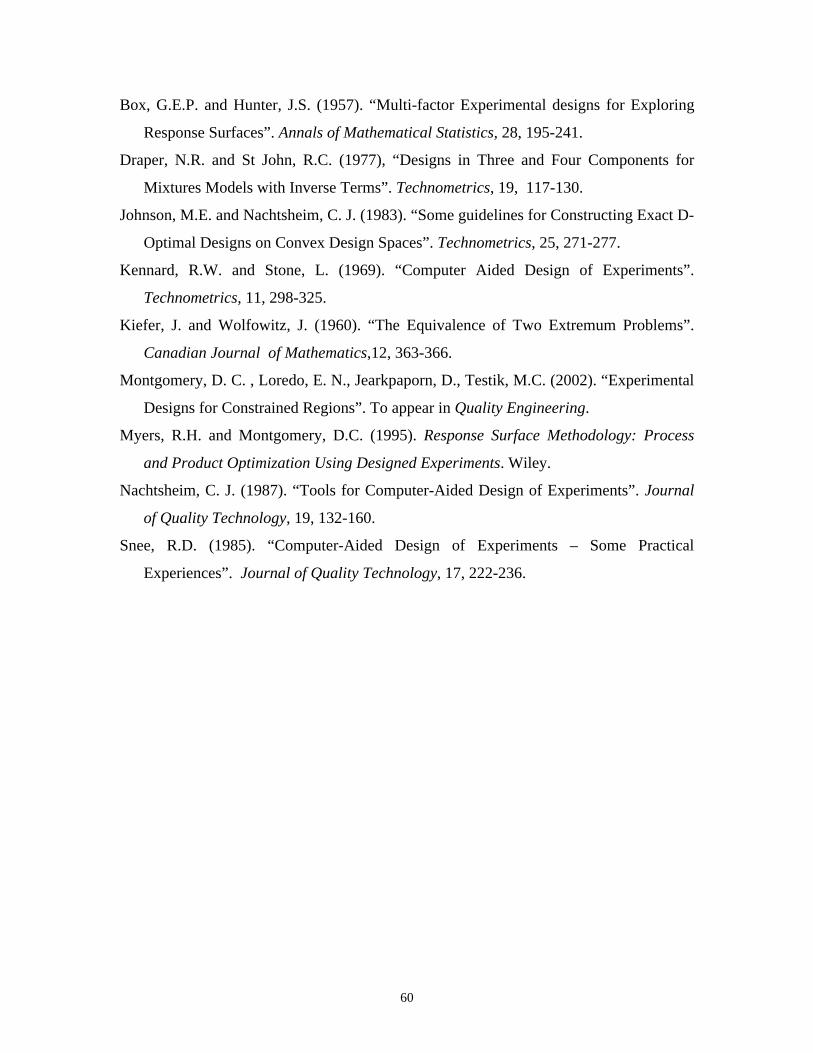
60
Box, G.E.P. and Hunter, J.S. (1957). “Multi-factor Experimental designs for Exploring
Response Surfaces”. Annals of Mathematical Statistics, 28, 195-241.
Draper, N.R. and St John, R.C. (1977), “Designs in Three and Four Components for
Mixtures Models with Inverse Terms”. Technometrics, 19, 117-130.
Johnson, M.E. and Nachtsheim, C. J. (1983). “Some guidelines for Constructing Exact D-
Optimal Designs on Convex Design Spaces”. Technometrics, 25, 271-277.
Kennard, R.W. and Stone, L. (1969). “Computer Aided Design of Experiments”.
Technometrics, 11, 298-325.
Kiefer, J. and Wolfowitz, J. (1960). “The Equivalence of Two Extremum Problems”.
Canadian Journal of Mathematics,12, 363-366.
Montgomery, D. C. , Loredo, E. N., Jearkpaporn, D., Testik, M.C. (2002). “Experimental
Designs for Constrained Regions”. To appear in Quality Engineering.
Myers, R.H. and Montgomery, D.C. (1995). Response Surface Methodology: Process
and Product Optimization Using Designed Experiments. Wiley.
Nachtsheim, C. J. (1987). “Tools for Computer-Aided Design of Experiments”. Journal
of Quality Technology, 19, 132-160.
Snee, R.D. (1985). “Computer-Aided Design of Experiments – Some Practical
Experiences”. Journal of Quality Technology, 17, 222-236.

61
Supplement I: Modifying 23 Factorial to Accommodate a Restricted DesignSpace
In this section, we generalize the three designs (I, II, III) presented in Chapter III
to the three-factor setup. For the quantitative three-factor case the standard cuboidal
experimental region is the cube. Consider for some reason the high-high-high (H-H-H)
combination of the factors is prohibited. Analogous to the previous chapter, we chose to
exclude a cube of side length r from the restricted H-H-H corner and replace it with a
sector of a sphere of radius 2r=ρ centered at )r1 ,r1 ,r1( −−− . Figure SI.1
represents the operability region in this case. The total volume of this restricted design
space in the [0,1]2 scale is calculated as follows
)1( 31
1
1
1
1
1123 rdxdxdxwvolume
r r r
−+= ∫ ∫ ∫− − −
where ε+
+=
g
ggw
21
, ε is a small number used to ensure that the denominator is greater
than zero and ∑=
−−−=r
ii rxg
1
22 ))1((ρ . The function w is an indicator function to filter
out the points outside the sphere in the restricted corner.
Design I replaces the H-H-H point in [0,1]2 scale with the point
)a,a,a(a* = where 3/r1a ρ+−= . Design II uses three points to replace the H-H-H
point: )x,x,x(a i3i2i1*i = , where )r1(sinsinx iii1 −+= θφρ ,
)r1(cossinx iii2 −+= θφρ and )r1(cos x ii3 −+= φρ , i=1,2,3. The angles (θi , φi) are
defined in Figure SI.2. We considered two sets of the angles [(θ1, φ1), (θ2, φ2), (θ3, φ3)].
Set 1 is )]90,45(),45,0(),45,90[( °°°°°° , this set gives us three edge-points: (1-r, 1, 1),
(1,1-r,1), (1, 1,1-r), respectively, corresponding to the angle value o0 in the two-factor
case. Set 2 is °=°= 7356.54,45 ii φθ , i=1,2,3, which results in three points on top of
each other corresponding to the angle value o45 in the two-factor case and the point
)a,a,a(a* = of Design I. Design III uses the same point a* of Design I, but it also

62
modifies all the other corners that include the high level. The design matrix in [-1,1]2
scale is as following
−−
−−−
−−−−
−−−
=
bbbbb
bbb
bbb
b
xxx
DIII
11
111
1111
111321
where b is the corresponding value of a in the [-1,1] scale. Note that Design III is just a
smaller regular factorial, which does not fill the whole experimental space shown in
Figure SI.1. An extrapolation space of [volume-a3] is present in the [0,1]2 scale. Figure
SI.3 shows the total volume of the experimental region and the volume of the cube
implemented in Design III (a3). The figure shows how the extrapolation area increases
rapidly as r increases while the volume of the experimental decreases slowly.
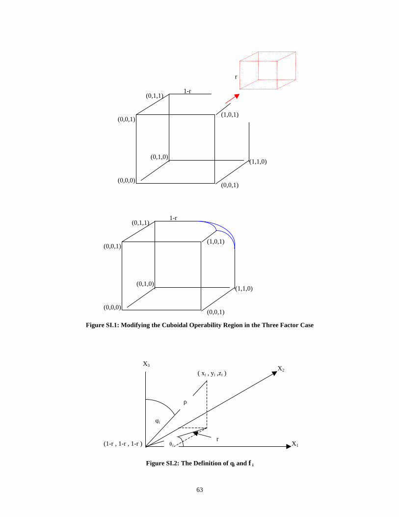
63
Figure SI.1: Modifying the Cuboidal Operability Region in the Three Factor Case
Figure SI.2: The Definition of θi and φi
(1-r , 1-r , 1-r )
X2
rX1
( xi , yi ,zi )
φi
θi
ρ
X3
(0,1,0)
(0,1,0)
r
(1,1,0)
(0,0,1)(0,0,0)
(0,1,1)1-r
(0,0,1)(1,0,1)
(1,1,0)
(0,0,1)(0,0,0)
(0,1,1)1-r
(0,0,1)(1,0,1)
64
0 0.2 0.4 0.6 0.8 1r
0.4
0.6
0.8
1
Volu
me
Experimental Region
Design III Region
Figure SI.3: Total Space Volume of the Restricted Region and the Volume of the Design Space ofDesign III
We will discuss two first order models with interaction in the three-factor case:
Model I considers only the main effects with two-way interactions (without the three-way
interaction term) while Model II contains main effects and all possible interactions (two-
and three-way interactions). Equations SI.1 and SI.2 show the functional forms of Model
I and Model II, respectively.
∑∑∑<=
++=33
10
jijiij
iii xxxy βββ (SI.1)
321123
33
10 xxxxxxy
jijiij
iii ββββ +++= ∑∑∑
<=
(SI.2)
Model I would be the more common choice in response surface modeling, but there may
be situations when we wish to consider a three-way interaction term in the model. Design
I with Model II is saturated and is the D- and G-optimum design for our restricted region.

65
For Model I, Table SI.1 compares the three designs in terms of the descriptive
and quantitative measures, discussed in the two-factor case. Design III, the reduced area
full factorial, is orthogonal and has the fewest numbers of levels per factor. Design I has
the highest determinant of the information matrix and the lowest SPV among the three
designs. Therefore, its D- and Q- efficiency in Table SI.1 is set to one and the relative D-
and Q-efficiency of the other two designs relative to Design I is calculated. Table SI.1
shows the G-efficiency of all the designs relative to the G-optimum design, which by
theorem has maximum scaled prediction variance equal to P. Design I is the most G-
efficient design. Note that the same behavior of the Q-efficiency of Design II here is as it
was in the two factor case, namely an increasing function in the side length of the
excluded cube. In general, the alphabetical efficiency decreases as the side length of the
excluded cube, r, increases and within a particular value of r for Design II the efficiency
increases as the three points gets closer to the point a*. The maximum correlation
between any two terms in the model remains relatively small for all designs. For Designs
I and II, the correlation increases as we alter more of the design space with a large r
value. For Design II the largest correlation between any two terms in the model is
minimized with Set 2, the three points at a*. Design I also is the most Ds-efficient design.
Ds-optimum designs are appropriate when interest is in estimating a subset of s of the
parameters of the model as precisely as possible. This might be the case if the researcher
has already done one-at-a-time studies on each factor and now wants to study the
interaction of the factors more thoroughly, in which case a Ds-efficient design is
preferable, where s is the number of the interaction terms in the model. The Ds-optimum
design is that design that maximizes 22
111 );(
M
XMM
β=
−, where the moment matrix is
partitioned as
′
==2212
1211);(1
);(MMMM
XIN
XM ββ and M11, the s×s left upper sub-
matrix of ),(1 XM β− , is the covariance matrix for the least squares estimates of the s
parameters we are interested in (Atkinson and Donev, 1992). Table SI.1 shows the Ds-
efficiency of Design II and III relative to Design I . Design III is the second best design in
terms of the Ds-sense for small values of r, but it is the worst design for large values of r.
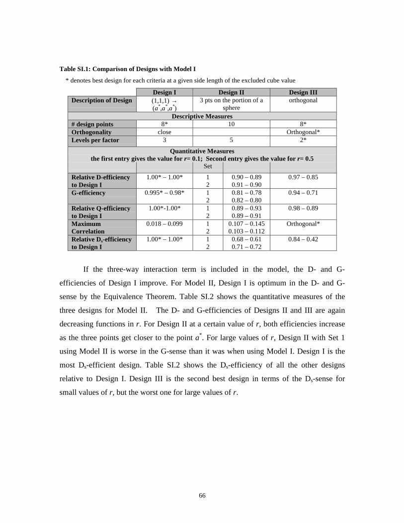
66
Table SI.1: Comparison of Designs with Model I
* denotes best design for each criteria at a given side length of the excluded cube value
Design I Design II Design IIIDescription of Design (1,1,1) →
(a*,a*,a*)3 pts on the portion of a
sphereorthogonal
Descriptive Measures# design points 8* 10 8*Orthogonality close Orthogonal*Levels per factor 3 5 2*
Quantitative Measuresthe first entry gives the value for r= 0.1; Second entry gives the value for r= 0.5
Set
Relative D-efficiencyto Design I
1.00* – 1.00* 12
0.90 – 0.890.91 – 0.90
0.97 – 0.85
G-efficiency 0.995* – 0.98* 12
0.81 – 0.780.82 – 0.80
0.94 – 0.71
Relative Q-efficiencyto Design I
1.00*-1.00* 12
0.89 – 0.930.89 – 0.91
0.98 – 0.89
MaximumCorrelation
0.018 – 0.099 12
0.107 – 0.1450.103 – 0.112
Orthogonal*
Relative Ds-efficiencyto Design I
1.00* – 1.00* 12
0.68 – 0.610.71 – 0.72
0.84 – 0.42
If the three-way interaction term is included in the model, the D- and G-
efficiencies of Design I improve. For Model II, Design I is optimum in the D- and G-
sense by the Equivalence Theorem. Table SI.2 shows the quantitative measures of the
three designs for Model II. The D- and G-efficiencies of Designs II and III are again
decreasing functions in r. For Design II at a certain value of r, both efficiencies increase
as the three points get closer to the point a*. For large values of r, Design II with Set 1
using Model II is worse in the G-sense than it was when using Model I. Design I is the
most Ds-efficient design. Table SI.2 shows the Ds-efficiency of all the other designs
relative to Design I. Design III is the second best design in terms of the Ds-sense for
small values of r, but the worst one for large values of r.
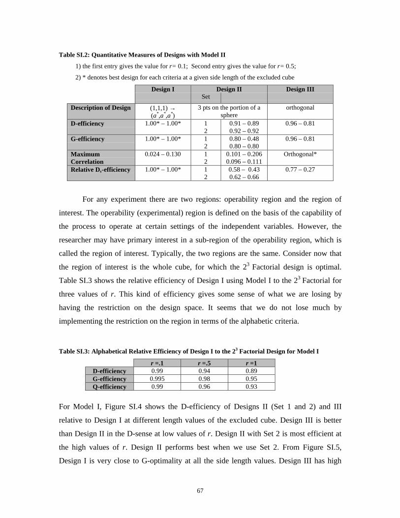
67
Table SI.2: Quantitative Measures of Designs with Model II
1) the first entry gives the value for r= 0.1; Second entry gives the value for r= 0.5;
2) * denotes best design for each criteria at a given side length of the excluded cube
Design I Design II Design IIISet
Description of Design (1,1,1) →(a*,a*,a*)
3 pts on the portion of asphere
orthogonal
D-efficiency 1.00* – 1.00* 12
0.91 – 0.890.92 – 0.92
0.96 – 0.81
G-efficiency 1.00* – 1.00* 12
0.80 – 0.480.80 – 0.80
0.96 – 0.81
MaximumCorrelation
0.024 – 0.130 12
0.101 – 0.2060.096 – 0.111
Orthogonal*
Relative Ds-efficiency 1.00* – 1.00* 12
0.58 – 0.430.62 – 0.66
0.77 – 0.27
For any experiment there are two regions: operability region and the region of
interest. The operability (experimental) region is defined on the basis of the capability of
the process to operate at certain settings of the independent variables. However, the
researcher may have primary interest in a sub-region of the operability region, which is
called the region of interest. Typically, the two regions are the same. Consider now that
the region of interest is the whole cube, for which the 23 Factorial design is optimal.
Table SI.3 shows the relative efficiency of Design I using Model I to the 23 Factorial for
three values of r. This kind of efficiency gives some sense of what we are losing by
having the restriction on the design space. It seems that we do not lose much by
implementing the restriction on the region in terms of the alphabetic criteria.
Table SI.3: Alphabetical Relative Efficiency of Design I to the 23 Factorial Design for Model I
r =.1 r =.5 r =1D-efficiency 0.99 0.94 0.89G-efficiency 0.995 0.98 0.95Q-efficiency 0.99 0.96 0.93
For Model I, Figure SI.4 shows the D-efficiency of Designs II (Set 1 and 2) and III
relative to Design I at different length values of the excluded cube. Design III is better
than Design II in the D-sense at low values of r. Design II with Set 2 is most efficient at
the high values of r. Design II performs best when we use Set 2. From Figure SI.5,
Design I is very close to G-optimality at all the side length values. Design III has high
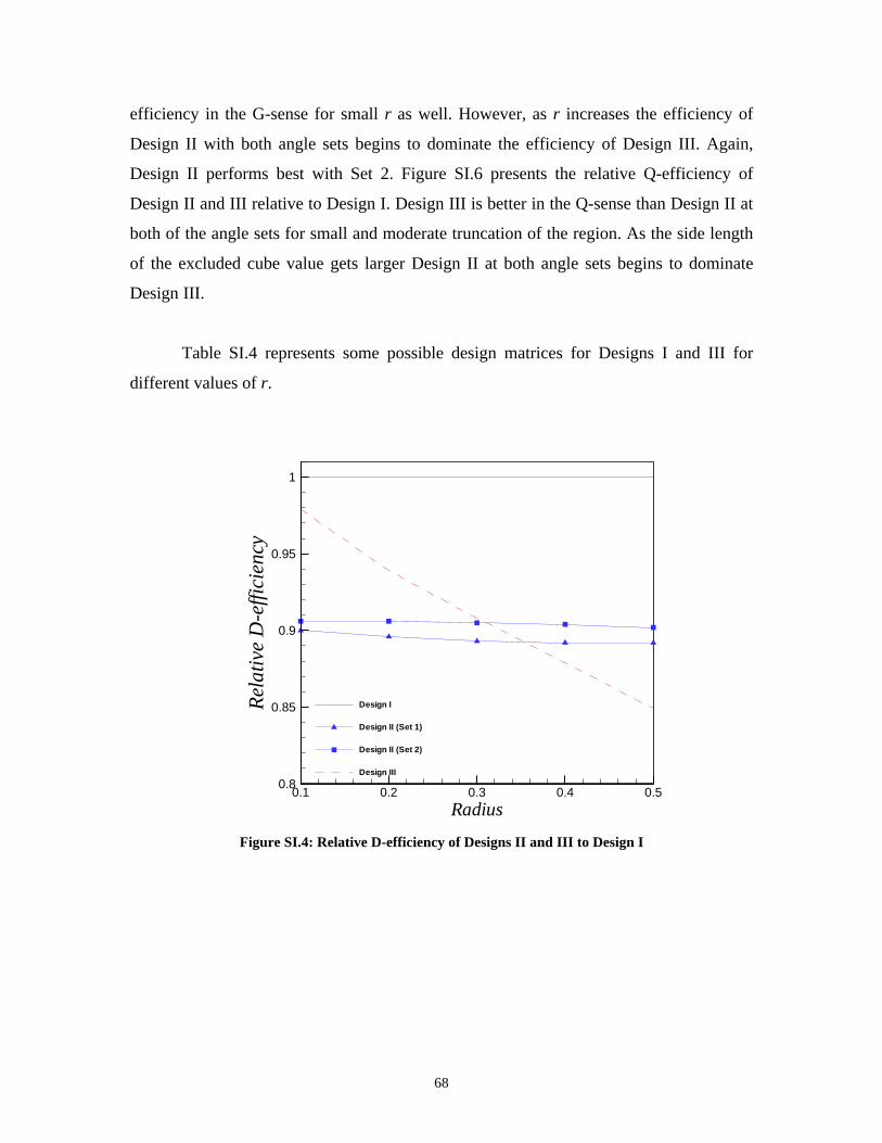
68
efficiency in the G-sense for small r as well. However, as r increases the efficiency of
Design II with both angle sets begins to dominate the efficiency of Design III. Again,
Design II performs best with Set 2. Figure SI.6 presents the relative Q-efficiency of
Design II and III relative to Design I. Design III is better in the Q-sense than Design II at
both of the angle sets for small and moderate truncation of the region. As the side length
of the excluded cube value gets larger Design II at both angle sets begins to dominate
Design III.
Table SI.4 represents some possible design matrices for Designs I and III for
different values of r.
Figure SI.4: Relative D-efficiency of Designs II and III to Design I
0.1 0.2 0.3 0.4 0.5Radius
0.8
0.85
0.9
0.95
1
Rela
tive
D-e
ffici
ency
Design I
Design II (Set 1)
Design II (Set 2)
Design III
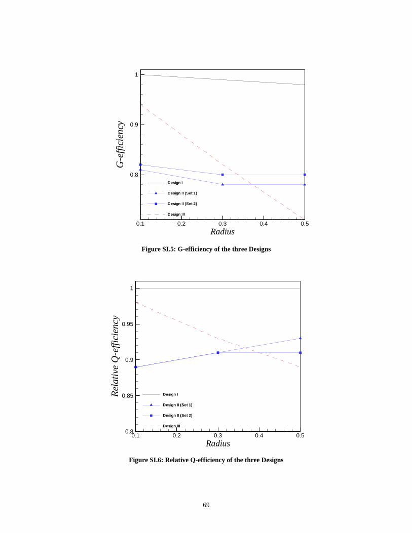
69
Figure SI.5: G-efficiency of the three Designs
Figure SI.6: Relative Q-efficiency of the three Designs
0.1 0.2 0.3 0.4 0.5Radius
0.8
0.85
0.9
0.95
1
Rela
tive
Q-e
ffici
ency
Design I
Design II (Set 1)
Design II (Set 2)
Design III
0.1 0.2 0.3 0.4 0.5Radius
0.8
0.9
1
G-e
ffici
ency
Design I
Design II (Set 1)
Design II (Set 2)
Design III
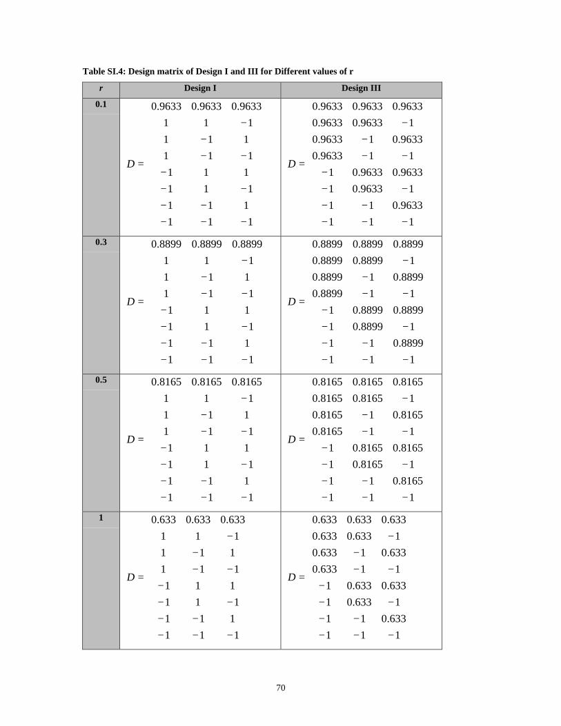
70
Table SI.4: Design matrix of Design I and III for Different values of r
r Design I Design III
0.1
−−−−−
−−−
−−−
−
=
111111111
111111
111111
9633.09633.09633.0
D
−−−−−
−−−
−−−
−
=
1119633.011
19633.019633.09633.01
119633.09633.019633.0
19633.09633.09633.09633.09633.0
D
0.3
−−−−−
−−−
−−−
−
=
111111111
111111
111111
0.88990.88990.8899
D
−−−−−
−−−
−−−
−
=
1110.889911
10.889910.88990.88991
110.88990.889910.8899
10.88990.88990.88990.88990.8899
D
0.5
−−−−−
−−−
−−−
−
=
111111111
111111
111111
0.81650.81650.8165
D
−−−−−
−−−
−−−
−
=
1110.816511
10.816510.81650.81651
110.81650.816510.8165
10.81650.81650.81650.81650.8165
D
1
−−−−−
−−−
−−−
−
=
111111111
111111
111111
0.6330.6330.633
D
−−−−−
−−−
−−−
−
=
1110.63311
10.63310.6330.6331
110.6330.63310.633
10.6330.6330.6330.6330.633
D
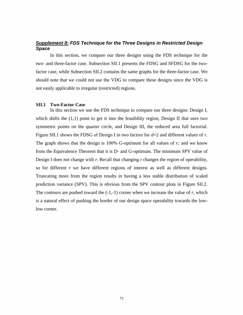
71
Supplement II: FDS Technique for the Three Designs in Restricted DesignSpace
In this section, we compare our three designs using the FDS technique for the
two- and three-factor case. Subsection SII.1 presents the FDSG and SFDSG for the two-
factor case, while Subsection SII.2 contains the same graphs for the three-factor case. We
should note that we could not use the VDG to compare these designs since the VDG is
not easily applicable to irregular (restricted) regions.
SII.1 Two-Factor CaseIn this section we use the FDS technique to compare our three designs: Design I,
which shifts the (1,1) point to get it into the feasibility region, Design II that uses two
symmetric points on the quarter circle, and Design III, the reduced area full factorial.
Figure SII.1 shows the FDSG of Design I in two factors for d=2 and different values of r.
The graph shows that the design is 100% G-optimum for all values of r; and we know
from the Equivalence Theorem that it is D- and G-optimum. The minimum SPV value of
Design I does not change with r. Recall that changing r changes the region of operability,
so for different r we have different regions of interest as well as different designs.
Truncating more from the region results in having a less stable distribution of scaled
prediction variance (SPV). This is obvious from the SPV contour plots in Figure SII.2.
The contours are pushed toward the (-1,-1) corner when we increase the value of r, which
is a natural effect of pushing the border of our design space operability towards the low-
low corner.
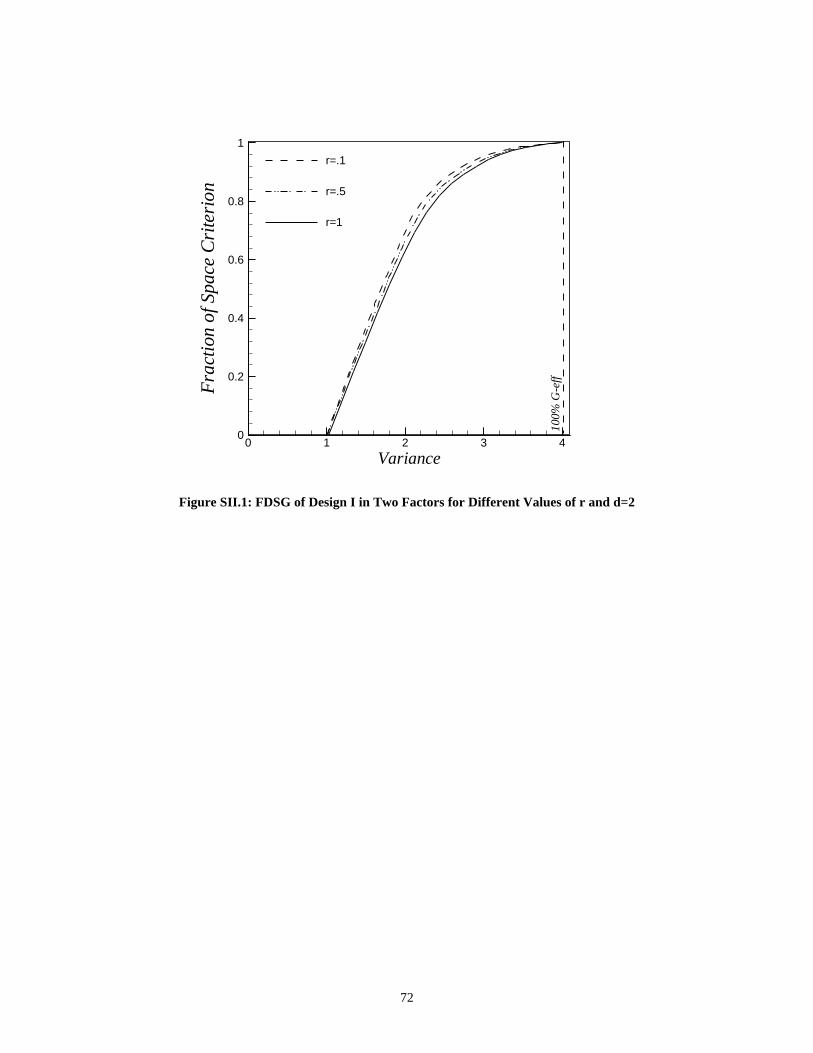
72
0 1 2 3 4Variance
0
0.2
0.4
0.6
0.8
1
Frac
tion
ofSp
ace
Cri
teri
on
r=.1
r=.5
r=1
100%
G-e
ff
Figure SII.1: FDSG of Design I in Two Factors for Different Values of r and d=2
73
Figure SII.2: Contour Plots of v(x) for Design I at r=0.1, 0.5, 1
Figure SII.3 presents the FDSG of Design I, II ( 4/ ,0 πθ = ) and III for small
changes to the region, namely for radius value equal to 0.1 and d=2. All the designs have
almost the same minimum SPV. Design III is more G-efficient than Design II at its both
angles. All the designs perform virtually equally in terms of prediction within the first
20% of the design space. Thereafter, the FDS curves begin to separate indicating
different prediction capability of each design. Design III is a real competitor to Design I,
the best design in terms of prediction. Design II at both angles has the worst overall
prediction. The angle selected for the location of the points has very small effect on the
prediction of Design II at r=1 and d=2. Since the minimum SPV of all the designs is the
same, the appearance of the SFDSG (not shown here) is exactly the same as the FDSG.
10-1
1
0
-1
x1
x2
r=1
1.5
2.0
7.0
6.0
5.0
4.0
3.0
-1 0 1
-1
0
1
x1
x2
r=0.5
10-1
1
0
-1
x1
x2r=0.1
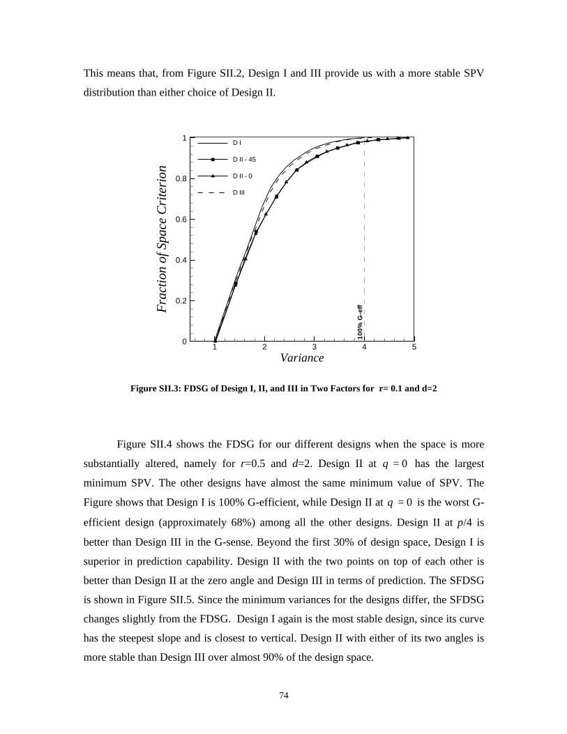
74
This means that, from Figure SII.2, Design I and III provide us with a more stable SPV
distribution than either choice of Design II.
1 2 3 4 5Variance
0
0.2
0.4
0.6
0.8
1
Frac
tion
ofSp
ace
Cri
teri
on
D I
D II - 45
D II - 0
D III
100%
G-e
ff
Figure SII.3: FDSG of Design I, II, and III in Two Factors for r= 0.1 and d=2
Figure SII.4 shows the FDSG for our different designs when the space is more
substantially altered, namely for r=0.5 and d=2. Design II at 0=θ has the largest
minimum SPV. The other designs have almost the same minimum value of SPV. The
Figure shows that Design I is 100% G-efficient, while Design II at 0=θ is the worst G-
efficient design (approximately 68%) among all the other designs. Design II at π/4 is
better than Design III in the G-sense. Beyond the first 30% of design space, Design I is
superior in prediction capability. Design II with the two points on top of each other is
better than Design II at the zero angle and Design III in terms of prediction. The SFDSG
is shown in Figure SII.5. Since the minimum variances for the designs differ, the SFDSG
changes slightly from the FDSG. Design I again is the most stable design, since its curve
has the steepest slope and is closest to vertical. Design II with either of its two angles is
more stable than Design III over almost 90% of the design space.
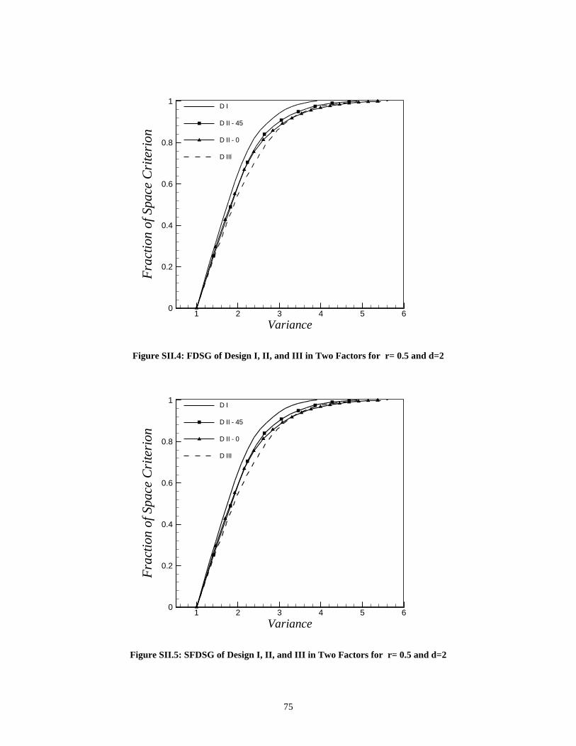
75
1 2 3 4 5 6Variance
0
0.2
0.4
0.6
0.8
1
Frac
tion
ofSp
ace
Cri
teri
on
D I
D II - 45
D II - 0
D III
Figure SII.4: FDSG of Design I, II, and III in Two Factors for r= 0.5 and d=2
1 2 3 4 5 6Variance
0
0.2
0.4
0.6
0.8
1
Frac
tion
ofSp
ace
Cri
teri
on
D I
D II - 45
D II - 0
D III
Figure SII.5: SFDSG of Design I, II, and III in Two Factors for r= 0.5 and d=2
76
SII.2 Three-Factor CaseFor the three-factor case, we compare our three designs in terms of the FDS
technique when fitting Model I. Recall that Design I shifts the (1,1,1) point to (a, a, a)
where 1<a , Design II uses three points on the sphere portion and Design III is a reduced
area full factorial. Figure SII.6 shows the FDSG of Design I in three factors for d=2 and
different values of r. The graph shows that the design is no longer G-optimal. However,
the design is highly G-efficient as the figure shows. The minimum SPV value of Design I
does not change with r. The stability of the SPV is a decreasing function of r.
Figure SII.7 depicts the FDSG of Design I, II (for angle sets 1 and 2) and III for
r=0.1 and d=2. All the designs have almost the same minimum SPV. Design III is more
G-efficient than Design II at both angles. All the designs perform almost equally in terms
of prediction within the first 25% of the design space. Design III is a real competitor to
Design I, the best design in terms of prediction. Design II at both angle sets has the least
prediction capability. Changing the angle sets does not affect the prediction capability of
Design II at r=1 and d=2 greatly. The SFDSG, in Figure SII.8 shows the superiority of
Design I in terms of the overall prediction capability. Design III is more stable than
Design II with its two angle sets.
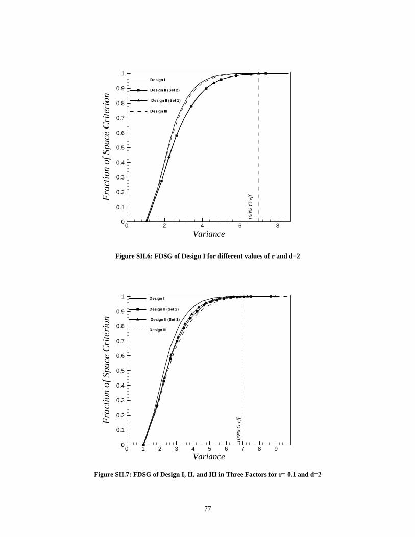
77
0 2 4 6 8Variance
0
0.1
0.2
0.3
0.4
0.5
0.6
0.7
0.8
0.9
1
Frac
tion
ofSp
ace
Cri
teri
on
Design I
Design II (Set 2)
Design II (Set 1)
Design III
100%
G-e
ffFigure SII.6: FDSG of Design I for different values of r and d=2
0 1 2 3 4 5 6 7 8 9Variance
0
0.1
0.2
0.3
0.4
0.5
0.6
0.7
0.8
0.9
1
Frac
tion
ofSp
ace
Cri
teri
on
Design I
Design II (Set 2)
Design II (Set 1)
Design III
100%
G-e
ff
Figure SII.7: FDSG of Design I, II, and III in Three Factors for r= 0.1 and d=2
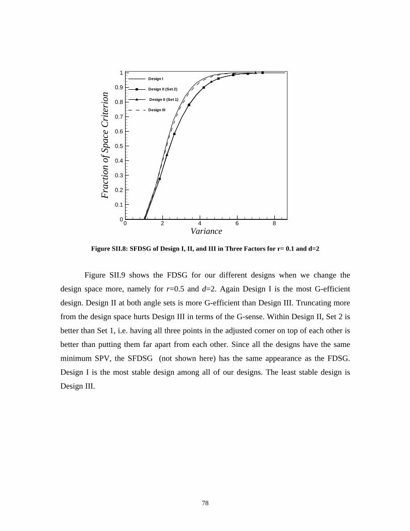
78
0 2 4 6 8Variance
0
0.1
0.2
0.3
0.4
0.5
0.6
0.7
0.8
0.9
1
Frac
tion
ofSp
ace
Cri
teri
on
Design I
Design II (Set 2)
Design II (Set 1)
Design III
Figure SII.8: SFDSG of Design I, II, and III in Three Factors for r= 0.1 and d=2
Figure SII.9 shows the FDSG for our different designs when we change the
design space more, namely for r=0.5 and d=2. Again Design I is the most G-efficient
design. Design II at both angle sets is more G-efficient than Design III. Truncating more
from the design space hurts Design III in terms of the G-sense. Within Design II, Set 2 is
better than Set 1, i.e. having all three points in the adjusted corner on top of each other is
better than putting them far apart from each other. Since all the designs have the same
minimum SPV, the SFDSG (not shown here) has the same appearance as the FDSG.
Design I is the most stable design among all of our designs. The least stable design is
Design III.
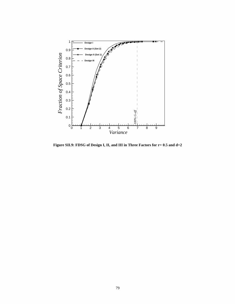
79
0 1 2 3 4 5 6 7 8 9Variance
0
0.1
0.2
0.3
0.4
0.5
0.6
0.7
0.8
0.9
1
Frac
tion
ofSp
ace
Cri
teri
on
Design I
Design II (Set 2)
Design II (Set 1)
Design III
100%
G-e
ff
Figure SII.9: FDSG of Design I, II, and III in Three Factors for r= 0.5 and d=2
80
Chapter IV Use of Standard Factorial Designs withGeneralized Linear Models
IV.1 AbstractOptimum experimental designs for generalized linear models (GLM) depend on the
values of the unknown parameters. Several solutions to the dependency of the parameters
of the optimality function were suggested in the literature. However, designs that need
good initial guesses, a complicated minimax procedure, or estimation of the unknown
parameters at each step to make the next move, are often unrealistic in practice. Rather,
one seeks designs which are simple to implement and have ‘good’ efficiencies! In this
paper, the behavior of the factorial designs, the well-known standard designs of the linear
case, is studied in the GLM case. Conditions under which these standard designs have
high G-efficiency are formulated.
IV.2 IntroductionExperimental design techniques in nonlinear model settings are needed for a
broad range of applications in the chemical, biological and clinical sciences. Often, one
faces responses such as the number of defectives out of N sampled items, the number of
defects that occur in a piece of yarn in the textile industry, or the number of organisms
that survive a pesticide or chemical treatment. For more examples, see Myers and
Montgomery (2002), Hamada and Nelder (1997), Lewis et al. (2001), or Myers,
Montgomery and Vining (2002).
Tools for design choice or design optimality in the nonlinear setting arise in
applications with non-normal responses and generalized linear models are commonly
used. But it is well known that design optimality in the nonlinear case is very difficult to
implement. The information matrix is a function of the design levels in the linear models
case, while it is also a function of the unknown parameters in the nonlinear case. In
generalized linear models (GLM), the information matrix, apart from a constant, is
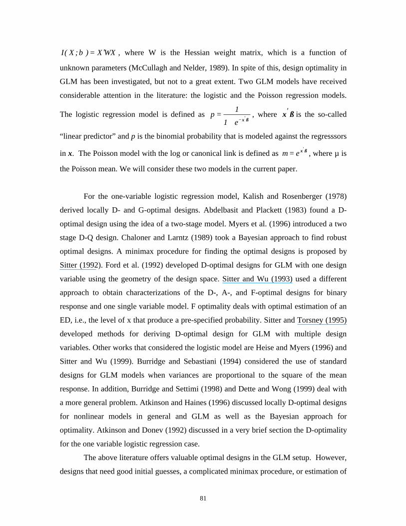
81
WXX);X(I ′=β , where W is the Hessian weight matrix, which is a function of
unknown parameters (McCullagh and Nelder, 1989). In spite of this, design optimality in
GLM has been investigated, but not to a great extent. Two GLM models have received
considerable attention in the literature: the logistic and the Poisson regression models.
The logistic regression model is defined as ßx′−+
=e1
1p , where ßx′ is the so-called
“linear predictor” and p is the binomial probability that is modeled against the regresssors
in x. The Poisson model with the log or canonical link is defined as ßx′= eµ , where µ is
the Poisson mean. We will consider these two models in the current paper.
For the one-variable logistic regression model, Kalish and Rosenberger (1978)
derived locally D- and G-optimal designs. Abdelbasit and Plackett (1983) found a D-
optimal design using the idea of a two-stage model. Myers et al. (1996) introduced a two
stage D-Q design. Chaloner and Larntz (1989) took a Bayesian approach to find robust
optimal designs. A minimax procedure for finding the optimal designs is proposed by
Sitter (1992). Ford et al. (1992) developed D-optimal designs for GLM with one design
variable using the geometry of the design space. Sitter and Wu (1993) used a different
approach to obtain characterizations of the D-, A-, and F-optimal designs for binary
response and one single variable model. F optimality deals with optimal estimation of an
ED, i.e., the level of x that produce a pre-specified probability. Sitter and Torsney (1995)
developed methods for deriving D-optimal design for GLM with multiple design
variables. Other works that considered the logistic model are Heise and Myers (1996) and
Sitter and Wu (1999). Burridge and Sebastiani (1994) considered the use of standard
designs for GLM models when variances are proportional to the square of the mean
response. In addition, Burridge and Settimi (1998) and Dette and Wong (1999) deal with
a more general problem. Atkinson and Haines (1996) discussed locally D-optimal designs
for nonlinear models in general and GLM as well as the Bayesian approach for
optimality. Atkinson and Donev (1992) discussed in a very brief section the D-optimality
for the one variable logistic regression case.
The above literature offers valuable optimal designs in the GLM setup. However,
designs that need good initial guesses, a complicated minimax procedure, or estimation of
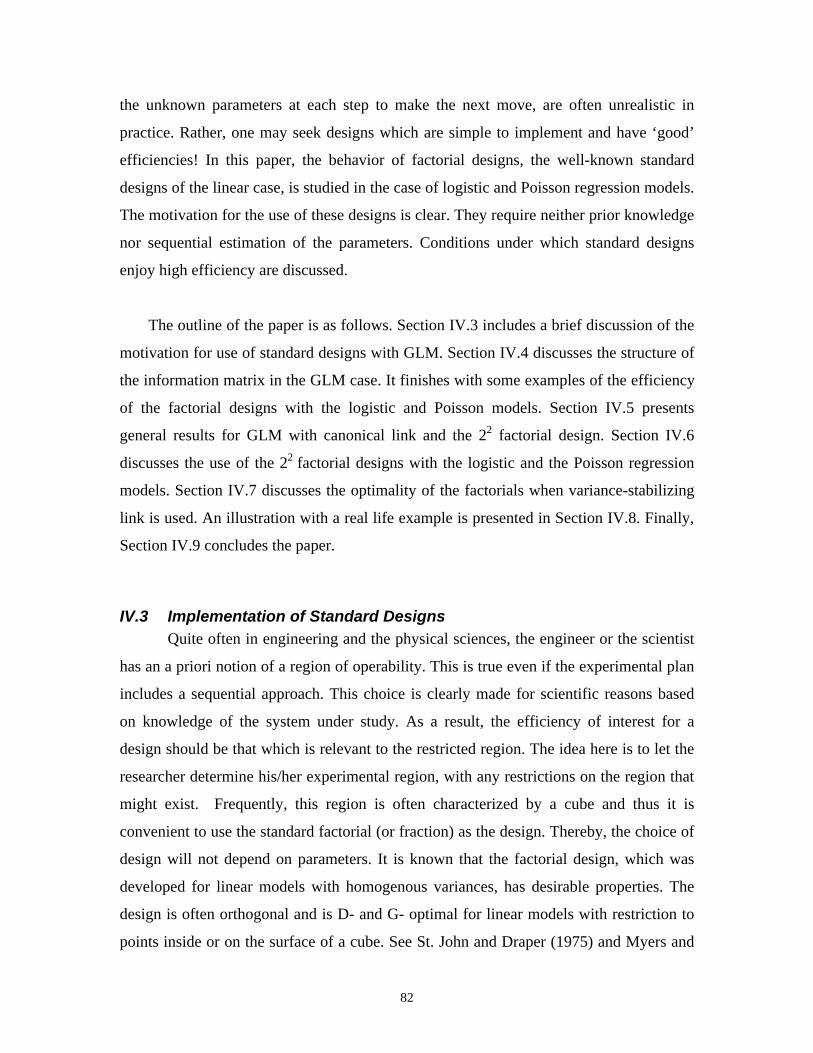
82
the unknown parameters at each step to make the next move, are often unrealistic in
practice. Rather, one may seek designs which are simple to implement and have ‘good’
efficiencies! In this paper, the behavior of factorial designs, the well-known standard
designs of the linear case, is studied in the case of logistic and Poisson regression models.
The motivation for the use of these designs is clear. They require neither prior knowledge
nor sequential estimation of the parameters. Conditions under which standard designs
enjoy high efficiency are discussed.
The outline of the paper is as follows. Section IV.3 includes a brief discussion of the
motivation for use of standard designs with GLM. Section IV.4 discusses the structure of
the information matrix in the GLM case. It finishes with some examples of the efficiency
of the factorial designs with the logistic and Poisson models. Section IV.5 presents
general results for GLM with canonical link and the 22 factorial design. Section IV.6
discusses the use of the 22 factorial designs with the logistic and the Poisson regression
models. Section IV.7 discusses the optimality of the factorials when variance-stabilizing
link is used. An illustration with a real life example is presented in Section IV.8. Finally,
Section IV.9 concludes the paper.
IV.3 Implementation of Standard DesignsQuite often in engineering and the physical sciences, the engineer or the scientist
has an a priori notion of a region of operability. This is true even if the experimental plan
includes a sequential approach. This choice is clearly made for scientific reasons based
on knowledge of the system under study. As a result, the efficiency of interest for a
design should be that which is relevant to the restricted region. The idea here is to let the
researcher determine his/her experimental region, with any restrictions on the region that
might exist. Frequently, this region is often characterized by a cube and thus it is
convenient to use the standard factorial (or fraction) as the design. Thereby, the choice of
design will not depend on parameters. It is known that the factorial design, which was
developed for linear models with homogenous variances, has desirable properties. The
design is often orthogonal and is D- and G- optimal for linear models with restriction to
points inside or on the surface of a cube. See St. John and Draper (1975) and Myers and

83
Montgomery (2002). However, the question is how efficient is the two level Factorial
design in the GLM case? The design should not be compared to any type of globally
optimal design, which will not be known and quite likely can not be implemented in the
relevant region of interest anyway.
It should be noted that despite the clear appropriateness of this class of designs for
the case of linear models, it is not clear for the GLM case. The use of generalized linear
models often involves a nonlinear model, which involves a situation where the residual
variance is a function of the mean, and thus is non-constant. While the nature of these
relationships depends on the distribution involved and the link function used, these
nonideal conditions are not the ones under which the factorial or fractional factorials
were intended. Nevertheless, we shall demonstrate that often these standard designs are
not only efficient in the GLM case but for certain situations they are D and G optimal
under the operability region restrictions assumed. We shall highlight and review some
results that are general to all GLMs and then use logistic regression and Poisson
regression as illustrations.
IV.4 Characteristics of the Information Matrix in GLMThe nature of the Fisher information matrix is an important factor in determining
the efficiency of a design for the GLM case as it is in the linear model case. The
information matrix is a quantitative measure of the quality of the information on the
parameters available in the data. It is known that the asymptotic variance covariance
matrix of the maximum likelihood estimator (MLE) is the inverse of Fisher information
matrix. The MLE of the parameter is the solution of the likelihood equations (score
function)
−=
=
∂∂
−=∂∂
∂∂
=∂
∂ ∑ 0)()(a
1)(llog)(llog in
1iii ß
yßß
θµ
φθ
θθθ
. (3.1)
where θ is the natural location parameter and φ is the dispersion parameter of the
distribution of yi, β is the vector of the unknown parameters in the model and µ is the
mean response function. For more details see McCullagh and Nelder (1989) or Myers
Montgomery and Vining (2002).

84
Using the chain rule to write ii
i
xß
ßxßxß i
)()(
?=∂
′∂′∂
∂=
∂∂ θθ
, one can write the score
function, apart from a(φ), in matrix form as 0? =−′ )(X µY , where )(diag inn ?? =× .
Apart from a(φ), the Fisher information matrix, I(X;β), is the variance of the score
function
WXXXVX))(Xvar())(llog
var();X(I ′=′=−′=∂
∂= ??? µ
θY
ßß (3.2)
where W is a diagonal matrix that contains the Hessian weights, wi, i=1,…,n. These
weights are functions of the unknown parameters. For the canonical link, the Hessian
weight matrix, W, reduces to V, a diagonal matrix that contains the variances of the
response distribution.
IV.4.1 Use of the two-level FactorialDefining XWZ 2/1= , one can write the Fisher information matrix of the GLMs
as ZZ);X(I ′=β . This has the same appearance as the information matrix for linear
models except that the Z matrix is a function of the unknown parameters. For two-level
factorials and fractional factorials with levels at 1± , the diagonal elements of I(X;β) are
sums of the Hessian weights, ∑=
n
1ii
w , while the off-diagonals are natural contrasts in the
Hessian weights, the same contrasts that produce “effects” in the linear model analysis.
For example, in the case of logistic regression these off diagonal elements are contrasts in
the binomial variances. For an illustration, consider the two-level factorial in two factors,
A and B, with only main effects
−−
−−
=
111111111111
X
=
4
3
2
1
w0000w0000w0000w
W
The information matrix is then
=
∑∑
∑
i
i
i
wContrABContrBContrABwContrAContrBContrAw
)(I β

85
where ContrA is a contrast of A on the Hessian weights, ContrAB is a contrast of the
interaction effect of the two factors A and B on the Hessian weights, which appears in the
information matrix despite the fact that there is no interaction in the model. For more
details, see Myers et al. (2002). The Fisher information matrix will be well conditioned if
these off-diagonals are near zero. Usually, the sum of the Hessian weights will dominate
the off diagonal elements. The Hessian weights for the case of canonical link are merely
the variances of the distribution; and the contrasts in the distribution variance are
certainly dominated by the sum, resulting in a well-conditioned information matrix.
Hence, in this case, good efficiency of the two-level factorial design is expected.
IV.4.2 ExamplesIn this section some hypothetical examples are used to show the G-efficiency of
the 22 factorial design for the case of the logistic and Poisson regression models. The
measure of design efficiency proposed by Myers et al. (2002), which compares the
asymptotic variances of individual coefficients with that obtained if the same Hessian
weights were observed with an orthogonal design, is calculated. This kind of efficiency
gives a sense of the ill conditioning level of the information matrix. In the present article,
we will refer to this kind of efficiency as efficiency of parameter estimates. These
values are very much like variance inflation factors in regression analysis. The
asymptotic variances of the coefficients are also computed and the contour plots of the
scaled prediction variance are shown.
Example 1: Consider the 22 factorial design with a first order model in the linear
predictor in the case of logistic regression. Parameter values are chosen so that the
binomial parameter in the design region is 6.0p4.0 ≤≤ . The G-efficiency of the
factorial design is 99.4%. This reflects the high level of conditioning of the information
matrix in this case. The asymptotic variance covariance matrix is
−−=−
05115.000092.0000092.005115.000005113.0
);X(I 1 β
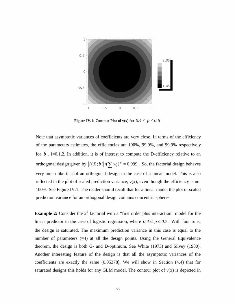
86
Figure IV.1: Contour Plot of v(x) for 6.0p4.0 ≤≤
Note that asymptotic variances of coefficients are very close. In terms of the efficiency
of the parameters estimates, the efficiencies are 100%, 99.9%, and 99.9% respectively
for iβ̂ , i=0,1,2. In addition, it is of interest to compute the D-efficiency relative to an
orthogonal design given by 999.0)/();( =∑ piwXI β . So, the factorial design behaves
very much like that of an orthogonal design in the case of a linear model. This is also
reflected in the plot of scaled prediction variance, v(x), even though the efficiency is not
100%. See Figure IV.1. The reader should recall that for a linear model the plot of scaled
prediction variance for an orthogonal design contains concentric spheres.
Example 2: Consider the 22 factorial with a “first order plus interaction” model for the
linear predictor in the case of logistic regression, where 7.0p4.0 ≤≤ . With four runs,
the design is saturated. The maximum prediction variance in this case is equal to the
number of parameters (=4) at all the design points. Using the General Equivalence
theorem, the design is both G- and D-optimum. See White (1973) and Silvey (1980).
Another interesting feature of the design is that all the asymptotic variances of the
coefficients are exactly the same (0.05378). We will show in Section (4.4) that for
saturated designs this holds for any GLM model. The contour plot of v(x) is depicted in
-1 -0.5 0 0.5 1-1
-0.5
0
0.5
1
1.45
2.95
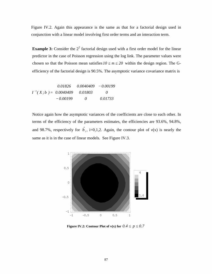
87
Figure IV.2. Again this appearance is the same as that for a factorial design used in
conjunction with a linear model involving first order terms and an interaction term.
Example 3: Consider the 22 factorial design used with a first order model for the linear
predictor in the case of Poisson regression using the log link. The parameter values were
chosen so that the Poisson mean satisfies 2010 ≤≤ µ within the design region. The G-
efficiency of the factorial design is 90.5%. The asymptotic variance covariance matrix is
−
−=−
01733.0000199.0001803.00040409.000199.00040409.001826.0
);X(I 1 β
Notice again how the asymptotic variances of the coefficients are close to each other. In
terms of the efficiency of the parameters estimates, the efficiencies are 93.6%, 94.8%,
and 98.7%, respectively for iβ̂ , i=0,1,2. Again, the contour plot of v(x) is nearly the
same as it is in the case of linear models. See Figure IV.3.
Figure IV.2: Contour Plot of v(x) for 7.0p4.0 ≤≤
-1 -0.5 0 0.5 1-1
-0.5
0
0.5
1
1.6
4
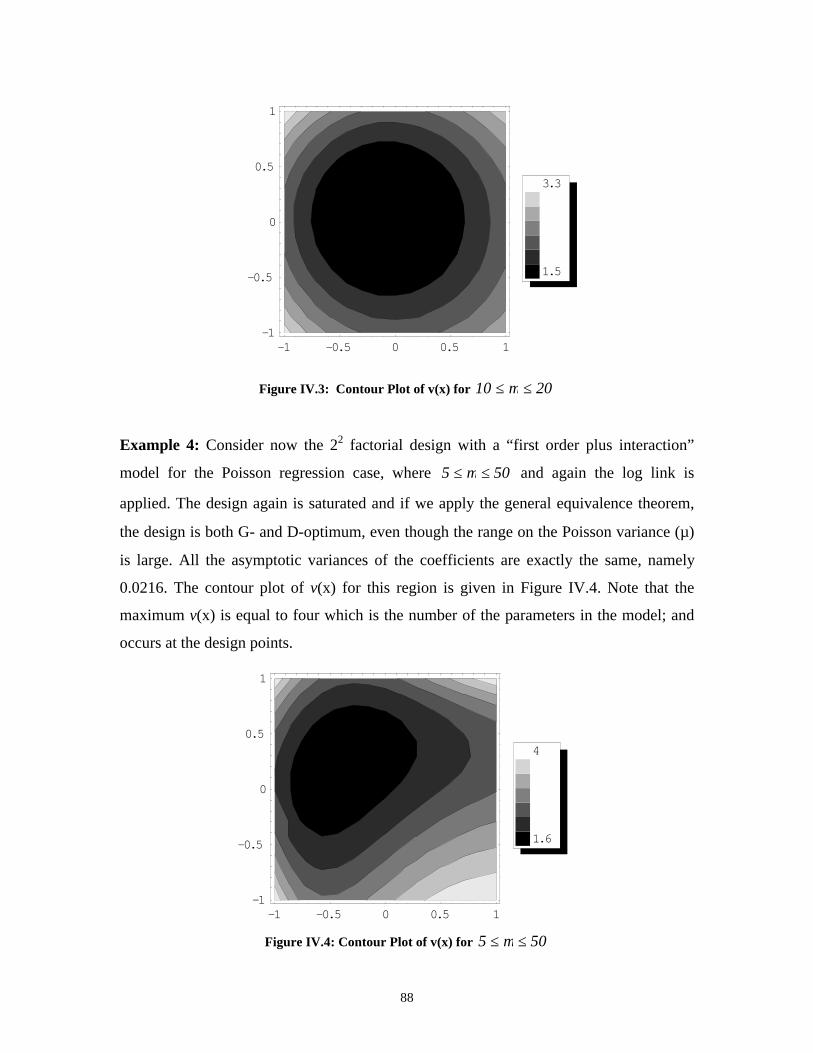
88
Figure IV.3: Contour Plot of v(x) for 2010 ≤≤ µ
Example 4: Consider now the 22 factorial design with a “first order plus interaction”
model for the Poisson regression case, where 505 ≤≤ µ and again the log link is
applied. The design again is saturated and if we apply the general equivalence theorem,
the design is both G- and D-optimum, even though the range on the Poisson variance (µ)
is large. All the asymptotic variances of the coefficients are exactly the same, namely
0.0216. The contour plot of v(x) for this region is given in Figure IV.4. Note that the
maximum v(x) is equal to four which is the number of the parameters in the model; and
occurs at the design points.
Figure IV.4: Contour Plot of v(x) for 505 ≤≤ µ
-1 -0.5 0 0.5 1-1
-0.5
0
0.5
1
1.6
4
-1 -0.5 0 0.5 1-1
-0.5
0
0.5
1
1.5
3.3

89
The foregoing examples illustrate that the 22 factorial can be very efficient and even
optimal in some cases for Poisson and logistic regression. Obviously, the efficiency
depends on the values of the mean (and thus the variance) of the distribution. In what
follows we shall provide some more formal details.
IV.5 General Results for GLM with Canonical Link and Standard 22
Factorial DesignOne can show that in the GLM case, the factorial design is quite efficient both in
the D and G sense if the model contains first order and interaction terms except in certain
rather unusual cases. Actually, we considered only the G-efficiency since the D
efficiency is difficult to calculate. It is well known that the G-efficiency is a lower bound
for the D-efficiency, see Atwood (1969). One can show also that under some conditions
the factorial design achieves optimality.
Let us define v4 as the maximum variance of the distribution among all the design
locations. Similarly, let v1 be the minimum. We will assume without loss of generality
that these variances are achieved at (1,1) and (-1,-1). Assume further that v2 and v3 are the
variances at the other two design points. In what follows we characterize how the
distribution variance at the design points influences the scaled prediction variance.
Clearly, if the distribution variance throughout the design region has a very small
dispersion, one would expect the factorial design to have high efficiency. The scaled
prediction variance, employing the canonical link, can be written as1
00 )VXX(v)n4()(v −′=x , where v0 is the distribution variance at the point 0x in question.
IV.5.1 Properties of the Scaled Prediction Variance for the 22 Factorial DesignLet us first assume that the linear predictor contains a first order model. In Appendix
A, we present an equivalent expression for )(v 0x which is written in terms of ratios of
the distribution variances, v1, v2, v3, v4 and v0. The result is found in Appendix A equation
(A.1). Assume further that 40,321
vvv,vv ≤≤ , then the following important results
become clear.

90
1) the scaled prediction variance is a function of the ratio 1
4
v
v=δ
2) the G-efficiency of the design is a decreasing function of δ .
Now, let us suppose that v0 is larger than any one of the variances at the design
points. For example in the case of logistic regression, the ED50 may be inside the design
region. Then we have max04321
vvvvvv ≤≤≤≤≤ , where vmax is the largest variance in
the design region. It turns out that )(v 0x is a function of 4max4 v/v=δ and δ. Hence, the
G-efficiency is also a function of both of these ratios. In fact it is a decreasing function of
both ratios. Our empirical studies show that the impact of δ is much greater than δ4.
Assume now that the linear predictor contains first order plus interaction terms. As in
the case of the no interaction model we develop the expression for the scaled prediction
variance in terms of ratios of the distribution variances, v1, v2, v3, v4 and v0 in Appendix
A. In this case, the expression is simpler and is given by
]}ffvv
fvv
f[v1
{4
nv )x(v 43
3
42
2
41
4
00 +++= δ
where 22
211 )1x()1x(f −−= , 2
12
22 )1x()1x(f −+= , 22
213 )1x()1x(f −+= and
21
224 )1x()1x(f ++= .
Using the same argument as in the no interaction model, the G-efficiency of the 22
design is a decreasing function of the ratio δ. In this case, the value of v4 and its
relationship to vmax does not play a role (see Appendix A).
In the Section V, we will use this important result for the logistic and Poisson case to
ascertain conditions in which standard factorials are highly efficient. However, we first
reveal some highly desirable properties of the 22 factorial design in the case of the
interaction model for GLMs in which the canonical link is used. We noticed these
conditions in examples given in Section 3.2. The properties relate to the coefficient
variances and the nature of the maximum prediction variance.
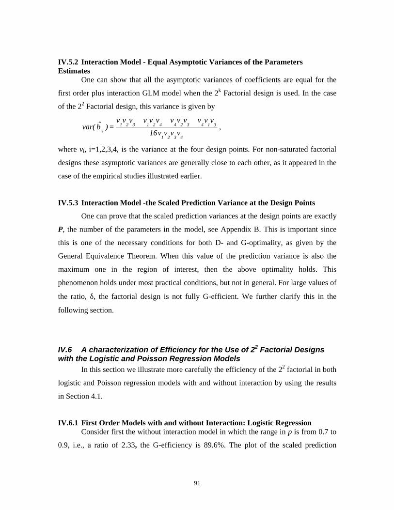
91
IV.5.2 Interaction Model - Equal Asymptotic Variances of the ParametersEstimates
One can show that all the asymptotic variances of coefficients are equal for the
first order plus interaction GLM model when the 2k Factorial design is used. In the case
of the 22 Factorial design, this variance is given by
4321
314324421321i vvvv16
vvvvvvvvvvvv)ˆvar(
+++=β ,
where vi, i=1,2,3,4, is the variance at the four design points. For non-saturated factorial
designs these asymptotic variances are generally close to each other, as it appeared in the
case of the empirical studies illustrated earlier.
IV.5.3 Interaction Model -the Scaled Prediction Variance at the Design Points
One can prove that the scaled prediction variances at the design points are exactly
P, the number of the parameters in the model, see Appendix B. This is important since
this is one of the necessary conditions for both D- and G-optimality, as given by the
General Equivalence Theorem. When this value of the prediction variance is also the
maximum one in the region of interest, then the above optimality holds. This
phenomenon holds under most practical conditions, but not in general. For large values of
the ratio, δ, the factorial design is not fully G-efficient. We further clarify this in the
following section.
IV.6 A characterization of Efficiency for the Use of 22 Factorial Designswith the Logistic and Poisson Regression Models
In this section we illustrate more carefully the efficiency of the 22 factorial in both
logistic and Poisson regression models with and without interaction by using the results
in Section 4.1.
IV.6.1 First Order Models with and without Interaction: Logistic RegressionConsider first the without interaction model in which the range in p is from 0.7 to
0.9, i.e., a ratio of 2.33, the G-efficiency is 89.6%. The plot of the scaled prediction
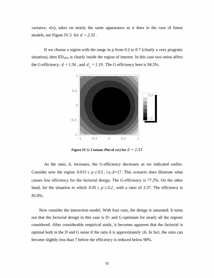
92
variance, v(x), takes on nearly the same appearance as it does in the case of linear
models, see Figure IV.5 for 33.2=δ .
If we choose a region with the range in p from 0.2 to 0.7 (clearly a very progratic
situation), then ED50% is clearly inside the region of interest. In this case two ratios affect
the G-efficiency: 56.1=δ , and 19.14
=δ . The G-efficiency here is 94.5%.
Figure IV.5: Contour Plot of v(x) for 33.2=δ
As the ratio, δ, increases, the G-efficiency decreases as we indicated earlier.
Consider now the region 5.0p015.0 ≤≤ , i.e.,δ=17. This scenario does illustrate what
causes low efficiency for the factorial design. The G-efficiency is 77.2%. On the other
hand, for the situation in which 2.0p05.0 ≤≤ , with a ratio of 3.37. The efficiency is
85.8%.
Now consider the interaction model. With four runs, the design is saturated. It turns
out that the factorial design in this case is D- and G-optimum for nearly all the regions
considered. After considerable empirical study, it becomes apparent that the factorial is
optimal both in the D and G sense if the ratio δ is approximately ≤6. In fact, the ratio can
become slightly less than 7 before the efficiency is reduced below 90%.
-1 -0.5 0 0.5 1-1
-0.5
0
0.5
1
1.5
3.3
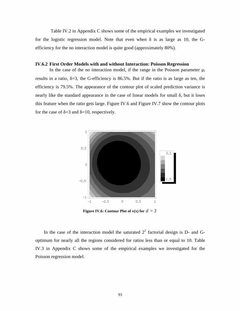
93
Table IV.2 in Appendix C shows some of the empirical examples we investigated
for the logistic regression model. Note that even when δ is as large as 10, the G-
efficiency for the no interaction model is quite good (approximately 80%).
IV.6.2 First Order Models with and without Interaction: Poisson RegressionIn the case of the no interaction model, if the range in the Poisson parameter µi
results in a ratio, δ=3, the G-efficiency is 86.5%. But if the ratio is as large as ten, the
efficiency is 79.5%. The appearance of the contour plot of scaled prediction variance is
nearly like the standard appearance in the case of linear models for small δ, but it loses
this feature when the ratio gets large. Figure IV.6 and Figure IV.7 show the contour plots
for the case of δ=3 and δ=10, respectively.
Figure IV.6: Contour Plot of v(x) for 3=δ
In the case of the interaction model the saturated 22 factorial design is D- and G-
optimum for nearly all the regions considered for ratios less than or equal to 10. Table
IV.3 in Appendix C shows some of the empirical examples we investigated for the
Poisson regression model.
-1 -0.5 0 0.5 1-1
-0.5
0
0.5
1
1.5
3.3
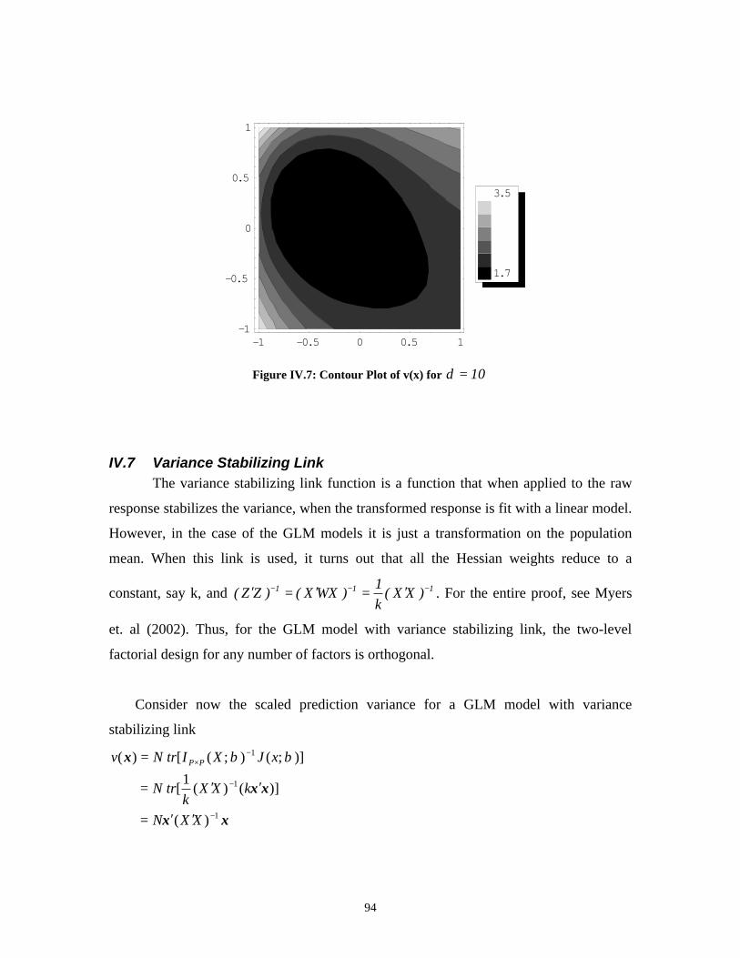
94
Figure IV.7: Contour Plot of v(x) for 10=δ
IV.7 Variance Stabilizing LinkThe variance stabilizing link function is a function that when applied to the raw
response stabilizes the variance, when the transformed response is fit with a linear model.
However, in the case of the GLM models it is just a transformation on the population
mean. When this link is used, it turns out that all the Hessian weights reduce to a
constant, say k, and 111 )XX(k1
)WXX()ZZ( −−− ′=′=′ . For the entire proof, see Myers
et. al (2002). Thus, for the GLM model with variance stabilizing link, the two-level
factorial design for any number of factors is orthogonal.
Consider now the scaled prediction variance for a GLM model with variance
stabilizing link
xx
xx
x
1
1
1
)(
)]()(1
[
)];();([ )(
−
−
−×
′′=
′′=
=
XXN
kXXk
trN
xJXItrNv PP ββ
-1 -0.5 0 0.5 1-1
-0.5
0
0.5
1
1.7
3.5
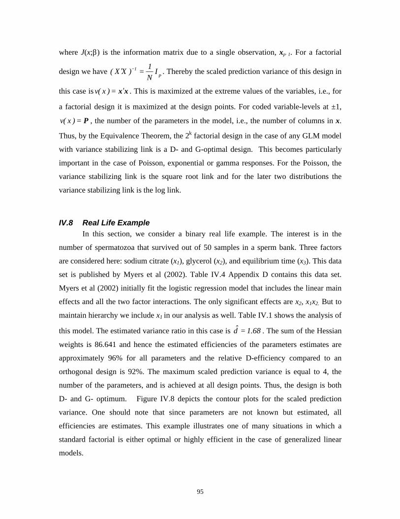
95
where J(x;β) is the information matrix due to a single observation, xp×1. For a factorial
design we have P
1 IN1
)XX( =′ − . Thereby the scaled prediction variance of this design in
this case is xx′=)x(v . This is maximized at the extreme values of the variables, i.e., for
a factorial design it is maximized at the design points. For coded variable-levels at ±1,
P=)x(v , the number of the parameters in the model, i.e., the number of columns in x.
Thus, by the Equivalence Theorem, the 2k factorial design in the case of any GLM model
with variance stabilizing link is a D- and G-optimal design. This becomes particularly
important in the case of Poisson, exponential or gamma responses. For the Poisson, the
variance stabilizing link is the square root link and for the later two distributions the
variance stabilizing link is the log link.
IV.8 Real Life ExampleIn this section, we consider a binary real life example. The interest is in the
number of spermatozoa that survived out of 50 samples in a sperm bank. Three factors
are considered here: sodium citrate (x1), glycerol (x2), and equilibrium time (x3). This data
set is published by Myers et al (2002). Table IV.4 Appendix D contains this data set.
Myers et al (2002) initially fit the logistic regression model that includes the linear main
effects and all the two factor interactions. The only significant effects are x2, x1x2. But to
maintain hierarchy we include x1 in our analysis as well. Table IV.1 shows the analysis of
this model. The estimated variance ratio in this case is 68.1ˆ =δ . The sum of the Hessian
weights is 86.641 and hence the estimated efficiencies of the parameters estimates are
approximately 96% for all parameters and the relative D-efficiency compared to an
orthogonal design is 92%. The maximum scaled prediction variance is equal to 4, the
number of the parameters, and is achieved at all design points. Thus, the design is both
D- and G- optimum. Figure IV.8 depicts the contour plots for the scaled prediction
variance. One should note that since parameters are not known but estimated, all
efficiencies are estimates. This example illustrates one of many situations in which a
standard factorial is either optimal or highly efficient in the case of generalized linear
models.
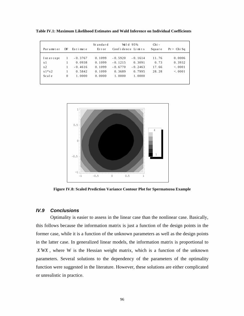
96
Table IV.1: Maximum Likelihood Estimates and Wald Inference on Individual Coefficients
Figure IV.8: Scaled Prediction Variance Contour Plot for Spermatozoa Example
IV.9 ConclusionsOptimality is easier to assess in the linear case than the nonlinear case. Basically,
this follows because the information matrix is just a function of the design points in the
former case, while it is a function of the unknown parameters as well as the design points
in the latter case. In generalized linear models, the information matrix is proportional to
WXX ′ , where W is the Hessian weight matrix, which is a function of the unknown
parameters. Several solutions to the dependency of the parameters of the optimality
function were suggested in the literature. However, these solutions are either complicated
or unrealistic in practice.
Standard Wald 95% Chi-Parameter DF Estimate Error Confidence Limits Square Pr> ChiSq
Intercept 1 -0.3767 0.1099 -0.5920 -0.1614 11.76 0.0006x1 1 0.0938 0.1099 -0.1215 0.3091 0.73 0.3932x2 1 -0.4616 0.1099 -0.6770 -0.2463 17.66 <.0001x1*x2 1 0.5842 0.1099 0.3689 0.7995 28.28 <.0001Scale 0 1.0000 0.0000 1.0000 1.0000
-1 -0.5 0 0.5 1-1
-0.5
0
0.5
1
1
4
97
In this paper, the behavior of factorial designs, the well-known standard designs
of the linear case, has been studied. Although the generalized linear models often results
in non-ideal conditions under which the standard designs were never intended to be used,
these designs are not only efficient but for certain situations they are D and G optimal.
We formulated conditions under which these standard designs have high G-efficiency.
The use of these designs in the GLM case is illustrated with examples from the logistic
and Poisson regression models.
Other desirable properties of the factorial designs are discussed in this paper. In the
case of the interaction model for GLMs in which the canonical link is used, the 2k
factorial design ensures equal asymptotic variances of the estimated coefficients and that
the maximum prediction variance at the design point is equal to the number of the
parameters. Also, by the Equivalence Theorem, the 2k factorial design in the case of any
GLM model with variance stabilizing link is a D- and G-optimal design. This becomes
particularly important in the case of Poisson, exponential or gamma responses.
IV.10 ReferencesAbdelbasit, K. M. and Plackett, R. L. (1983), “Experimental Design for Binary Data”,
Journal of the American Statistical Association, 78, 90-98.
Atkinson, A. C. and Donev, A. N. (1992), Optimum Experimental Designs, Oxford
University Press, Oxford.
Atkinson, A. C. and Haines, L. M. (1996), “Designs for Nonlinear and Generalized
Linear Models”, In: S. Ghosh and C.R Rao, eds., Handbook of Statistics, 13,
Elsevier Science B.V, 437-475.
Burridge, J. and Sebastiani, P. (1992), “D-optimal Designs for Generalised Linear
Models”, Journal Ital. Stat. Soc., 2, 182-202.
Burridge, J. and Sebastiani, P. (1994), “D-optimal Designs for Generalised Linear
Models with Variance Proportional to the Square of the Mean”, Biometrika, 81,
295-304.
98
Chaloner K. and Larntz, K. (1989), “Optimal Bayesian Design Applied to Logistic
Regression Experiments”, Journal of Statistical Planning and Inference, 21, 191-
208.
Chaloner, K. and Verdinelli, I. (1995), “Bayesian Experimental Design: A Review”,
University of Minnesota Technical Report.
Chaudhuri, P. and Mykland, P. A. (1993), “Nonlinear Experiments: Optimal Design and
Inference Based on Likelihood”, Journal of the American Statistical Association,
88, 583-546.
Chernoff, H. (1953), “Locally Optimal Designs for Estimating Parameters”, Annals of
Mathematical Statistics, 24, 586-602.
Chernoff, H. (1979), Sequential Analysis and Optimal Designs, SIAM, Philadelphia, PA.
Dette, H. and Wong, W.K. (1999), “Optimal Designs When the Variance is a Function of
the Mean”, Biometrics, 55, 925-929
Ford, I., Torsney, B., and Wu, C.F.J (1992), “The Use of a Canonical Form in the
Construction of Locally Optimal Designs for Nonlinear Problems”, Journal of the
Royal Statistical Society, Ser B, 54, 569-583.
Hamada, M. and Nelder, J.A. (1997), ``Generalized Linear Models for Quality-
Improvement Experiments'', Journal of Quality Technology, 29, 292-304.
Heise, M.A. and Myers, R. H. (1996), “Optimal Designs for Bivariate Logistic
Regression”, Biometrics, 52, 613-624.
Kalish, L. A. and Rosenberger, J. L. (1978), “Optimal Designs for the Estimation of the
Logistic Function”, Technical Report 33, Pennsylvania State University.
Kiefer, J. and Wolfowitz, J. (1960), “The Equivalence of Two Extremum Problems”,
Cand. J. Math,12, 363-366.
Lewis, S., Montgomery, D. and Myers R. (2001), “Examples of Designed Experiments
with Nonnormal Responses”, Journal of Quality Technology, 33, 265-278.
Martin, B., Parker, D. and Zenick, L. (1987), “Minimize Slugging by Optimizing
Controllable Factors on Topaz Windshield Modeling”, Fifth Symposium on
Taguchi Methods. American Supplier Institute, Inc., Dearborn, MI, 519-526.
McCullagh, P. and Nelder, J.A. (1989), Generalized Linear Models, 2nd edition, New
York, Chapman and Hall.

99
Minkin, S. (1987), “Optimal Designs for Binary Data”, Journal of the American
Statistical Association, 82,1098-1103.
Myers, R.H. and Montgomery, D. C. (1997), “A Tutorial on Generalized Linear Models”,
Journal of Quality Technology, 29, 274-291.
Myers, R.H. and Montgomery, D. C. (2002), Response Surface Methodology: Process
and Product Optimization Using Designed Experiments, 2nd edition, Wiley.
Myers, R.H., Montgomery, D. C., and Vining, G.G. (2002), Generalized Linear Models
with Applications in Engineering and the Sciences, Wiley Series in Probability and
Statistics.
Myers, W. R., Myers, R.H., and Carter, W.H. Jr. (1994), “Some Alphabetic Optimal
Designs for the Logistic Regression Model”, Journal of Statistical Planning and
Inference, 42, 57-77.
Myers, W. R., Myers, R.H., Carter, W.H. Jr., and White, K. L. (1996), “Two Stage
Designs for the Logistic Regression Model in a Single Agent Bioassay”, Journal of
Biopharmaceutical Statistics, 6(4).
Sebastiani, P. and Settimi, R. (1998), “First-order Optimal Designs for Non-linear
Models”, Journal of Statistical Planning and Inference, 74, 177-192.
Sitter R. R. (1992), “Robust Designs for Binary Data”, Biometrics, 48, 1145-1155.
Sitter R. R. and Torsney, B. (1995), “D-Optimal Designs for Generalized Linear
Models”, In: C.P. Kitsos and W.G. Müller, eds., MODA 4 - Advances in Modern
Data Analysis: Proceedings (the 4th international wokshop in Spetses, Greece, June
5-9, 1995). Heidelberg, Germany: Physica-Verlag, 87-102.
Sitter, R. R. and Wu, C. F. J. (1993), “On the Accuracy of Fieller Intervals for Binary
Response Data”, Journal of the American Statistical Association, 88, 1021-1025.
Sitter, R. R. and Wu, C. F. J. (1999), “Two-Stage Design of Quantal Response Studies”,
Biometrics, 55,396-402
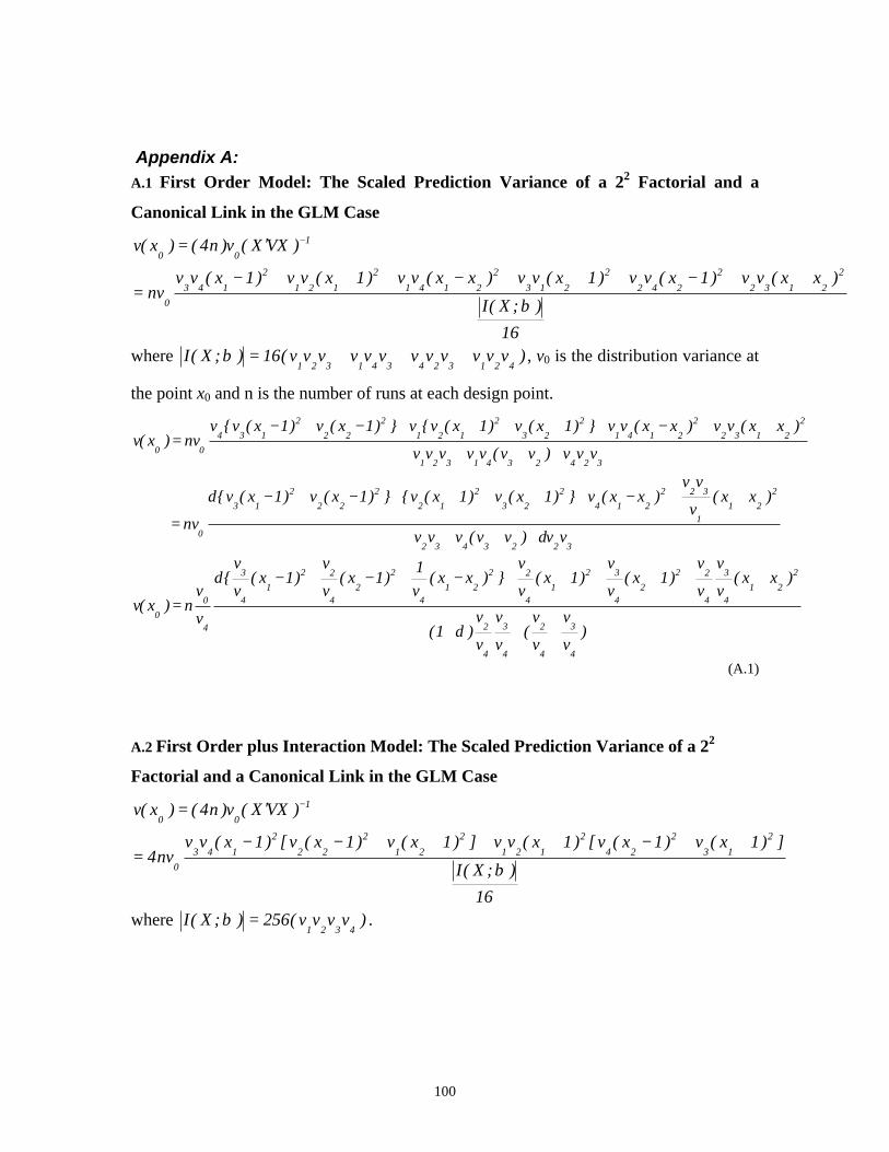
100
Appendix A:A.1 First Order Model: The Scaled Prediction Variance of a 22 Factorial and a
Canonical Link in the GLM Case
16
);X(I
)xx(vv)1x(vv)1x(vv)xx(vv)1x(vv)1x(vvnv
)VXX(v)n4()x(v2
2132
2
242
2
213
2
2141
2
121
2
1430
1
00
β
++−+++−+++−=
′= −
where )vvvvvvvvvvvv(16);X(I421324341321
+++=β , v0 is the distribution variance at
the point x0 and n is the number of runs at each design point.
3223432
2
211
322
214
2
23
2
12
2
22
2
13
0
3242341321
2
2132
2
2141
2
23
2
121
2
22
2
134
00
vv)vv(vvv
)xx(v
vv)xx(v})1x(v)1x(v{})1x(v)1x(v{
nv
vvv)vv(vvvvv
)xx(vv)xx(vv})1x(v)1x(v{v})1x(v)1x(v{vnv)x(v
δ
δ
+++
++−+++++−+−
=
+++
++−+++++−+−=
)v
v
v
v(
v
v
v
v)1(
)xx(v
v
v
v)1x(
v
v)1x(
v
v})xx(
v1
)1x(v
v)1x(
v
v{
v
vn)x(v
4
3
4
2
4
3
4
2
2
214
3
4
22
24
32
14
22
214
2
24
22
14
3
4
0
0
+++
++++++−+−+−
=
δ
δ
(A.1)
A.2 First Order plus Interaction Model: The Scaled Prediction Variance of a 22
Factorial and a Canonical Link in the GLM Case
16
);X(I
])1x(v)1x(v[)1x(vv])1x(v)1x(v[)1x(vvnv4
)VXX(v)n4()x(v2
13
2
24
2
121
2
21
2
22
2
1430
1
00
β
++−++++−−=
′= −
where )vvvv(256);X(I4321
=β .

101
]}ffv
vf
v
vf[
v1
{4
nv
}v
)1x()1x(
v
)1x()1x(
v
)1x()1x(
v
)1x()1x({
4
nv)x(v
433
42
2
41
4
0
4
2
2
2
1
3
2
2
2
1
2
2
1
2
2
1
2
2
2
100
+++=
+++
−++
−++
−−=
δ
(A.2)
where 22
211 )1x()1x(f −−= , 2
12
22 )1x()1x(f −+= , 22
213 )1x()1x(f −+= and
21
224 )1x()1x(f ++=
1) Assume 40,321
vvv,vv ≤≤
The prediction variance is an increasing function in the ratio δ. Therefore, the G-
efficiency is a decreasing function in this ratio. Note that
1v
v1
4
0 ≤≤δ
, δ≤≤2
4
v
v1 and δ≤≤
3
4
v
v1 .
2) Assume max04321
vvvvvv ≤≤≤≤≤
The prediction variance is an increasing function of the ratio δ; hence as before the G-
efficiency is a decreasing function in this ratio. Note that
4
max4
4
0
v
v
v
v1 =≤≤ δ , δ≤≤
2
4
v
v1 and δ≤≤
3
4
v
v1 .
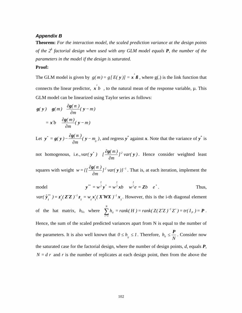
102
Appendix BTheorem: For the interaction model, the scaled prediction variance at the design points
of the 2k factorial design when used with any GLM model equals P, the number of the
parameters in the model if the design is saturated.
Proof:
The GLM model is given by ßxy ′== )](E[g)(g µ , where g(.) is the link function that
connects the linear predictor, β′x , to the natural mean of the response variable, µ. This
GLM model can be linearized using Taylor series as follows:
)()(
)()(
)()(
µµµ
β
µµµ
µ
−∂
∂+′=
−∂
∂+≅
yg
x
yg
gyg
Let )()(
)(0
* µµµ
−∂
∂−= y
gygy , and regress y* against x. Note that the variance of y* is
not homogenous, i.e., )var(])(
[)var( 2* yg
yµµ
∂∂
≅ . Hence consider weighted least
squares with weight 12 )}var(])(
{[w −
∂∂
= yg
µµ
. That is, at each iteration, implement the
model *21
21
*21
** www εβεβ +=+== Zxyy . Thus,
iiiiiixWXXxzZZzy 11** )(w)()ˆvar( −− ′′=′′= . However, this is the i-th diagonal element
of the hat matrix, hii, where P==′′== −
=∑ )I(tr)Z)ZZ(Z(rank)H(rankh P
1N
1iii .
Hence, the sum of the scaled predicted variances apart from N is equal to the number of
the parameters. It is also well known that 1h0ii
≤≤ . Therefore, N
hiiP
≤ . Consider now
the saturated case for the factorial design, where the number of design points, d, equals P,
r dN = and r is the number of replicates at each design point, then from the above the

103
ith diagonal element r1
hii = , thus the scaled prediction variance at the ith design point is
P==rN
)x(v .
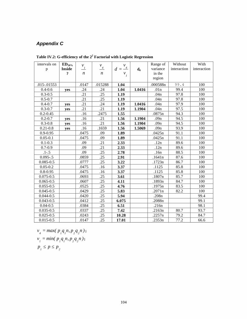
104
Appendix C
Table IV.2: G-efficiency of the 22 Factorial with Logistic Regression
intervals onp
ED50%
Inside? n
v1
n
v4
1
4
v
v=δ δ4
Range ofvariance
in theregion
Withoutinteraction
Withinteraction
.015-.01553 .0147 .015288 1.04 .000588n 99.4 1000.4-0.6 yes .24 .24 1.04 1.0416 .01n 99.4 1000.3-0.5 .21 .25 1.19 .04n 97.8 1000.5-0.7 .21 .25 1.19 .04n 97.8 1000.4-0.7 yes .21 .24 1.19 1.0416 .04n 97.9 1000.3-0.7 yes .21 .21 1.19 1.1904 .04n 97.5 100
0.2-0.45 .16 .2475 1.55 .0875n 94.3 1000.2-0.7 yes .16 .21 1.56 1.1904 .09n 94.5 1000.3-0.8 yes .16 .21 1.56 1.1904 .09n 94.5 100
0.21-0.8 yes .16 .1659 1.56 1.5069 .09n 93.9 1000.9-0.95 .0475 .09 1.89 .0425n 91.1 1000.05-0.1 .0475 .09 1.89 .0425n 91.1 1000.1-0.3 .09 .21 2.33 .12n 89.6 1000.7-0.9 .09 .21 2.33 .12n 89.6 100
.1-.5 .09 .25 2.78 .16n 88.5 1000.095-.5 .0859 .25 2.91 .1641n 87.6 1000.085-0.5 .0777 .25 3.22 .1723n 86.7 1000.05-0.2 .0475 .16 3.37 .1125 85.8 1000.8-0.95 .0475 .16 3.37 .1125 85.8 1000.075-0.5 .0693 .25 3.61 .1807n 85.7 1000.065-0.5 .0607 .25 4.11 .1893n 84.7 1000.055-0.5 .0525 .25 4.76 .1975n 83.5 1000.045-0.5 .0429 .25 5.83 .2071n 82.2 1000.044-0.5 .0420 .25 5.94 .208n 99.40.043-0.5 .0412 .25 6.075 .2088n 99.10.04-0.5 .0384 .25 6.51 .216n 98.10.035-0.5 .0337 .25 7.42 .2163n 80.7 93.70.025-0.5 .0243 .25 10.28 .2257n 79.2 84.70.015-0.5 .0147 .25 17.01 .2353n 77.2 66.6
)nqp,nqpmax(v22114
= ;
)nqp,nqpmin(v22111
= ;
21ppp ≤≤
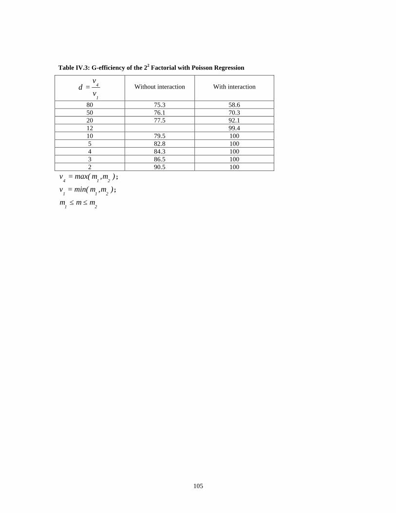
105
Table IV.3: G-efficiency of the 22 Factorial with Poisson Regression
1
4
v
v=δ Without interaction With interaction
80 75.3 58.650 76.1 70.320 77.5 92.112 99.410 79.5 1005 82.8 1004 84.3 1003 86.5 1002 90.5 100
),max(v214
µµ= ;
),min(v211
µµ= ;
21µµµ ≤≤
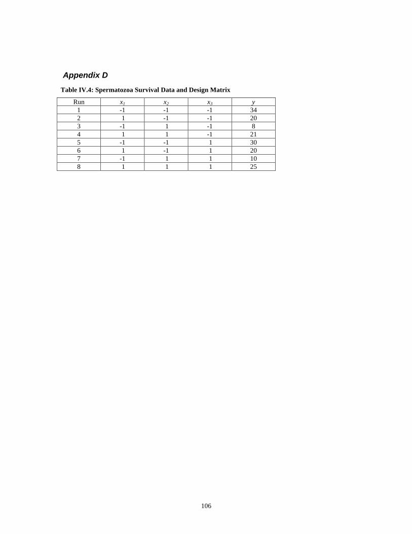
106
Appendix D
Table IV.4: Spermatozoa Survival Data and Design Matrix
Run x1 x2 x3 y1 -1 -1 -1 342 1 -1 -1 203 -1 1 -1 84 1 1 -1 215 -1 -1 1 306 1 -1 1 207 -1 1 1 108 1 1 1 25
107
Chapter V Summary and Future Work
The research contains three main contributions. First, we introduce a new
graphical technique, the Fraction of Design Space (FDS) technique, which shows how the
performance of the prediction variance changes from the center of the design out to the
perimeter. Some second order response surface designs are studied in terms of this new
measure. Secondly, for the two- and three-factor case with one corner of the cuboidal
design space excluded, three sensible alternative designs are studied and compared.
These designs involve reducing the factor levels to make a smaller but standard factorial
design fit or modifying the levels of the variables at the excluded corner to locate it in the
feasible design region. Properties of these designs and relative tradeoffs are discussed.
The alternative designs are studied in terms of the new criteria FDS. Thirdly, we study
the performance of standard designs for generalized linear models. Some results that are
general to all GLMs are given. The logistic and Poisson regression models are studied
extensively.
The Fraction of Design Space (FDS) technique is proposed in this research as a
complement to the existing Variance Dispersion Graph (VDG) technique. Although the
VDG is a good tool for visualizing the range of the scaled predicted variance values
(SPV) for different designs, the relative emphases that should be given to different
intervals of the sphere radius can be dramatically different depending on the dimension of
the design space. The new technique, FDS, focuses on how well the design predicts for
any fraction of the design space. It gives the fraction of the design space that is equal or
less than a pre-specified value of the SPV. Two graphical summaries are then obtained.
The FDS graph (FDSG) gives the cumulative fraction of design at each value of the SPV
throughout the design region. It allows comparison of the global minimum and maximum
of SPV for different designs. This graph produces a general summary of the design
region and is not restricted to certain radii of the design region. The second graph is the
scaled FDS graph (SFDSG), where the FDS values are plotted against the SPV values
scaled by the minimum value of SPV. This graph allows direct access to the ratio of the

108
maximum to minimum SPV and is useful for looking at the stability of the SPV
distribution. In this research we compared second order designs over spherical and
cuboidal regions using the FDS technique. However, the FDS technique could also be
applied to non-regular design regions, which are found when there are restrictions on the
region of operability and also extensively in mixture designs.
For the first order with interaction model in the two-factor case, three sensible
designs are discussed, which suit the restricted design space that excludes the (1,1)
combination of the factors. To define the boundary of the restricted region, the (1,1)
corner was replaced with a quarter of a circle of which its radius specifies what fraction
of design space needs to be altered. Although, we have considered the problem of
excluding the high-high combination, all our results hold for the problem of excluding
any combination of the two factors. Overall, Design I, which shifts the (1,1) point to get it
into the feasibility region, is the preferred design using the various optimality criteria.
Design I is to be preferred if we are primarily interested in estimating the interaction term
precisely. Maintaining the orthogonal design in the reduced region is an appropriate
strategy for regions with moderate or small truncations of a corner. Any of the suggested
designs can be supplemented with center runs to estimate lack of fit and pure error.
Design I was considered in a more general form of defining the design space boundary,
which gives the practitioner more flexibility to define the design space. Depending on
prior information about restrictions of feasible points or the nature of the interaction term,
one can choose the power in the general form equation. Design I remains optimal in the
D- and G-sense for certain power values. Design I is also Q-optimum for some power
values of the general form equation.
The above work is generalized to the three-factor case. To define the boundary of
the restricted region in this case, a cube of radius r from the (1,1) corner was replaced
with a portion of sphere of radius 2r . Design I remains the best design in terms of the
alphabetic criteria. Design I is best in terms of the Ds criteria to estimate the interaction
terms.

109
For both the two- and the three-factor cases, Design I performs best in terms of
the FDS technique.
In the case of the three-factor design, we considered excluding the (1,1,1) corner.
However, there are other possibilities of restricting the region like excluding more than
just one corner. For example, one could face a situation in which the (1,1,1) and the (1,
-1,1) are excluded. Generalizing the three designs discussed in this research to the case of
restricting more than one corner is of interest.
The last part of the dissertation discusses the behavior of factorial designs, the
well-known standard designs of the linear case, when used with the generalized linear
models. These designs are not only efficient in the GLM case but for certain situations
they are D and G optimal. We formulated conditions under which these standard designs
have high G-efficiency. The use of these designs in the GLM case is illustrated with
examples from the logistic and Poisson regression models. The Factorial designs have
other desirable properties in the GLM case. For the interaction model and GLMs in
which the canonical link is used, the 2k factorial design ensures equal asymptotic
variances of the estimated coefficients and that the maximum prediction variance at the
design point is equal to the number of the parameters. Also, by the Equivalence Theorem,
the 2k factorial design in the case of any GLM model with variance stabilizing link is a
D- and G-optimal design. This becomes particularly important in the case of Poisson,
exponential or gamma responses.
There exists considerable empirical information that design augmentation along
the lines of a DETMAX like algorithm has good potential for augmentation of factorial
and fractional factorial experiments with logistic regression. This may be particularly
helpful if the design region is such that unusually small binomial variances are present at
one or more design points. This algorithm of course involves repeatedly adding points
(from vertices of the cube or within the cube) in which the scaled prediction variance is
largest. It is conjectured that this produces the maximum increase in the determinant of
the information matrix. Questions arise regarding the utility of doing this, particularly

110
since the scaled prediction variances and binomial variances are only estimates. The
desire is to determine conditions under which augmentation is desirable. In addition, we
need to be reassured that the method “works” as it does in the case of the linear model.
It is interesting that while augmentation appears to increase D-efficiency
considerably, it does not greatly impact G-efficiency. There are preliminary conjectures
as to why this is true but we need more investigation.
It has been noticed that even when it is clear that fractional factorials have high
D-efficiency, the G-efficiency is low. We need to determine the importance of G-
efficiency for fractional factorials. Our conjecture is that G-efficiency is not important
here since prediction is of less importance in the case of screening designs. Precision of
coefficients becomes more important. We feel as if the fractional factorials are efficient
in a G-sense if the region of the design is confined to the region covered by the design
points, rather than the whole experimental region.

111
VITA
Alyaa R. Zahran
The author was born on September 18, 1970 in Cairo, Egypt. She earned the
German Language Diploma (Deutsche Sprachdiplom der Kultursminister Konfernz,
Zweite Stufe) in April 1988 from the Christian German High School (DEO), Cairo,
Egypt. In 1992, she graduated from Cairo University, Faculty of Economics and Political
Sciences, Department of Statistics with a B.Sc. with distinction in Statistics. After
graduation, she worked as a Teaching Assistant at the Department of Statistics, Cairo
University. She received a M.Sc. in Statistics in 1995. She worked as a Teaching
Assistant at Old Dominion University, Applied Mathematics and Statistics Department,
Norfolk, Virginia, in December, 1997. In 1999, she received her second M.Sc. in
Statistics at Old Dominion University. Her graduate studies at Virginia Polytechnic
Institute and State University started in August, 1999. She worked as a Teaching
Assistant and a Consultant at Statistics department consulting center. Upon graduation,
she expected to join the Department of Statistics, Cairo University, as a Professor.