Linear Homeomorphic Models for Muscles in the Head–Neck Region

DANIEL A. SIERRA1,2 and JOHN D. ENDERLE

1

1Biomedical Engineering Program, University of Connecticut, Room 217, A.B. Bronwell Building, 260 Glenbrook Road, Unit2247, Storrs, CT 06269-2247, USA; and 2Electrical and Electronic Engineering School, Universidad Industrial de Santander,

Cra. 27, Calle 9, Bucaramanga, Santander, Colombia

(Received 31 July 2009; accepted 17 November 2009; published online 3 December 2009)

Abstract—The linear homeomorphic muscle model proposedby Enderle and coworkers for the rectus eye muscle is fittedto reflect the dynamics of muscles in the head–neck complex,specifically in muscles involved in gaze shifts. This param-eterization of the model for different muscles in the neckregion will serve to drive a 3D dynamic computer model forthe movement of the head–neck complex, including bonystructures and soft tissues, and aimed to study the neuralcontrol of the complex during fast eye and head movementssuch as saccades and gaze shifts. Parameter values for thedifferent muscles in the neck region were obtained byoptimization using simulated annealing. These linear homeo-morphic muscle models provide non-linear force–velocityprofiles and linear length tension profiles, which are inagreement with results from the more complex VirtualMuscle model, which is based on Zajac’s non-linear musclemodel.

Keywords—Muscle modeling, Linear models, Simulated

annealing, Optimization, Muscle tests.

INTRODUCTION

Muscle models are quintessential for testing andcontrasting different theories in motor controldescribing how the central nervous system affectsmovements.5 For a number of years, the developmentof muscle models increased with additional levels ofcomplexity to account for their physiological proper-ties. One of the preferred muscle models is that ofZajac,30 which has only one parameter, that is the ratioof tendon length to muscle fiber length at rest. Thisnormalized model is readily scalable to the mor-phometry of specific muscles. A computationalfriendly implementation of this nonlinear model forthe use in modeling of the neuromusculoskeletal

control was done by Cheng et al.5 This implementa-tion, called Virtual Muscle (VM), integrates severalrecent models for the recruitment of motor units, thecontraction properties of mammalian muscle and theelastic properties of tendon and aponeurosis. Thesemodels represent the behavior of a broad range ofmuscles and are highly nonlinear and complex.

One particular area where muscle modeling hasproven to be useful is the study of coordination ofsaccadic and head movements. When the head is freeto move, changes in the direction of the line of sightcan involve simultaneous saccadic eye movements andhead movements.14 These coordinated movements inthe head and eyes respond to diverse visual, auditoryand vestibular stimuli. Investigators have reportedtightly coupled relationships between eye and headmovements toward visual targets in monkeys.1,15,19 Inaddition, time optimal control mechanisms for humanhead rotations have been postulated.16 However,coordinated eye and head movements have not yetbeen identified as time optimal.8

Despite many experimental studies that quantita-tively describe eye and head coordination, a quantita-tive description of the eye and head neural controlmechanism has not been reported. This is especiallycritical for large amplitude target stimuli (greater than15�), which most of the time involves coordinated eyeand head movement.1,15,19,20 Recently, Freedmanpointed out that when the head moves in conjunctionwith the eyes to accomplish these shifts in gaze direc-tion, the rules that helped define head-restrainedsaccadic eye movements are altered.14 This controver-sial finding needs to be assessed more thoroughly.

The biomechanics and neural control of headmovements have been addressed by a number of the-ories such as the feedback control26 and time optimalcontrol.16,31,32 The first states that on-line feedback ofhead movements updates the durations and dynamicsof neurons in the saccadic premotor network to pre-serve global movement accuracy during gaze shifts.The later suggests that when asked to perform fast

Address correspondence to John D. Enderle, Biomedical

Engineering Program, University of Connecticut, Room 217, A.B.

Bronwell Building, 260 Glenbrook Road, Unit 2247, Storrs,

CT 06269-2247, USA. Electronic mail: jenderle@engr.uconn.edu,

jenderle@bme.uconn.edu

Annals of Biomedical Engineering, Vol. 38, No. 2, February 2010 (� 2010) pp. 247–258

DOI: 10.1007/s10439-009-9851-6

0090-6964/10/0200-0247/0 � 2009 Biomedical Engineering Society

247

head rotations, the subjects perform the movementusing neural activation in a characteristic three burst ortriphasic pattern.31

For saccades, the control has been described eitheras time-optimal,9,12 or based on an estimated feedbackof velocity and velocity integrator at the level of thecerebellum.24 A crucial agreement between researcherson the mechanism that produces saccades is that itdoesn’t involve vision because of the large delays in thevisual system and vision is suppressed during the sac-cade. For coordinated gaze shifts, Freedman andSparks report evidence supporting the hypothesis thatthe control signals used to drive the eye and headcomponents diverge and at some extent are indepen-dent.15 A modulation effect from the vestibulo-ocularreflex (VOR) has been suggested by some authors, yetthere is no consensus on the role of the VOR duringvisual orienting behaviors.14

In view of these conflicting hypothesis for the con-trol of the head and eye movement during coordinategaze shifts, a 3D dynamic and homeomorphic model ofthe eye and head neck complex during saccades is indevelopment. This paper deals with the modeling ofthe muscles in the head neck complex and a future onewill describe this proposed model as a whole. Themodel will serve to contrast the different hypotheses athand. Being a crucial part of the model, the muscles ofthe neck, which generate head movements and helpmaintain the stability of the cervical spine, need to beconsidered. Head and neck muscles have been modeledusing diverse approaches,2,28,29 all of them using non-linear models for the muscles.

Nonlinear muscle models are not as popular insystems applications because of the increased mathe-matical complexity and difficulty of use. In lieu of this,having linear muscle models presents advantages to theresearch community and the analysis of the control.However, linear muscle models have been criticizedbecause they have not successfully accounted for thenonlinear interpretations of experimental evidence.This has been counteracted by the proof of the suit-ability of a linear muscle model with nonlineardynamic characteristics by Enderle et al. for the rectuseye muscle.11 The contribution of this paper is toextend this linear modeling to muscles in the head–neckregion. These linear muscle models are equivalent tothe nonlinear VM model, with significantly less com-putational complexity, and the ability to be incorpo-rated into a lumped parameter model of the head–necksystem. The estimated parameters of the linear musclemodels are based on an optimization of the nonlinearVM.

The paper is organized as follows: A description ofsome trends in muscle modeling is presented in‘‘Muscle Models’’ section. This includes the highlights

on Zajac’s model,30 which is the base of the VMimplementation by Cheng et al. and Song et al.,5,25 andthe linear muscle model proposed by Enderle et al.11

Then, in ‘‘Creation of the Muscle Models’’ section, adescription of the creation of the VM models is pre-sented, followed by a description on the different testson muscle behavior and the estimation of the linearmuscle model parameters by simulated annealing. In‘‘Results’’ section, results are presented followed by‘‘Discussion’’ section.

MUSCLE MODELS

Muscles are the actuators in the body to performdifferent tasks, once a neural activation signal isreceived from the central nervous system. In conjunc-tion with tendons, muscles exert forces that move thedifferent segments of the body. Muscle models havebeen developed using a broad range of techniques toprovide insight in their performance.30 If the purpose isto study the central nervous system, muscle and tendonmodels are normally not used, which makes thedevelopment of a neural-muscle model suspect. Whenconsidered, force estimation is performed by a com-parison of the EMG activity. In other cases, modelsare explicitly defined to study coordination and forcegeneration during motor tasks. These models includemathematical descriptions of the muscle behavior thatmay range from the microscopic properties of themuscle to the mere analysis of their input–outputcharacteristics.30

The following sections present a description of thetwo muscle models contrasted in this article. These arethe VM model, based on Zajac’s model, and the linearmuscle model proposed by Enderle et al.11 for therectus eye muscle and expanded here to represent thebehavior of muscles in the head–neck complex.

Virtual Muscle (VM) Model

Cheng et al. and Song et al.5,25 developed VM usingZajac’s model,30 which considers that the muscles havesophisticated non-linear viscoelastic properties.5,25

Zajac’s approach was to use a model representing ageneric musculotendon element with a single set ofequations. The approach was based on the assumptionthat the properties of individual sarcomeres, whengrouped together, could be scaled to represent theproperties of muscle fibers, and these, in turn, can begrouped to represent whole muscle properties.30 Yetthe VM uses this approach for scaling each motor unitduring the simulations ignoring the pennation angleand inserting two parameters for describing the fiber

D. A. SIERRA AND J. D. ENDERLE248

behavior: V0.5 and f0.5. V0.5 is defined as the shorteningvelocity required to produce half the force at optimallength during a tetanic stimulus, and f0.5 is the stimulusfrequency necessary to produce half the force at opti-mal length during a tetanic, isometric contraction.5 Inthe VM implementation, the lumped passive forces andaggregated active forces of all motor units interact withthe muscle mass and viscoelastic tendon and aponeu-rosis. The model also includes length dependence ofthe activation-frequency and force–velocity relation-ships as well as sag and yield behaviors that are fiber-type specific.25

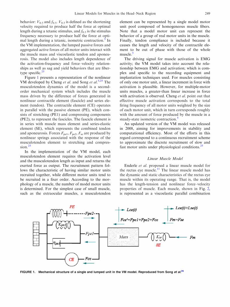
Figure 1 presents a representation of the nonlinearVM developed by Cheng et al. and Song et al.5,25 Themusculotendon dynamics of the model is a second-order mechanical system which includes the musclemass driven by the difference of forces generated innonlinear contractile element (fascicle) and series ele-ment (tendon). The contractile element (CE) operatesin parallel with the passive element (PE), which con-sists of stretching (PE1) and compressing components(PE2), to represent the fascicles. The fascicle element isin series with muscle mass element and series-elasticelement (SE), which represents the combined tendonand aponeurosis. Forces Fpe1, Fpe2, Fse are produced bynonlinear springs associated with the response of themusculotendon element to stretching and compres-sion.25

In the implementation of the VM model, eachmusculotendon element requires the activation leveland the musculotendon length as input and returns theexerted force as output. The recruitment pattern fol-lows the characteristic of having similar motor unitsrecruited together, while different motor units tend tobe recruited in a fixer order. According to the mor-phology of a muscle, the number of model motor unitsis determined. For the simplest case of small muscle,such as the extraocular muscles, a musculotendon

element can be represented by a single model motorunit pool composed of homogeneous muscle fibers.Note that a model motor unit can represent thebehavior of a group of real motor units in the muscle.Finally, tendon compliance is included because itcauses the length and velocity of the contractile ele-ment to be out of phase with those of the wholemuscle.5

The driving signal for muscle activation is EMGactivity; the VM model takes into account the rela-tionship between EMG and activation; which is com-plex and specific to the recording equipment andimplantation techniques used. For muscles consistingof only one motor unit, a linear increment in force withactivation is plausible. However, for multiple-motorunits muscles, a greater-than linear increase in forcewith activation is observed. Cheng et al. point out thateffective muscle activation corresponds to the totalfiring frequency of all motor units weighted by the sizeof each motor unit, which in turn corresponds roughlywith the amount of force produced by the muscle in asteady-state isometric contraction.5

An updated version of the VM model was releasedin 2008, aiming for improvements in stability andcomputational efficiency. Most of the efforts in thisregard correspond to a continuous recruitment schemeto approximate the discrete recruitment of slow andfast motor units under physiological conditions.25

Linear Muscle Model

Enderle et al. proposed a linear muscle model forthe rectus eye muscle.11 The linear muscle model hasthe dynamic and static characteristics of the rectus eyemuscle within its operating range. That is, the modelhas the length-tension and nonlinear force–velocityproperties of muscle. Each muscle, shown in Fig. 2,is represented as a viscoelastic parallel combination

FIGURE 1. Mechanical structure of a single and lumped unit in the VM model. Reproduced from Song et al.25

Linear Models for Muscles in the Head–Neck Region 249

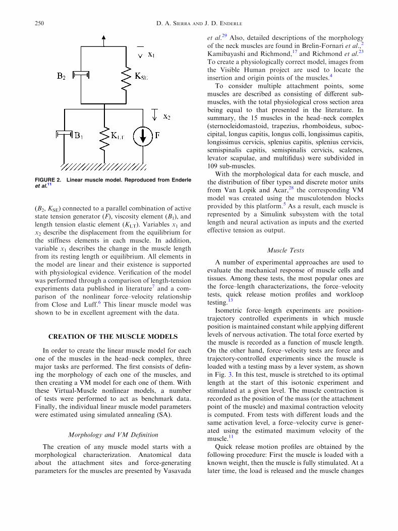
(B2, KSE) connected to a parallel combination of activestate tension generator (F), viscosity element (B1), andlength tension elastic element (KLT). Variables x1 andx2 describe the displacement from the equilibrium forthe stiffness elements in each muscle. In addition,variable x1 describes the change in the muscle lengthfrom its resting length or equilibrium. All elements inthe model are linear and their existence is supportedwith physiological evidence. Verification of the modelwas performed through a comparison of length-tensionexperiments data published in literature7 and a com-parison of the nonlinear force–velocity relationshipfrom Close and Luff.6 This linear muscle model wasshown to be in excellent agreement with the data.

CREATION OF THE MUSCLE MODELS

In order to create the linear muscle model for eachone of the muscles in the head–neck complex, threemajor tasks are performed. The first consists of defin-ing the morphology of each one of the muscles, andthen creating a VM model for each one of them. Withthese Virtual-Muscle nonlinear models, a numberof tests were performed to act as benchmark data.Finally, the individual linear muscle model parameterswere estimated using simulated annealing (SA).

Morphology and VM Definition

The creation of any muscle model starts with amorphological characterization. Anatomical dataabout the attachment sites and force-generatingparameters for the muscles are presented by Vasavada

et al.29 Also, detailed descriptions of the morphologyof the neck muscles are found in Brelin-Fornari et al.,2

Kamibayashi and Richmond,17 and Richmond et al.23

To create a physiologically correct model, images fromthe Visible Human project are used to locate theinsertion and origin points of the muscles.4

To consider multiple attachment points, somemuscles are described as consisting of different sub-muscles, with the total physiological cross section areabeing equal to that presented in the literature. Insummary, the 15 muscles in the head–neck complex(sternocleidomastoid, trapezius, rhomboideus, suboc-cipital, longus capitis, longus colli, longissimus capitis,longissimus cervicis, splenius capitis, splenius cervicis,semispinalis capitis, semispinalis cervicis, scalenes,levator scapulae, and multifidus) were subdivided in109 sub-muscles.

With the morphological data for each muscle, andthe distribution of fiber types and discrete motor unitsfrom Van Lopik and Acar,28 the corresponding VMmodel was created using the musculotendon blocksprovided by this platform.5 As a result, each muscle isrepresented by a Simulink subsystem with the totallength and neural activation as inputs and the exertedeffective tension as output.

Muscle Tests

A number of experimental approaches are used toevaluate the mechanical response of muscle cells andtissues. Among these tests, the most popular ones arethe force–length characterizations, the force–velocitytests, quick release motion profiles and worklooptesting.13

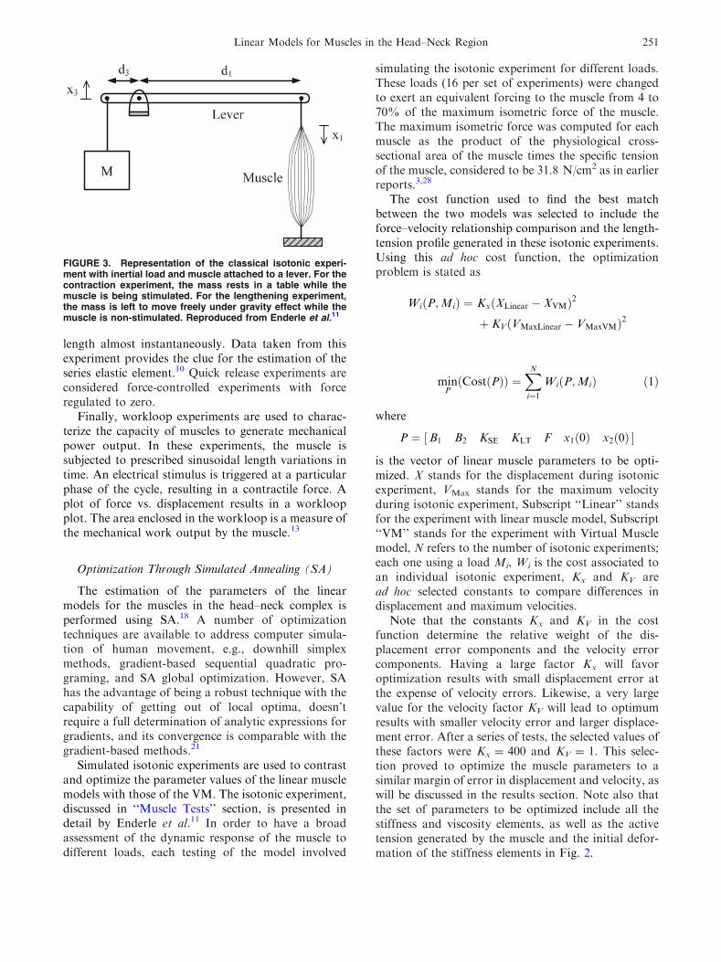
Isometric force–length experiments are position-trajectory controlled experiments in which muscleposition is maintained constant while applying differentlevels of nervous activation. The total force exerted bythe muscle is recorded as a function of muscle length.On the other hand, force–velocity tests are force andtrajectory-controlled experiments since the muscle isloaded with a testing mass by a lever system, as shownin Fig. 3. In this test, muscle is stretched to its optimallength at the start of this isotonic experiment andstimulated at a given level. The muscle contraction isrecorded as the position of the mass (or the attachmentpoint of the muscle) and maximal contraction velocityis computed. From tests with different loads and thesame activation level, a force–velocity curve is gener-ated using the estimated maximum velocity of themuscle.11

Quick release motion profiles are obtained by thefollowing procedure: First the muscle is loaded with aknown weight, then the muscle is fully stimulated. At alater time, the load is released and the muscle changes

FIGURE 2. Linear muscle model. Reproduced from Enderleet al.11

D. A. SIERRA AND J. D. ENDERLE250

length almost instantaneously. Data taken from thisexperiment provides the clue for the estimation of theseries elastic element.10 Quick release experiments areconsidered force-controlled experiments with forceregulated to zero.

Finally, workloop experiments are used to charac-terize the capacity of muscles to generate mechanicalpower output. In these experiments, the muscle issubjected to prescribed sinusoidal length variations intime. An electrical stimulus is triggered at a particularphase of the cycle, resulting in a contractile force. Aplot of force vs. displacement results in a workloopplot. The area enclosed in the workloop is a measure ofthe mechanical work output by the muscle.13

Optimization Through Simulated Annealing (SA)

The estimation of the parameters of the linearmodels for the muscles in the head–neck complex isperformed using SA.18 A number of optimizationtechniques are available to address computer simula-tion of human movement, e.g., downhill simplexmethods, gradient-based sequential quadratic pro-graming, and SA global optimization. However, SAhas the advantage of being a robust technique with thecapability of getting out of local optima, doesn’trequire a full determination of analytic expressions forgradients, and its convergence is comparable with thegradient-based methods.21

Simulated isotonic experiments are used to contrastand optimize the parameter values of the linear musclemodels with those of the VM. The isotonic experiment,discussed in ‘‘Muscle Tests’’ section, is presented indetail by Enderle et al.11 In order to have a broadassessment of the dynamic response of the muscle todifferent loads, each testing of the model involved

simulating the isotonic experiment for different loads.These loads (16 per set of experiments) were changedto exert an equivalent forcing to the muscle from 4 to70% of the maximum isometric force of the muscle.The maximum isometric force was computed for eachmuscle as the product of the physiological cross-sectional area of the muscle times the specific tensionof the muscle, considered to be 31.8 N/cm2 as in earlierreports.3,28

The cost function used to find the best matchbetween the two models was selected to include theforce–velocity relationship comparison and the length-tension profile generated in these isotonic experiments.Using this ad hoc cost function, the optimizationproblem is stated as

Wi P;Mið Þ ¼ Kx XLinear � XVMð Þ2

þ KV VMaxLinear � VMaxVMð Þ2

minP

Cost Pð Þð Þ ¼XN

i¼1Wi P;Mið Þ ð1Þ

where

P ¼ B1 B2 KSE KLT F x1 0ð Þ x2 0ð Þ½ �

is the vector of linear muscle parameters to be opti-mized. X stands for the displacement during isotonicexperiment, VMax stands for the maximum velocityduring isotonic experiment, Subscript ‘‘Linear’’ standsfor the experiment with linear muscle model, Subscript‘‘VM’’ stands for the experiment with Virtual Musclemodel, N refers to the number of isotonic experiments;each one using a load Mi, Wi is the cost associated toan individual isotonic experiment, Kx and KV aread hoc selected constants to compare differences indisplacement and maximum velocities.

Note that the constants Kx and KV in the costfunction determine the relative weight of the dis-placement error components and the velocity errorcomponents. Having a large factor Kx will favoroptimization results with small displacement error atthe expense of velocity errors. Likewise, a very largevalue for the velocity factor KV will lead to optimumresults with smaller velocity error and larger displace-ment error. After a series of tests, the selected values ofthese factors were Kx = 400 and KV = 1. This selec-tion proved to optimize the muscle parameters to asimilar margin of error in displacement and velocity, aswill be discussed in the results section. Note also thatthe set of parameters to be optimized include all thestiffness and viscosity elements, as well as the activetension generated by the muscle and the initial defor-mation of the stiffness elements in Fig. 2.

FIGURE 3. Representation of the classical isotonic experi-ment with inertial load and muscle attached to a lever. For thecontraction experiment, the mass rests in a table while themuscle is being stimulated. For the lengthening experiment,the mass is left to move freely under gravity effect while themuscle is non-stimulated. Reproduced from Enderle et al.11

Linear Models for Muscles in the Head–Neck Region 251

SA implementation

The optimization of SA was performed in Matlabusing the function created by Vandekerckhove.27 Thefollowing steps are performed tofind optimal parameters:

(1) Select set of parameter values as initial guessP0.

(2) Define a generator of random parameters.This function will determine how the searchwill select new guessed parameters in theneighborhood of the current solution. In eachstep, only one parameter value is changed.For the problem at hand, the new parameterestimative was the current one plus a randomnumber generated from a normal distributionwith standard deviation 10% of the initialguess for the parameter. Let be j the randomlypicked parameter to change, the new value forthis parameter will be:

PNew jð Þ ¼ PCurrent jð Þ þ 0:1P0 jð Þ �Randn 0; 1ð Þð2Þ

where PCurrent is the last set of optimalparameters, and Randn(0,1) is a randomnumber with normal distribution of mean 0and standard deviation 1.

(3) Define a cooling schedule to generate a newtemperature from the previous one. Thecooling schedule was selected to be 0.8T. Aninitial temperature of T = 1 is set and a finaltemperature of T = 1e�8 is used to define theend of the search (this allows for 83 temper-ature levels to be evaluated).

(4) For each temperature, a number of tries looksfor new parameter values using the generatorfunction and using the current parameters.For each set of new parameters, the costfunction is evaluated and compared with thecurrent optimum cost.

(a) IfDCost ” Cost(PNew) � Cost(PCurrent) £ 0,the new set of parameters is accepted asthe new optimal set (PCurrent ‹ PNew),and a success is counted.

(b) If DCost> 0, the new set of parameters isaccepted as the new optimal in a probabi-listic way. The probability that this newconfiguration is accepted as new optimal(success) is P DCostð Þ¼ expð�DCost=KTÞ.In analogy with statistical mechanics, K iscalled the Boltzmann’s Constant, but forsimplicity K is set to 1.

(c) The search in each temperature level canbe over by either reaching a maximumnumber of tries per temperature level or

reaching a maximum number of suc-cesses per temperature level.

(5) A number of conditions may end the globalsearch:

(a) The temperature reaches a level belowthe final temperature.

(b) A maximum number of consecutiverejections have been reached (defined astries with DCost> 0 and not accepted assuccesses). Each time a DCost £ 0 isobtained, the counter of consecutiverejections is reset.

(c) The cost function reaches a level smallenough to finalize the optimization.

RESULTS

The use of SA allows the estimation of the param-eters for the different muscles in the head and neckcomplex. However, since experimental data is availablefor the rectus eye muscle, the estimation of a non-linearmodel for this and the optimization to find the linearparameters of this muscle is presented first.

Rectus Eye Muscle Modeling Results

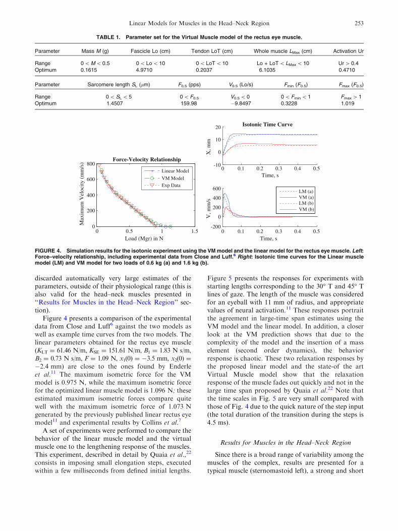
In order to prove the suitability of the methodol-ogy, the experimental data from Collins et al.7 andClose and Luff6 were used to estimate a VM model ofthe rectus eye muscle. In this case, the set of parame-ters to be optimized are the morphological and fibertype parameters required to implement the VMmodel.5 The muscle was modeled with a single discretemotor unit representing the dynamics of the wholemuscle, as suggested by Cheng et al. for small muscleswith primarily one type of muscle fiber.5 The param-eters of the optimized VM model (both morphologicaland fiber type parameters) are presented in Table 1,which correspond to values in the physiological rangefor the rectus eye muscle. To avoid sets of parameterswith non-physiological correspondence (e.g., negativelengths), the subspace of search for the parameters wasrestrained as presented in Table 1; sets of parametersoutside this subspace were discarded assigning a verylarge cost.

This VM model was then used to find the linearparameters that model the muscle. Isotonic experi-ments with a range of loads were simulated and theoptimization process explained above was carried out.In the case of linear parameters search, the onlyrestriction imposed to the search subspace was to havepositive values in the parameters; the SA algorithm

D. A. SIERRA AND J. D. ENDERLE252

discarded automatically very large estimates of theparameters, outside of their physiological range (this isalso valid for the head–neck muscles presented in‘‘Results for Muscles in the Head–Neck Region’’ sec-tion).

Figure 4 presents a comparison of the experimentaldata from Close and Luff6 against the two models aswell as example time curves from the two models. Thelinear parameters obtained for the rectus eye muscle(KLT = 61.46 N/m, KSE = 151.61 N/m, B1 = 1.83 N s/m,B2 = 0.73 N s/m, F = 1.09 N, x1(0) = �3.5 mm, x2(0) =

�2.4 mm) are close to the ones found by Enderleet al.11 The maximum isometric force for the VMmodel is 0.975 N, while the maximum isometric forcefor the optimized linear muscle model is 1.096 N; theseestimated maximum isometric forces compare quitewell with the maximum isometric force of 1.073 Ngenerated by the previously published linear rectus eyemodel11 and experimental results by Collins et al.7

A set of experiments were performed to compare thebehavior of the linear muscle model and the virtualmuscle one to the lengthening response of the muscles.This experiment, described in detail by Quaia et al.,22

consists in imposing small elongation steps, executedwithin a few milliseconds from defined initial lengths.

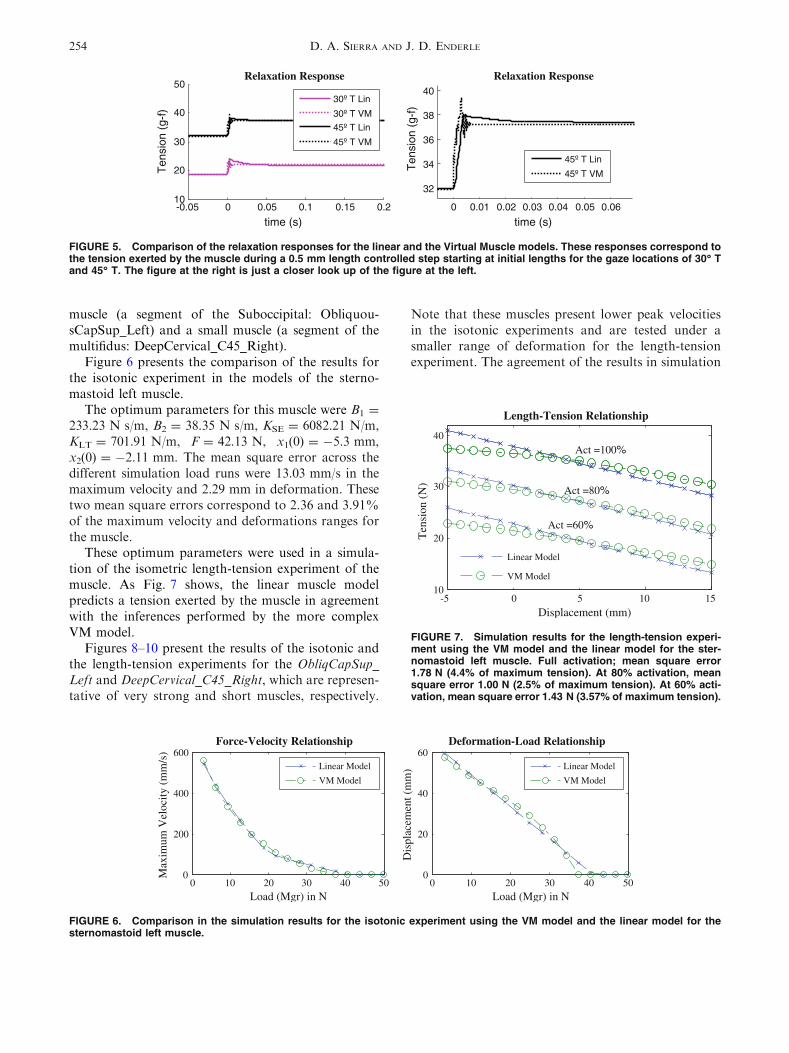
Figure 5 presents the responses for experiments withstarting lengths corresponding to the 30� T and 45� Tlines of gaze. The length of the muscle was consideredfor an eyeball with 11 mm of radius, and appropriatevalues of neural activation.11 These responses portraitthe agreement in large-time span estimates using theVM model and the linear model. In addition, a closerlook at the VM prediction shows that due to thecomplexity of the model and the insertion of a masselement (second order dynamics), the behaviorresponse is chaotic. These two relaxation responses bythe proposed linear model and the state-of the artVirtual Muscle model show that the relaxationresponse of the muscle fades out quickly and not in thelarge time span proposed by Quaia et al.22 Note thatthe time scales in Fig. 5 are very small compared withthose of Fig. 4 due to the quick nature of the step input(the total duration of the transition during the steps is4.5 ms).

Results for Muscles in the Head–Neck Region

Since there is a broad range of variability among themuscles of the complex, results are presented for atypical muscle (sternomastoid left), a strong and short

TABLE 1. Parameter set for the Virtual Muscle model of the rectus eye muscle.

Parameter Mass M (g) Fascicle Lo (cm) Tendon LoT (cm) Whole muscle LMax (cm) Activation Ur

Range 0 < M < 0.5 0 < Lo < 10 0 < LoT < 10 Lo + LoT < LMax < 10 Ur > 0.4

Optimum 0.1615 4.9710 0.2037 6.1035 0.4710

Parameter Sarcomere length SL (lm) F0.5 (pps) V0.5 (Lo/s) Fmin (F0.5) Fmax (F0.5)

Range 0 < SL < 5 0 < F0.5 V0.5 < 0 0 < Fmin < 1 Fmax > 1

Optimum 1.4507 159.98 �9.8497 0.3228 1.019

0 0.5 1 1.50

200

400

600

800

Load (Mgr) in N

Max

imum

Vel

ocity

(m

m/s

) Force-Velocity Relationship

Linear Model

VM ModelExp Data

0 0.1 0.2 0.3 0.4 0.5-10

0

10

20

Time, s

X, m

m

Isotonic Time Curve

0 0.1 0.2 0.3 0.4 0.5-200

0

200

400

600

Time, s

V, m

m/s

LM (a)VM (a)LM (b)VM (b)

FIGURE 4. Simulation results for the isotonic experiment using the VM model and the linear model for the rectus eye muscle. Left:Force–velocity relationship, including experimental data from Close and Luff.6 Right: Isotonic time curves for the Linear musclemodel (LM) and VM model for two loads of 0.6 kg (a) and 1.6 kg (b).

Linear Models for Muscles in the Head–Neck Region 253

muscle (a segment of the Suboccipital: Obliquou-sCapSup_Left) and a small muscle (a segment of themultifidus: DeepCervical_C45_Right).

Figure 6 presents the comparison of the results forthe isotonic experiment in the models of the sterno-mastoid left muscle.

The optimum parameters for this muscle were B1 =

233.23 N s/m, B2 = 38.35 N s/m, KSE = 6082.21 N/m,KLT = 701.91 N/m, F = 42.13 N, x1(0) = �5.3 mm,x2(0) = �2.11 mm. The mean square error across thedifferent simulation load runs were 13.03 mm/s in themaximum velocity and 2.29 mm in deformation. Thesetwo mean square errors correspond to 2.36 and 3.91%of the maximum velocity and deformations ranges forthe muscle.

These optimum parameters were used in a simula-tion of the isometric length-tension experiment of themuscle. As Fig. 7 shows, the linear muscle modelpredicts a tension exerted by the muscle in agreementwith the inferences performed by the more complexVM model.

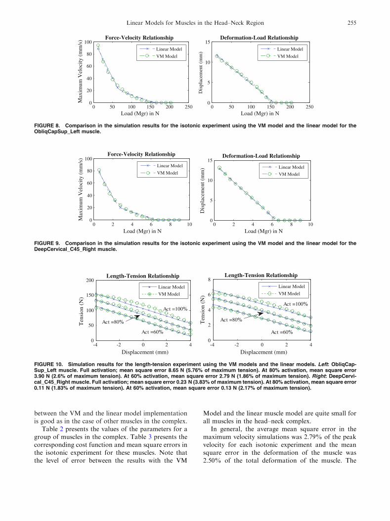
Figures 8–10 present the results of the isotonic andthe length-tension experiments for the ObliqCapSup_Left and DeepCervical_C45_Right, which are represen-tative of very strong and short muscles, respectively.

Note that these muscles present lower peak velocitiesin the isotonic experiments and are tested under asmaller range of deformation for the length-tensionexperiment. The agreement of the results in simulation

-0.05 0 0.05 0.1 0.15 0.210

20

30

40

50

time (s)

Ten

sion

(g-

f)

Relaxation Response

30º T Lin

30º T VM

45º T Lin

45º T VM

0 0.01 0.02 0.03 0.04 0.05 0.06

32

34

36

38

40

time (s)

Ten

sion

(g-

f)

Relaxation Response

45º T Lin

45º T VM

FIGURE 5. Comparison of the relaxation responses for the linear and the Virtual Muscle models. These responses correspond tothe tension exerted by the muscle during a 0.5 mm length controlled step starting at initial lengths for the gaze locations of 30� Tand 45� T. The figure at the right is just a closer look up of the figure at the left.

0 10 20 30 40 500

200

400

600

Load (Mgr) in N

Max

imum

Vel

ocity

(m

m/s

)

Force-Velocity Relationship

Linear Model

VM Model

0 10 20 30 40 500

20

40

60

Load (Mgr) in N

Dis

plac

emen

t (m

m)

Deformation-Load Relationship

Linear Model

VM Model

FIGURE 6. Comparison in the simulation results for the isotonic experiment using the VM model and the linear model for thesternomastoid left muscle.

-5 0 5 10 1510

20

30

40

Displacement (mm)

Ten

sion

(N

)Length-Tension Relationship

Act =100%

Act =80%

Act =60%

Linear Model

VM Model

FIGURE 7. Simulation results for the length-tension experi-ment using the VM model and the linear model for the ster-nomastoid left muscle. Full activation; mean square error1.78 N (4.4% of maximum tension). At 80% activation, meansquare error 1.00 N (2.5% of maximum tension). At 60% acti-vation, mean square error 1.43 N (3.57% of maximum tension).

D. A. SIERRA AND J. D. ENDERLE254

between the VM and the linear model implementationis good as in the case of other muscles in the complex.

Table 2 presents the values of the parameters for agroup of muscles in the complex. Table 3 presents thecorresponding cost function and mean square errors inthe isotonic experiment for these muscles. Note thatthe level of error between the results with the VM

Model and the linear muscle model are quite small forall muscles in the head–neck complex.

In general, the average mean square error in themaximum velocity simulations was 2.79% of the peakvelocity for each isotonic experiment and the meansquare error in the deformation of the muscle was2.50% of the total deformation of the muscle. The

0 50 100 150 200 2500

20

40

60

80

100

Load (Mgr) in N

Max

imum

Vel

ocity

(m

m/s

) Force-Velocity Relationship

Linear Model

VM Model

0 50 100 150 200 2500

5

10

15

Load (Mgr) in N

Dis

plac

emen

t (m

m)

Deformation-Load Relationship

Linear Model

VM Model

FIGURE 8. Comparison in the simulation results for the isotonic experiment using the VM model and the linear model for theObliqCapSup_Left muscle.

0 2 4 6 8 100

20

40

60

80

100

Load (Mgr) in N

Max

imum

Vel

ocity

(m

m/s

)

Force-Velocity Relationship

Linear Model

VM Model

0 2 4 6 8 100

5

10

15

Load (Mgr) in N

Dis

plac

emen

t (m

m)

Deformation-Load Relationship

Linear Model

VM Model

FIGURE 9. Comparison in the simulation results for the isotonic experiment using the VM model and the linear model for theDeepCervical_C45_Right muscle.

-4 -2 0 2 40

50

100

150

200

Displacement (mm)

Ten

sion

(N

)

Length-Tension Relationship

Act =60%

Act =80%

Act =100%

Linear Model

VM Model

-4 -2 0 2 40

2

4

6

8

Displacement (mm)

Ten

sion

(N

)

Length-Tension Relationship

Act =60%

Act =80%

Act =100%

Linear Model

VM Model

FIGURE 10. Simulation results for the length-tension experiment using the VM models and the linear models. Left: ObliqCap-Sup_Left muscle. Full activation; mean square error 8.65 N (5.76% of maximum tension). At 80% activation, mean square error3.90 N (2.6% of maximum tension). At 60% activation, mean square error 2.79 N (1.86% of maximum tension). Right: DeepCervi-cal_C45_Right muscle. Full activation; mean square error 0.23 N (3.83% of maximum tension). At 80% activation, mean square error0.11 N (1.83% of maximum tension). At 60% activation, mean square error 0.13 N (2.17% of maximum tension).

Linear Models for Muscles in the Head–Neck Region 255

maximum isometric force was computed for each lin-ear muscle model and compared with the product ofthe physiological cross-sectional area of the muscletimes the specific tension of the muscle, defined previ-ously for the VM model implementation. Estimates ofthe maximal isometric force using the optimized linearmodels ranged 101.38 ± 2.18% (Mean ± SD) fromtheir associated physiological estimates.

DISCUSSION

Implementing physiological systems models pre-sents a challenge of balancing the level of complexityof the model with its use. Very complex and precisemodels can be formulated at the expense of morecomputational power. When incorporating musclemodels into large-scale systems, such as the head–neckcomplex, the objective is to use the simplest model,with the fewest parameters, that has the properties ofthe experimental data.11,30 Here, we show the feasi-bility of using a linear muscle model with only fivelumped parameters to represent the dynamics ofmuscles in the head and neck complex. Features of themuscle are translated to VM and then to the linearmuscle model.

The obtained parameters for the linear musclemodels allow the duplication of the isotonic experi-ment and length tension experiment, considered themost important properties which describe muscle.30

Simulation of these experiments using the proposedlinear model provides results with a good degree ofaccuracy with respect to a broadly accepted and usedmodel (VM, developed by Cheng et al. and Songet al.5,25). Yet the VM model considers a greater scopeof characteristics for the muscle dynamics, includingthe neural activation modulation, the complexity of themodel is high, added with the nonlinear characteristicsin it that prevents from using classical techniques toanalyze them.

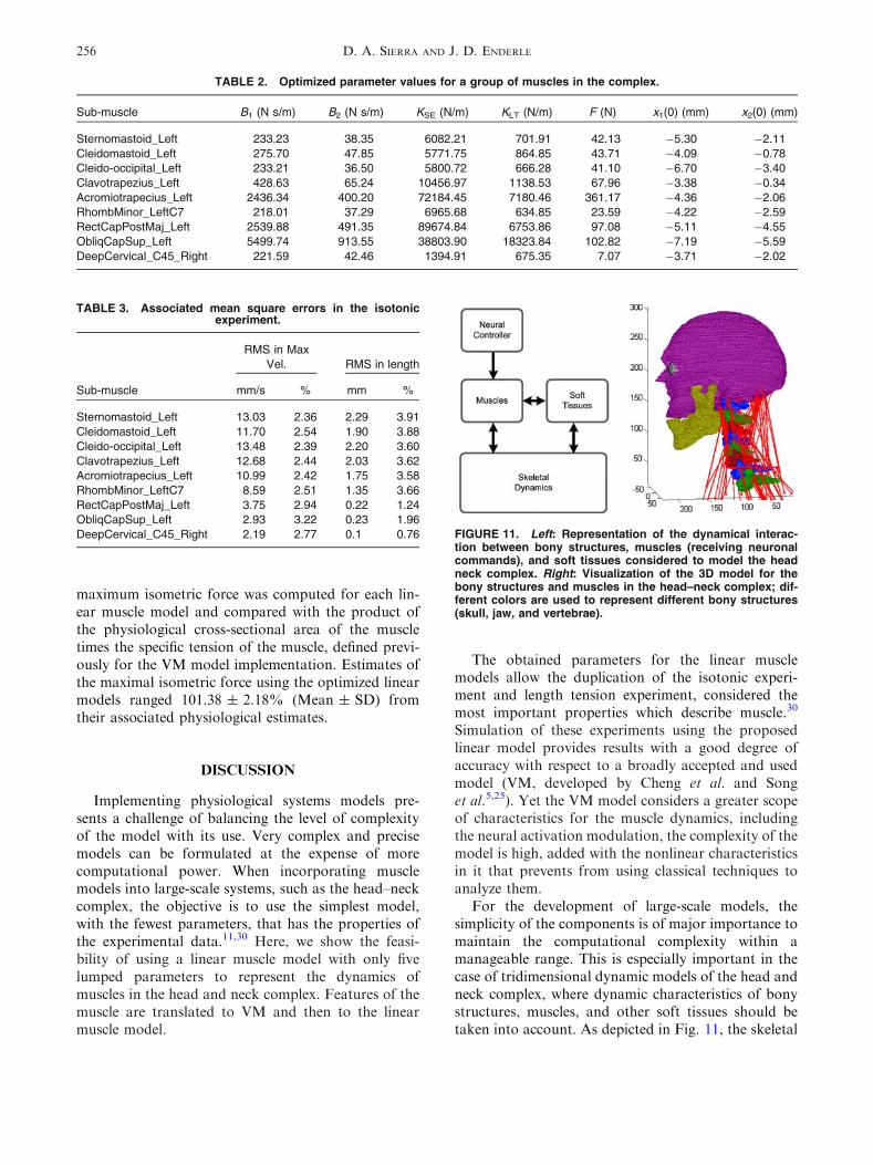
For the development of large-scale models, thesimplicity of the components is of major importance tomaintain the computational complexity within amanageable range. This is especially important in thecase of tridimensional dynamic models of the head andneck complex, where dynamic characteristics of bonystructures, muscles, and other soft tissues should betaken into account. As depicted in Fig. 11, the skeletal

TABLE 2. Optimized parameter values for a group of muscles in the complex.

Sub-muscle B1 (N s/m) B2 (N s/m) KSE (N/m) KLT (N/m) F (N) x1(0) (mm) x2(0) (mm)

Sternomastoid_Left 233.23 38.35 6082.21 701.91 42.13 �5.30 �2.11

Cleidomastoid_Left 275.70 47.85 5771.75 864.85 43.71 �4.09 �0.78

Cleido-occipital_Left 233.21 36.50 5800.72 666.28 41.10 �6.70 �3.40

Clavotrapezius_Left 428.63 65.24 10456.97 1138.53 67.96 �3.38 �0.34

Acromiotrapecius_Left 2436.34 400.20 72184.45 7180.46 361.17 �4.36 �2.06

RhombMinor_LeftC7 218.01 37.29 6965.68 634.85 23.59 �4.22 �2.59

RectCapPostMaj_Left 2539.88 491.35 89674.84 6753.86 97.08 �5.11 �4.55

ObliqCapSup_Left 5499.74 913.55 38803.90 18323.84 102.82 �7.19 �5.59

DeepCervical_C45_Right 221.59 42.46 1394.91 675.35 7.07 �3.71 �2.02

TABLE 3. Associated mean square errors in the isotonicexperiment.

Sub-muscle

RMS in Max

Vel. RMS in length

mm/s % mm %

Sternomastoid_Left 13.03 2.36 2.29 3.91

Cleidomastoid_Left 11.70 2.54 1.90 3.88

Cleido-occipital_Left 13.48 2.39 2.20 3.60

Clavotrapezius_Left 12.68 2.44 2.03 3.62

Acromiotrapecius_Left 10.99 2.42 1.75 3.58

RhombMinor_LeftC7 8.59 2.51 1.35 3.66

RectCapPostMaj_Left 3.75 2.94 0.22 1.24

ObliqCapSup_Left 2.93 3.22 0.23 1.96

DeepCervical_C45_Right 2.19 2.77 0.1 0.76 FIGURE 11. Left: Representation of the dynamical interac-tion between bony structures, muscles (receiving neuronalcommands), and soft tissues considered to model the headneck complex. Right: Visualization of the 3D model for thebony structures and muscles in the head–neck complex; dif-ferent colors are used to represent different bony structures(skull, jaw, and vertebrae).

D. A. SIERRA AND J. D. ENDERLE256

dynamics depends on the forces and momenta exertedby muscles and soft tissues, with the muscles being theonly active elements in the system that receive theneuronal commands. Using linear muscle models forthe head–neck region allows the reduction of thecomplexity on the model while approximating the mostimportant dynamic properties of the full system. Thesemodels will be useful when integrated head–neck andeye dynamic model are in place to study the neuralcontrol of time-optimal gaze shifts.

CONCLUSION

A linear homeomorphic muscle model was shown towork approximating non-linear dynamics for musclesin the head–neck complex. Simulated annealing provedto be a suitable approach to find optimum linearparameters for these muscles, with the advantage ofnot needing analytic definition of gradients andavoiding local minima.

Having linear muscle models with complex dynamicbehavior like those presented in the isotonic experi-ment and under length-tension experiments allows forthe simplification of human movement models. Inparticular, the parameters obtained for muscles in thehead–neck complex are used in a 3D dynamic com-puter model for the movement of the head–neckcomplex, to be presented in a future paper, and aimedto study the neural control of the complex during fasteye and head movements such as saccades and gazeshifts. The incorporation of modeling strategies foreach one of the components of the complex such asbony structures, soft tissues, and muscles aims to getmore dependable inferences about the dynamics of thefull complex.

The current approach to find the parameters of thelinear model uses predictions from the VM model.Better models and estimates can be drawn if experi-mental tests are performed from real muscles. With theimplementation of a setup to repeat isotonic and iso-metric experiments, a good deal of data will be avail-able for this purpose and the improvement of thesubsequent models.

REFERENCES

1Bizzi, E., R. E. Kalil, and V. Tagliasco. Eye-head coordi-nation in monkeys: evidence for centrally patterned orga-nization. Science 173:452–454, 1971.2Brelin-Fornari, J., P. Shah, and M. El-Sayed. Physicallycorrelated muscle activation for a human head and neckcomputational model. Comput. Methods Biomech. Biomed.Eng. 8:191–199, 2005.

3Brown, I. E., S. H. Scott, and G. E. Loeb. Mechanics offeline soleus: II design and validation of a mathematicalmodel. J. Muscle Res. Cell Motil. 17:221–233, 1996.4Chang, Y., P. Coddington, and K. Hutchens. The NPAC/OLDA Visible Human Viewer. Adelaide, Australia:Computer Science Department, Adelaide University.www.dhpc.adelaide.edu.au/projects/vishuman2/. Accessed11 July 2007.5Cheng, E. J., I. E. Brown, and G. E. Loeb. Virtual muscle:a computational approach to understanding the effects ofmuscle properties on motor control. J. Neurosci. Methods101:117–130, 2000.6Close, R. I., and A. R. Luff. Dynamic properties of inferiorrectus muscle of the rat. J. Physiol. 236:259–270, 1974.7Collins, C. C., D. O’Meara, and A. B. Scott. Muscle ten-sion during unrestrained human eye movements. J. Phys-iol. 245:351–369, 1975.8Enderle, J. D. A Physiological Neural Network for Sacc-adic Eye Movement Control. Report AL/AO-TR-1994-0023 prepared for Armstrong Laboratory AL/AOCFOBrooks AFRB, TX, 1994.9Enderle, J. D. Neural control of saccades. Prog. Brain Res.140:21–49, 2002.

10Enderle, J. D., J. D. Bronzino, and S. M. Blanchard.Introduction to Biomedical Engineering, vol. xxi. Amster-dam: Elsevier Academic Press, 1118 pp., 2005.

11Enderle, J. D., E. J. Engelken, and R. N. Stiles. A com-parison of static and dynamic characteristics between rec-tus eye muscle and linear muscle model predictions. IEEETrans. Biomed. Eng. 38:1235–1245, 1991.

12Enderle, J. D., and J. W. Wolfe. Time-optimal control ofsaccadic eye movements. IEEE Trans. Biomed. Eng. 34:43–55, 1987.

13Farahat, W., and H. Herr. An apparatus for character-ization and control of isolated muscle. IEEE Trans. NeuralSyst. Rehabil. Eng. 13:473–481, 2005.

14Freedman, E. G. Coordination of the eyes and head duringvisual orienting. Exp. Brain Res. 190:369–387, 2008.

15Freedman, E. G., and D. L. Sparks. Eye-head coordinationduring head-unrestrained gaze shifts in rhesus monkeys.J. Neurophysiol. 77:2328–2348, 1997.

16Hannaford, B. Control of Fast Movement: Human HeadRotation. PhD dissertation, University of California,Berkeley, 1985.

17Kamibayashi, L. K., and F. J. Richmond. Morphometry ofhuman neck muscles. Spine 23:1314–1323, 1998.

18Kirkpatrick, S., C. D. Gelatt, Jr., and M. P. Vecchi.Optimization by simulated annealing. Science 220:671–680,1983.

19Lestienne, F., P. P. Vidal, and A. Berthoz. Gaze changingbehaviour in head restrained monkey. Exp. Brain Res.53:349–356, 1984.

20Morasso, P., G. Sandini, V. Tagliasco, and R. Zaccaria.Control strategies in the eye-head coordination system.IEEE Trans. Syst. Man Cybern. 7:639–651, 1977.

21Neptune, R. R. Optimization algorithm performance indetermining optimal controls in human movement analy-ses. J. Biomech. Eng. 121:249–252, 1999.

22Quaia, C., H. S. Ying, A. M. Nichols, and L. M. Optican.The viscoelastic properties of passive eye muscle in pri-mates. I. Static and step responses. PLoS One 4:e4850,2009.

23Richmond, F. J., K. Singh, and B. D. Corneil. Neckmuscles in the rhesus monkey. I. Muscle morphometry andhistochemistry. J. Neurophysiol. 86:1717–1728, 2001.

Linear Models for Muscles in the Head–Neck Region 257

24Scudder, C. A., C. S. Kaneko, and A. F. Fuchs. Thebrainstem burst generator for saccadic eye movements: amodern synthesis. Exp. Brain Res. 142:439–462, 2002.

25Song, D., G. Raphael, N. Lan, and G. E. Loeb. Compu-tationally efficient models of neuromuscular recruitmentand mechanics. J. Neural Eng. 5:175–184, 2008.

26Sylvestre, P. A., and K. E. Cullen. Premotor correlatesof integrated feedback control for eye-head gaze shifts.J. Neurosci. 26:4922–4929, 2006.

27Vandekerckhove, J. General Simulated Annealing Algo-rithm, 2006. http://www.mathworks.com/matlabcentral/fileexchange/10548. Accessed 14 July 2008.

28Van Lopik, D. W., and M. Acar. Development of a multi-body computational model of human head and neck. Proc.

Inst. Mech. Eng. Part K: J. Multi-body Dyn. 221:175–197,2007.

29Vasavada, A. N., S. Li, and S. L. Delp. Influence of musclemorphometry and moment arms on the moment-generatingcapacity of human neck muscles. Spine 23:412–422, 1998.

30Zajac, F. E. Muscle and tendon: properties, models, scal-ing, and application to biomechanics and motor control.Crit. Rev. Biomed. Eng. 17:359–411, 1989.

31Zangemeister, W. H., A. C. Arlt, and S. Lehman. Sensi-tivity functions of a human head movement model. Med.Eng. Phys. 16:163–170, 1994.

32Zangemeister, W. H., L. Stark, O. Meienberg, andT. Waite. Neural control of head rotation: electromyo-graphic evidence. J. Neurol. Sci. 55:1–14, 1982.

D. A. SIERRA AND J. D. ENDERLE258