Moment and Memory Properties of LinearConditional Heteroscedasticity Models,and a New ModelJames DAVIDSON

Cardiff Business School, Cardiff CF10 3EU, U.K. (davidsonje@cardiff.ac.uk)

This article analyses the statistical properties of that general class of conditional heteroscedasticity modelsin which the conditional variance is a linear function of squared lags of the process. GARCH, IGARCH,FIGARCH, and a newly proposed generalization, the HYGARCH model, belong to this class. Conditionsare derived for the existence of second and fourth moments, and for the limited memory condition ofnear-epoch dependence. The HYGARCH model is applied to 10 daily dollar exchange rates, and also todata for Asian exchange rates over the 1997 crisis period. In the latter case, the model exhibits notablestability across the pre-crisis and post-crisis periods.

KEY WORDS: ARCH(in� nity); FIGARCH; Hyperbolic lag; Near-epoch dependence; Exchange rate.

1. INTRODUCTION

Many variants of Engle’s (1982) ARCH model of conditionalvolatility have been proposed, including GARCH (Bollerslev1986), IGARCH (Engle and Bollerslev 1986), and FIGARCH(Baillie, Bollerslev, and Mikkelsen 1996; Ding and Granger1996). All of these models, and many other cases that might bedevised, fall into the class in which the conditional variance attime t is an in� nite moving average of the squared realizationsof the series up to time t ¡ 1: Formally, let

ut D ¾tet; (1)

where ¾t > 0, et » iid.0; 1/, and

¾ 2t D ! C

1X

iD1

µiu2t¡i; µi ¸ 0 for all i; (2)

where µi are lag coef� cients typically depending on a smallnumber of underlying parameters. By adding an error term,vt D u2

t ¡ ¾ 2t , to both sides, (2) can be viewed as an AR(1) in

the squared series, and hence is commonlycalled an ARCH(1)model.

In the well-known case of the GARCH(1; 1) model,

¾ 2t D ° C ®1u2

t¡1 C ¯1¾ 2t¡1 (3)

solves to give (2) with µi D ®1¯ i¡11 for i ¸ 1, and ! D ° =

.1 ¡ ¯1/. The stationarity condition is well known to be ®1 C¯1 < 1, which is equivalent to

1X

iD1

µi < 1: (4)

The IGARCH case is the variant in which ®1 C ¯1 D 1, andhence the sum of the lag coef� cients is also unity, where theµi’s form a convergentgeometric series.

Generalizing to the higher-order cases, let ±.L/ D 1 ¡ ±1L ¡¢ ¢ ¢¡±pL

pand ¯.L/ D 1¡ ¯1L¡ ¢ ¢ ¢¡¯pL

pdenote polynomials

in the lag operator. The GARCH( p; q) model can be expressedin the “ARMA-in-squares” form,

±.L/u2t D ° C ¯.L/vt; (5)

where vt D u2t ¡ ¾ 2

t D .e2t ¡ 1/¾ 2

t , as well as in the more con-ventional representation,

¯.L/¾ 2t D ° C

¡¯.L/ ¡ ±.L/

¢u2

t ; (6)

so that ®1 D ±1 ¡ ¯1 in the notation of (3). The model is re-arranged into the form of (2) as

¾ 2t D

°

¯.1/C

³1 ¡

±.L/

¯.L/

´u2

t D ! C µ.L/u2t ; (7)

where µ.L/ DP1

iD1 µiLi . Note that µ0 D 0 by constructionhere.The general IGARCH( p; q) can be represented by (7) subjectto the constraint ±.1/ D 0, such that the lag coef� cients sum tounity. More explicitly, it might be written in the form

µ.L/ D 1 ¡±.L/

¯.L/.1 ¡ L/; (8)

where ±.L/ is de� ned appropriately. However, it is importantto note the fact that there is no explicit requirement for theroots of ±.L/ to be stable. Nelson (1990) showed that in theGARCH(1;1) case, ±1 > 1 is compatiblewith strict stationarity,but not with covariancestationarity.See Section 3.2 for more onthis case.

The FIGARCH( p; d;q) model replaces the simple differencein (8) with a fractional difference, such that

µ.L/ D 1 ¡±.L/

¯.L/.1 ¡ L/d (9)

for 0 < d < 1. The FIGARCH is a case where the lag coef-� cients decline hyperbolically, rather than geometrically, to 0,and it is on these cases that this article focuses. This form hasbeen used in a number of recent works to model � nancial timeseries (see, e.g., Baillie et al. 1996; Beltratti and Morana 1999;Baillie, Cecen, and Han 2000; Baillie and Osterberg 2000;Brunetti and Gilbert 2000). As is well known,

.1 ¡ L/d D 1 ¡1X

iD1

ajLj; (10)

© 2004 American Statistical AssociationJournal of Business & Economic Statistics

January 2004, Vol. 22, No. 1DOI 10.1198/073500103288619359

16

Davidson: Linear Conditional Heteroscedasticity Models 17

where

aj Dd0. j ¡ d/

0. 1 ¡ d/0. j C 1/D O. j¡1¡d/: (11)

This article focuses attention on these linear-in-the-squaresmodels, in contrast to such cases as EGARCH (Nelson 1991),where the logarithm of the conditional variance is modeled.As will become clear in the sequel, the moment and mem-ory properties of the latter type of model must be analyzedin a different way. An important related study by Giraitis,Kokoszka, and Leipus (2000) (henceforth GKL) studied thesquared process fu2

t g itself, and some of the results here canbe seen as complementary to theirs. The focus here is onthe process futg itself, primarily because, as discussed in Sec-tion 3.1, the results have a direct application to the asymptoticanalysis of conditionally heteroscedastic series. The existenceof moments and also the conditions for limited memory, char-acterized here as near-epoch dependence on the independentprocess et, are considered.

Section 2 considers the conditions for second-order station-arity, and also suf� cient conditionsfor fourth-order stationarity.Section 3.1 addresses the near-epoch dependencequestion, andSection 3.2 proves a modi� ed short-memory property for theclass of non-wide sense stationary cases, such as the IGARCH,for which the variance does not exist, subject to strict stationar-ity. Section 4 further discusses some features of the IGARCHand FIGARCH models. Some puzzles and paradoxes that havebeen discussed in the literature are resolved by noting that in-dependent parameter restrictions control the existence of mo-ments and the memory of the volatility process. IGARCH andFIGARCH models have been described in the literature as“long memory,” by an implicit analogy with the integrated orfractionally integrated linear model of the conditional mean.However, a conclusion that is emphasized is that such analo-gies are generally misleading. It turns out that ARCH(1) mod-els cannot exhibit long memory by the usual criteria. Boththe sequence of lag coef� cients and the autocorrelations of thesquared process when these are de� ned must be summable, toavoid nonstationary (explosive) solutions.

Section 5 introduces a new model, the HYGARCH, gener-alizing the FIGARCH, that can be covariance stationary whileexhibiting hyperbolic memory. Section 6 reports some applica-tions of the latter model. Section 6.1 applies it to some famil-iar series, and Section 6.2 considers Asian exchange rate datacovering the 1997–1998 crisis period. Section 7 concludes thearticle.

2. MOMENT PROPERTIES

Volatility models of the ARCH(1) class have two salientfeatures, which in this article will be referred to as, respec-tively, the amplitude and the memory. The amplitude deter-mines how large the variations in the conditional variancecan be, and hence the order of existing moments, whereasthe memory determines how long shocks to the volatility taketo dissipate. The amplitude is measured by

S D1X

iD1

µi: (12)

Regarding the phenomenon of (limited) memory, two cases arerecognized. Hyperbolic memory is measured by the parame-ter ±, such that

µi D O.i¡1¡±/: (13)

Geometric memory is measured by the parameter ½ , where

µi D O.½¡i/: (14)

Note that the “length” of memory varies inversely with theseparameters. In the geometric-decay GARCH(1;1) model, forexample, S D ®1=.1 ¡ ¯1/, and ½ D 1=̄ 1. Although in the casewhere ½ > 1, the hyperbolicmemory assumes the value C1, itis more realistic to recognize that these represent two differentmodes of memory decay in which the low-order lags of onecan dominate those of the other in either case. What is true isthat the hyperbolic lags must always dominate the geometric bytaking i large enough.

The condition

S < 1 (15)

is generally necessary and suf� cient for covariance stationarity.To see this, write Mp D Eu p

t , assumed to not depend on t. Thenfor the case p D 2, by the law of iterated expectations,

E¾ 2t D Eu2

t D ! C1X

iD1

µiEu2t¡i; (16)

with the stationary solution

M2 D!

1 ¡ S: (17)

Next, consider the fourth moment. Letting ¹4 D Ee4t , note

that Eu4t D ¹4E¾ 4

t , where

E¾ 4t D !2 C 2!

1X

iD1

µiEu2t¡i C

1X

iD1

1X

jD1

µiµjEu2t¡iu

2t¡j: (18)

Even assuming that these expectations do not depend on t, tosolve the equality in (18) exactly is intractable. However, theCauchy–Schwarz inequality will imply Eu2

t¡iu2t¡j · M4, and

hence

M4 · ¹4

³!2 C 2!2S

1 ¡ SC S2M4

´(19)

or, equivalently,

M4 ·¹4!2.1 C S/

.1 ¡ S/.1 ¡ ¹4S2/: (20)

The condition

¹4S2 < 1 (21)

is therefore suf� cient, although not necessary, for the exis-tence of M4 and fourth-orderstationarity.Conditionsequivalentto (15) and (21) were also derived by GKL, who considered theconditions for a weakly stationary solution of the process u2

t :

It is of interest to evaluate the bound in (21) for a case wherethe exact necessary condition for fourth-order stationarity isknown. The GARCH(1; 1) in (3) has S D ®1=. 1¡ ¯1/. Straight-

18 Journal of Business & Economic Statistics, January 2004

forward manipulationsshow that

M4 D¹4° 2.1 ¡ ¯1/2.1 C ®1 C ¯1/

.1 ¡ ®1 ¡ ¯1/.1 ¡ ¹4®21 ¡ 2®1¯1 ¡ ¯2

1 /; (22)

subject to second-order stationarity and satisfaction of the extrainequality

®21¹4 < 1 ¡ 2®1¯1 ¡ ¯2

1 : (23)

This result may be derived as a special case of that given byDavidson (2002) for the GARCH( p; p). (For another version ofthe general formula, see He and Teräsvirta 1999, and for theGaussian case see Karonasos 1999.) Note that (21) can be re-arranged as

®21¹4 < 1 ¡ 2¯1 C ¯2

1 : (24)

The majorants of (23) and (24) differ by 2¯1.1 ¡ ®1 ¡ ¯1/,and therefore the latter condition binds as this quantity ap-proaches 0. In this example, the suf� cient condition imposestoo tough a constraint on the kurtosis of the shocks when thevariance is not too large. However, note that the two conditionsare identical in the ARCH(1) model, when ¯1 D 0. They arealso similar in the region where the second-order stationaritycondition is tending to bind, and eventually coincide, althoughnote that to fall in this region requires that ¹4 be close to 1.

3. MEMORY PROPERTIES

3.1 Near-Epoch Dependence

There are a number of ways to measure the memory of aprocess, some speci� c to the model structure (e.g., the rateof decay of the weights of a linear process) and some model-independent,(e.g., the various mixing conditions).The correlo-gram measures only one facet of the memory of a nonlinearprocess, although the correlogram of the squared processsupplies additional information relevant to conditional het-eroscedasticity in particular. The analysis of GKL is germaneto this case. The motivation for studying memory propertiesis sometimes related to forecastability at long range, but moreoften concern focuses on checking the validity of applying av-eraging operations to a time series, to estimate parameters andundertake statistical inference. As is well known, the validityof the central limit theorem (CLT) and law of large numbersdepends critically on remote parts of a sequence being indepen-dent of each other, in an appropriate sense.

Uncorrelatedness at long range is not a suf� cient conditionto validate the CLT, and although the mixing property is ofteninvoked, it is dif� cult to verify. However, the property of near-epoch dependence on a mixing process can suf� ce. This is theproperty that the error in the best predictorof the process, basedon only the “near epoch” of an underlying mixing process, issuf� ciently small. Thus, letting F t

s D ¾ .es; : : : ;et/ be the sigma� eld generated by the collection fej; s · j · tg, a process utis said to be Lp-near-epoch–dependent (Lp-NED) on fetg ofsize ¡¸0 if

kut ¡ E.utjF tCmt¡m /kp · dtm

¡¸ (25)

for ¸ > ¸0. In the general de� nition, dt is a sequence of posi-tive constants, but subject to stationarity, as here, one may sim-ply write dt D d < 1 (see Davidson 1994, chap. 17, amongother references, for additional details). If m¡¸ can be replaced

with ½¡m in (25), then the process will be said to be geomet-rically NED. There is no accepted “size” terminology associ-ated with this case, but obviously one can speak of “geometricsize ½” in a consistent manner, if it is convenient to do so.

In the present application,the process fetg will be taken as thedrivingprocess in (1). Because this is not merely mixing but iid,by assumption, the condition in (25) alone constrains the mem-ory of the process. The application of this approach to a rangeof nonlinear processes, including GARCH processes, has beenstudied earlier (Davidson 2002). Following the same approach,the present work now derives conditions for ut de� ned by (1)plus (2) to be L1 or L2-NED on fetg. In the following resultfor the hyperbolicmemory case, the model is formalized just tothe extent of specifying the lag coef� cients to be bounded bya regularly varying function. This strengthens the summabilityrequirement, but only slightly.

Theorem 1. a. If 0 · µi · Ci¡1¡± for i ¸ 1, for C > 0, and± > ¸0 ¸ 0 and S < 1, then ut is L1-NED on fetg, of size ¡¸0.

b. If in addition S < ¹¡1=24 , then ut is L2-NED of size ¡¸0:

The proof, given in the Appendix, follows GKL in workingwith a Volterra-type series expansionof the process to constructthe near-epoch–based predictor and bound its residual.

GKL have shown that the process fu2t g has absolutely sum-

mable autocovariances,subject only to the conditionS < ¹¡1=24 .

No separate constraint on the rate of convergence of the lagcoef� cients is speci� ed in their result, although summabilityobviously requires ± > 0, so that their conditions match thosefor L2-NED of size 0. These authors also proved a CLT for theprocess fu2

t ¡ Eu2t g subject only to the same condition on the

sum. The CLT for L2-NED processes of De Jong (1997), suchas might be applied to futg using the present result, calls for¸0 D 1=2. This provides what to the author’s knowledge is thebest CLT currently available for ARCH(1) processes. Extend-ing the result of GKL to the same case is not trivial, because thereverse mapping from u2

t to ut is not single valued, but there isthe strong suggestion that still-sharper conditions for the CLTfor futg might be obtainable by exploiting the properties of theprocess more directly. Essentially, even with decay rates slowerthan ¡1=2, the restriction on the sum of the coef� cients mayforce them to be individually so small that negligibility argu-ments can be applied to the tail of the lag distribution. This isan interesting direction for further research.

The following is the corresponding result for the geometricmemory case.

Theorem 2. a. If 0 · µi · C½¡i for i ¸ 1, with 0 < C < ½

and ½ > 1 and S < 1, then ut is geometrically L1-NED on fetg.b. If in addition, C < ½¹

¡1=24 and S < ¹

¡1=24 , then ut is geo-

metrically L2-NED:

The GARCH( p;q) is the leading example of the geometriccase, and this result may be compared with proposition 2.3 ofDavidson (2002). Note that because µ1 · C½¡1 and necessar-ily µ1 < S, the suf� cient restrictions on C in Theorem 2 areminimal, in view of the restrictions on S: In effect, they forbidisolated in� uential lags of higher order. Inspection of the proofshow that they could be relaxed, at the cost of more complex orspecialized conditions. The important point to note about bothof these results is that the existence of second (fourth) momentsis necessary and nearly suf� cient for the L1-NED (L2-NED)property.

Davidson: Linear Conditional Heteroscedasticity Models 19

3.2 The Nonstationary Geometric Lag Case

Nelson (1990) gave an insightful analysis of persistence(memory) in the GARCH(1; 1) model. The key condition thathe derived for limited persistence (what he would call “nonper-sistence”) is

E ln.¯1 C ®1e2t / < 0; (26)

and the Jensen inequality easily shows that the condition®1 < 1 ¡ ¯1 is suf� cient for (26). This condition is necessaryand suf� cient for the process to be strictly stationary and er-godic (Nelson 1990, thm. 2).

Necessary conditions for strict stationarity of theGARCH(1;1) depend on the distribution of et , and are shownfor the standard Gaussian case in Nelson’s (1990) � gure 8.1 asa nonlinear trade-off between the values of ®1 and ¯1: In thatcase, note that strict stationarity is compatible with nonexis-tence of second moments, and Nelson’s � gure shows that, forexample, ®1 > 3 is permitted when ¯1 is close enough to 0.

The NED measure of memory is unavailable without � rstmoments, but an alternative is provided by the notion ofL0-approximability due to Pötscher and Prucha (1991) (seealso Davidson 1994, chap. 17.4). This is the condition thatthere exists a locally measurable (� nite-lag) approximationto ut, which is a uniform mixing process, given that et is in-dependent (e.g., Davidson 1994, thm 14.1). Let hm

t denotea F tCm

t¡m -measurable approximation function, depending onlyon et¡m; : : : ;et in the present case. Then de� ne hm

t to be a geo-metrically L0-approximator of ¾ 2

t if

P.j¾ 2t ¡ hm

t j > dt±/ D O.½¡m/ (27)

for ½ > 1 and all ± > 0, where, subject to stationarity as as-sumed here, we may set dt D 1. The following result can nowbe obtained.

Theorem 3. Let ut be a strictly stationary process, and0 · µi · C½¡i for i ¸ 1 with ½ > 1. In either of the followingcases, ¾ 2

t is geometrically L0-approximable:

a. C < ½ .b. C < ½.½ ¡ 1/ and log.C1C"=.½ 1C" ¡ 1// < ³ for some

" > 0, where ³ D E.¡ loge2t /:

Note that S · C=.½ ¡ 1/, and hence the restriction on C inpart (b), as well as that in part (a), implies that S < ½. However,S can substantially exceed 1 in either case, if ½ is large enough.In addition, inspection of the proof shows that these conditionsare only suf� cient, and the L0-approximabilityproperty still ob-tains in numerous cases where (a) and (b) are violated, but areawkward to state compactly.

Taking the GARCH(1;1) as an example, we � nd ½ D ¯¡11

and C D ®1=̄ 1, so the condition to be satis� ed in (a) is ®1 < 1,and that in (b) is ®1 < 1=̄ 1 ¡ 1. It is an interesting ques-tion to relate the conditions of the theorem to conditions forstrict stationarity such as (26). Kazakevi Ïcius and Leipus (2002,thm. 2.3) have shown that log.C=.½ ¡ 1// < ³ is a necessarycondition for strict stationarity, although not suf� cient, becausein the case of the GARCH(1; 1) this is actually a weaker con-dition than (26). When C < ½, then C½¡j < 1 for all j ¸ 1, andalso note that C1C"=.½ 1C" ¡ 1/ < C=.½ ¡ 1/ for " > 0, whichguarantees that the second condition in (b) holds in a stationary

process. But, when C ¸ ½, condition (b) can evidently fail ina stationary process. Note that although the present proof es-tablishes independenceof initial conditions, it makes use of thestationarity assumption and thus cannot provide a proof of sta-tionarity as such.

The conceptual importance of this result is chie� y to showthe way in which short memory is a feature of the strictlystationary case, whether moments exist or not. From a morepractical viewpoint, though, the property might be used in con-junction with mixing limit theorems to show that, for example,a law of large numbers applies to integrable transformations ofthe process, such as truncations. (See Pötscher and Prucha 1991and Davidson 1994 for more details of this approach.)

4. THE IGARCH AND FIGARCH MODELS

The interesting feature of ARCH(1) models revealed bythe foregoing analysis is that the rate of convergence of thelag coef� cients to 0 is irrelevant to the covariance stationar-ity property, provided that these are summable. The key con-straint is the relationship of their sum to unity. When this isequal to or exceeds unity, no second moments exist regard-less of the memory of the process. The familiar example is theIGARCH(1; 1) model, which, according to Theorem 3, is geo-metrically L0-approximable, or in other words, short memory.

This appears to be paradoxical, because the IGARCH modelis often spoken of in the literature as a “long memory” model,the volatility counterpart of the unit root model of levels. Con-sider the k-step-ahead “volatility forecast” from the model rep-resented by

¾ 2t D

°

1 ¡ ¯1C .1 ¡ ¯1/

1X

jD1

¯j¡11 u2

t¡j

D ° C .1 ¡ ¯1/u2t¡1 C ¯1¾ 2

t¡1: (28)

Applying the law of iterated expectationswould appear to yieldthe solution

Etu2tCk D k° C u2

t ; (29)

which, although diverging, remains dependent on current con-ditions even at long range. Thus it appears that u2

t ful� ls thecondition for long memory proposed by Granger and Terasvirta(1993, p. 49)—that is, to be forecastable in mean at long range.But this is a paradox,because ¾ 2

t clearly dependsonly on the re-cent past. Theorem 3a shows that ¾ 2

t can be reconstructed fromthe shock history, fet¡1; et¡2; : : : ; et¡mg, with an error that van-ishes at an exponential rate as m increases, so clearly it cannotbe forecast at long range.

Ding and Granger (1996) discussed this apparent paradox ofmemory by considering the extreme case in which ¯1 D 0 and° D 0; so that (29) reduces to Etu2

tCk D u2t . This model can be

written in the form

ut D etjut¡1j: (30)

Although a succession of larger-than-average independentshocks (et’s) may produce very large deviationsof the observedprocess, such that their variance is in� nite, the et’s are stilldrawn independently from a distribution centered on 0. Note

20 Journal of Business & Economic Statistics, January 2004

how a single “small deviation” of et (having the highest prob-ability density of occurrence, in general) kills a “run” of highvolatility instantly. That the probability of such an event occur-ring in (30) converges rapidly to 1, is the essential message ofTheorem 3. Nelson (1990) showed that this particular processconverges to 0 in a � nite number of steps, with probability 1.

The present results allow consideration of a still more ex-treme case, that of ¾ 2

t D ®u2t¡1 for ® > 1. Some substitutions

yield

¾ 2t D ®e2

t¡1¾ 2t¡1 D ¢ ¢ ¢ D ®me2

t¡1e2t¡2 ¢ ¢ ¢e2

t¡m¾ 2t¡m: (31)

Noting that in this case the sum of the lag coef� cents is ® (thiscan be treated as the limiting case as ½ ! 1 and C D ®½),applying Theorem 3b shows that the steady state solution is¾ 2

t D 0 whenever log® < ¡E log e2t . In this case, the right side

of (31) converges to 0 in probability (in fact, with probability1)as m D t increases, starting from any � xed ¾ 2

0 > 0.The straightforward solution to the paradox presented by

these cases is that although ¾ 2t in (28) or (31) is a natural in-

dicator of conditionalvolatility,dependingon the near epoch, itis not the conditionalvariance. Because the unconditionalvari-ance does not exist in these cases, the conditional variance isnot a well-de� ned random variable. Note that the applicationof the law of iterated expectations is not valid here, so (29) hasno meaningful interpretation.These examples highlight the im-portant distinction to be maintained between the moment andmemory properties of a sequence.

The FIGARCH model de� ned by (9) is a generalization ofthe IGARCH, of particular interest because this is the oneapplication to date using hyperbolic lag weights. Note thatP1

iD1 aj D 1 in (10) for any value of d, and this therefore be-longs to the same “knife-edge-nonstationary” class representedby the IGARCH, with which it coincides for d D 1. However,note the interesting and counterintuitive fact that the length ofthe memory of this process is increasing as d approaches 0.[Note the error in Baillie et al. 1996, p. 11, line 6, where thelag coef� cients are said to be of O.kd¡1/. This should readO.k¡d¡1/.] This is, of course, the oppositeof the role of d in thefractionally integrated process in levels. Note that when d D 1,then a1 D 1, and ai D 0 for i > 1: In this particular case, ofamplitude S D 1, the memory [measured by ¡± in (13)] is dis-continuous, jumping to ¡1 at the point where it attains ¡1.

At the other extreme, as d approaches 0, the lag weights areapproaching nonsummability. However, again because of therestriction S D 1; the individual ai’s are all approaching 0. Thelimiting case d D 0 is actually another short-memory case, inthis case the stable GARCH rather than the IGARCH repre-sented by d D 1: At d D 0, the memory jumps from 0 to ¡1,and the amplitude is also discontinuous at this point, jumpingfrom a � xed value of 1 to some value strictly below 1. The char-acterization of the FIGARCH model as an intermediate casebetween the stable GARCH and the IGARCH, just as the I(d)process in levels is intermediate between I(0) and I(1) is there-fore misleading. In fact, it has more memory than either of thesemodels, but behaves oddly owing to the rather arbitrary restric-tion of holding the amplitude to 1 (the knife-edge value) whilethe memory increases.

The term “long memory” has been applied to the FIGARCHmodel by several authors, for understandable reasons, but our

discussion has made clear that the analogy with models of theconditional mean is also misleading in this respect. To illus-trate the dangers of taking the “AR-in-squares” characterizationof these models too literally, consider the simplest FIGARCHmodel,

¾ 2t D ! C

¡1 ¡ .1 ¡ L/d¢

u2t ; (32)

rearranged as

.1 ¡ L/du2t D ! C vt; (33)

with vt D .e2t ¡ 1/¾ 2

t as earlier. This equation might appear torepresent u2

t as a classic fractionally integrated process. How-ever, just as the temptation to write E.vt/ D 0 must be re-sisted, in the absence of second moments, so it is importantto not confuse this formal representation (in which vt doesnot represent a forcing process and is serially dependent) withthe data-generation process. Indeed, were one to replace vt

in (33) by (say) an independent disturbance with mean of 0 fort > 0, and by 0 for t · 0, then one would actually obtain a non-stationary trending process with expected value !t d for t > 0(see Granger 2002). This clearly contradicts what is knownabout the actual characteristics of the u2

t process.As remarked earlier, GKL showed that whenever fourth mo-

ments exist, the autocovariances of the squared process arealways summable. Kazakevi Ïcius and Leipus (2002) furthershowed that summabilityof the ARCH(1) lag weights is a nec-essary condition for stationarity. Long memory in mean, char-acterized by nonsummable autocovariances,does not appear tohave a well-de� ned counterpart in the ARCH(1) framework,whether or not moments exist, because in any such cases theprocesses must diverge rapidly. The term “hyperbolicmemory”is therefore preferable to distinguish FIGARCH from the geo-metric memory cases such as GARCH and IGARCH.

5. THE HYGARCH MODEL

The unexpected behavior of the FIGARCH model may bedue less to any inherent paradoxes than to the fact that the unit-amplitude restriction, appropriate to a model of levels, has beentransplanted into a model of volatility. In a more general frame-work, there are good reasons to embed it in a class of modelsin which such restrictions can be tested, and also to adhere tothe approach of modeling amplitude and memory as separatephenomena, just as is done in the ordinary GARCH model.

In view of these considerations a new model is here pro-posed, the “hyperbolic GARCH,” or HYGARCH model. Con-sider, for comparability with the previous cases, the form

µ.L/ D 1 ¡±.L/

¯.L/

¡1 C ®..1 ¡ L/d ¡ 1/

¢; (34)

where ® ¸ 0, d ¸ 0. Note that, provided that d > 0,

S D 1 ¡±.1/

¯.1/.1 ¡ ®/: (35)

The FIGARCH and stable GARCH cases correspond to ® D 1and ® D 0, respectively, and in principle, the hypothesis of ei-ther of these two pure cases might be tested. However, in thelatter case the parameter d is unidenti� ed, which poses a well-

Davidson: Linear Conditional Heteroscedasticity Models 21

known problem for constructing hypothesis tests. Therefore,also note that when d D 1, (34) reduces to

µ.L/ D 1 ¡±.L/

¯.L/.1 ¡ ®L/; ® ¸ 0: (36)

In other words, when d D 1, the parameter ® reduces to an au-toregressive root, and hence the model becomes either a stableGARCH or IGARCH, depending on whether ® < 1 or ® D 1.For this reason, testing the restriction d D 1 is the natural wayto test for geometric memory versus hyperbolic memory. Alsonote that ® > 1 is a legitimate case of nonstationarity. For ex-ample, in the case where ±.L/ D 1 and ¯.L/ D 1 ¡ ¯1L, themodel reduces when d D 1 to the covariance nonstationaryGARCH(1;1) discussed in Section 3.2, with ® correspondingto ®1 C ¯1 in the notation adopted there.

When d is not too large, this model will correspond closelyto the case

µ.L/ D 1 ¡±.L/

¯.L/.1 ¡ ®Á.L//; (37)

where

Á.L/ D ³.1 C d/¡11X

jD1

j¡1¡dLj; d > 0 (38)

and ³.¢/ is the Riemann zeta function. Note, however, that themodels behave quite differently when d is close to 1. In (34),d > 1 gives rise to negative coef� cients and so is not permitted,whereas in (38), d can take any positive value, and the modelapproaches the GARCH case only as d ! 1. It can thereforeencompass a range of hyperboliclag behaviorexcluded by (34).In practice this is probably not a serious restriction, because itwill become increasingly dif� cult to discriminate between hy-perbolic decay, and geometric decay represented by ±.L/=̄ . L/,when d is very large. In this context, it is in fact an arbitrarychoice to assume the hyperbolic decay pattern implied by (11)rather than use weights directly proportionalto j¡1¡d . The chiefmotivation for using (34) must be to nest the FIGARCH andIGARCH cases, but should d be found close to 1, then the op-tion of comparing GARCH with (37) might be considered.

If the GARCH component observes the usual covariance sta-tionarity restrictions, which imply that ±.1/=̄ . 1/ > 0, thenwith ® < 1, these processes are covariance stationary andL1-NED of size ¡d, according to Theorem 1. They are alsoL2-NED of size ¡d if .1¡®/±.1/=̄ .1/ > 1¡¹

¡1=24 ; for exam-

ple, with Gaussian disturbances, 1 ¡ ¹¡1=24 D :422: Therefore,

noting the discussion of Section 3.1, the CLT holds at least ford > 1=2 in that case.

6. APPLICATIONS

This section discusses two applications of the HYGARCHmodel. The � rst application is a rather conventional one withthe aim of relating these models to the substantial existing liter-ature on modeling exchange rates. The second is more unusual,and possibly controversial, in which the aim is to argue thatthese models may play a distinctive and important role in moredif� cult cases.

6.1 Dollar Exchange Rates, 1980–1996

Table 1 summarizes estimates of the HYGARCH modelfor a collection of the (logarithms of) major dollar exchangerates, obtained using the Ox package Time Series Model-ing 3.1 (Davidson 2003;Doornik 1999). The data, sourced fromDatastream, are in each case daily for the period January 1,1980–September 30, 1996 (4,370 observations). The model � t-ted to all of the series is a � rst-order ARFI-HYGARCH, takingthe form

.1 ¡ L/dARF .1 ¡ Á1L/Yt D ¹ C ut (39)

and

ht D ! C³

1 ¡ 1 ¡ ±1L

1 ¡ ¯1L

¡1 C ®

¡.1 ¡ L/dFG ¡ 1

¢¢´u2

t : (40)

The estimates of ¹ and ! have been omitted to save space.In the interests of comparability, the same model is � tted toall the series, even though in some cases the parameters are in-signi� cant.

It may appear surprising to model exchange rates with longmemory in mean, but this turns out, with dARF suitably small,to be a good, parsimonious representation of the autocorrela-tion. This is not negligiblebut is not concentrated at low ordersof lag, so that the geometric memory decay of ARMA compo-nents cannot capture it. In view of the characteristic incidenceof outliers in these data, the Student t, rather than the normal,distribution is assumed for the disturbances.The criterion func-tion for estimation is the Student t log-likelihood,

LT D T log0..º C 1/=2/

p¼.º ¡ 2/0.º= 2/

¡ 12

TX

tD1

³loght C .º C 1/ log

³1 C

u2t

.º ¡ 2/ht

´´:

As a practical matter, observe that small innovations, ut ,contribute to this criterion in much the same way as to

Table 1. The ARFI-HYGARCH Model of Exchange Rates

Currency dFG ® ±1 ¯1 dARF Á1 º1=2 Q(25) Qsq(25)

Danish Kroner :600 .:081/ :962 .:021/ :188 .:045/ :722 .:051/ :056 .:017/ ¡:055 .:021/ 2:31 .:092/ 25 34Deutschmark :681 .:077/ :975 .:017/ :190 .:047/ :789 .:038/ :045 .:022/ ¡:038 .:022/ 2:25 .:082/ 27 23Finnish Mark :714 .:079/ :946 .:023/ :177 .:054/ :782 .:046/ :013 .:015/ ¡:043 .:020/ 2:22 .:109/ 29 1:24GB Pound :656 .:103/ :991 .:017/ :229 .:056/ :795 .:056/ :016 .:016/ :005 .:022/ 2:27 .:0907/ 32 31Irish Punt :641 .:087/ :991 .:018/ :241 .:057/ :787 .:048/ :030 .:017/ ¡:049 .:022/ 2:23 .:087/ 27 15Italian Lire :556 .:075/ :991 .:025/ :264 .:052/ :699 .:064/ :038 .:015/ ¡:0045 .:021/ 2:20 .:077/ 37 32Japanese Yen :564 .:144/ :952 .:041/ :253 .:071/ :696 .:091/ :045 .:015/ ¡:081 .:020/ 1:96 .:059/ 34 23Port. Escudo :613 .:162/ :986 .:029/ :291 .:081/ :747 .:099/ :026 .:013/ ¡:079 .:019/ 1:99 .:074/ 28 1:44Spanish Peseta :515 .:060/ 1:04 .:021/ :258 .:044/ :697 .:047/ :039 .:020/ ¡:067 .:020/ 2:20 .:083/ 25 13Swiss Franc :819 .:092/ :956 .:017/ :100 .:059/ :835 .:046/ :027 .:017/ ¡:015 .:022/ 2:38 .:097/ 23 16

NOTE: Robust standard errors are given in parentheses.

22 Journal of Business & Economic Statistics, January 2004

the Gaussian log-likelihood, but large innovations, such thatu2

t =.º ¡ 2/ht À 1, make a much smaller contribution to the ag-gregate than in the Gaussian case, depending on the size of º .

The last two columns of Table 1 show the Box–Pierce (1979)Q.r/ statistic for r D 25 lags, as well as the Qsq, the Q sta-tistic computed from the squared residuals. This test was pro-posed by McLeod and Li (1983) and studied by Li and Mak(1994) for application to testing neglected heteroscedasticity inARCH residuals. Li and Mak showed that using the nominalchi-squared distribution with r degrees of freedom would givean excessively conservative test, similar to the Box–Pierce re-sult for ARMA residuals. The asymptotic distributionsof thesestatistics for the cases of hyperbolic lags in mean and variancehave not yet been studied, so both must be treated with cau-tion, as diagnostic tests. What can be stated is that examina-tion of the residual correlograms in each case tends to show thelargest (absolute) values at rather high lags (10 or 15 is typical).The neglected autocorrelation, in levels or squares, thus can-not be accounted for by simply adding terms to the ARMA orGARCH components, a conclusion reinforced by conventionalsigni� cance tests.

Caution must also be observed in interpreting conventionalcon� dence intervals, because although the samples are large,the asymptotic properties of the estimates are not yet wellestablished. Lumsdaine (1996) and Lee and Hansen (1994)considered the IGARCH(1; 1) case and showed that covari-ance stationarity of the processes is not a necessary conditionfor consistency and asymptotic normality of the usual quasi-maximum likelihood. However, note that the conjecture ofBaillie et al. (1996, p. 9), to the effect that the properties of theFIGARCH model are subsumed under those of the IGARCHmodel, is in doubt in view of the analysis of this article.

Even with these caveats in mind, these results show a remark-able degree of uniformity. The point estimates of each parame-ter seem to differ by hardly more than the sampling error tobe expected from identical data-generation processes. Becausethese are rates of exchange determined in closely related mar-kets, this perhaps is not unexpected. Some of these currencieswere, of course, in the Exchange Rate Mechanism for somepart of the sample period, and to the extent that they weretied together, they may be expected to move similarly againstthe dollar. However, the exceptional cases (Yen, Swiss franc)do not appear to diverge from the general pattern. It thereforecan be conjectured that the similarity of these structures goesdeeper than the fact of some correspondence in their movementin levels.

Looking now at the estimates themselves, note that althoughthe dARF estimates are small, they are generally signi� cant. Onthe other hand, the hyperbolic memory in variance, measuredby dFG, is generally pronounced. In most cases the amplitudeparameter ® is not signi� cantly different from 1, while gen-erally a little below it. The FIGARCH model explains thesedata pretty well. Also, note that the estimate of d for theDeutschmark is similar to the FIGARCH estimations reportedby Baillie et al. (1996) and also Beltratti and Morana (1999).A noteworthy feature is that the Student t degrees-of-freedomparameter, º , is generally close to its lower bound, correspond-ing to º1=2 > 1:414.

6.2 The Asian Crisis

The second application considered is to the dollar exchangerates for three Asian currencies, for periods covering the Asiancrisis of 1997–1998. The series in question, in logarithms, areshown in panels (a) of Figures 1–3. At � rst sight, it might ap-pear that these data represent two quite distinct regimes. Beforethe crisis, the Won and the Rupiah, at least, appear to be follow-ing a creeping peg to the dollar; after the crisis, they are � oatingand subject to violent � uctuations.The hypothesisthat the sametime series model might account for both periods is evidentlya strong one. However, it is not wholly unreasonable. Thesemodels may be seen as representing mechanisms by which ex-change markets � lter new information, in the process of form-ing a price. The new information takes the form, by hypothesis(or by de� nition, even), of an independent random sequence.The distribution of this sequence, and the time series model,are distinct contributingfactors in the formation of the series. Itmay be that when unusual events occur the model changes, buta simpler hypothesis is that it does not.

Tables 2–4 show estimated models for the three currencies.The models were selected by individual speci� cation searcheson the complete samples, and parameters not shown in the ta-bles were restricted to 0. Lagrange multiplier (LM) statisticsfor the exclusion of some additional dynamic parameters areshown, to justify these choices. The intercepts in the meanprocesses were never signi� cantly different from 0 when � tted,

Figure 1. Korean Won. (a) Korean Won/US Dollar exchange rate(logarithms), observed time series; (b) unadjusted residuals ( Out ), modelin Table 2, Column 1; (c) adjusted residuals ( Out = O¾t ), model in Table 2,Column 1; and (d) conditional variances ( O¾ 2

t ), model in Table 2, Col-umn 1.

Davidson: Linear Conditional Heteroscedasticity Models 23

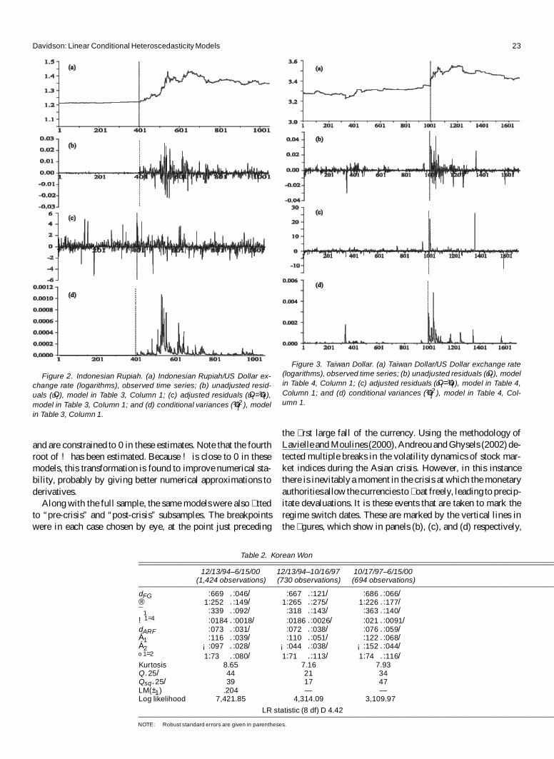
Figure 2. Indonesian Rupiah. (a) Indonesian Rupiah/US Dollar ex-change rate (logarithms), observed time series; (b) unadjusted resid-uals ( Out ), model in Table 3, Column 1; (c) adjusted residuals ( Out = O¾t ),model in Table 3, Column 1; and (d) conditional variances ( O¾ 2

t ), modelin Table 3, Column 1.

and are constrained to 0 in these estimates. Note that the fourthroot of ! has been estimated. Because ! is close to 0 in thesemodels, this transformation is found to improve numerical sta-bility, probably by giving better numerical approximations toderivatives.

Along with the full sample, the same models were also � ttedto “pre-crisis” and “post-crisis” subsamples. The breakpointswere in each case chosen by eye, at the point just preceding

Figure 3. Taiwan Dollar. (a) Taiwan Dollar/US Dollar exchange rate(logarithms), observed time series; (b) unadjusted residuals ( Out ), modelin Table 4, Column 1; (c) adjusted residuals ( Ou t= O¾t ), model in Table 4,Column 1; and (d) conditional variances ( O¾ 2

t ), model in Table 4, Col-umn 1.

the � rst large fall of the currency. Using the methodology ofLavielle and Moulines (2000), Andreou and Ghysels (2002) de-tected multiple breaks in the volatility dynamics of stock mar-ket indices during the Asian crisis. However, in this instancethere is inevitably a moment in the crisis at which the monetaryauthoritiesallow the currencies to � oat freely, leading to precip-itate devaluations. It is these events that are taken to mark theregime switch dates. These are marked by the vertical lines inthe � gures, which show in panels (b), (c), and (d) respectively,

Table 2. Korean Won

12/13/94–6/15/00 12/13/94–10/16/97 10/17/97–6/15/00(1,424 observations) (730 observations) (694 observations)

dFG :669 .:046/ :667 .:121/ :686 .:066/® 1:252 .:149/ 1:265 .:275/ 1:226 .:177/¯1 :339 .:092/ :318 .:143/ :363 .:140/

!1=4 :0184 .:0018/ :0186 .:0026/ :021 .:0091/dARF :073 .:031/ :072 .:038/ :076 .:059/Á1 :116 .:039/ :110 .:051/ :122 .:068/Á2 ¡:097 .:028/ ¡:044 .:038/ ¡:152 .:044/

º1=2 1:73 .:080/ 1:71 .:113/ 1:74 .:116/Kurtosis 8.65 7.16 7.93Q.25/ 44 21 34Qsq.25/ 39 17 47LM(±1) .204 — —Log likelihood 7,421.85 4,314.09 3,109.97

LR statistic (8 df) D 4.42

NOTE: Robust standard errors are given in parentheses.

24 Journal of Business & Economic Statistics, January 2004

Table 3. Indonesian Rupiah

1/01/96–12/31/99 1/01/96–7/11/97 7/14/97–12/31/99(1,045 observations) (400 observations) (645 observations)

dFG :496 .:042/ :588 .:104/ :54 .:054/® 2:94 .:85/ 1:81 .1:49/ 2:92 .1:59/

!1=4 :0099 .:0015/ :011 .:002/ :037 .:007/Á1 :047 .:032/ ¡:038 .:055/ :097 .:041/

º1=2 1:52 .:038/ 1:54 .:120/ 1:51 .:071/Kurtosis 14.6 2.4 1.1Q.25/ 37 22 29Qsq.25/ 27 19 22LM(dARF ) .012 — —LM(±1) 2.31 — —Log likelihood 5,889.68 2,978.46 2,917.85

LR statistic (5 df) D 12.18

NOTE: Robust standard errors are given in parentheses.

the estimated series Out, Out= O¾t , and O¾ 2t from the HYGARCH

model in each case.An examination of these results leads to three conclusions.

First, the three structures estimated are not wholly dissimilar,but each has distinctive features. In particular, the Won exhibitsquite a complex structure of autocorrelation,although this maybe due to the fact that the higher leptokurtosis of the other twoshock series has the effect of masking any autocorrelation thatmay be present. Second, however, they more closely resembleeach other than the currencies analyzed in Table 1. The mostnoteworthy feature is, of course, the large values of the ® para-meter in each case, especially for the Rupiah and Taiwan dollar.

Third, and perhaps most remarkable, is the stability of thesemodels across the pre-crisis and post-crisis regimes. In all threecases the large ® value is common to both periods, and the otherparameters are also generally close. The last line of each tableshows the likelihood ratio statistic for the test of model stabil-ity across the sample. Note that this cannot be interpreted as anasymptotic chi-squared test, because the breakpoints have beenchosen with reference to the data—that is, the most extremecontrast has been drawn in each case. Therefore, the correct nulldistribution of this statistic is the distribution of the maximumlog-likelihood ratio over all breakpoints. These critical valuesmust exceed the nominal chi-squared values. The statistic forthe Won is actually within the nominal acceptance region forthe 5% test, and that for the Rupiah is only slightly outside it.Overall, these results provide little evidence for changes in the

model following the crisis, and the residual plots in panels (c)of Figures 1–3 (from the model � tted to the full sample) pro-vide another view of this evidence. In two out of three cases, atleast, it would appear impossible to detect the breakpoint withcon� dence “by eye.”

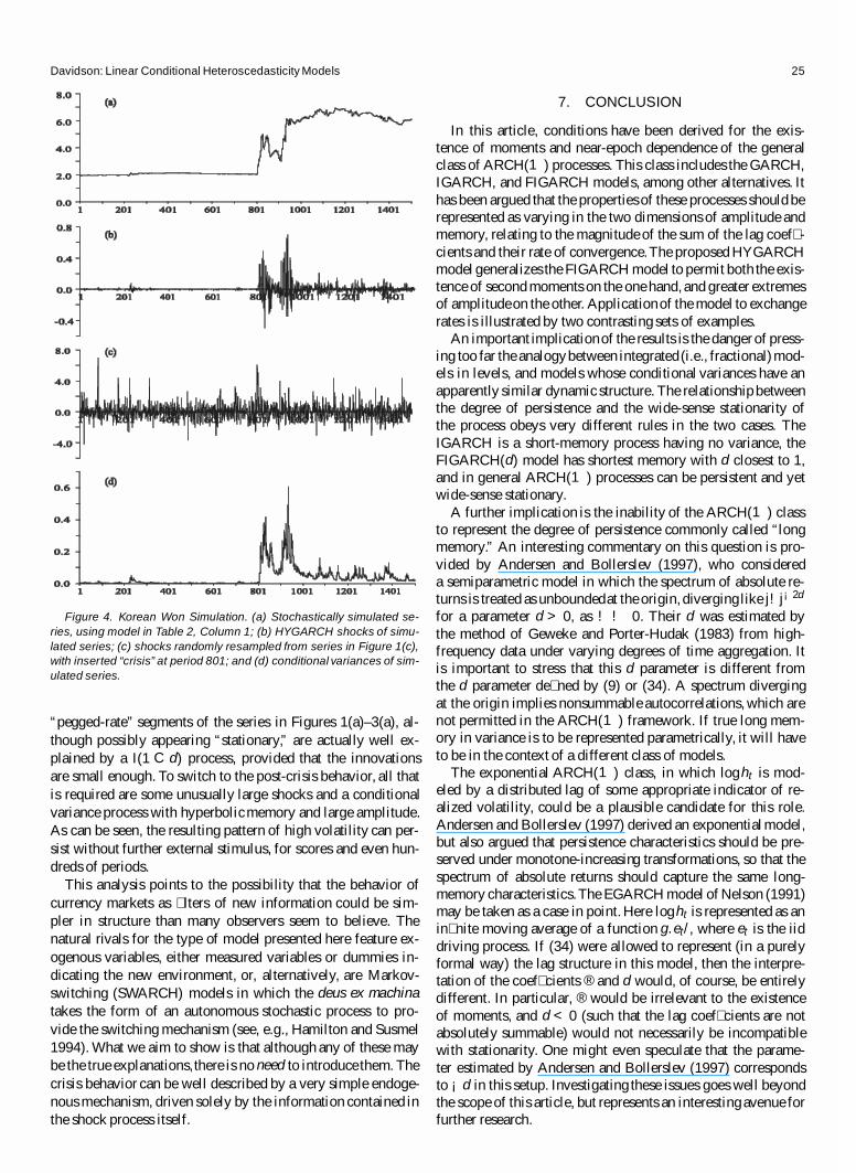
One further piece of evidence on the performance of thesemodels is presented in Figure 4. This is a simulation usingthe model of the Korean Won, driven by shocks randomly re-sampled from the residuals of the same model, as shown inFigure 4(c). The data shown were generated after letting theprocess run for 2,000 presample periods, to remove dependenceon initial conditions.A “crisis” was introducedby inserting intothe (otherwise randomly drawn) sequence a succession of � vepositive shocks, beginning at period 801. The values arbitrar-ily chosen were 4.2, 6.0, 3.3, 2, and 5.1, expressed in standarddeviations, because that of the shock distribution is 1 by con-struction. Such a realization would be a fairly rare event underrandom resampling, although major exchange crises are simi-larly rare, so this is not inappropriate.

There is, of course, no suggestion that the model (essen-tially, a heteroscedastic random walk) always generates runsof this appearance. Several repetitions of the experiment wererequired to produce the case illustrated, selected for its resem-blance to the observed data. The point to be made here is merelythat the observed data, taken as a whole, are compatible withthis type of data-generation process. Speci� cally, the pre-crisis

Table 4. Taiwan Dollar

01/03/94–6/15/00 01/03/94–10/15/97 10/16/97–6/15/00(1,683 observations) (988 observations) (695 observations)

dFG :860 .:079/ 1:001 .:010/ :667 .:073/® 2:96 .:466/ 2:956 .:466/ 2:946 .:877/±1 :242 .:138/ :009 .:187/ :568 .:221/¯1 :635 .:043/ :606 .:042/ :726 .:136/

!1=4 :021 .:006/ :022 .:006/ :000037 .:004/Á1 ¡:075 .:024/ ¡:131 .:031/ ¡:007 .:037/

º1=2 1:47 .:010/ 1:46 .:010/ 1:46 .:019/Kurtosis 336 21 184Q.25/ 9.40 49 5.27Qsq.25/ .21 23 .11LM(dARF ) .037 — —Log likelihood 8,631.47 5,263.64 3,38.61

LR statistic (7 df) D 25.56

NOTE: Robust standard errors are given in parentheses.

Davidson: Linear Conditional Heteroscedasticity Models 25

Figure 4. Korean Won Simulation. (a) Stochastically simulated se-ries, using model in Table 2, Column 1; (b) HYGARCH shocks of simu-lated series; (c) shocks randomly resampled from series in Figure 1(c),with inserted “crisis” at period 801; and (d) conditional variances of sim-ulated series.

“pegged-rate” segments of the series in Figures 1(a)–3(a), al-though possibly appearing “stationary,” are actually well ex-plained by a I(1 C d) process, provided that the innovationsare small enough. To switch to the post-crisis behavior, all thatis required are some unusually large shocks and a conditionalvariance process with hyperbolicmemory and large amplitude.As can be seen, the resulting pattern of high volatility can per-sist without further external stimulus, for scores and even hun-dreds of periods.

This analysis points to the possibility that the behavior ofcurrency markets as � lters of new information could be sim-pler in structure than many observers seem to believe. Thenatural rivals for the type of model presented here feature ex-ogenous variables, either measured variables or dummies in-dicating the new environment, or, alternatively, are Markov-switching (SWARCH) models in which the deus ex machinatakes the form of an autonomous stochastic process to pro-vide the switching mechanism (see, e.g., Hamilton and Susmel1994). What we aim to show is that although any of these maybe the true explanations,there is no need to introduce them. Thecrisis behavior can be well described by a very simple endoge-nous mechanism, driven solely by the information contained inthe shock process itself.

7. CONCLUSION

In this article, conditions have been derived for the exis-tence of moments and near-epoch dependence of the generalclass of ARCH(1) processes. This class includes the GARCH,IGARCH, and FIGARCH models, among other alternatives. Ithas been argued that the properties of these processes should berepresented as varying in the two dimensions of amplitude andmemory, relating to the magnitude of the sum of the lag coef� -cients and their rate of convergence.The proposed HYGARCHmodel generalizes the FIGARCH model to permit both the exis-tence of second moments on the one hand, and greater extremesof amplitudeon the other. Applicationof the model to exchangerates is illustrated by two contrasting sets of examples.

An important implicationof the results is the dangerof press-ing too far the analogybetween integrated (i.e., fractional)mod-els in levels, and models whose conditional variances have anapparently similar dynamic structure. The relationship betweenthe degree of persistence and the wide-sense stationarity ofthe process obeys very different rules in the two cases. TheIGARCH is a short-memory process having no variance, theFIGARCH(d) model has shortest memory with d closest to 1,and in general ARCH(1) processes can be persistent and yetwide-sense stationary.

A further implication is the inability of the ARCH(1) classto represent the degree of persistence commonly called “longmemory.” An interesting commentary on this question is pro-vided by Andersen and Bollerslev (1997), who considereda semiparametric model in which the spectrum of absolute re-turns is treated as unboundedat the origin, diverging like j!j¡2d

for a parameter d > 0, as ! ! 0. Their d was estimated bythe method of Geweke and Porter-Hudak (1983) from high-frequency data under varying degrees of time aggregation. Itis important to stress that this d parameter is different fromthe d parameter de� ned by (9) or (34). A spectrum divergingat the origin implies nonsummable autocorrelations, which arenot permitted in the ARCH(1) framework. If true long mem-ory in variance is to be represented parametrically, it will haveto be in the context of a different class of models.

The exponential ARCH(1) class, in which loght is mod-eled by a distributed lag of some appropriate indicator of re-alized volatility, could be a plausible candidate for this role.Andersen and Bollerslev (1997) derived an exponential model,but also argued that persistence characteristics should be pre-served under monotone-increasing transformations, so that thespectrum of absolute returns should capture the same long-memory characteristics.The EGARCH model of Nelson (1991)may be taken as a case in point. Here loght is represented as anin� nite moving average of a function g.et/, where et is the iiddriving process. If (34) were allowed to represent (in a purelyformal way) the lag structure in this model, then the interpre-tation of the coef� cients ® and d would, of course, be entirelydifferent. In particular, ® would be irrelevant to the existenceof moments, and d < 0 (such that the lag coef� cients are notabsolutely summable) would not necessarily be incompatiblewith stationarity. One might even speculate that the parame-ter estimated by Andersen and Bollerslev (1997) correspondsto ¡d in this setup. Investigating these issues goes well beyondthe scope of this article, but represents an interesting avenue forfurther research.

26 Journal of Business & Economic Statistics, January 2004

ACKNOWLEDGMENTS

This research was supported by the ESRC under awardL138251025.The author is most grateful to an anonymous ref-eree for suggestions for simplifying the proofs for Section 3,and also to Soyeon Lee for providinguseful comments and alsothe Asian crisis datasets used in Section 6.2.

APPENDIX: PROOFS OF THEOREMS

A.1 Proof of Theorem 1

Because ¾ 2t ¸ ! and EtCm

t¡m¾ 2t ¸ !, the inequality

kut ¡ EtCmt¡mutkp · !¡1=2k¾ 2

t ¡ EtCmt¡m¾ 2

t kp

follows by a minor extension of lemma 4.1 of Davidson (2002),replacing 2 with p ¸ 1. Therefore, in view of stationarity, it suf-� ces to prove the inequalities

k¾ 2t ¡ EtCm

t¡m¾ 2t kp · Cpm¡± (A.1)

for Cp > 0, for p D 1 and p D 2. Repeated substitution leads to,for given m, the decomposition

¾ 2t D ! C

1X

jD1

µje2t¡j¾

2t¡j

D !

³1 C

1X

j1D1

µj1e2t¡j1

C1X

j1D1

1X

j2D1

µj1µj2e2t¡j1

e2t¡j1¡j2

C ¢ ¢ ¢

C1X

j1D1

¢ ¢ ¢1X

jmD1

µj1 ¢ ¢ ¢ µjm e2t¡j1 ¢ ¢ ¢ e2

t¡j1¡¢¢¢¡jm

´

C1X

j1D1

¢ ¢ ¢1X

jmC1D1

µj1 ¢ ¢ ¢ µjmC1

£ e2t¡j1

¢ ¢ ¢ e2t¡j1¡¢¢¢¡jmC1

¾ 2t¡j1¡¢¢¢¡jmC1

:

(A.2)

To prove part (a), � rst note that

E­­e2

t¡j1¢ ¢ ¢ e2

t¡j1¡¢¢¢¡jp ¡ E¡e2

t¡j1¢ ¢ ¢e2

t¡j1¡¢¢¢¡jp

­­F tCmt¡m

¢­­»

D 0 j1 C ¢ ¢ ¢ C jp · m

· 2 otherwise,

using the Jensen inequality and law of iterated expectations inthe second case. Similarly,

E­­e2

t¡j1¢ ¢ ¢ e2

t¡j1¡¢¢¢¡jmC1¾ 2

t¡j1¡¢¢¢¡jmC1

¡ E¡e2

t¡j1¢ ¢ ¢ e2

t¡j1¡¢¢¢¡jmC1¾ 2

t¡j1¡¢¢¢¡jmC1jF tCm

t¡m

¢­­· 2M2;

where M2 is de� ned after (15). Next, de� ne

Tp D1X

j1D1

¢ ¢ ¢1X

jpD1

f j1C¢¢¢Cjp>mg. j1; : : : ; jp/µj1 ¢ ¢ ¢ µjp

·

Á 1X

jDm=pC1

µj

!

Sp¡1

· C

Á 1X

jDm=pC1

j¡1¡±

!Sp¡1

D O.p±m¡±Sp¡1/;

where the � rst inequality uses the fact that maxf j1; : : : ; jpg >

m=p when j1 C ¢ ¢ ¢ C jp > m. Because S < 1, applying the trian-gle inequality yields

E­­¾ 2

t ¡ EtCmt¡m¾ 2

t

­­· 2!

mX

pD1

Tp C 2M2SmC1

D O

Á

m¡±mX

pD1

p±Sp¡1

!

D O.m¡±/:

To prove part (b), note similarly that®®e2

t¡j1¢ ¢ ¢ e2

t¡j1¡¢¢¢¡jp ¡ E¡e2

t¡j1¢ ¢ ¢ e2

t¡j1¡¢¢¢¡jp

­­F tCmt¡m

¢®®2

(D 0 j1 C ¢ ¢ ¢ C jp · m

· 2¹p=24 otherwise,

whereas®®e2

t¡j1 ¢ ¢ ¢ e2t¡j1¡¢¢¢¡jmC1

¾ 2t¡j1¡¢¢¢¡jmC1

¡ E¡e2

t¡j1 ¢ ¢ ¢ e2t¡j1¡¢¢¢¡jmC1

¾ 2t¡j1¡¢¢¢¡jmC1

­­F tCmt¡m

¢®®2

· 2¹.mC1/=24 M1=2

4 :

Therefore, Minkowski’s inequality gives

®®¾ 2t ¡ EtCm

t¡m¾ 2t

®®2 · 2!

mX

pD1

Tp¹p=24 C 2¹

.mC1/=24 M1=2

4 SmC1

D O

Á

m¡±mX

pD1

p±.¹1=24 S/p¡1

!

D O.m¡±/:

A.2 Proof of Theorem 2

The proof of Theorem 1 is modi� ed as follows. For part (a),note that because ½ > 1 and S < 1, there exists " > 0 such that

QS D1X

jD1

µ 1¡"j < 1: (A.3)

There is no loss of generality in setting 1 < C < ½ . In this case,de� ning Q½ D ½" > 1 and QC D C", note that 1 < QC < Q½. Thennote that

Tp D1X

j1D1

¢ ¢ ¢1X

jpD1

f j1C¢¢¢Cjp>mg. j1; : : : ; jp/µj1 ¢ ¢ ¢ µjp

D1X

j1D1

¢ ¢ ¢1X

jpD1

f j1C¢¢¢Cjp>mg. j1; : : : ; jp/

£ jµj1 ¢ ¢ ¢ µjp j"jµj1 ¢ ¢ ¢ µjp j

1¡"

Davidson: Linear Conditional Heteroscedasticity Models 27

· QCp Q½¡m QSp

D QCp¡m QSp. QC Q½¡1/m: (A.4)

Therefore,

E­­¾ 2

t ¡ EtCmt¡m¾ 2

t

­­· 2!

mX

pD1

Tp C 2M2­­µj1 ¢ ¢ ¢ µjmC1

­­" QSmC1

D O¡m max

© QC¡m; QSmª. QC Q½¡1/mg

¢: (A.5)

To prove part (b), choose " > 0 such that QS DP1

jD1 µ 1¡"j <

¹."¡1/=24 . On the assumptions, C can be chosen without loss of

generality such that 1 < ¹"=24

QC < Q½ . Therefore,®®¾ 2

t ¡ EtCmt¡m¾ 2

t

®®2

· 2!

mX

pD1

Tp¹p=24 C 2¹

.mC1/=24 M1=2

4 jµj1 ¢ ¢ ¢ µjmC1 j" QSmC1

D O¡m max

©¡¹

"=24

QC¢¡m

;¡QS¹

.1¡"/=24

¢mª¡¹

"=24

QC Q½¡1¢m¢:

A.3 Proof of Theorem 3

Let

hmt D !

Á

1 CmX

j1D1

µj1e2t¡j1 C

mX

j1D1

m¡j1X

j2D1

µj1µj2e2t¡j1e

2t¡j1¡j2 C ¢ ¢ ¢

CmX

j1D1

¢ ¢ ¢m¡j1¡¢¢¢¡jm¡1X

jmD1

µj1 ¢ ¢ ¢ µjm e2t¡j1

¢ ¢ ¢ e2t¡j1¡¢¢¢¡jm

!

:

Then, using (A.2),

¾ 2t ¡ hm

t

D !

Á 1X

j1DmC1

µj1e2t¡j1 C

C1X

j1D1

1X

j2D1

f j1Cj2>mg. j1; j2/µj1µj2e2t¡j1

e2t¡j1¡j2

C ¢ ¢ ¢

C1X

j1D1

¢ ¢ ¢1X

jmD1

f j1C¢¢¢Cjm>mg. j1; : : : ; jm/µj1 ¢ ¢ ¢ µjm

e2t¡j1

¢ ¢ ¢ e2t¡j1¡¢¢¢¡jm

!

C1X

j1D1

¢ ¢ ¢1X

jmC1D1

µj1 ¢ ¢ ¢ µjmC1

£ e2t¡j1 ¢ ¢ ¢ e2

t¡j1¡¢¢¢¡jmC1¾ 2

t¡j1¡¢¢¢¡jmC1

D !.U1 C ¢ ¢ ¢ C Um/ C Vm;

where the last equality de� nes U1; : : : ;Um and Vm. The depen-dence of these terms on t is implicit but not indicated for easeof notation. By subadditivity,

P.j¾ 2t ¡hm

t j > ±/ · P.!jU1 C¢ ¢ ¢CUmj > ±=2/CP.Vm > ±=2/;

and the approach is to bound each term separately. First, notethat EjUpj D Tp, as de� ned in (A.4). Under the assumptions,

Tp · Cp½¡m1X

j1D1

¢ ¢ ¢1X

jpD1

f j1C¢¢¢Cjm>mg. j1; : : : ; jm/½m¡j1¡¢¢¢¡jp

D O.Sp½¡m/; (A.6)

and note that S · C=.½ ¡ 1/: Therefore, by subadditivity andthe Markov inequality,

P

Á

!

mX

pD1

jUpj > ±=2

!

· P

Ám[

pD1

»Up >

±!

2m

¼ !

·mX

pD1

P

³Up >

±!

2m

´

· 2m

±!

mX

pD1

Tp D O

³m2

³C

½.½ ¡ 1/

´m´:

Next, consider Vm. Let

QS D1X

jD1

µ 1C"j ; (A.7)

where " > 0 is to be chosen. [Note that although(A.7) is similarto the expression in (A.3), here the sign on " is reversed, and inthis case the sum may exceed 1.] By subadditivity,note that

P.Vm > ±=2/

· P

Á 1[

j1D1

¢ ¢ ¢1[

jmC1D1

©QSmC1­­µj1 ¢ ¢ ¢ µjmC1

­­¡"

£ e2t¡j1

¢ ¢ ¢ e2t¡j1¡¢¢¢¡jmC1

¾ 2t¡j1¡¢¢¢¡jmC1

> ±=2ª!

·1X

j1D1

¢ ¢ ¢1X

jmC1D1

P¡QSmC1

­­µj1 ¢ ¢ ¢ µjmC1

­­¡"

£ e2t¡j1

¢ ¢ ¢ e2t¡j1¡¢¢¢¡jmC1

¾ 2t¡j1¡¢¢¢¡jmC1

> ±=2¢:

(A.8)

Rewrite the probabilities in (A.8) in the form

P¡e2

t¡j1¢ ¢ ¢ e2

t¡j1¡¢¢¢¡jmC1> B. j1; : : : ; jmC1/

¢;

where

B. j1; : : : ; jmC1/ D±jµj1 ¢ ¢ ¢ µjmC1 j"

2QSmC1¾ 2t¡j1¡¢¢¢¡jmC1

:

For brevity, write

NP.¢/ D P¡¢­­Ft¡j1¡¢¢¢¡jmC1¡1

¢;

where Ft represents the sigma � eld generated by fes; s · tg, andhence ¾ 2

t¡j1¡¢¢¢¡jmC1may be held conditionally � xed under NP.

Consider the sequence

log¡e2

t¡j1 ¢ ¢ ¢ e2t¡j1¡¢¢¢¡jmC1

¢D

mX

pD1

log e2t¡j1¡¢¢¢¡jp

28 Journal of Business & Economic Statistics, January 2004

for m D 1; 2; : : : : Because the et are iid random variables, theCLT implies that for large m, the distribution of the sum isapproximately Gaussian with mean ¡m³ and variance m¿ 2,where ¿2 D var.loge2

t /. Note that by the Jensen inequality,

³ D ¡E.log e2j / > ¡ logE.e2

j / D 0:

Hence, for large enough m,

NP¡e2

t¡j1¢ ¢ ¢ e2

t¡j1¡¢¢¢¡jmC1> B. j1; : : : ; jmC1/

¢

D NP³

log.e2t¡j1

¢ ¢ ¢ e2t¡j1¡¢¢¢¡jmC1

/ C m³

¿p

m

>logB. j1; : : : ; jmC1/ C m³

¿p

m

´

Dexp

©¡ .log B. j1;:::; jmC1/Cm³/2

2¿ 2m

ªp

2¼.logB. j1; : : : ; jmC1/ C m³ /

£¡1 C O.logB. j1; : : : ; jmC1/ C m³ /¡2¢

: (A.9)

Here the second equality is obtained, assuming that

logB. j1; : : : ; jmC1/ C m³ > 0

(to be established below) from the asymptotic expansion of theGaussian probability function, (see 26.2.12 of Abramowitz andStegun 1965). Note that the error in the expansion is condition-ally of O.m¡2/.

Because flog¾ 2t g is a stationary sequence by assumption, and

hence Op.1/,

logB. j1; : : : ; jmC1/

m

D"

mlog

­­µj1 ¢ ¢ ¢ µjmC1

­­¡ log QS C Op.1=m/: (A.10)

As m increases, the conditional probability expression in (A.9)(suitably renormalized so that it does not vanish) is con-verging in probability to a nonstochastic limit, which neces-sarily matches that of the large-m unconditional probability.Henceforth, this formula is modi� ed by neglecting the termsof Op.1=m/. First, note that

0 · 1m

log­­µj1 ¢ ¢ ¢ µjmC1

­­· logµmax;

where µmax D maxj¸1 µj . The denominator in (A.9) is there-fore always positive if ³ > log QS, which henceforth is assumed.Next, note that

exp©¡

¡¡" log

­­µj1 ¢ ¢ ¢ µjmC1

­­¡ m log QS C m³¢2¢¯

2¿2mª

·­­µj1 ¢ ¢ ¢ µjmC1

­­"³=¿ 2

£ exp

»¡m

³." log µmax ¡ log QS/2 C 2³ log QS C ³ 2

2¿2

´¼:

(A.11)

Let LS be de� ned by

LSmC1 D1X

j1D1

¢ ¢ ¢1X

jmC1D1

­­µj1 ¢ ¢ ¢ µjmC1

­­"³=¿ 2

:

Combining (A.8)–(A.11) yields, for large enough m,

P.Vm > ±=2/

· LSmC1exp

©¡m

¡ ." log µmax¡log QS/2C2³ log QSC³ 2

2¿ 2

¢ªp

2¼m.³ ¡ log QS/

D O

³exp

»¡

m

2¿ 2

¡2³ log QS ¡ 2¿ 2 log LS

C ." logµ1 ¡ log QS/2 C ³ 2¢¼ ´

:

For the right side expression to vanish as m ! 1 requiresthat the sum of terms in parentheses in the exponentbe positive.Using ³ > log QS, the suf� cient condition,

3 log2 QS > 2¿2 log LS; (A.12)

is obtained.Consider the “worst case” in which µj D C½¡j . Sub-

stituting QS D C1C"=.½ 1C" ¡1/ and LS D C"³=¿ 2=.½ "³=¿ 2 ¡1/ into

(A.12) gives

3¡.1 C "/ logC ¡ log.½1C" ¡ 1/

¢2

> 2¿ 2¡"³ =¿ 2 logC ¡ log

¡½"³=¿ 2 ¡ 1

¢¢:

By taking " large enough, this can be made arbitrarily close to

3¡.1 C "/2.logC ¡ log½/

¢2> 2."³ logC ¡ "³ log½/

> 2".logC ¡ log½/2;

which holds for any choice of C and ½ . It follows that ³ > log QSis suf� cient, which proves part (b) of the theorem. In turn,C < ½ ensures that log QS · 0 for large enough " > 0, whichproves part (a).

[Received June 2001. Revised April 2003.]

REFERENCES

Abramowitz, M., and Stegun, I. A. (1965), Handbook of Mathematical Func-tions, New York: Dover Publications.

Andersen, T. G., and Bollerslev, T. (1997), “Heterogeneous Information Ar-rivals and Return Volatility Dynamics: Uncovering the Long Run in HighVolatility Returns,” Journal of Finance, 3, 975–1005.

Andreou, E., and Ghysels, E. (2002), “Detecting Multiple Breaks in Finan-cial Market Volatility Dynamics,” Journal of Applied Econometrics, 17,579–600.

Baillie, R. T., Bollerslev, T., and Mikkelsen, H. O. (1996), “Fractionally Inte-grated Generalized Autoregressive Conditional Heteroscedasticity,” Journalof Econometrics, 74, 3–30.

Baillie, R. T., Cecen, A. A., and Han, Y.-W. (2000), “High-FrequencyDeutsche mark–U.S. Dollar Returns: FIGARCH Representations and Non-Linearities,” Multinational Finance Journal, 4, 247–267.

Baillie, R. T., and Osterberg, W. P. (2000), “Deviations From Daily UncoveredInterest Rate Parity and the Role of Intervention,” Journal of InternationalFinancial Markets Institutions and Money, 10, 363–379.

Beltratti, A., and Morana, C. (1999), “Computing Value at Risk With High-Frequency Data,” Journal of Empirical Finance, 6, 431–455.

Bollerslev, T. (1986), “Generalized Autoregressive Conditional Heteroscedas-ticity,” Journal of Econometrics, 31, 307–327.

Box, G. E. P., and Pierce, D. A. (1970), “The Distribution of Residual Autocor-relations in Autoregressive-Integrated Moving Average Time Series Mod-els,” Journal of the American Statistical Association, 65, 1509–1526.

Brunetti, C., and Gilbert, C. L. (2000), “Bivariate FIGARCH and FractionalCointegration,” Journal of Empirical Finance, 7, 509–530.

Davidson: Linear Conditional Heteroscedasticity Models 29

Davidson, J. (1994), Stochastic Limit Theory—An Introduction for Econome-tricians, Oxford, U.K.: Oxford University Press.

(2002), “Establishing Conditions for the Functional Central Limit The-orem in Nonlinear and Semiparametric Time Series Processes,” Journal ofEconometrics, 106, 243–269.

(2003), “Time Series Modelling, Version 3.1,” available atwww.cf.ac.uk/carbs/econ/davidsonje/software.html.

De Jong, R. M. (1997), “Central Limit Theorems for Dependent HeterogeneousProcesses,” Econometric Theory, 13, 353–367.

Ding, Z., and Granger, C. W. J. (1996), “Modelling Volatility Persistenceof Speculative Returns: A New Approach,” Journal of Econometrics, 73,185–215.

Doornik, J. A. (1999), Object-Oriented Matrix Programming Using Ox(3rd ed.), London: Timberlake Consultants Press.

Engle, R. F. (1982), “Autoregressive Conditional Heteroscedasticity With Es-timates of the Variance of United Kingdom In� ation,” Econometrica, 50,987–1007.

Engle, R. F., and Bollerslev, T. (1986), “Modelling the Persistence of Condi-tional Variances,” Econometric Reviews, 5, 1–50.

Geweke, J., and Porter-Hudak, S. (1983), “The Estimation and Applicationof Long-Memory Time Series Models,” Journal of Time Series Analysis, 4,221–238.

Giraitis, L., Kokoszka, P., and Leipus, R. (2000), “Stationary ARCH Models:Dependence Structure and Central Limit Theorem,” Econometric Theory, 16,3–22.

Granger, C. W. J. (2002), “Long Memory, Volatility, Risk and Distribution,”working paper, University of California San Diego, Dept. of Economics.

Granger, C. W. J., and Teräsvirta, T. (1993), Modelling Nonlinear EconomicRelationships, Oxford, U.K.: Oxford University Press.

Hamilton, J. D., and Susmel, R. (1994), “Autoregressive Conditional Het-eroscedasticity and Changes in Regime,” Journal of Econometrics, 64,307–333.

He, C., and Teräsvirta, T. (1999), “Fourth-Moment Structure of theGARCH( p; q) Process,” Econometric Theory, 15, 824–846.

Karonasos, M. (1999), “The Second Moment and the Autocovariance Functionof the Squared Errors of the GARCH Model,” Journal of Econometrics, 90,63–76.

Kazakevi Ïcius, V., and Leipus, R. (2002), “On Stationarity in the ARCH(1)Model,” Econometric Theory, 18, 1–16.

Lavielle, M., and Moulines, E. (2000), “Least Squares Estimation of an Un-known Number of Shifts in Time Series,” Journal of Time Series Analysis,20, 33–60.

Lee, S.-W., and Hansen, B. E. (1994), “Asymptotic Theory for theGARCH(1;1) Quasi-Maximum Likelihood Estimator,” Econometric Theory,10, 29–52.

Li, W. K., and Mak, T. K. (1994), “On the Squared Residual Autocorrelationin Nonlinear Time Series With Conditional Heteroscedasticity,” Journal ofTime Series Analysis, 15, 627–636.

Lumsdaine, R. L. (1996), “Consistency and Asymptotic Normality of theQuasi-Maximum Likelihood Estimator in IGARCH(1;1) and CovarianceStationary GARCH(1;1) Models,” Econometrica, 64, 575–596.

McLeod, A. I., and Li, W. K. (1983), “Diagnostic Checking ARMA Time SeriesModels Using Squared-Residual Autocorrelations,” Journal of Time SeriesAnalysis, 4, 269–273.

Nelson, D. B. (1990), “Stationarity and Persistence in the “GARCH(1;1)Model,” Econometric Theory, 6, 318–334.

(1991), “Conditional Heteroscedasticity in Asset Returns: A New Ap-proach,” Econometrica, 59, 347–370.

Pötscher, B. M., and Prucha, I. R. (1991), “Basic Structure of the AsymptoticTheory in Dynamic Nonlinear Econometric Models, Part I: Consistency andApproximation Concepts,” Econometric Reviews, 10, 125–216.