Detecting The Expected Rate of Return Volatility of Financing Instruments of Indonesian Islamic...

Tazkia Islamic Finance and Business Review

Volume 9.1.

60

Detecting The Expected Rate of Return Volatility of

Financing Instruments of Indonesian Islamic Banking

through GARCH Modeling (Generalized Autoregressive

Conditional Heteroscedasticity)

Nurul Huda1, Amrin Barata, SST

2

1YARSI University, Jakarta, Indonesia [email protected] ;

2Badan Pusat Statistik RI (Statistics Indonesia), Jakarta, Indonesia [email protected]/ [email protected]

Abstract

Objective - Islamic banks are banks which its activities, both fund raising and funds distribution are on

the basis of Islamic principles, namely buying and selling and profit sharing. Islamic banking is aimed at

supporting the implementation of national development in order to improve justice, togetherness, and

equitable distribution of welfare. In pursuit of supporting the implementation of national development,

Islamic banking often faced stability problems of financing instruments being operated. In this case, it is

measured by the gap between the actual rate of return and the expected rate of return. The individual

actual RoR of this instrument will generate an expected rate of return. This raises the gap or difference

between the actual rate of return and the expected rate of return of individual instruments, which in this

case is called the abnormal rate of return. The stability of abnormal rate of return of individual

instruments is certainly influenced by the stability of the expected rate of return. Expected rate of return

has a volatility or fluctuation levels for each financing instrument. It is also a key element or material

basis for the establishment of a variance of individual instruments. Variance in this case indicates the

level of uncertainty of the rate of return. Individual variance is the origin of the instrument base for

variance in the portfolio finance that further a portfolio analysis. So, this paper is going to analyze the

level of expected RoR volatility as an initial step to see and predict the stability of the fluctuations in the

rate of return of Indonesian Islamic financing instruments.

Methods – Probability of Occurence, Expected Rate of Return (RoR) and GARCH (Generalized

Autoregressive Conditional Heteroscedasticity).

Results - The expected RoR volatility of the murabaha and istishna financing instruments tend to be more

volatile than expected RoR volatility of musharaka and qardh financing instruments.

Conclusions – The uncertainity of Musharaka and qardh financing instruments tend to be more stable

than other Islamic financing instruments.

Keywords : Islamic Financing Instruments, Expected rate of return, GARCH

mailto:[email protected]

mailto:[email protected]/


Volume 9.1.

61

Abstrak

Tujuan - Bank syariah ialah bank yang dalam aktivitasnya, baik penghimpunan dana maupun penyaluran dananya memberikan dan mengenakan imbalan atas dasar prinsip syariah yaitu jual beli dan bagi hasil. Perbankan Syariah bertujuan menunjang pelaksanaan pembagunan nasional dalam rangka meningkatkan keadilan, kebersamaan, dan pemerataan kesejahteraan rakyat. Dalam mencapai tujuan menunjang pelaksanaan pembangunan nasional, perbankan syari’ah sering dihadapkan pada masalah kestabilan instrumen pembiayaan yang dijalankannya, dalam hal ini diukur melalui kesenjangan antara tingkat pengembalian sebenarnya (actual rate of return) dengan tingkat pengembalian yang diharapkan (expected rate of return). Actual RoR individual instrumen ini nantinya akan menghasilkan suatu expected rate of return (tingkat pengembalian yang diharapkan). Hal ini menimbulkan adanya kesenjangan atau selisih antara actual rate of return dan expected rate of return individual instrumen, yang dalam hal ini disebut abnormal rate of return. Kestabilan Abnormalrate of return dari individual instrumen ini tentunya dipengaruhi oleh kestabilan expected rate of return. Expectedrate of return memiliki suatu volatilitas atau tingkat fluktuasi untuk setiap instrumen pembiayaan, serta merupakan unsur utama atau bahan dasar pembentukan suatu variance individual instrumen. Variance dalam hal ini menunjukan tinggi rendahnya ketidakpastian dari tingkat pengembalian tersebut. Dari variance individual instrumen inilah asal bahan dasar variance portofolio pembiayaan dalam suatu analisis portofolio yang lebih lanjut. Sehingga dari hal tersebutlah akan dilakukan suatu analisis terhadap tingkat volatilitas expected RoR sebagai langkah awal untuk melihat dan memprediksi kestabilan dari fluktuasi rate of return instrumen pembiayaan syariah Indonesia. Metode – Probability of Occurrence, Expected Rate of Return (R0R) dan GARCH (Generalized Autoregressive Conditional Heteroscedasticity). Hasil - Volatilitas expected RoR dari instrumen pembiayaan mudharabah,murabahah dan istishna cenderung lebih fluktuatif dibanding volatilitas expected RoR dari instrumen pembiayaan musyarakah dan qardh. Kesimpulan - Ketidakpastian instrumen pembiayaan musyarakah dan qardh cenderung lebih stabil dari instrumen pembiayaan syariah lainnya.

Kata kunci : Islamic Financing Instruments, Expected rate of return, GARCH


Volume 9.1.

62

1. Introduction

Islamic banking effort for diversifying the financing product to become portfolio of financing (a

combination of more than one financial instrument) is very important to improve the return or

refund of Islamic banks, so that the growth of Islamic banking in Indonesia may increase and

the share of Islamic banking assets will be no longer far below conventional banks. However, an

obstacle in the business establishment of this financing portfolio is the need to examine the

behavior of the return of each Islamic financing instruments, namely how the expectations of

return of each instrument before the instruments combined with other instruments (a

combination of two, three, four, or five financing instruments). Whether expected rate of return

of each form of financing shows a stable behavior or unstable behavior.

Financing return is not the only obstacle in this case, but also the risk which is a measure of the

uncertainty of the expected rate of return to be earned in the future of the financing portfolio.

Islamic banking will certainly avoid the high risk of finance in contracting the finance portfolio

to investors. It is also important to consider the level of fluctuations (volatility) of the gap

between the actual rate of return and the expected rate of return of Islamic financing

instruments, considering the monthly time series data in the financial sector or financial (rate of

return) very high level of volatility. This gap is called the abnormal rate of return. The high

volatility is characterized by a phase in which the fluctuation is relatively high and then

becomes and then returns to its high fluctuation. In other words, the data has no constant

average and variant. Thus, the volatility of the abnormal rate of return of Islamic financing

instruments is also a measure of uncertainty as additional consideration to establish the

financing portfolio in this study to look at the volatility of the expected rate of return as the

element. By this, the research problems raised in this research is how the fluctuation level of

expected rate of return volatility which is an element of uncertainty (variance) of the Islamic

bank financing instruments in Indonesia during the period of 2004 (March) until 2014 (April) ?

Engle (2001) in a paper entitled "The Use of ARCH / GARCH Models in Applied

Econometrics" said the GARCH model can be used as a technique to construct an equation that

measures the volatility (foresee or predict the variance) of the stock return and portfolio.

Alessandro (2007) in a paper entitled "An Out-of-sample Analysis of Mean-Variance Portfolios

with Orthogonal GARCH Factors" wrote that the GARCH model, both the mean and variance

models used to predict the return and risk over several periods ahead. Based on consideration of

forecasting the return and risk of the portfolio, it will be considered where the best portfolio.


Volume 9.1.

63

Research conducted by Savickas in the paper entitled "Event-Induced Volatility And Test For

Abnormal Performance" wrote that the GARCH model is the best model that can capture the

effect of volatility of stock return data, compared to other methods such as the method of mean

rank and standardized cross-sectional.

Research conducted by Otavio Alberto (2005) in peper titled "Brazilian Market Reaction to

Equity Issues Announcements" wrote that the GARCH method is better in estimating for return

of a stock than the OLS estimates.

2. Methodology

This study uses secondary data measured in time series. Islamic Banking in Indonesia in this

study is Islamic Commercial Bank (BUS) and Islamic Business Unit of a Conventional Bank

(UUS), Islamic Rural Bank (BPRS). Source data is taken from Bank Indonesia, that is Islamic

Banking Statistics (SPS) and on the website of Bank Indonesia (www.bi.go.id) and the

Financial Services Authority (OJK) published every month. Time period in this study is from

March 2004 until April 2014, using historical monthly data. The software used in this study is a

Microsoft Office Excel 2007 and Eviews 6.0.

This study consists of several variables, namely the equivalent rate of return variable of each

financing instruments of Islamic banking.

This study uses a quantitative approach. First of all, the events probability of each financing

instrument will be identified. Of the likelihood and the actual rate of return obtained here will be

expected rate of return of Islamic financing instruments. Then the econometric analysis will be

conducted to support the analysis of return and risk, in this case the analysis is to detect the

volatility of portfolio returns through modeling ARCH/GARCH (p, q).

The expected return of one and more than one financial instrument is defined as follows :

N

i

iii rpRE1

)(

(1)

Where ip is probability of occurrence of return, and ir is rate of return (RoR) instrument.

Because Islamic finance theory states that future profits should not be ascertained, then this


Volume 9.1.

64

calculation uses historical data as a predictor (good predictor-proxy) for the probability of

occurrence ( ip) above.

Econometric analysis using time series data in this case is to obtain the data seris portfolio

return volatility of financial instruments of Islamic banking in Indonesia, through modeling

ARCH / GARCH. The steps are described below.

2.1 Stationarity Test Data Through the Unit Root Test

The first step that must be done in the estimation of the economic model with time series data is

to test the stationarity in the data or also called a stationary stochastic process. Stationarity test

data can be performed by using the Phillips-Perron test at the same level (level or different) to

obtain a stationary data.

2.2 Box-Jenkis Method (ARIMA)

Box-Jenkins models is one of the techniques of data time series forecasting models based only

on the observed behavior of variable data. This model is technically known as a model

autoregressivi integrated moving average (ARIMA). The main reason for the use of this model

movements in economic variables studied such as the movement of exchange rates, stock prices,

returns, inflation is often difficult to explain by economic theories. The Box-Jenkins models

terdirir of several models: autoregressive (AR), moving average (MA), autoregressive-moving

average (ARMA) and autoregressive integrated moving average (ARIMA).

Autoregressive Model

AR model shows the predicted value of the dependent variable yt is only a linear function of the

number of actual yt earlier. For autoregressive models of order p, observation yt is formed from

the weighted average of past observations, p periods back and deviation of the current period.

For example, the value of the variable Yt is only influenced by the value of the variable or

inaction of the previous period, the first such models called autoregressive model of the first

level or abbreviated AR (1). AR model equation (1) can be written as follows:

ttt eyy 11 (2)

Where : y = dependent variable

yt-1 = first lag of y


Volume 9.1.

65

In general, the form of a general model of autoregressive (AR) can be expressed in the

following equation:

tptpttt eyyyy ...2211

(3)

Where: yt = dependent variable

yt-p = pth

lag of y

et = residual (error term)

p = level of AR

Residuals in equation (3) is as OLS model has the characteristics of an average value of zero,

constant variance and not interconnected. AR model thus shows that the predicted value of the

yt dependent variable is only a linear function of the number of actual yt previous.

Moving Average Model

Model MA stated that the predictive value of the dependent variable yt is only affected by the

residual value of the previous period. Model MA has a magnitude of the order which is denoted

by the letter 'q', so that the model is usually written by the MA (q). This model assumes that

each observation is formed from the weighted average deviation (disturbance) q periods

backwards. For example, if the value of the dependent variable yt is only affected by the

residual value of the previous period, the so-called first-level model of the Supreme Court or

abbreviated with MA (1). Model MA (1) can be written in the form of the following equation:

11 ttt eey

(4)

Where : et = residual

et-1 = first lag of residual.

In general, the form of the moving average (MA) model can be expressed in the form of the

following equation :

qtqttttt eeeeey ...332211

(5)

Where : 1 , 2 , ..., q = parameters which can be positive or negative.

In this case, it is assumed also that:


Volume 9.1.

66

);,0(~ 2

et Niide covariances

0,0 kk

Or 0),(;)()(;0)( 22 kttettt eeEeVareEeE

With these assumptions, the mean of the MA process is not dependent on the time that

is )( tyE

. Model MA is the dependent variable y prediction model based on a linear

combination of the previous residual whereas the AR model to predict the y variable is based on

the value of y the previous period.

Autoregressive-Moving Average Model

Sometimes stationary random process that can not be modeled by an AR (p) or MA (q) process

because has both characteristics. Therefore, this kind of process that needs to be approached

with a model mixture of autoregressive and moving average, known as ARMA model (p,q).

This model is expressed in the form:

qtqttptpttt eeeyyyy ...... 112211 (6)

Because the process is assumed to be constant over time, then the mean will be constant

over time (not bound by time).

For the ARMA (1,1), the model is as follows :

1111 tttt eeyy

(7)

2.3 Selecting ARIMA Model

The best ARIMA models selection using measurement that is used as goodness model

indicator for ARCH/GARCH models as follow:

a. Akaike’s Information Criterion (AIC) with the formula: n

k

n

RSS 2log

(8)

b. Schwarz Criterion (SC) with the formula: nn

k

n

RSSloglog

(9)

Where :


Volume 9.1.

67

RSS = residual sum of squares

k = number of independent variables

n = number of observation.

Selection of the best model selected by comparing the value of the AIC or SC values in the can,

the minimum value or the smallest is the best model. It also uses Adjusted R2 value of the

largest, with the following formula:

kn

nR

nTSS

knRSSR

1)1(1

)1/(

)/(1 22 (10)

Where : RSS = Residual sum of squares

TSS = Total sum of squares

The AIC criterion gives greater weight than 2R in the case of the addition of the independent

variables. According to this criterion, a good model if the smallest AIC value. While the criteria

for SC gives greater weight than AIC. SC that’s Low indicates a better model. There are several

advantages of AIC and SC criteria compared with 2R . First, both of these criteria can be used

for in-sample forecasting (whether in accordance with the existing data) as well as out-of-

sample forecasting (whether in accordance with the values that occur in the future). Second,

these criteria can also be used for nested model selection and non-nested models.

2.4 ARCH and GARCH Model

Time series data, especially the data in financial sector, has a high degree of volatility. Volatility

measures the average fluctuations of time series data, but it is developed further with the

emphasis on the value of variation (statistical variables that describe how far the changes and

fluctuations in the value distribution of the average value) of financial data. That is, the value of

volatility as the value of the variance of the fluctuations (return data).

The presence of high volatility is certainly difficult for researchers to make estimates and

predictions of the movement of these variables. High volatility shown by a phase in which the

fluctuation is relatively high and then followed a low fluctuation and high return. In other

words, the data is averaged and the variance is not constant. Sometimes a variant of error does

not depend on the independent variable, but these variants change with the change of time.

Application of financial data with the characteristics usually on modeling the return of capital

markets, inflation and interest rates. Thus volatility patterns indicate heteroscedasticity because

there are variants error whose magnitude depends on the volatility of the error in the past.


Volume 9.1.

68

Autoregressive Moving Average (ARMA) Model is often used in the modeling of time series

data. This model has a stationarity assumption on the data and constant residual variance

(homoscedasticity). This assumption is not easily fulfilled on time series data data financially.

The financial data has its own characteristics compared to the time series data in general, which

shows high volatility following the period of time that shows volatility, variance for a long

period of time the data is constant but there are some periods where the data variance is

relatively high. This is called conditionally heteroskedastic. If detected, the conditionally

heteroskedastic autoregressive moving average models (ARMA) no longer appropriate to use.

The data get heteroscedasticity properties like this can be modeled by Autoregresive

Conditional Heteroscedasticity (ARCH) which was introduced by Robert Engle.

ARCH method is a refinement of the ARMA method. At ARMA, the variance is not the center

of attention when one uses the model is that we want to see a large deviation in the forecast,

which means also the contribution of predictor variables that we input into the model works. For

that ARCH is required to see the pattern of residual variance, so that we can evaluate and

improve the return forecasts that we make, because this method further support the existence of

other predictor variables are unknown or are not included in the model. ARCH designed

specifically to produce models and forecasting (forecast) due to the presence of conditionals

variance. There are several reasons underlying the establishment of ARCH models and forecast

volatility:

1. The need to analyze the risks of the assets that we have or the value of an option.

2. forecasting confidence intervals are at different times, so to get the interval can be obtained

from the model variance of the error.

3. a more efficient estimator can be obtained if heteroskesdatisitas can be handled first.

To explain how ARCH models formed, suppose we have the following linear regression model:

ttt exbxbby 221110 (11)

)var(; 22

110

2

tttt ee (12)

Note that )var( te

described by two components:

1. constant component : 0

2. variable component : 2

11 te ; that is called ARCH com;ponent.


Volume 9.1.

69

On this model, te heteroscedasticity, conditional in 1te

. By adding information "conditional"

or "conditional" the estimator of ,, 10 bband 2b

become more efficient.

ARCH model above, where )var( te

depends only on the volatility of the last period, as in

2

110

2

tt e , that is called ARCH(1) model. While in general, when it

)var( te depends

on the volatility of the past few periods as 22

22

2

110

2 ... ptpttt eee is called

ARCH(p) model or written by :

p

i

itit e1

2

0

2

(13)

In this model, in order to be a positive variance ( )0)var( 2 e , then the restriction must be

made, namely : 00

dan 10 1

.

Note the number of ARCH (p) above. With a relatively large number of p will result in the

number of parameters to be estimated. The more parameters to be estimated can result in

reduced precision of the estimator. To overcome these problems, so that the estimated

parameters are not too much, the )var( te

can be used the following models :

2

11

2

110

2

ttt e

(14)

This model is called the GARCH (1,1) because 2

t depend on 2

1te and

2

1t each of which has

a time lag. Similarly, ARCH models, in order to be a positive variance

( )0)var( 2 e ,then on this model should also be made restrictions, namely : 10 ;0 and

;01 and

111 .

As ARCH model, the GARCH model can also be estimated by Maximum Likelihood technique.

In general the, )var( te

can be represented by the form :

22

11

22

110

2 ...... qtqtptptt ee or written by:

q

i

iti

p

i

itit e1

2

1

2

0

2

(15)

The Model above is called GARCH(p,q) model.


Volume 9.1.

70

The model shows that the amount of )var( te

is estimated depending on 2e and also depending

on 2 in the past.

At the time series data of finance of the ARCH/GARCH element or a form of authoregressive

of residual quadratic phase which is characterized by high fluctuations and then followed a low

fluctuation and high return.

2.5 Steps in Determining ARCH / GARCH Model

Steps in determining the ARCH / GARCH model are as follows:

1. Identify the mean models

Determine the model parameters model of flats which have a significant predictor. Modeling of

the average necessary to produce residual to be estimated changes, so this averaging models has

an important role in modeling volatility. Volatility is highly dependent on the type of model

averaging formed. Averaging can use regression models or ARMA, in this study the mean

model using ARMA model.

2. Testing the conditional variance heterogeneity

The employed tests to detect the presence of the ARCH / GARCH is lagrange multiplier test

(LM) or a pattern of squares residuals via correlogram, not using the Durbin-Watson test. This

is because the Durbin-Watson test has some disadvantages. First, this test is only valid if the

independent variable is random or stochastic. If this test to enter the independent variables that

are non-stochastic like inserting variable inaction (lag) of the dependent variable as the

independent variable called autoregressive models, the Durbin-Watson test can not be used.

Second, the Durbin-Watson test is only valid if the relationship between the residual

autocorrelation in the first-order or first-order autoregressive abbreviated AR (1). This test can

not be performed for higher autoregressive models such as AR (2), AR (3), and so on. Third,

this model can not be used in case a moving average (moving average) of residual higher order.

Based on the above weaknesses, the Breusch and Godfrey develop autocorrelation test is more

commonly known as Lagrange Multiplier test (LM). To understand the LM test, it will be made

the following simple regression model :

tt eXY 110 (16)


Volume 9.1.

71

We make assumption that residual models follow autoregressive models of order p or

abbreviated AR (p) as follows :

tptpttt veeee ...2211

(17)

Where vt in this model have the characteristic that is ;)var(;0)( 2 tt vvE

and

0),cov( 1 tt vv.

So the null hypothesis of no autocorrelation in the model AR (p) can be formulated as follows :

0...:

0...:

211

210

p

p

H

H

If we accept H0 then say no autocorrelation in the model. If the sample is large, then according

Breusch and Godfrey, the model in equation (17) will follow the distribution of Chi-Squares df

p is the17length of inaction as residuals in equation (2). Statistically calculated value of Chi-

Squares can be calculated using the following formula :

22)( pRpn

(18)

If 2)( Rpn which is a chi-squares ( ) calculated is more than critical value chi-squares ( )

at a certain degree of confidence ( ), we reject the null hypothesis (H0). This means least, there

is a statistically significantly different from zero. It shows that there is a problem of

autocorrelation in the model, and vice versa. The determination of whether there is a problem of

autocorrelation can also be seen from the value of the probability chi-squares ( ) . If the

probability value is greater than the selected value then we accept H0 which means do not exist

autocorrelation, and vice versa.

In short, the LM test is used to detect the presence of ARCH processes, namely the residual

variance heterogeneity influenced squared residual previous period or so-called residual

variance heterogeneity conditional (conditional heteroscedasticity) in the time series.

Hypotheses for LM test can also be formulated as follows :

H0: ARCH error does not exist (indicated by the value of F statistic with the probability > )

H1: ARCH error exists (indicated by the value of F statitic with the probability < )


Volume 9.1.

72

Beside LM heteroscedasticty test, it also could be seen from residual and squared residuals

through correlogram. If there is no autocorrelation on the residual but on the squared residual,

it’s mean that there is heteroscedasticity. Hypotheses that’s used on the testing through

correlogram as follows.

H0: there is no autocorrelation (indicated value of Q Statistically ACF and PACF of the

probability > )

H1: there is autocorrelation (indicated value Q of the ACF and PACF Statistically the

probability < )

3. Estimation of the parameters of ARCH / GARCH model

Determination of the alleged parameters by using the maximum likelihood method (maxsimum

likelihood). If the residual is not normal then allegedly parameters with Maxsimum Quasi-

likelihood method. Maximum likelihood, in the estimation process requires equality in the

distribution of error is Normal ),0( 2 . While in some cases, errors sometimes do not follow

the model of the Normal distribution ),0( 2 . Typically the data transformation to normality

assumption is fulfilled in order inference estimator done right. However, to obtain the

appropriate transformer often have difficulty. Therefore, the quasi-maximum likelihood method

(QMLE) offered to resolve the error assumption is violated.

QMLE help reinforce the results of the maximum likelihood inference if an error assumption is

violated. QMLE method is a method of estimation variance-covariance performed on the model

parameters assuming the error is violated. Based on the variance-covariance value formed a new

inference drawn up to determine the significance of the model parameter estimator. QMLE still

utilizing the maximum likelihood method as a basis, so that the calculation of the variance-

covariance quasi also the values resulting from the maximum likelihood method.

GARCH (p, q) process assumes that (Zt) is i.i.d. random variable, namely Zt~N(0,1) so the

likelihood function can be used. Assuming that the likelihood function is Gaussian, then the log-

likelihood function is as follows:

T

t

tT lT

L1

)(2

1)(

where .)(

)(ln)(2

2

2

t

t

ttl

(19)


Volume 9.1.

73

Gaussian likelihood function does not require, in other words, the process (Zt) does not need to

be Gaussian white noise, LT-called quasi-likelihood function. In the use of quasi maximum

likelihood (QML), the way to suppress the choice of heteroscedasticity consistent covariance

(Bollerslev-Wooldridge) on the choice of model ARCH / GARCH in eviews 6.0. By using this

option, the parameters which allegedly remained consistent and asymptotically still valid.

4. diagnosis models

Examination of the model is done by checking whether there are heteroscedasticty, using

ARCH-LM test or correlogram case of the conditional variance heterogeneity test phase above.

Ljung Box test is used to test the feasibility of the model. The model is feasible if the remnant

had not had a pattern (random) or in other words having no autocorrelation lag between a

remnant for all k.

5. Selection of the best model

If at this stage of the model diagnostics are some models that fit the selected best model. Criteria

for the best model is to have a good size and the goodness of the model coefficients are real.

Size used as an indicator of goodness models to models ARCH / GARCH as follows :

a. Akaike’s Information Criterion (AIC) with the formula: n

k

n

RSS 2log

(20)

b. Schwarz Criterion (SC) with the formula:

nn

k

n

RSSloglog

(21)

where :

RSS = residual sum of squares

k = number of independent variables

n = number of observation.

Selection of the best model selected by comparing the value of the AIC or SC values in the can,

the minimum value or the smallest dalah best model. Because the ARCH model estimation

using the maximum likelihood method is not based on the evaluation of the regression line

Adjusted R2 but based on the log likelihood. Model selection criteria so that also uses the log

likelihood great value.


Volume 9.1.

74

3. Results and Discussion

3.1 Volatility of Expected Rate of Return (RoR)

Stationarity Test

In this study, expected rate of return variable of each financing instrument has been

tested for its stationarity.

Table 1 Summary of the unit root test with constant use at the level of [I(0)]

Expected rate of

return

Phillips-Perron test statistic

Prob.*

(1) (2) (3)

Istishna* -3.7355 0.0047

Mudharabah* -3.5885 0.0073

Musyarakah* -4.5806 0.0003

Murabahah* -5.3750 0.0000

Qardh* -5.6485 0.0000

Source: output eviews 6

* significant at α = 5%

Based on Table 1, the initial level [I (0)] of the Phillips-Perron test showed that on the whole

there is no unit root variables, so the data is stationary, it is shown that the value of prob* or p-

value less than α = 5 % (accept Ho) that is not contained unit root. By this, that variable

expected rate of return volatility of istishna, mudaraba, murabaha, musharaka and qardh

financing instruments calculation to be performed.

Volatility Calculation of Expected Rate of Return Financing Instruments

Volatility measures the average fluctuations of time series data, but it is developed further with

the emphasis on the value of variation (statistical variables that describe how far the changes

and fluctuations in the value distribution of the average value) of financial data. That is, the

value of volatility as the value of the variance of the fluctuations (return data).

Calculations are performed with the ARCH/GARCH model volatility. In this study, modeling

ARCH/GARCH is performed on expected rate of return variables that have high volatility

characteristics. Expected rate of return is the value of the rate of return (RoR) which is expected.

Changes in the expected rate of return in this study is not only seen for its value, but also its

volatility or the speed of the rise and fall expected rate of return also observed. In determining


Volume 9.1.

75

the ARCH/GARCH model consists of two stages: determine the mean models and variance

models.

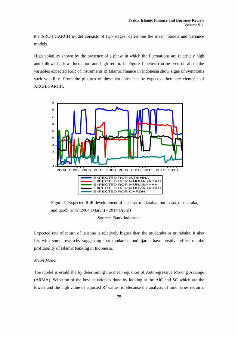
High volatility shown by the presence of a phase in which the fluctuations are relatively high

and followed a low fluctuation and high return. In Figure 1 below can be seen on all of the

variables expected RoR of instruments of Islamic finance in Indonesia show signs of symptoms

such volatility. From the pictures of these variables can be expected there are elements of

ARCH/GARCH.

Figure 1 Expected RoR development of istishna, mudaraba, murabaha, musharaka,

and qardh (in%) 2004 (March) - 2014 (April)

Source: Bank Indonesia

Expected rate of return of istishna is relatively higher than the mudaraba or murabaha. It also

fits with some researchs suggesting that mudaraba and ijarah have positive effect on the

profitability of Islamic banking in Indonesia.

Mean Model

The model is establishe by determining the mean equation of Autoregressive Moving Average

(ARMA). Selection of the best equation is done by looking at the AIC and SC which are the

lowest and the high value of adjusted R2 values is. Because the analysis of time series requires

0

1

2

3

4

5

6

7

8

9

2004 2005 2006 2007 2008 2009 2010 2011 2012 2013

EXPECTED ROR ISTISHNA

EXPECTED ROR MUDHARABAH

EXPECTED ROR MURABAHAH

EXPECTED ROR MUSYARAKAH

EXPECTED ROR QARDH


Volume 9.1.

76

that the data should be stationary then the ARMA processing using the data at the level expected

RoR. The result of trial and error (trial and error) which has smallest value of AIC and SC and

the highest value of Adjusted R2i is summarized in the following table.

Table 2 Selection of the best ARMA models (mean models) of expected RoR variable

of financing instruments

Expected rate of

return

ARMA

AIC

SC

Adj R2

(1) (2) (3) (4) (5)

Istishna ARMA(1,1) 3.3742 3.4435 0.7113

MA(1) 4.0362 4.0822 0.4597

MA(2) 4.3809 4.3878 0.5729

Mudharabah AR(1) 2.7196 2.7658 0.6715

ARMA(2,1) 2.7056 2.7986 0.6752

MA(1) 3.2591 3.3051 0.4461

MA(2) 3.0414 3.1104 0.5580

Murabahah AR(1) 2.9547 3.0009 0.4043

MA(1) 3.1646 3.210 0.2596

MA(2) 3.0573 3.1263 0.3403

Musyarakah AR(1) 2.2354 2.2816 0.5659

AR(2) 2.1993 2,2690 0.5856

MA(1) 2.6006 2.6465 0.4075

MA(2) 2.4870 2.5559 0.4754

Qardh AR(1) 0.4209 0.4671 0.3778

AR(2) 0.3497 0.4193 0.4102

ARMA(2,2) 0.2098 0.3259 0,4954

Source : Bank Indonesia

Detection ARCH-error

After a mean models are formed, made an error in the detection of the presence of ARCH

models. In this study, the detection of the presence or absence of ARCH-error is using the

ARCH-LM test. ARCH-LM test results for ARMA equation of expected RoR financing

instruments for the equation shows that the expected variable ARMA RoR murabaha,

Musharaka and qardh statistics show obs * R-squared with smaller probability than α = 5%,

while the expected variable RoR istishna and mudaraba statistics show obs * R-squared with

smaller probability than α = 10%. Thus the hypothesis Ho is rejected, which states that there are

elements of ARCH. Because of the mean models kelimat above variables, the resulting error

contains elements that can be formed ARCH variance models.


Volume 9.1.

77

Variance Model

As in the process of establishing the model mean, variance formation step models also through a

process of trial and error. However, after testing the normality of the residual model of ARCH /

GARCH that will be selected. Test results showed that all models of ARCH / GARCH has not

normally distributed residuals. It is marked with a p-value or probability of the Jarque-Bera that

less than 5% significance level, so that H0 is rejected, stating that the residuals do not follow a

normal distribution. To overcome this, the corrected standard errors in the subsequent

estimation using the Bollerslev-Wooldridge correction (Bollerslev-Wooldridge robust standard

errors and covariance) of the estimated quasi-maximum likelihood (QML). This is because

although the residual abnormal, resulting estimation of maximum quasi-likelihood estimation

(QML) remained consistent. So that the results of the estimated parameters remain valid even if

not asymptotically normally distributed. Then proceed to test the significance of parameters.

The final step in the determination of the variance of the model is to look at the value of the

smallest AIC and SC, as well as the largest log likelihood.

Table 3 Selection of the Best ARCH/GARCH Model (Variance Model) of Expected

RoR variable of Financing Instruments

Expected rate of

return

(1)

ARCH/GARCH

(2)

AIC

(3)

SC

(4)

Log-

likelihood

(5) Istishna GARCH(1,0) 3.3472 3.4627 -197.5

GARCH(1,2) 3.1758 3.33759 -185.14

GARCH(2,1) 3.3191 3.4808 -193.807

GARCH(2,2) 3.1958 3.3806 -185.347

Mudharabah GARCH(1,0) 2.7145 2.8307 -157.87

GARCH(1,1) 2.7297 2.8691 -157.78

GARCH(1,2) 2.7300 2.8927 -156.804

Murabahah GARCH(1,0) 2.7742 2.8666 -163.8385

GARCH(1,1) 2.5743 2.6898 -150.747

GARCH(0,1) 2.9534 3.0458 -174.683

Expected rate of

return

(1)

ARCH/GARCH

(2)

AIC

(3)

SC

(4)

Log-

likelihood

(5)


Volume 9.1.

78

Musyarakah GARCH(1,0) 2.1130 2.2292 -121.78

GARCH(1,2) 2.0441 2.2067 -115.645

GARCH(0,2) 2.0253 2.1646 -115.52

Qardh GARCH(1,0) -0.4170 -0.2544 32.0214

GARCH(2,2) -0.6288 -0.3966 47.734

GARCH(0,2) 0.1596 0.3454 -1.5771

Source: Bank Indonesia

In order to obtain the equation of ARCH / GARCH as follows:

To variance model of expected rate of return variables of istishna:

ht = 1,294 + 0,531 e2

t-1 + 0,231 σ2

t-1– 0,298 σ2

t-2 (22)

To variance model of expected rate of return variables of istishna mudharabah:

ht = 0,448 + 1,090 e2

t-1 (23)

To variance model of expected rate of return variables of istishna murabahah:

ht = 0,570 + 1,363 e2

t-1 + 0,317 σ2

t-1 (24)

To variance model of expected rate of return variables of istishna musyarakah:

ht = 0,0511 + 1,928 σ2

t-1 - 1,0142 σ2

t-2 (25)

To variance model of expected rate of return variables of istishna qardh:

ht = 0,0004 + 1,596 e2

t-1 + 1,1346 e2

t-2 – 0,391 σ2

t-1 + 0,149 σ2

t-2 (26)

Where : ht = σ2

t = variance of squared residuals at t-month

e2

t-p = squared residuals in (t-p)-month

σ2t-q = variance of squared residuals in (t-q)-month

Checking ARCH / GARCH Model

Terms for good model is that the ARCH element does not exist in the residual of variance

models and there is no autocorrelation in the error ARCH/GARCH models equation. ARCH-

LM test results for ARCH/GARCH equation for expected RoR variable financing instruments

for the equation shows that the GARCH (p, q) of expected RoR istishna, mudaraba, murabaha,

musharaka, and qardh variables show statistics obs* R-squared with probability more greater

than α = 5%. Thus the hypothesis Ho failed rejected stating there is no element of ARCH or no

heteroskedasticity on the model.


Volume 9.1.

79

Testing can be done by using the autocorrelation correlogram, or a unit root test. Test results

showed that all the statistics Q (Q-Stat) of expected RoR istishna and qardh financing

instruments variable is not statistically significant, with probability (prob) over α = 5%. This

means that the error does not contain the autocorrelation. For expected RoR mudaraba,

murabaha, and musharaka financing instruments variable, there is still a significant Q statistics

on some initial lag. However, after testing the unit root test stationarity, were error models are

stationary at level I (0) (statistically significant at α = 5%). Therefore concluded that the error of

the model does not contain the autocorrelation.

3.2 Overview Volatility of Expected Rate of Return Financing Selected

Volatility of expected rate of return is a risk of instability or uncertainty of the expected rate of

return financing instruments. ARCH/GARCH model volatility variable is used to form the

expected rate of return based on the best model. To obtain the volatility of expected rate of

return, first create the best ARIMA modeling each financing instrument as noted previously.

Furthermore, the detection of whether the residual variance of the data expected RoR is not

constant and varies from one period to another, or contain elements of heteroscedasticity. To

detect this using ARCH-LM test. However, the residual variance not only depend on the

residual period, but also depends on the residual variance ago period. So perform the modeling

generalized autoregressive conditional heteroscedasticity (GARCH) as in the previous stage.

From this is derived volatility GARCH of expected rate of return.

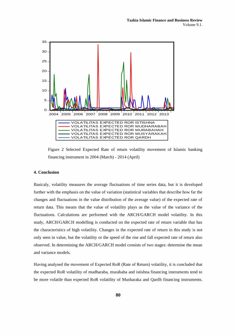
The movement of the volatility expected RoR can be seen in Figure 2 below. From this figure it

is concluded that the expected RoR volatility of the financing instrument of mudharaba,

murabaha, istishna tend to be more volatile than the expected RoR volatility of Musharaka and

qardh financing instruments. This means that the expected RoR volatility of the musharaka and

qardh financing instruments tend to be more stable than other instruments.


Volume 9.1.

80

Figure 2 Selected Expected Rate of return volatility movement of Islamic banking

financing instrument in 2004 (March) - 2014 (April)

4. Conclusion

Basicaly, volatility measures the average fluctuations of time series data, but it is developed

further with the emphasis on the value of variation (statistical variables that describe how far the

changes and fluctuations in the value distribution of the average value) of the expected rate of

return data. This means that the value of volatility plays as the value of the variance of the

fluctuations. Calculations are performed with the ARCH/GARCH model volatility. In this

study, ARCH/GARCH modelling is conducted on the expected rate of return variable that has

the characteristics of high volatility. Changes in the expected rate of return in this study is not

only seen in value, but the volatility or the speed of the rise and fall expected rate of return also

observed. In determining the ARCH/GARCH model consists of two stages: determine the mean

and variance models.

Having analysed the movement of Expected RoR (Rate of Return) volatility, it is concluded that

the expected RoR volatility of mudharaba, murabaha and istishna financing instruments tend to

be more volatile than expected RoR volatility of Musharaka and Qardh financing instruments.

0

5

10

15

20

25

30

35

2004 2005 2006 2007 2008 2009 2010 2011 2012 2013

VOLATILITAS EXPECTED ROR ISTISHNA

VOLATILITAS EXPECTED ROR MUDHARABAH

VOLATILITAS EXPECTED ROR MURABAHAH

VOLATILITAS EXPECTED ROR MUSYARAKAH

VOLATILITAS EXPECTED ROR QARDH


Volume 9.1.

81

This means that abnormal RoR volatility of Musharaka and Qardh financing instruments tend

to be more stable than other Islamic financing instruments.

Regardless of the factors that influence the volatility of the Islamic financing instruments, this

result gives an idea of how stable the five Islamic financing instruments to be developed as well

as anticipated in developing Islamic banking in Indonesia, whether it will be used for the basic

preparation of diversification product or financing portfolio serve as an opportunity to invest.

References

Alamsyah, Halim. (2012). Perkembangan dan Prospek Perbankan Syariah Indonesia:

Tantangan Dalam Menyongsong MEA 2015. Paper Milad ke-8 Ikatan Ahli Ekonomi

Islam (IAEI) di Ruang Auditorium Lt. 2 Gd. Badan Kebijakan Fiskal Kementerian

Keuangan Republika Indonesia. Jakarta

Bank Indonesia. (2004-2015). Statistik Perbankan Syariah Indonesia. Jakarta: BI

Barata, Amrin. (2013). Penentuan Komposisi Optimal Kontrak Instrumen Pembiayaan

Perbankan Syariah di Indonesia melalui Pembentukan Efficient Portfolio Frontier tahun

2004-2012 (Pendekatan Risk-Return dan Pemodelan GARCH. Jakarta : Sekolah Tinggi

Ilmu Statistok (STIS).

Bilbiee, Florin. (2000). Applications of ARCH Modelling in Financial Time Series: the Case of

Germany. Coventry, West Midlands CV4 7AL, United Kingdom : Department of

Economics University of Warwick.

Cardinali, Alessandro. (2007). An Out-of-sample Analysis of Mean-Variance Portfolios with

Orthogonal GARCH Factors. International Econometric Review (IER) Volume 4, Issue

1, pages 1-16.

Edi,et all. (2009). Quasi-Maximum Likelihood untuk Regresi Panel Spasial [Paper]. Surabaya:

Institut Teknologi Sepuluh November (ITS).

Engle, Robert. (2001). The Use of ARCH/GARCH Models in Applied Econometrics. Jurnal of

Economic Perspectives. Volume 15, Number 4, Pages 157-168.

Huda, Nurul, and Nasution, Mustafa. (2009). Current Issues Lembaga Keuangan Syariah.

Jakarta: Kencana Prenada Media Group.

Ismal, Rifki. (2010). The Indonesian Islamic Banking (Theory and Practices). Bogor: Phd

Gramata Publishing.

Joko, Kandung. (2007). Pengaruh Volatilitas Nilai Tukar Dan Nilai Neto Ekspor Terhadap

Volatilitas Cadangan Devisa Indonesia Periode 1980-2006 [Skripsi]. Jakarta: Sekolah

Tinggi Ilmu Statistik (STIS).

Markowitx H.M. (1991). Foundations of Portfolio Theory. Journal of Finance. Volume 46,

Issue 2, pages 469–477.


Volume 9.1.

82

Muhamad. (2001). Teknik Perhitungan Bagi Hasil di Bank Syariah. Yogyakarta: UII Press.

Nachrowi, dan Usman, Hardius. (2006). Ekonometrika untuk Analisis Ekonomi dan Keuangan.

Jakarta: Lembaga Penerbit Fakultas Ekonomi Universitas Indonesia.

Obaidullah, Mohammed. (2005). Islamic Financial Services. Saudi Arabia: Islamic Economic

Research Center, University Jeddah.

Ribeiro, Otavio, and Shigueru, Alberto. (2005). Brazilian Market Reaction to Equity Issue

Announcements. Revista de Administração Contemporânea. Volume 9, No.spe2, Pages

36-46.

Lewis, Mervyn and Al-Qaoud, Latifa. (2001). Perbankan Syari’ah: Prinsip, Praktik, Prospek.

Jakarta : Serambi.

Lee, Sang and Hansen, Bruce. (1994). Asymptotic Theory For The Garch (1,1) Quasi-

Maximum Likelihoode Stimator. Econometric Theory, 10, 1994, 29-52.

Otoritas Jasa Keuangan. (2014). Statistik Perbankan Syariah Indonesia. Jakarta: OJK

Posedel, Petra. (2005). Properties and Estimation of GARCH(1,1) Model. Metodoloˇski zvezki,

Vol. 2, No. 2, 2005, 243-257.

Savickas, Robert. (2003). Event-Induced Volatility And Test For Abnormal Performance. The

Journal of Financial Research• Vol. XXVI, No. 2, Pages 165-178.

Supranto, Johanes. (2004). Statistik Pasar Modal Keuangan dan Perbankan. Jakarta: Rineka

Cipta.

Syafi’i, Muhammad4. (2001). Bank Syari’ah dari Teori ke Praktik. Jakarta: Gema Insani Press.

Widarjono, Agus. (2009). Ekonometrika Pengantar dan Aplikasinya. Yogyakarta: Ekonisia.

Yahya, Arya. (2011). Pengaruh Perilaku Kurs(Rp/US$) Terhadap Ekspor Nonmigas Dan

Produk Domestik Bruto Nonmigas Indonesia Periode 1993-2010 [Skripsi]. Jakarta:

Sekolah Tinggi Ilmu Statistik.

Yulianti, Rahmani. (2009). Manajemen Risiko Perbankan Syariah. Jurnal Ekonomi Islam Vol.

III, No. 2, P.151-165.

http://www.scielo.br/scielo.php?script=sci_serial&pid=1415-6555&lng=en&nrm=iso

Detecting The Expected Rate of Return Volatility of Financing Instruments of Indonesian Islamic...

Documents

Transcript of Detecting The Expected Rate of Return Volatility of Financing Instruments of Indonesian Islamic...