An Empirical Comparison of Realized Volatility, GARCH and ...
24
Estimation of Monthly Volatility: An Empirical Comparison of Realized Volatility, GARCH and ACD-ICV Methods Shouwei Liu School of Economics, Singapore Management University Yiu-Kuen Tse School of Economics, Singapore Management University February 2012 Abstract: We apply the ACD-ICV method proposed by Tse and Yang (2011) for the estimation of intraday volatility to estimate monthly volatility, and empirically compare this method against the re- alized volatility (RV) and generalized autoregressive conditional heteroskedasticity (GARCH) methods. Our Monte Carlo results show that the ACD-ICV method performs well against the other two meth- ods. Evidence on the Chicago Board Options Exchange volatility index (VIX) shows that it predicts the ACD-ICV volatility estimates better than it predicts the RV estimates. While the RV method is popular for the estimation of monthly volatility, its performance is inferior to the GARCH method. JEL Codes: C410, G120 Keywords: Autoregressive conditional duration, generalized autoregressive conditional heteroskedas- ticity, market microstructure, realized volatility, transaction data Acknowledgment: The authors gratefully acknowledge research support from the Center for Financial Econometrics of the Sim Kee Boon Institute for Financial Economics, Singapore Management University. Corresponding Author: Yiu-Kuen Tse, School of Economics, Singapore Management University, 90 Stamford Road, Singapore 178903, email: [email protected].
-
Upload
khangminh22 -
Category
Documents
-
view
1 -
download
0
Transcript of An Empirical Comparison of Realized Volatility, GARCH and ...

Estimation of Monthly Volatility: An Empirical Comparison ofRealized Volatility, GARCH and ACD-ICV Methods
Shouwei LiuSchool of Economics, Singapore Management University
Yiu-Kuen TseSchool of Economics, Singapore Management University
February 2012
Abstract: We apply the ACD-ICV method proposed by Tse and Yang (2011) for the estimation ofintraday volatility to estimate monthly volatility, and empirically compare this method against the re-alized volatility (RV) and generalized autoregressive conditional heteroskedasticity (GARCH) methods.Our Monte Carlo results show that the ACD-ICV method performs well against the other two meth-ods. Evidence on the Chicago Board Options Exchange volatility index (VIX) shows that it predictsthe ACD-ICV volatility estimates better than it predicts the RV estimates. While the RV method ispopular for the estimation of monthly volatility, its performance is inferior to the GARCH method.
JEL Codes: C410, G120
Keywords: Autoregressive conditional duration, generalized autoregressive conditional heteroskedas-ticity, market microstructure, realized volatility, transaction data
Acknowledgment: The authors gratefully acknowledge research support from the Center for FinancialEconometrics of the Sim Kee Boon Institute for Financial Economics, Singapore Management University.
Corresponding Author: Yiu-Kuen Tse, School of Economics, Singapore Management University, 90Stamford Road, Singapore 178903, email: [email protected].

1 Introduction
Many studies in the empirical finance literature on the risk-return relationship involve the estimation
of the monthly return volatility of stocks. Higher frequency (such as daily) data are usually not used
because returns are typically rather noisy, rendering the risk-return relationship in high frequency
difficult to establish. Furthermore, many studies examine the effects of macroeconomic variables on
asset pricing, and these variables are only available monthly or quarterly. For example, Schwert (1989)
constructed vector autoregression models involving monthly data of short-term interest rates, long-term
yields of high-quality and medium-quality bonds, inflation rates and industrial production to analyze
the dynamic structure of stock volatility. For some recent studies requiring estimates of monthly stock
volatility, see Goyal and Santa-Clara (2003), Bali, Cakici, Yan and Zhang (2005), Guo and Savickas
(2008), Ludvigson and Ng (2007), Jiang and Tian (2010) and Zhang (2010).
Since the seminal work of French, Schwert and Stambaugh (1987) and Schwert (1989), researchers
often use the sum of the squared daily stock returns over a month (or some modifications of it) as an
estimate of the monthly volatility of the stock. Later, Andersen, Bollerslev, Diebold and Ebens (2001)
and Andersen, Bollerslev, Diebold and Labys (2001) proposed to use the sum of the squared returns
of tick data to estimate intraday volatility, and called this estimate the realized volatility (RV). Since
then the literature on RV has expanded very quickly.
The estimation of intraday volatility using RV methods typically requires sampling over 5-min
intervals or shorter, with sampling over 1- or 2-min intervals not uncommon. Given the asymptotic
theories established in the litertaure and the availability of large numbers of return observations over
short durations in a trading day, the RV methods have a firm theoretical underpinning as a tool for
estimating intraday volatility. In contrast, in applying the RV methods to estimate monthly volatility
using daily data there are only approximately 21 return observations to compute each monthly estimate.
Thus, estimation errors may be a concern and may weaken the validity of the statistical inference. As
high-frequency data have become increasingly available we extend the use of monthly RV estimation to
these data.
2

Another line of research applies the autoregressive conditional heteroskedasticity (ARCH) model
of Engle (1982) and the generalized ARCH (GARCH) model of Bollerslev (1986) to estimate monthly
volatility. French, Schwert and Stambaugh (1987) estimated monthly volatility using a GARCH-in-mean
model, while Fu (2009) estimated monthly idiosyncratic risk using the exponential GARCH (EGARCH)
model of Nelson (1991). Monthly volatility can be estimated using GARCH type of models on monthly
data, or using these models on daily data from which aggregates of daily conditional variances form a
monthly estimate.
Recently, Tse and Yang (2011) proposed a method to estimate high-frequency volatility using the
autoregressive conditional duration (ACD) model of Engle and Russell (1998), called the ACD-ICV
method. They estimate high-frequency volatility (over a day or shorter intervals) by integrating the
instantaneous conditional return variance per unit time obtained from the ACD models. Unlike the RV
methods, which sample data over regular intervals, the ACD-ICV method samples price events based on
high-frequency transaction price changes exceeding a threshold. ACD models for the durations between
sequential price events are estimated using the quasi maximum likelihood method, and the conditional
variance over a given intraday interval is computed by integrating the instantaneous conditional variance
within the interval. The Monte Carlo results of Tse and Yang (2011) show that the ACD-ICV method
gives lower root mean-squared error than the RV methods in estimating intraday volatility. While Tse
and Yang (2011) focused on the estimation of intraday volatility, in this paper we apply the ACD-ICV
method to estimate monthly volatility.
The literature so far has little to say about the choice of the estimation method for monthly volatility.
While the RV approach seems to dominate the literature, the use of the GARCH type of models is not
uncommon. In addition, the ACD-ICV method may be a useful alternative, as it has been shown to
perform well for the estimation of intraday volatility. In this paper we compare the performance of the
RV, GARCH and ACD-ICV methods using Monte Carlo (MC) experiments and empirical data from
the New York Stock Exchange (NYSE). Our MC results show that the ACD-ICV method outperforms
the RV method in giving lower root mean-squared error. Indeed, it turns out that the GARCH method
performs better than the RV method in the MC experiments. We also examine the use of the Chicago
3

Board Options Exchange (CBOE) volatility index (VIX) as a predictor of the volatility for the next 30
days estimated by the ACD-ICV, RV and GARCH methods using the S&P500 index. Our results show
that VIX predicts the 30-day ACD-ICV volatility estimates better than it predicts the RV estimates.
The rest of the paper proceeds as follows. Section 2 summarizes the monthly volatility estimates
considered in this paper. In Section 3 we report some MC results on the comparison of the RV, GARCH
and ACD-ICV methods. The MC study suggests that the best results for the ACD-ICV method appear
to be obtained when the range of the return for defining the price event is about 0.15% to 0.35%. It
also shows that the ACD-ICV method performs very well against the RV method. Section 4 reports our
results for the estimation of monthly volatility using some empirical data from the NYSE. In Section 5
we examine the use of VIX as a predictor of the market volatility over the next 30 days, with market
volatility estimated using the ACD-ICV, RV and GARCH methods. Finally, Section 6 concludes.
2 Methods of Estimating Monthly Volatility
Volatility estimation over monthly or quarterly intervals dated back to the 1970s. Researchers in earlier
work adopted the 12-month rolling standard-deviation estimate as the volatility estimate of the centered
month, as in Officer (1973), Fama (1976), and Merton (1980). Schwert (1989) employed a two-step
rolling regression to construct monthly volatility, which allows the conditional mean return to vary over
time and allows different weights for the lagged absolute unexpected returns. Since the work of French,
Schwert and Stambaugh (1987), Schwert (1989), Schwert (1990a), Schwert (1990b) and Schwert and
Seguin (1990), the use of the sum of the squared daily returns over a month, called the RV method, has
emerged as the most popular method for the estimation of monthly stock volatility. On the other hand,
monthly volatility can also be estimated using GARCH models estimated with monthly data, or by
aggregating daily conditional variances over a month estimated from GARCH models with daily data.
In this section we summarize the methods of estimating monthly volatility examined in this study.
2.1 RV Method
Let ri denote the return on day i of the month, r̄ denote the average daily return of the month and N
denote the number of trading days in the month. The basic RV estimate of the variance of the month,
4

denoted by VD, is defined as
VD =N∑
i=1
(ri − r̄)2, (1)
which has been widely adopted in the literature.1 However, as this estimator uses only about 21
observations its accuracy may be a concern. As high-frequency data have become easily available, we
consider the use of transaction data to estimate monthly RV. For the purpose of using as much data as
possible, shorter sampling intervals are preferred. However, returns over short sampling intervals may
be contaminated by market microstructure noise. To balance between these two conflicting goals, we
use 5-min price data to calculate the RV and denote it by VR.2
2.2 GARCH Method
Another popular method for constructing monthly volatility is to use the GARCH model and its exten-
sions. In this paper, we adopt the EGARCH(1, 1) model defined by
log σ2t = ω + α
εt−1
σt−1+ β
∣∣∣∣ εt−1
σt−1
∣∣∣∣ + γ log σ2t−1, (2)
where εt is the residual of the return and σ2t is the conditional variance. We assume that the standardized
residual zt = εt/σt follows the generalized error distribution (GED) with density function
fZ(z) =ν exp
[−1
2
∣∣∣ zλ
∣∣∣ν]λ 21+ 1
ν Γ(
1ν
) , −∞ < z <∞, 0 < ν ≤ ∞, (3)
where ν > 0, Γ(·) denotes the gamma function and λ ≡ [2(−2/ν)Γ(1/ν)/Γ(3/ν)]1/2. We estimate the
EGARCH(1, 1) model using daily data and compute the daily conditional variance σ̂2t , for t = 1, · · · , N ,
over N days of the month. We then aggregate the estimated daily conditional variances and denote it
by VG, so that3
VG =N∑
t=1
σ̂2t . (4)
1French, Schwert and Stambaugh (1987) proposed a method to correct for the serial correlation in the return series.However, we find this method to be inferior to VD and we will not report its results in this paper.
2This is in contrast to Jiang and Tian (2005) and Becker, Clements and White (2007), who used 30-min data to computethe RV. To extend the use of equation (1) to intraday returns, we have to consider the treatment of overnight price jumps.We tried using the first price and the 5th-min price of the day to compute the overnight return. As the results are similarwe report only the case of using the first price. In VR only the return (not deviation from mean return) is used.
3In the MC study we also consider estimating the GARCH model using monthly data, with the monthly volatilityestimates directly computed without aggregation. The results, however, are poor and will not be reported.
5
2.3 ACD-ICV Method
The ACD model was first proposed by Engle and Russell (1998) to analyze the durations of transaction
data. Tse and Yang (2011) proposed to estimate intraday volatility by integrating the instantaneous
conditional variance per unit time estimated from the ACD model, resulting in the ACD-ICV method.
In this section, we first review the ACD-ICV method proposed by Tse and Yang (2011), followed by an
outline of the modification of this method for the estimation of monthly volatility.
Let t0, t1, · · · , tN denote a sequence of times for which ti is the time of occurrence of the ith price
event, which is said to have occurred if the cumulative change in the logarithmic transaction price
since the last price event is at least of a preset amount δ (whether upwards or downwards), called
the price range. Thus, xi = ti − ti−1, for i = 1, 2, · · · , N , are the intervals between consecutive price
events, called the price durations. Let Φi be the information set upon the transaction at time ti,
and denote ψi = E(xi |Φi−1), which is the conditional expectation of the transaction duration. If the
standardized durations εi = xi/ψi are independently and identically distributed as exponential variables,
the integrated conditional variance in the interval (t0, tN ), denoted by ICV, is given by
ICV = δ2N−1∑i=0
ti+1 − tiψi+1
. (5)
The implementation of the ACD-ICV method to estimate monthly volatility depends on the price
data available. In this paper we use higher-frequency transaction data. We ignore the overnight close of
the market and treat the first trade of each day as continuously away from the last trade of the previous
trading day. Given the return range δ we compile t1, · · · , tN−1 based on the continuous transaction
data as the price-event times over a month.
The use of equation (5) requires estimates of the conditional expected duration ψi+1. Following Tse
and Yang (2011) we adopt the augmented ACD (AACD) model (see Fernandes and Grammig (2006))
defined by
ψλi = ω + αψλ
i−1[|εi−1 − b|+ c(εi−1 − b)]υ + βψλi−1. (6)
We estimate the AACD model using the quasi maximum likelihood estimation (QMLE) method, with
the standardized duration assumed to be exponentially distributed. The ACD-ICV estimate of monthly
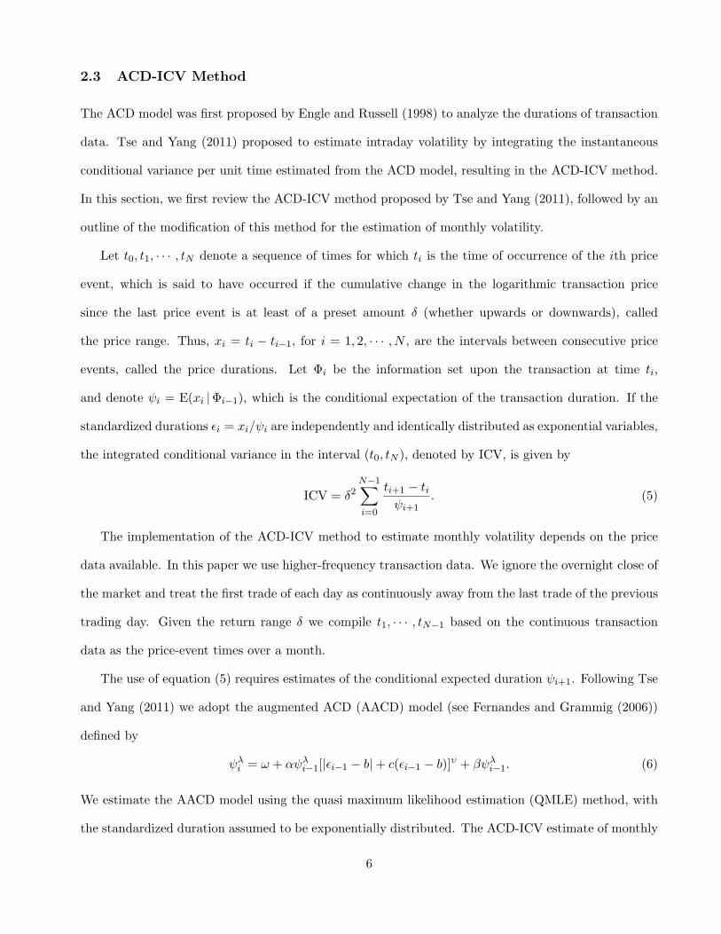
6
volatility, denoted by VA is computed as
VA = δ2N−1∑i=0
ti+1 − ti
ψ̂i+1
, (7)
where ψ̂i+1 is the QMLE of ψi+1. The choice of δ affects the fit of the ACD(1, 1) model for price duration,
and hence the performance of VA as an estimate of the monthly ICV. In our empirical application we
vary δ from 0.15% through 0.35% in steps of 0.05%, and denote the resulting estimates by VAj for
j = 1, · · · , 5, respectively, to correspond to δ being 0.15%, 0.20%, 0.25%, 0.30% and 0.35%.
3 Monte Carlo Study
We adopt the usual assumption in the empirical literature that the logarithmic stock price follows a
Brownian semimartingale (BSM). Denoting the stock price at time t by p(t) and defining p̃(t) = log p(t),
we assume
p̃(t) =∫ t
0µ(t) dt+
∫ t
0σ(t) dW (t), (8)
where µ(t) is the instantaneous drift rate, σ2(t) is the instantaneous variance and W (t) is a standard
Brownian process. For each MC sample, we generate data over 5 years, with a total of 60 months of
observations.
For the drift term µ(t) we consider two different artificial processes, which are plotted in Figure 1.
For the variance process σ2(t) we consider two methods: deterministic volatility and stochastic volatility
models, which will be described in the next two subsections. Given the drift term µ(t) and the variance
term σ2(t), we generate the logarithmic price series p̃(t) by the equation
p̃(t+ ∆t) = p̃(t) + µ(t) ∆t+ σ(t)√
∆t ε, (9)
where ε ∼ N(0, 1). We take ∆t to be one second and the starting price to be $100. We further add
to the generated series a jump component, which is assumed to follow a Poisson process with a mean
of 0.4 per five minutes. When a jump occurs, it takes value of –$0.05, –$0.03, $0.03 and $0.05 with
probabilities of 0.25 each. Finally, we also consider a price process consisting of a BSM with a white
noise. Defining the noise-to-signal (NSR) ratio as NSR = [Var{ε(t)}/Var{σ(t)}]12 we set NSR = 0.6.4
4The BSM is assumed to generate the efficient price, while the transaction price consists of the white noise.
7

From the generated price series pt we round the price to the nearest cent and sample the rounded
price by 1 cent to obtain the transaction price. Depending on the estimation method considered we also
sub-sample the transaction price at 5-min and 1-day intervals.
3.1 Deterministic Volatility Model
For the deterministic instantaneous variance term σ2(t), we assume two artificial processes: a sinusoidal
function and an empirical function, which are plotted in Figure 2. We call the model in the first panel
DV Model 1, which is a sinusoidal function. The empirical function described in the second panel
is obtained by spline-smoothing the empirical volatility function estimated using the GE data with a
EGARCH(1, 1) model.
3.2 Stochastic Volatility Model
For the stochastic volatility model we adopt the set-up due to Heston (1993) as follows
d p̃(t) =(µ(t)− σ2(t)
2
)dt+ σ(t) dW1(t), (10)
and
d σ2(t) = κ(α− σ2(t)) dt+ γσ(t) dW2(t), (11)
where W1(t) and W2(t) are standard Brownian processes with a correlation coefficient of ρ. Two
different sets of parameters are adopted for the Heston model. First,we set κ = 4, α = 0.04, γ = 0.4 and
ρ = −0.5, which will be called SV Model 1. Second, we vary SV Model 1 by setting the reversion-rate
parameter κ to 5 and the volatility-rate parameter γ to 0.5, which is called SV Model 2, and was used
by Aı̈t-Sahalia and Mancini (2008). In addition we further increase the reversion-rate parameter κ to 6
with the volatility-rate parameter γ being 0.6, which is called SV Model 3.
3.3 Overnight Price Jump
While BSM may approximate price movements when the market is open, the process is disrupted when
the market is closed. To this effect, it is important to examine how overnight price jumps affect the
performance of the monthly volatility estimates. While the estimation of intraday volatility can be
studied without taking account of overnight price jumps, this issue cannot be overlooked when the
8

objective is to estimate monthly volatility. Our data of the ten stocks show that the maximum absolute
price jump of eight stocks are larger than 10%.
We consider two models for the overnight returns: the generalized normal-distribution model and the
t-distribution model. Denoting the overnight return by Y , the generalized normal-distribution model
assumes that Y ∼ GN(µ, α, β), with density function
fY (y) =β
2αΓ(
1β
)e− |y − µ|α . (12)
On the other hand, the t-distribution model assumes that the density function of Y is
fY (y) =Γ
(ν + 1
2
)σ√νπ Γ
(ν2
)ν +
(y − µ
σ
)2
ν
− ν+1
2
, (13)
where µ and σ are the location and scale parameters, respectively, and ν is the degrees of freedom.
In our MC experiment, we consider µ = 0, α = 0.0026 and β = 0.69 for the generalized normal
distribution model, and σ = 0.004, µ = 0 and ν = 2.5 for the t-distribution model.5
3.4 Monte Carlo Results
Tables 1 through 4 summarize the MC results on the comparison of the performance of different monthly
volatility estimates, presenting their mean error (ME) and root mean-squared error (RMSE). All results
are estimated using 1000 MC replications. To save space, only results for VA1, VA3 and VA5 are reported.
Tables 1 shows the results for the case when there are no overnight price jumps. It can be seen that
VR performs better than the ACD-ICV method, which in turn is better than VD and VG. It should
be noted, however, that VA uses tick data, while VD and VG use only daily data. Surprisingly, VG
outperforms VD in all reported cases, although the latter is more widely used in the literature.
The results for the cases when there are overnight price jumps are summarized in Tables 2, 3 and
4. The VA estimates perform the best for both deterministic and stochastic volatility models, providing
lower RMSE versus VR, which uses 5-min data. Rather surprisingly, for the deterministic volatility5These parameters are chosen to resemble the estimates obtained from the ten stocks. We also consider four other cases
of distributions with thinner tails for robustness check.
9

models, VG based on daily data performs well against VR based on 5-min data. The results are,
however, different for the stochastic volatility models, for which VR clearly outperforms VG. As in the
case with no overnight price jumps, if only daily data are available for estimation, GARCH estimates
outperform RV estimates.6 Figure 3 presents examples of monthly volatility plots generated from the
three stochastic volatility models with their estimates over a sample of 60 months. It can be seen that
all estimates trace the true volatility quite closely, although VR appears to be more volatile.
4 Empirical Results for NYSE Data
We apply the RV, GARCH and ACD-ICV methods to estimate monthly volatility using empirical
data from the Trade and Quotation (TAQ) database provided through the Wharton Research Data
Services (WRDS). We select ten actively traded stocks listed on the NYSE without company merger
and acquisition from 2003 through 2007, with 60 months of data. The price changes due to stock splits
are adjusted according to the capitalization of the company. The selected stocks and their codes are:
Bank of America (BAC), General Electric (GE), Merck (MRK), Johnson & Johnson (JNJ), JP Morgan
(JPM), Wal Mart (WMT), IBM (IBM), Pfizer (PFE), AT & T (T) and Chevron (CVX).
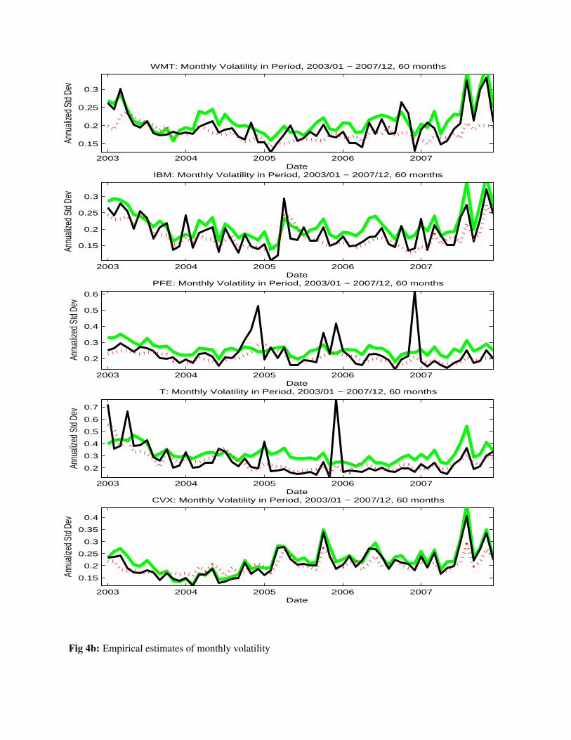
We estimate the monthly volatilities for the ten stocks in our sample. Figure 4 plots the estimates
over the sample period. To avoid jamming the figures, only the estimates VA3 (for δ = 0.25%), VR and
VG are presented. It can be seen that all estimates track each other quite closely, and there does not
appear to be any systematic bias among the different methods. The RV method, however, exhibits a few
extreme values of high volatility estimates and generally have the largest fluctuations among the three
methods. It is interesting to observe that the volatility paths of the different stocks show significant
co-movements.
Table 5 summarizes the pairwise correlation coefficients of the volatility estimates VA3, VR and
VG for the ten stocks. It can be seen that the correlations are highest for VA3, followed by VG and
then VR. Of the 45 pairs of correlations 93.3% are maximized when VA3 is used as the volatility
estimate, the remaining 6.7% are maximized when VG is used as the volatility estimate, with none for6Results for alternative model parameters for robustness check are similar. These results are not presented here, but
can be obtained from the authors on request.
10
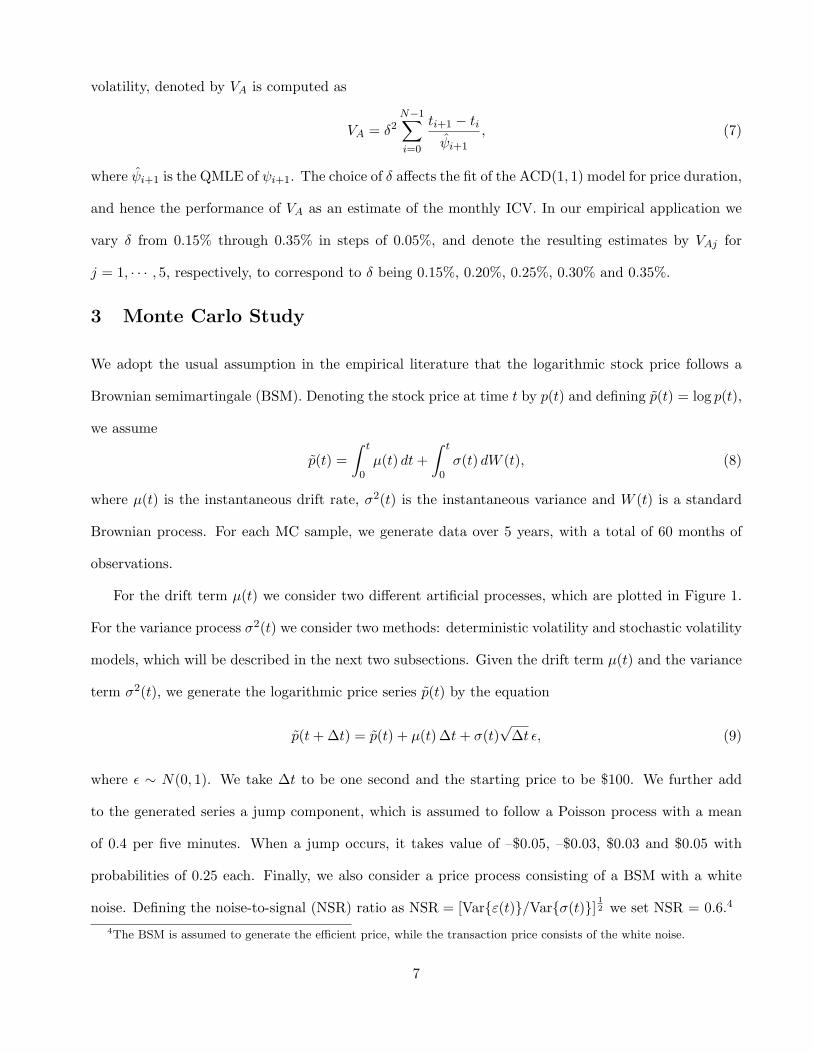
VR. Many studies in the literature examine the effects of macroeconomic variables on stock volatility,
and generally points to the co-movements of volatility across stocks. The ACD-ICV estimates support
a higher volatility co-movement versus estimates based on the RV method. It will be interesting to
further investigate volatility co-movements using the ACD-ICV estimates, in particular in relation to
macroeconomic variables such as inflation, exchange rate, GDP growth and interest-rate movements.
5 Volatility of S&P500
Implied volatility computed from option prices has often been used as a predictor for future historical
volatility. The S&P500 Index volatility has been a case of particular research interest in the literature
due to the popular reference to the CBOE volatility index VIX. Whaley (2009) provided a description
of VIX and discussed some of its properties. In this section we examine the use of VIX as a predictor for
future historical volatility when RV, GARCH and ACD-ICV estimates are used as proxies for historical
volatility.
VIX is calculated and disseminated in real time by CBOE. It is a forward-looking index of the
expected return volatility of the S&P500 Index over the next 30 calendar days and is implied from
the prices of S&P500 Index options. VIX is quoted in percentage points as the annualized standard
deviation of the return of the S&P500 Index over the next 30 days. It is based upon a model-free formula
using a wide range of selected near- and near-term put and call options. Studies in the literature on the
forecasting performance of implied volatility often use RV as the proxy for historical volatility. Jiang
and Tian (2005) and Becker, Clements and White (2007) used RV computed over 30-day intervals as
proxy for 30-day historical volatility in their studies on the information content of VIX on the volatility
of the S&P500. Recently, Chung, Tsai, Wang and Weng (2011) considered both VIX and VIX options
as predictors for the RV of the S&P500, although they did not specify the RV method used. We shall
investigate the forecasting performance of VIX for the volatility of S&P500 when historical volatility is
estimated by GARCH and ACD-ICV, and compare the results against using RV.
We downloaded daily closing values of VIX from the website of the CBOE. S&P500 tick data
were obtained from The Institute for Financial Markets (IFM) Data Center. 5-min S&P500 data were
11
extracted from 8:30 to 15:00 (Chicago time) each day. The sample period is from 1998 through 2007,
with 2516 daily observations.
We select N time points in the sample period that are at least 30 calendar days apart and denote
them by ti, for i = 1, · · · , N . Altogether there are 117 nonoverlapping 30-day intervals in our sample
(N = 117). Let VIXi be the closing value of VIX on day ti. We denote Yi as an estimate of the
historical volatility over the 30-day period starting from time ti, and consider the following regressions
of historical volatility estimates on volatility forecasts using VIX
Yi = α+ βVIXi + ξi, (14)
and
Y 2i = α+ βVIX2
i + ξi, (15)
for i = 1, · · · , N. The results are summarized in Table 6. It can be seen that the highest R2 is
for the regressions with the ACD-ICV measures as the dependent variables. Rather remarkably, the
regressions with VR as the dependent variable produce the lowest R2. The results show that VIX is a
more successful predictor of future volatility if volatility is estimated by the ACD-ICV method, but not
the RV method. Figure 5 plots VIX and some historical volatility estimates. There are some periods
for which VIX over-predicts volatility as estimated by VR. This over-prediction, however, is not evident
if historical volatility is estimated by the ACD-ICV method. Overall, our results show that VIX has
higher prediction value if its performance is measured against historical estimates using the ACD-ICV
method.
6 Conclusion
In this paper we extend the ACD-ICV method proposed by Tse and Yang (2011) to estimate stock
volatility over longer intervals such as a month. Estimation of low-frequency volatility is important
for studies involving macroeconomic data that are available only monthly or quarterly. As returns
over longer intervals are less susceptible to the contamination of noise over short intervals they may
be preferred in studies on asset pricing. Our MC study suggests that price events defined by return
12

thresholds of about 0.15% to 0.35% are appropriate for the ACD-ICV method. Based on the transaction
data, the ACD-ICV method outperforms the RV method in our MC experiments. On the other hand,
if daily data are used, the GARCH method based on aggregating the daily estimates of the conditional
variance is superior to the RV method, which is widely used in the literature.
Our empirical results using ten NYSE stocks show that the ACD-ICV, RV and GARCH estimates
track each other quite closely. The RV estimates, however, have larger fluctuations and exhibit oc-
casionally extreme volatility estimates. Co-movements of volatility across different stocks are highest
according to the ACD-ICV estimates. Our empirical study on VIX and the S&P500 index shows that
VIX is a more successful predictor of future volatility if volatility is estimated by the ACD-ICV method
than by the RV method. Overall we have shown that using the ACD-ICV method on high-frequency data
(tick transaction data) provides superior estimates of low-frequency volatility (over monthly intervals)
to the RV method.
References
[1] Aı̈t-Sahalia, Y., and L. Mancini, 2008, Out of sample forecasts of quadratic variation, Journal of
Econometrics, 147, 17-33.
[2] Andersen, T.G., T. Bollerslev, F.X. Diebold, and H. Ebens, 2001, The distribution of Realized
volatility, Journal of Financial Economics, 61, 43-76.
[3] Andersen, T.G., T. Bollerslev, F.X. Diebold, and P. Labys, 2001, The distribution of exchange rate
volatility, Journal of American Statistical Assoction, 96, 42-55.
[4] Bali, T.G., N. Cakici, X.S. Yan, and Z. Zhang, 2005, Does idiosyncratic risk really matter? Journal
of Finance, 60, 905-929.
[5] Becker, R., A.E. Clements, and S.I. White, 2007, Does implied volatility provide any information
beyond that captured in model-based volatility forecasts? Journal of Banking and Finance, 31,
2535-2549.
13
[6] Bollerslev, T., 1986, Generalized autoregressive conditional heteroskedasticity, Journal of Econo-
metrics, 31, 307-327.
[7] Chung, S.L., W.C. Tsai, Y.H. Wang, and P.S. Weng, 2011, The information content of the S&P500
index and VIX options on the dynamics of the S&P500 index, working paper, 21st Asia-Pacific
Futures Research Symposium.
[8] Engle, R.F., 1982, Autoregressive conditional heteroscedasticity with estimates of the variance of
United Kingdom inflation, Econometrica, 50, 987-1007.
[9] Engle, R.F., and J.R. Russell, 1998, Autoregressive conditional duration: A new model for irregu-
larly spaced transaction data, Econometrica, 66, 1127-1162.
[10] Fama, E.F., 1976, Inflation uncertainty and expected returns on Treasury bills, Journal of Political
Economy, 84, 427-448.
[11] Fernandes, M., and J. Grammig, 2006, A family of autoregressive conditional duration models,
Journal of Econometrics, 130, 1-23.
[12] French, K.R., G.W. Schwert, and R.F. Stambaugh, 1987, Expected stock returns and volatility,
Journal of Financial Economics, 19, 3-29.
[13] Fu, F., 2009, Idiosyncratic risk and the cross-section of expected stock returns, Journal of Financial
Economics, 91, 24-37.
[14] Goyal, A., and P. Santa-Clara, 2003, Idiosyncratic risk matters! Journal of Fiance, 58, 975-1007.
[15] Guo, H., and R. Savickas, 2008, Average idiosyncratic volatility in G7 countries, Reviews of Finan-
cial Studies, 21, 1259-1296.
[16] Heston, S.L., 1993, A closed-form solution for options with stochastic volatility with application to
bond and currency options, Review of Financial Studies, 6, 327-343.
[17] Jiang, G.J., and Y.S. Tian, 2005, The model-free implied volatility and its information content,
Review of Financial Studies, 18, 1305-1342.
14

[18] Jiang, G.J., and Y.S. Tian, 2010, Forecasting volatility using long memory and comovements: An
application to option valuation under SFAF 123R, Journal of Financial and Quantitative Analysis,
45, 502-533.
[19] Ludvigson, S.C., and S. Ng, 2007, The empirical risk-return relation: A factor analysis approach,
Journal of Financial Economics, 83, 171-222.
[20] Merton, R.C., 1980, On estimating the expected return on the market: An exploratory investiga-
tion, Journal of Financial Economics, 8, 323-361.
[21] Nelson, D.B., 1991, Conditional heteroskedasticity in assert returns: a new approach, Economet-
rica, 59, 347-370.
[22] Officer, R., 1973, The variability of the market factor of the New York Stock Exchange, Journal of
Business, 46, 434-454.
[23] Schwert, G.M., 1989, Why does stock market volatility change over time? Journal of Finance, 44,
1115-1153.
[24] Schwert, G.M., 1990a, Stock market volatility, Financial Analysts Journal, 46, 23-34.
[25] Schwert, G.M., 1990b, Stock Volatility and the Crash of ’87, Review of Financial studies, 3, 77-102.
[26] Schwert, G.M., and P.J. Seguin, 1990, Heteroskedasticity in stock returns, Journal of Finance, 45,
1129-1155.
[27] Tse, Y.K., and T. Yang, 2011, Estimation of high-frequency volatility: An autoregressive condi-
tional duration approach, working paper, Singapore Management University.
[28] Whaley, R.E., 2009, Understanding the VIX, Journal of Portfolio Management, 35, 98-105.
[29] Zhang, C., 2010, A Reexamination of the Causes of Time-Varying Stock Return Volatilities, Journal
of Financial and Quantitative Analysis, 45, 663-684.
15

Table 1: Monte Carlo results without overnight jumps.
Volatility ModelMV1 MV2 SV1 SV2 SV3
method ME RMSE ME RMSE ME RMSE ME RMSE ME RMSE
Panel A: Drift Model 1
VA1 0.538 0.654 0.578 0.681 0.894 1.115 0.839 1.061 0.816 1.041VA3 0.350 0.603 0.377 0.596 0.616 0.994 0.599 0.977 0.624 0.990VA5 0.272 0.669 0.298 0.639 0.507 1.060 0.540 1.089 0.587 1.131VR 0.043 0.272 0.034 0.325 0.025 0.519 0.028 0.486 0.031 0.466VD -0.514 2.395 -0.624 2.892 -1.037 4.675 -0.957 4.358 -0.906 4.165VG 0.133 1.745 0.191 1.916 0.446 3.769 0.535 3.797 0.654 3.825
Panel B: Drift Model 2
VA1 0.554 0.666 0.596 0.699 0.949 1.172 0.882 1.106 0.856 1.080VA3 0.356 0.607 0.387 0.604 0.654 1.030 0.631 1.007 0.655 1.018VA5 0.286 0.673 0.306 0.643 0.534 1.091 0.562 1.109 0.606 1.149VR 0.044 0.272 0.035 0.325 0.026 0.520 0.029 0.486 0.032 0.466VD -0.514 2.395 -0.624 2.892 -1.037 4.675 -0.957 4.358 -0.906 4.165VG 0.133 1.747 0.203 1.915 0.446 3.768 0.536 3.797 0.656 3.825
Notes: ME = mean error, RMSE = root mean-squared error. The results are based on 1000 MC replications of 5-year monthlyvolatility. All figures are annualized standard deviation in percentage. VA1, VA3 and VA5 are the ACD-ICV volatility estimateswith δ = 0.15%, 0.25% and 0.35%, respectively. VR and VD are the realized volatility estimates computed using 5-min and dailyreturns, respectively. VG is the GARCH estimate based on daily data.
Table 2: Monte Carlo results with overnight jumps following the Generalized Normal Distribution
Volatility ModelMV1 MV2 SV1 SV2 SV3
method ME RMSE ME RMSE ME RMSE ME RMSE ME RMSE
Panel A: Drift Model 1
VA1 0.249 1.890 0.502 1.321 0.827 1.659 0.606 1.850 0.424 2.061VA3 0.006 1.892 0.227 1.280 0.406 1.513 0.218 1.762 0.077 2.046VA5 -0.077 1.849 0.111 1.288 0.237 1.526 0.106 1.820 0.024 2.085VR -0.182 2.860 -0.124 2.563 -0.066 2.026 -0.087 2.164 -0.104 2.273VD -0.885 4.042 -0.919 4.211 -1.224 5.403 -1.170 5.170 -1.138 5.039VG 0.436 2.328 0.390 2.301 0.330 3.808 0.349 3.864 0.385 3.927
Panel B: Drift Model 2
VA1 0.274 1.895 0.530 1.327 0.904 1.735 0.672 1.901 0.485 2.103VA3 0.020 1.889 0.243 1.279 0.459 1.562 0.263 1.795 0.116 2.070VA5 -0.069 1.847 0.121 1.285 0.275 1.558 0.139 1.845 0.050 2.104VR -0.181 2.860 -0.123 2.563 -0.064 2.026 -0.086 2.164 -0.103 2.272VD -0.884 4.042 -0.919 4.211 -1.224 5.403 -1.169 5.170 -1.138 5.039VG 0.439 2.327 0.413 2.329 0.327 3.804 0.350 3.863 0.385 3.926
Notes: ME = mean error, RMSE = root mean-squared error. The results are based on 1000 MC replications of 5-year monthlyvolatility. All figures are annualized standard deviation in percentage. VA1, VA3 and VA5 are the ACD-ICV volatility estimateswith δ = 0.15%, 0.25% and 0.35%, respectively. VR and VD are the realized volatility estimates computed using 5-min and dailyreturns, respectively. VG is the GARCH estimate based on daily data.

Table 3: Monte Carlo results with overnight jumps following the t Distribution
Volatility ModelMV1 MV2 SV1 SV2 SV3
method ME RMSE ME RMSE ME RMSE ME RMSE ME RMSE
Panel A: Drift Model 1
VA1 -1.165 2.106 -0.767 1.402 -0.065 1.496 -0.341 1.779 -0.562 2.061VA3 -1.411 2.256 -1.041 1.581 -0.484 1.558 -0.732 1.872 -0.913 2.179VA5 -1.493 2.274 -1.154 1.670 -0.659 1.648 -0.846 1.962 -0.974 2.230VR -1.705 3.537 -1.456 3.145 -1.038 2.462 -1.143 2.647 -1.225 2.791VD -2.369 4.685 -2.215 4.717 -2.167 5.716 -2.197 5.534 -2.230 5.443VG -1.092 2.460 -0.905 2.405 -0.595 3.759 -0.654 3.801 -0.680 3.847
Panel B: Drift Model 2
VA1 -1.143 2.094 -0.741 1.380 0.011 1.552 -0.276 1.818 -0.502 2.082VA3 -1.398 2.246 -1.027 1.570 -0.432 1.591 -0.687 1.891 -0.874 2.188VA5 -1.484 2.269 -1.146 1.661 -0.617 1.669 -0.813 1.976 -0.945 2.238VR -1.704 3.537 -1.455 3.144 -1.037 2.462 -1.142 2.646 -1.224 2.790VD -2.369 4.685 -2.215 4.717 -2.167 5.716 -2.196 5.534 -2.231 5.443VG -1.116 2.469 -0.922 2.398 -0.595 3.758 -0.657 3.799 -0.680 3.845
Notes: ME = mean error, RMSE = root mean-squared error. The results are based on 1000 MC replications of 5-year monthlyvolatility. All figures are annualized standard deviation in percentage. VA1, VA3 and VA5 are the ACD-ICV volatility estimateswith δ = 0.15%, 0.25% and 0.35%, respectively. VR and VD are the realized volatility estimates computed using 5-min and dailyreturns, respectively. VG is the GARCH estimate based on daily data.
Table 4: Monte Carlo results with overnight jumps randomly drawn from the empirical jumps
Volatility ModelMV1 MV2 SV1 SV2 SV3
method ME RMSE ME RMSE ME RMSE ME RMSE ME RMSE
Panel A: Drift model 1
VA1 0.240 1.939 0.487 1.377 0.729 1.608 0.524 1.828 0.356 2.060VA3 0.012 1.930 0.226 1.330 0.349 1.506 0.176 1.773 0.039 2.054VA5 -0.065 1.880 0.120 1.333 0.195 1.534 0.081 1.838 0.001 2.097VR -0.286 3.459 -0.200 3.142 -0.099 2.509 -0.127 2.667 -0.150 2.788VD -0.986 4.525 -0.994 4.633 -1.256 5.663 -1.209 5.464 -1.184 5.358VG 0.369 2.359 0.386 2.341 0.342 3.862 0.357 3.923 0.387 3.993
Panel B: Drift model 2
VA1 0.263 1.944 0.513 1.375 0.791 1.665 0.577 1.870 0.403 2.092VA3 0.022 1.932 0.238 1.331 0.393 1.546 0.208 1.801 0.070 2.076VA5 -0.055 1.878 0.129 1.332 0.229 1.558 0.106 1.855 0.021 2.112VR1 -0.285 3.459 -0.200 3.142 -0.098 2.509 -0.126 2.667 -0.149 2.788VD -0.986 4.525 -0.994 4.632 -1.256 5.663 -1.209 5.465 -1.185 5.358VG 0.327 2.332 0.407 2.369 0.341 3.861 0.357 3.922 0.387 3.992
Notes: ME = mean error, RMSE = root mean-squared error. The results are based on 1000 MC replications of 5-year monthlyvolatility. All figures are annualized standard deviation in percentage. VA1, VA3 and VA5 are the ACD-ICV volatility estimateswith δ = 0.15%, 0.25% and 0.35%, respectively. VR and VD are the realized volatility estimates computed using 5-min and dailyreturns, respectively. VG is the GARCH estimate based on daily data.
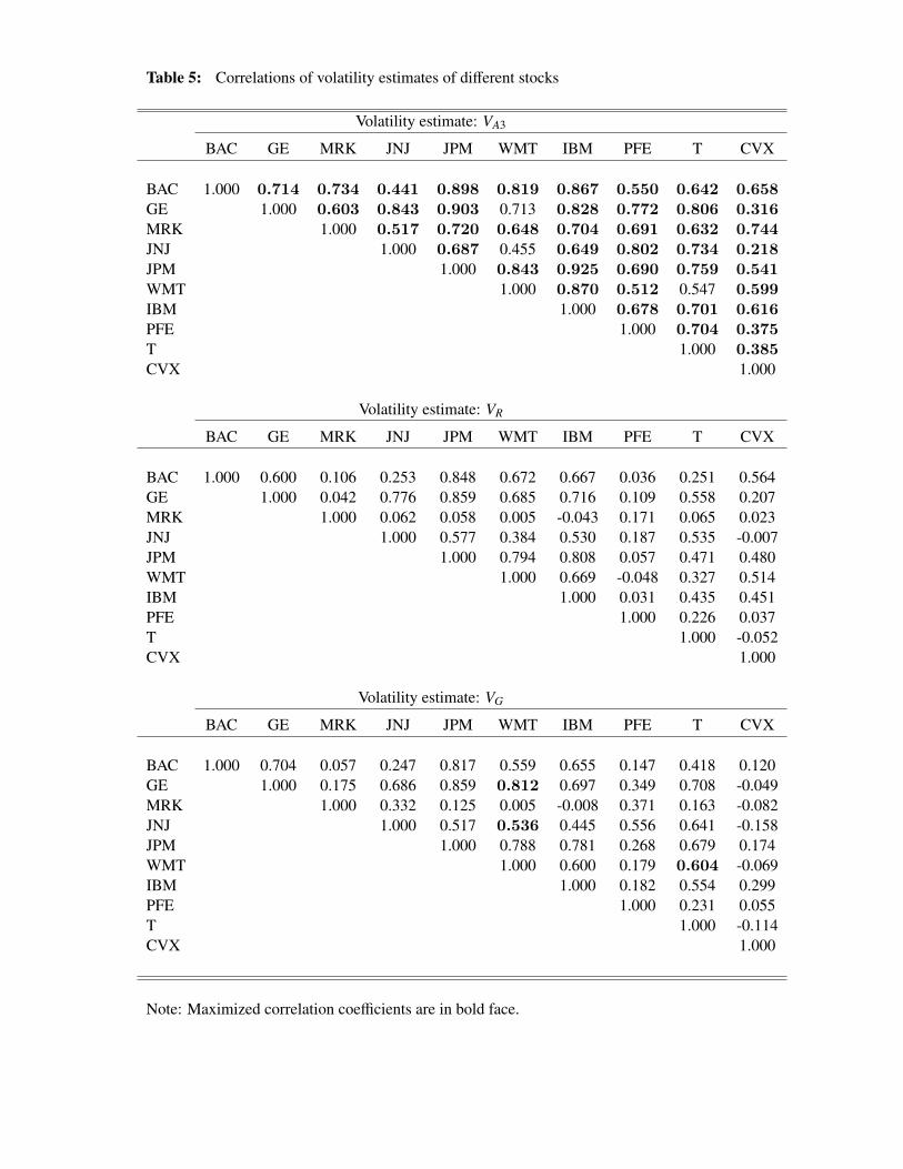
Table 5: Correlations of volatility estimates of different stocks
Volatility estimate: VA3
BAC GE MRK JNJ JPM WMT IBM PFE T CVX
BAC 1.000 0.714 0.734 0.441 0.898 0.819 0.867 0.550 0.642 0.658GE 1.000 0.603 0.843 0.903 0.713 0.828 0.772 0.806 0.316MRK 1.000 0.517 0.720 0.648 0.704 0.691 0.632 0.744JNJ 1.000 0.687 0.455 0.649 0.802 0.734 0.218JPM 1.000 0.843 0.925 0.690 0.759 0.541WMT 1.000 0.870 0.512 0.547 0.599IBM 1.000 0.678 0.701 0.616PFE 1.000 0.704 0.375T 1.000 0.385CVX 1.000
Volatility estimate: VR
BAC GE MRK JNJ JPM WMT IBM PFE T CVX
BAC 1.000 0.600 0.106 0.253 0.848 0.672 0.667 0.036 0.251 0.564GE 1.000 0.042 0.776 0.859 0.685 0.716 0.109 0.558 0.207MRK 1.000 0.062 0.058 0.005 -0.043 0.171 0.065 0.023JNJ 1.000 0.577 0.384 0.530 0.187 0.535 -0.007JPM 1.000 0.794 0.808 0.057 0.471 0.480WMT 1.000 0.669 -0.048 0.327 0.514IBM 1.000 0.031 0.435 0.451PFE 1.000 0.226 0.037T 1.000 -0.052CVX 1.000
Volatility estimate: VG
BAC GE MRK JNJ JPM WMT IBM PFE T CVX
BAC 1.000 0.704 0.057 0.247 0.817 0.559 0.655 0.147 0.418 0.120GE 1.000 0.175 0.686 0.859 0.812 0.697 0.349 0.708 -0.049MRK 1.000 0.332 0.125 0.005 -0.008 0.371 0.163 -0.082JNJ 1.000 0.517 0.536 0.445 0.556 0.641 -0.158JPM 1.000 0.788 0.781 0.268 0.679 0.174WMT 1.000 0.600 0.179 0.604 -0.069IBM 1.000 0.182 0.554 0.299PFE 1.000 0.231 0.055T 1.000 -0.114CVX 1.000
Note: Maximized correlation coefficients are in bold face.
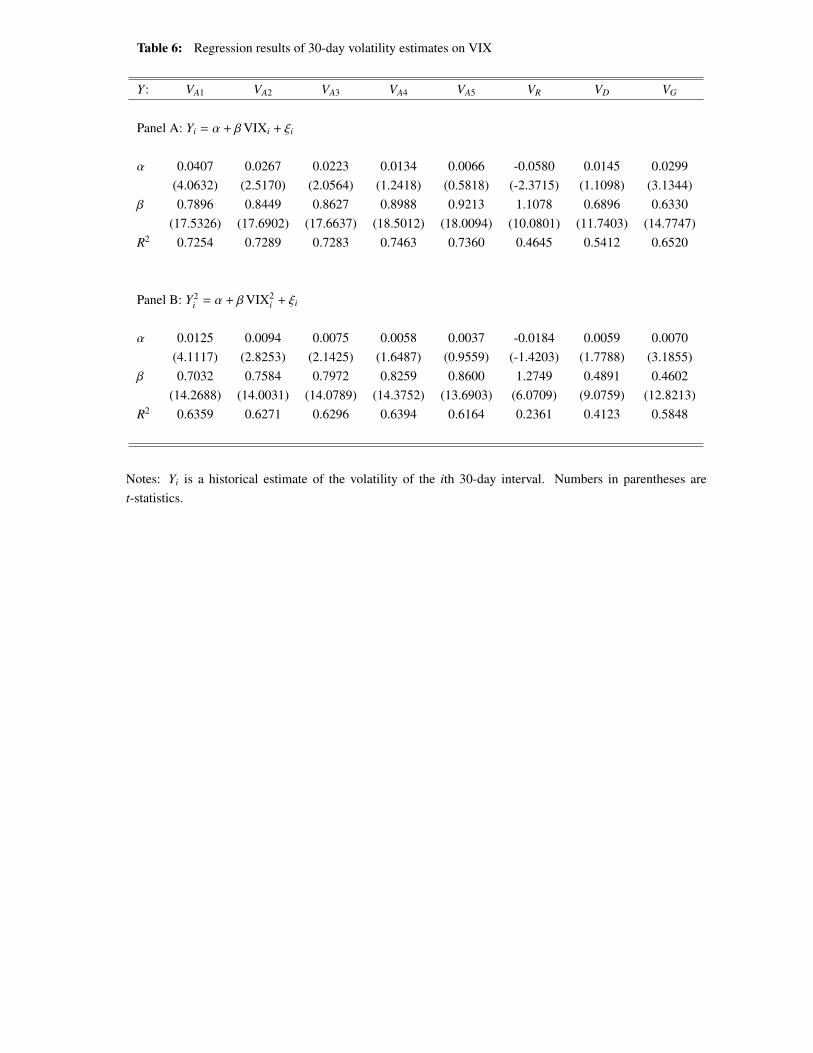
Table 6: Regression results of 30-day volatility estimates on VIX
Y: VA1 VA2 VA3 VA4 VA5 VR VD VG
Panel A: Yi = α + βVIXi + ξi
α 0.0407 0.0267 0.0223 0.0134 0.0066 -0.0580 0.0145 0.0299(4.0632) (2.5170) (2.0564) (1.2418) (0.5818) (-2.3715) (1.1098) (3.1344)
β 0.7896 0.8449 0.8627 0.8988 0.9213 1.1078 0.6896 0.6330(17.5326) (17.6902) (17.6637) (18.5012) (18.0094) (10.0801) (11.7403) (14.7747)
R2 0.7254 0.7289 0.7283 0.7463 0.7360 0.4645 0.5412 0.6520
Panel B: Y2i = α + βVIX2
i + ξi
α 0.0125 0.0094 0.0075 0.0058 0.0037 -0.0184 0.0059 0.0070(4.1117) (2.8253) (2.1425) (1.6487) (0.9559) (-1.4203) (1.7788) (3.1855)
β 0.7032 0.7584 0.7972 0.8259 0.8600 1.2749 0.4891 0.4602(14.2688) (14.0031) (14.0789) (14.3752) (13.6903) (6.0709) (9.0759) (12.8213)
R2 0.6359 0.6271 0.6296 0.6394 0.6164 0.2361 0.4123 0.5848
Notes: Yi is a historical estimate of the volatility of the ith 30-day interval. Numbers in parentheses aret-statistics.

1 12 24 36 48 60
−303
8
Period in Month
Drif
t (%
per
yea
r)
Drift Model 2
1 12 24 36 48 600
5
10
Period in Month
Drif
t (%
per
yea
r)
Drift Model 1
Figure 1: The drift term
1 12 24 36 48 60
0.1
0.15
0.2
Period in Month
Ann
ualiz
ed S
td D
ev
DV Model 1
1 12 24 36 48 60
0.1
0.15
0.2
0.25
Period in Month
Ann
ualiz
ed S
td D
ev
DV Model 2
Figure 2: Deterministic volatility models

1 12 24 36 48 600.1
0.2
0.3
0.4
0.5
0.6
Period in Month
Ann
ualiz
ed S
tand
ard
Dev
iatio
nSV Model 1: Monthly volatility estimates
V
A3
VR
VG
True Vol
1 12 24 36 48 600.1
0.2
0.3
0.4
0.5
0.6
Period in Month
Ann
ualiz
ed S
tand
ard
Dev
iatio
n
SV Model 2: Monthly volatility estimates
1 12 24 36 48 600.1
0.2
0.3
0.4
0.5
0.6
Period in Month
Ann
ualiz
ed S
tand
ard
Dev
iatio
n
SV Model 3: Monthly volatility estimates
Figure 3: Estimation of stochastic volatility with empirical overnight price jumps

2003 2004 2005 2006 2007
0.2
0.3
0.4
Date
Annu
alize
d Std
Dev
BAC: Monthly Volatility in Period, 2003/01 − 2007/12, 60 months
VA3
VR
VG
2003 2004 2005 2006 2007
0.15
0.2
0.25
0.3
0.35
Date
Annu
alize
d Std
Dev
GE: Monthly Volatility in Period, 2003/01 − 2007/12, 60 months
2003 2004 2005 2006 2007
0.2
0.4
0.6
0.8
1
Date
Annu
alize
d Std
Dev
MRK: Monthly Volatility in Period, 2003/01 − 2007/12, 60 months
2003 2004 2005 2006 2007
0.1
0.15
0.2
0.25
0.3
Date
Annu
alize
d Std
Dev
JNJ: Monthly Volatility in Period, 2003/01 − 2007/12, 60 months
2003 2004 2005 2006 2007
0.2
0.3
0.4
0.5
Date
Annu
alize
d Std
Dev
JPM: Monthly Volatility in Period, 2003/01 − 2007/12, 60 months
Fig 4a: Empirical estimates of monthly volatility
2003 2004 2005 2006 2007
0.15
0.2
0.25
0.3
Date
Annu
alize
d Std
Dev
WMT: Monthly Volatility in Period, 2003/01 − 2007/12, 60 months
2003 2004 2005 2006 2007
0.15
0.2
0.25
0.3
Date
Annu
alize
d Std
Dev
IBM: Monthly Volatility in Period, 2003/01 − 2007/12, 60 months
2003 2004 2005 2006 2007
0.2
0.3
0.4
0.5
0.6
Date
Annu
alize
d Std
Dev
PFE: Monthly Volatility in Period, 2003/01 − 2007/12, 60 months
2003 2004 2005 2006 2007
0.2
0.3
0.4
0.5
0.6
0.7
Date
Annu
alize
d Std
Dev
T: Monthly Volatility in Period, 2003/01 − 2007/12, 60 months
2003 2004 2005 2006 2007
0.15
0.2
0.25
0.3
0.35
0.4
Date
Annu
alize
d Std
Dev
CVX: Monthly Volatility in Period, 2003/01 − 2007/12, 60 months
Fig 4b: Empirical estimates of monthly volatility

10 20 30 40 50 60 70 80 90 100 1100
0.1
0.2
0.3
0.4
0.5
0.6
0.7
0.8
0.9
30−day interval in period 1988 through 2007
Ann
ualiz
ed S
tand
ard
Dev
iatio
n
30−day volatility, 1988/01 − 2007/12,117periods
V
A3
VR
VG
VIX
Figure 5: VIX and S&P500 30-day volatility estimates