Harvest Contract Price Volatility for Cotton

Darren Hudson and Keith Coble

The authors are Assistant Professors, Department of Agricultural Economics, MississippiState University. The comments of Lanny Bateman, O.A. Cleveland, Warren Couvillion,Patrick Gerard, and Bill Herndon on an earlier version of this paper are appreciated. Mississippi Agricultural and Forestry Experiment Station Paper (in press).

1

Harvest Contract Price Volatility for Cotton

Introduction

Changes in farm and international trade policy have increased attention to issues of

risk management. There is a variety of literature on different components of risk

management schemes. One line of literature has been in the area of crop insurance. Coble

provides a synthesis of some of this literature, especially yield risk insurance. The major

thrust of this line of research is the ability of various insurance products to shift various

risks as well as the effect of insurance on producer decisions.

Another vein of literature focuses on forward pricing decisions. Of particular

interest is how producers and other market participants may reduce price risk using these

instruments. Early work by Feder, Just, and Schmitz examined a futures market without

basis or production risk and unbiased price expectations. They found a “separation” result

that led to hedging expected production and was not conditioned on price variability.

More general models which include production risk (McKinnon; Grant) find the optimal

hedging level is conditional on price variability, as do models which include basis risk

(Benniga, Eldo, and Zilcha; Heifner, 1973; Kahl). These results first found under the

limiting assumptions of mean-variance analysis have generally held in the less restrictive

expected utility framework (Lapan and Moschini). Optimal hedge ratios are implicitly

driven by the volatility of futures prices (Lence and Hayes). It has also been shown that

options, which derive value from the volatility of the underlying futures price, can be a

2

part of a producer’s optimal price risk management scheme (Sakong, Hayes, and Hallam;

Moschini and Lapan). Given these findings, the volatility of futures prices is of

importance to producers and other market participants.

There are many factors that are believed to affect the volatility of futures prices

(Anderson; Kenyon et al.; Hennesey and Wahl; Streeter and Tomek). These include

weather factors, the time left to maturity of the contract, as well as decision variables such

as planting time (acreage allocation), the level of futures prices, and government policy

variables. There is an abundance of literature on price volatilities in major commodities

such as corn, wheat and soybeans. However, there has been little work in cotton.

Cotton price volatility is expected to respond to many of the same factors as

grains, but there are some unique factors of cotton production that may affect volatility

differently. For example, cotton production occurs across the entire southern United

States in contrast to the relatively concentrated production of corn in the Midwest. This

may serve to dampen some of the effects of anomalous weather events in one particular

region. That is, cotton may be heat stressed in California, but good growing conditions

may exist in Texas, the Delta, and the Southeast so that no significant increase in volatility

may occur. Additionally, cotton production is globally dispersed. The U.S. is a major

producer of cotton, but not to the extent that it is a major producer of corn (the U.S.

produced 46.2% of world corn production in 1994 compared to 23% of world cotton

production). Thus, events that occur within the U.S. cotton market may have less impact

on price volatility compared to food and feed grains, ceteris paribus.

1 The harvest contract in this case is the December contract. The Octobercontract can also be considered a harvest contract, but it is thinly traded as compared toDecember. Thus, this analysis is limited to the December contract.

3

Understanding price volatility is important for several reasons. Early concerns

were that the Federal Agricultural Improvement and Reform (FAIR) Act of 1996 would

increase volatility of prices. Recent work by Ray et al., however, does not suggest this

will happen for cotton. Understanding what has affected volatility may give indications

about what to expect in the future. Thus, the objective of this paper is to examine price

volatilities in cotton, focusing on the growing season volatility of the harvest contract.1

Price Volatility

The growing season volatility of the harvest contract was selected for two reasons.

First, information about the crop is limited prior to planting, thus limiting price volatility

(assuming no shocks in demand). Confining the sample period from planting to harvest

should eliminate seasonal variation in volatilities attributable to pre-planting lack of

volatility. Second, growing season volatility is of particular interest to cotton producers

because many of their marketing decisions are usually made during this period. At the

same time, the harvest contract is used by other market participants to begin pricing

cotton for delivery to their mills or warehouses.

Growing season was defined for this analysis as the period between May 1 and the

close of the December contract for each year. On average in the U.S., cotton planting is

4

over half completed by the end of May and harvest is essentially complete by the close of

the December contract (NASS). Thus, this seven month period should isolate volatility to

that which occurs within the growing season.

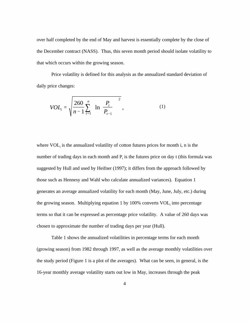
Price volatility is defined for this analysis as the annualized standard deviation of

daily price changes:

VOLn

P

Pit

tt

n

=−

−=∑260

1 1

2

1

ln , (1)

where VOLi is the annualized volatility of cotton futures prices for month i, n is the

number of trading days in each month and Pt is the futures price on day t (this formula was

suggested by Hull and used by Heifner (1997); it differs from the approach followed by

those such as Hennesy and Wahl who calculate annualized variances). Equation 1

generates an average annualized volatility for each month (May, June, July, etc.) during

the growing season. Multiplying equation 1 by 100% converts VOLi into percentage

terms so that it can be expressed as percentage price volatility. A value of 260 days was

chosen to approximate the number of trading days per year (Hull).

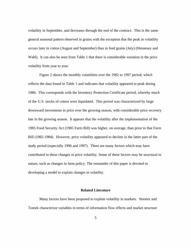
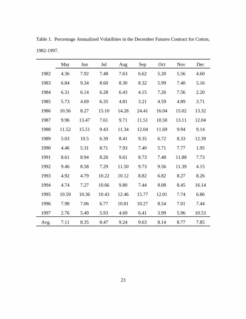
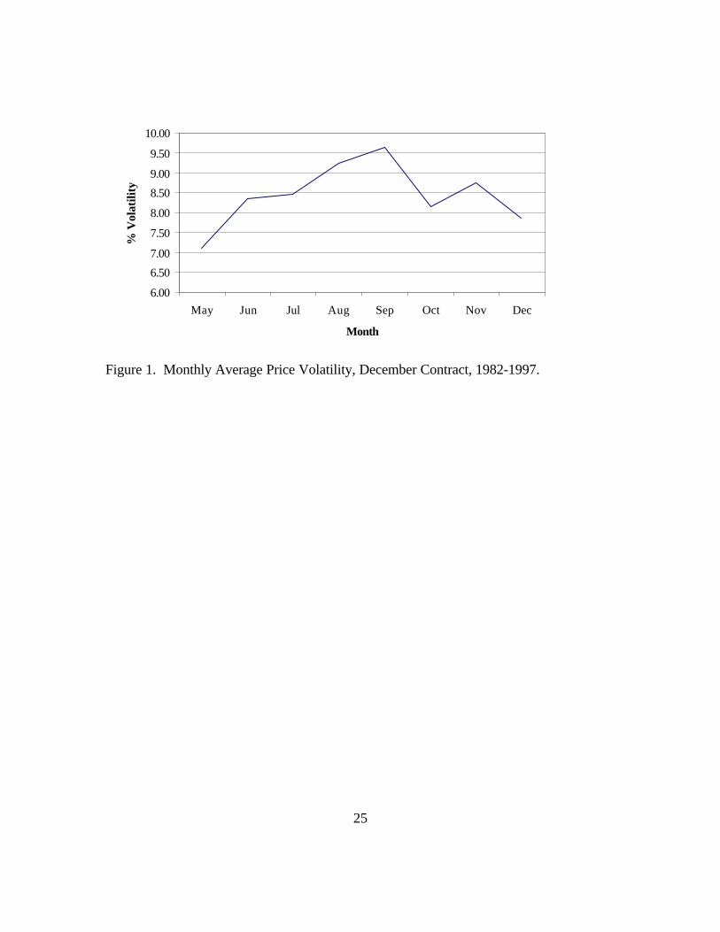
Table 1 shows the annualized volatilities in percentage terms for each month

(growing season) from 1982 through 1997, as well as the average monthly volatilities over

the study period (Figure 1 is a plot of the averages). What can be seen, in general, is the

16-year monthly average volatility starts out low in May, increases through the peak

5

volatility in September, and decreases through the end of the contract. This is the same

general seasonal pattern observed in grains with the exception that the peak in volatility

occurs later in cotton (August and September) than in feed grains (July) (Hennesey and

Wahl). It can also be seen from Table 1 that there is considerable variation in the price

volatility from year to year.

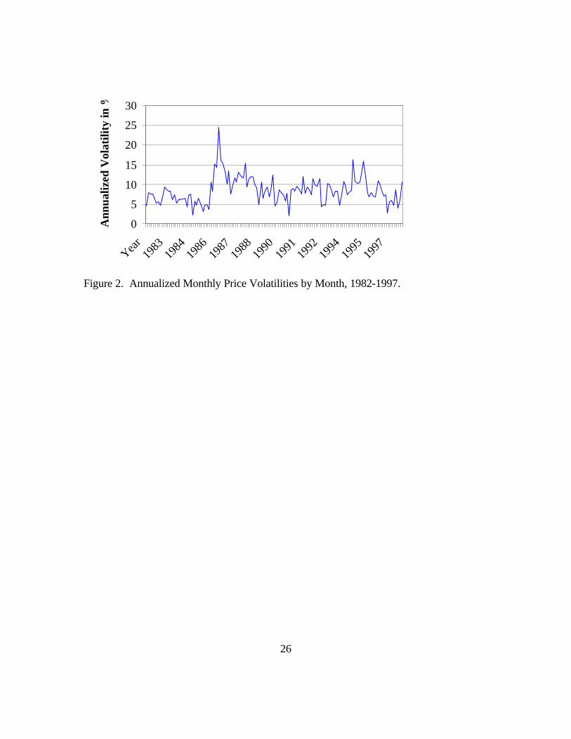
Figure 2 shows the monthly volatilities over the 1982 to 1997 period, which

reflects the data found in Table 1 and indicates that volatility appeared to peak during

1986. This corresponds with the Inventory Protection Certificate period, whereby much

of the U.S. stocks of cotton were liquidated. This period was characterized by large

downward movements in price over the growing season, with considerable price recovery

late in the growing season. It appears that the volatility after the implementation of the

1985 Food Security Act (1985 Farm Bill) was higher, on average, than prior to that Farm

Bill (1982-1984). However, price volatility appeared to decline in the latter part of the

study period (especially 1996 and 1997). There are many factors which may have

contributed to these changes in price volatility. Some of these factors may be structural in

nature, such as changes in farm policy. The remainder of this paper is devoted to

developing a model to explain changes in volatility.

Related Literature

Many factors have been proposed to explain volatility in markets. Streeter and

Tomek characterize variables in terms of information flow effects and market structure

6

effects. Information flow effects relate to those factors which increase or decrease the

amount of information in the marketplace. There are alternative ways that these

informational effects are expressed. Some authors examine the “time-to-maturity” effect

(e.g., Hennesey and Wahl; Samuelson) by specifying a variable composed of the number

of months to contract maturity. The underlying concept behind this variable is that

information about the crop will be more limited the farther in time from maturity. As time

progresses, more information comes into the market and prices become more volatile as

market participants work out the proper impact of this information on future

prices. Thus, volatility is expected to increase the closer to contract maturity, ceteris

paribus. This effect is sometimes called the “Samuelson hypothesis.”

Seasonal effects might also be called information effects. In critical times of crop

development, prices tend to become more volatile because of the uncertainty about crop

conditions. Market participants likely become acutely sensitive to new information during

these times. A common method for examining seasonal effects is the use of seasonal

dummy variables (e.g., Kenyon et al., Hennesey and Wahl). Streeter and Tomek, in

contrast, used a harmonic approach for addressing seasonality by adding a series of sine

and cosine variables to a regression on price volatility. The appealing feature of this

approach is that it allows for a continuous change in volatility versus the discrete changes

forced by the use of dummy variables. In the context of the current analysis, this approach

may not be viable because the period of interest is the growing

7

season. That is, truncating the sample period in the middle of the contract disrupts the

continuity, thus making it difficult to accurately specify the harmonic variables.

Literature also points to the importance of considering economic variables in

addition to the information variables (Kenyon et al.; Streeter and Tomek; Glauber and

Heifner). For example, both Kenyon et al. and Glauber and Heifner found a direct

relationship between the level of futures prices and price volatility. That is, as futures

prices increased, price volatility also tended to increase. This is not a surprising in that

higher prices have “more room to move” than lower prices, in general. Hennesey and

Wahl also found an important role for decision-making variables such as planting. Post-

planting volatilities appeared to be significantly higher than pre-planting volatilities, even

after controlling for other factors such as the time-to-maturity and weather.

The available body of literature provides some indication of variables that may

explain volatility. However, there is little work available on price volatility in cotton. The

lack of literature in cotton makes it difficult to identify variables that may be of importance

to cotton price volatilities. The following section presents a model, utilizing findings from

other commodities, which explores some of the factors that may be important for cotton

price volatility.

8

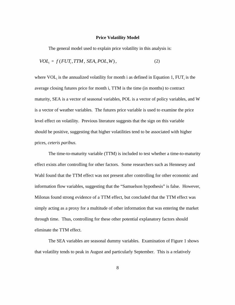
Price Volatility Model

The general model used to explain price volatility in this analysis is:

VOL f FUT TTM SEA POL Wi i= ( , , , , ) , (2)

where VOLi is the annualized volatility for month i as defined in Equation 1, FUTi is the

average closing futures price for month i, TTM is the time (in months) to contract

maturity, SEA is a vector of seasonal variables, POL is a vector of policy variables, and W

is a vector of weather variables. The futures price variable is used to examine the price

level effect on volatility. Previous literature suggests that the sign on this variable

should be positive, suggesting that higher volatilities tend to be associated with higher

prices, ceteris paribus.

The time-to-maturity variable (TTM) is included to test whether a time-to-maturity

effect exists after controlling for other factors. Some researchers such as Hennesey and

Wahl found that the TTM effect was not present after controlling for other economic and

information flow variables, suggesting that the “Samuelson hypothesis” is false. However,

Milonas found strong evidence of a TTM effect, but concluded that the TTM effect was

simply acting as a proxy for a multitude of other information that was entering the market

through time. Thus, controlling for these other potential explanatory factors should

eliminate the TTM effect.

The SEA variables are seasonal dummy variables. Examination of Figure 1 shows

that volatility tends to peak in August and particularly September. This is a relatively

9

important time in terms of crop development for cotton because if its need for heat units

to mature. Much of the yield may be determined during this period, which affects

volatility. This phenomenon of seasonality is not unique to cotton, but it quite common in

the other major agricultural commodities. Thus, two dummy variables were included in

the model–one for August and one for September (i.e., AUG=1 if August, 0 otherwise;

SEP=1 if September, 0 otherwise).

Another potentially important factor found in the literature is weather. Changes in

weather variables alter expectations about crop size, and thus, price. For this analysis, the

effects of rainfall and temperature are considered. Hennesey and Wahl considered the

absolute deviation of monthly rainfall and temperature from a long-term average in their

model of grain price volatility. A variation of that approach is adopted here. For rainfall:

% ln ,,

RainRain

ARaini t

i

=

(3)

where Raini,t is the weighted average (as described below) U.S. cotton belt rainfall for

month i during year t, and ARaini is the long-term (1895 to current period) weighted

average U.S. cotton belt rainfall for month i. One primary difference between cotton and

corn, for example, is that cotton is grown in a geographically dispersed area (from the east

coast to the west coast). To control for the potential variation across this broad area,

rainfall data was collected for three major producing areas (Mississippi, Texas, and

10

California). The monthly rainfall totals for each of these areas were weighted by each

state’s cotton production to generate a weighted average rainfall total. The long-term

weighted average rainfall was weighted in the same fashion. Equation 3 constructs a

variable that expresses the percentage difference between current month’s rainfall and the

long-term average for that month. A similar procedure was used to create variable for

temperature (%Temp).

The policy variables are the most difficult to define and operationalize. There were

three distinct changes in policy that occurred over the period of analysis (1982-1997). To

some extent, these three changes in policy were intermediate steps to a final goal. That is,

each set of farm legislation progressively moved in the direction of agriculture responding

more to market forces (Glade et al.). The first step during this period was the farm

legislation of 1985. A primary component of this legislation was the implementation of a

marketing loan program. This program paid the difference between the world price and

the U.S. price to exporters who wished to export U.S. cotton. This policy was

implemented in response to the fact that the U.S. price had persistently been above the

world price, limiting U.S. exports. This allowed stocks to be drawn down, thus

potentially increasing U.S. price responsiveness to changes in world prices.

A second element that occurred within the 1985 farm bill period was the Inventory

Protection Certificates. These certificates protected stock-holders of cotton from

downward price movements, which allowed prices to “fall through” the floor on prices set

by the loan rate. This program resulted in a dramatic increase in price volatility during the

2 Indeed, some are still asserting a long-term increase in volatility in grain markets(Ray et al.).

11

1986 crop year (Figure 2) as prices declined rapidly and then made a modest recovery.

Thus, the 1986 crop year is controlled for through the use of a dummy variable for 1986

(Y86=1 if 1986 and 0 otherwise). This should isolate the effects of the Inventory

Protection Certificates.

The second major shift in policy occurred in 1990 with the farm legislation enacted

that year. The marketing loan program was continued with slight modifications (Glade et

al.) and a move was made towards more planting flexibility. Mandatory acreage reduction

percentages were reduced after 1990, and a greater use of “flex” acres was implemented.

Finally, the 1996 farm legislation was the culmination of the movement to total

flexibility to the producer in terms of planting decisions. Market prices were then free to

be determined by market forces, with the exception of remaining trade restrictions. Early

debate was centered around the possibility that this shift in policy would lead to increased

volatility.2 However, Figure 2 reveals that an increase in volatility has yet to occur for

cotton. Reasons for this lack of volatility increase are explored later.

There are several difficulties in dealing with policy variables in a framework such

as the current study. First, policy changes are discrete in nature, which does not readily

lend itself to explaining price variations on a monthly basis. That is, markets likely

discount the information coming from policy variables before the crop year begins so that

policy variables likely explain year-to-year differences in price volatility rather than intra-

12

year price volatility. Second, there are elements within each farm bill that will tend to

increase volatility as well as elements that will tend to decrease volatility. It is difficult to

disaggregate the individual effects of these policies on monthly price volatility.

The simplest method of controlling for policy effects is to use dummy variables.

The limitations of the use of dummy variables are noted above. However, it seems

reasonable to expect that the existence of these policies have had some impact on price

volatility. The difficulty of confounding effects in a policy is not solved by utilizing

dummy variables. However, results using dummy variables are sufficiently generalizable

when correctly interpreted. Because of the potential for confounding effects, the

interpretation of the resulting parameter estimate on a policy dummy variable is that it is

the net effect of the policy on price volatility. This limits inferences that can be made from

those parameter estimates, but allows the controlling for the lump sum effects of those

policies.

The model, given the above, that was estimated was:

VOL f FUT TTM AUG SEP P

P P Y Rain Tempi i= ( , , , , ,

, , ,% ,% ) ,

85

90 96 86(4)

where P85, P90, and P96 are dummy variables for the 1985, 1990, and 1996 farm bills,

respectively (dummy=1 if during policy period, 0 otherwise). Data on daily closing prices

of each year’s December contract from 1982 through 1997 were collected and used to

calculate the average monthly annualized volatility using Equation 1. Weather data were

13

derived from the National Oceanographic and Atmospheric Administration’s (NOAA)

database, which contains monthly observations across all states starting, in most cases, in

1895. Equation 4 was estimated using Ordinary Least Squares (OLS) in a linear additive

form.

Results

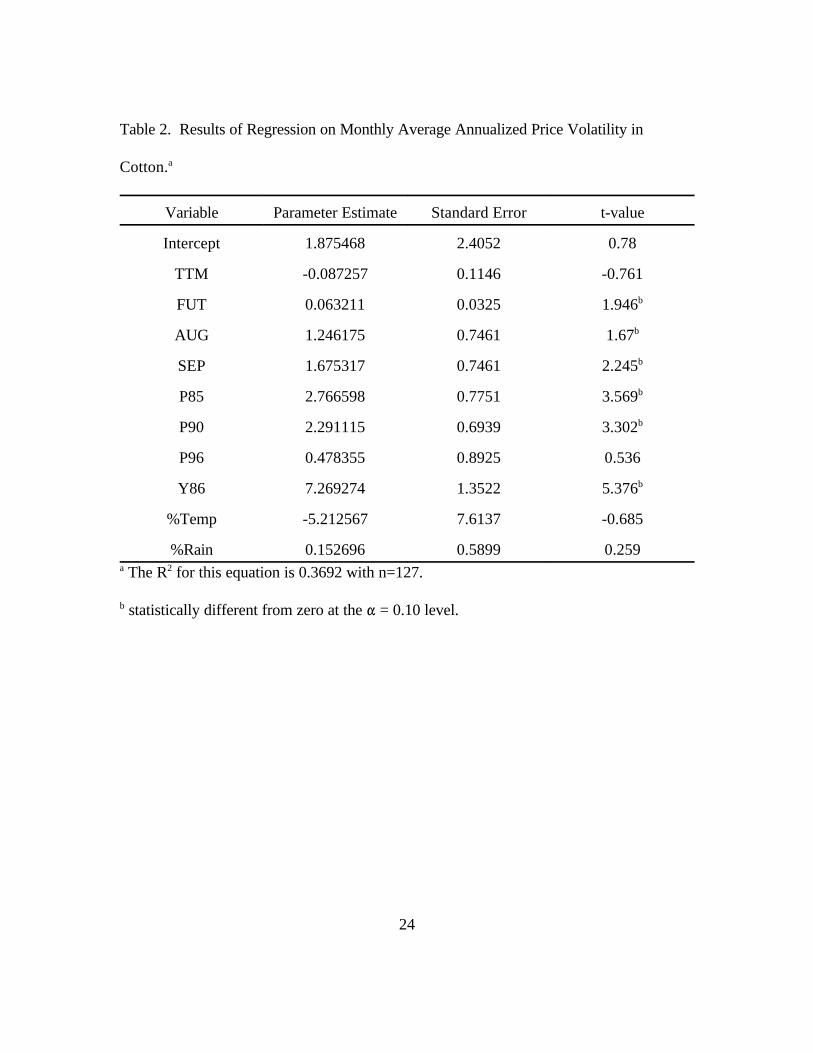
The Durbin-Watson statistic resulting from the initial estimation of Equation 4

showed signs of significant autocorrelation. Equation 4 was thus corrected for

autocorrelation, and Table 2 shows the resulting parameter estimates using the Cochrane-

Orcutt procedure. The model R2 was 0.3692, which indicates that the model only

explained 36.92% of the variation in cotton price volatility. This appears low, but is

consistent with other models of this type in other commodities. It is important to note that

the model is attempting to explain price variability, not price levels, so explanatory power

is expected to be lower.

The sign on the estimate for time-to-maturity (TTM) is consistent with a priori

expectations, but is not statistically significant. This suggests that, after controlling for

other factors, there is no significant time-to-maturity effect. This result is consistent with

prior work in other commodities and suggests that the Samuelson hypothesis is not

tenable when other explanatory factors are considered.

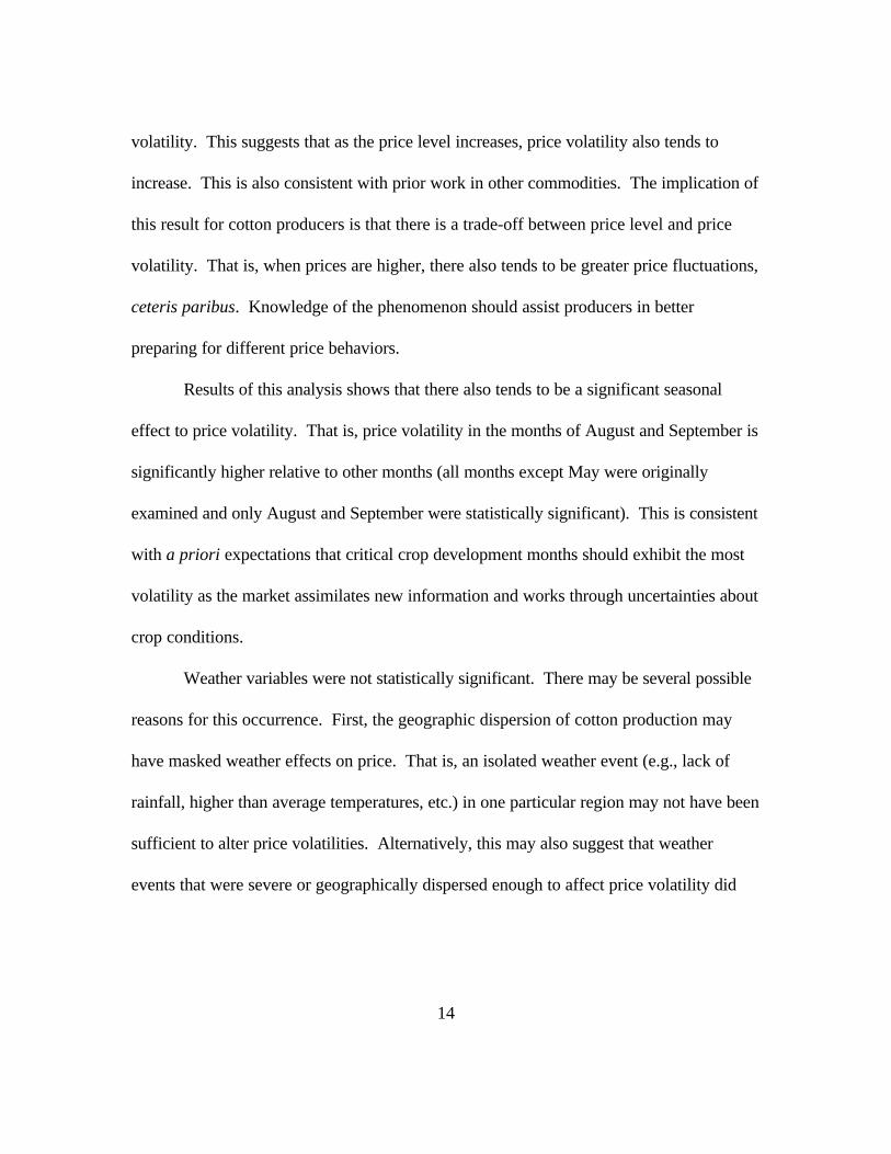
The average monthly futures price is directly and significantly related to price

14

volatility. This suggests that as the price level increases, price volatility also tends to

increase. This is also consistent with prior work in other commodities. The implication of

this result for cotton producers is that there is a trade-off between price level and price

volatility. That is, when prices are higher, there also tends to be greater price fluctuations,

ceteris paribus. Knowledge of the phenomenon should assist producers in better

preparing for different price behaviors.

Results of this analysis shows that there also tends to be a significant seasonal

effect to price volatility. That is, price volatility in the months of August and September is

significantly higher relative to other months (all months except May were originally

examined and only August and September were statistically significant). This is consistent

with a priori expectations that critical crop development months should exhibit the most

volatility as the market assimilates new information and works through uncertainties about

crop conditions.

Weather variables were not statistically significant. There may be several possible

reasons for this occurrence. First, the geographic dispersion of cotton production may

have masked weather effects on price. That is, an isolated weather event (e.g., lack of

rainfall, higher than average temperatures, etc.) in one particular region may not have been

sufficient to alter price volatilities. Alternatively, this may also suggest that weather

events that were severe or geographically dispersed enough to affect price volatility did

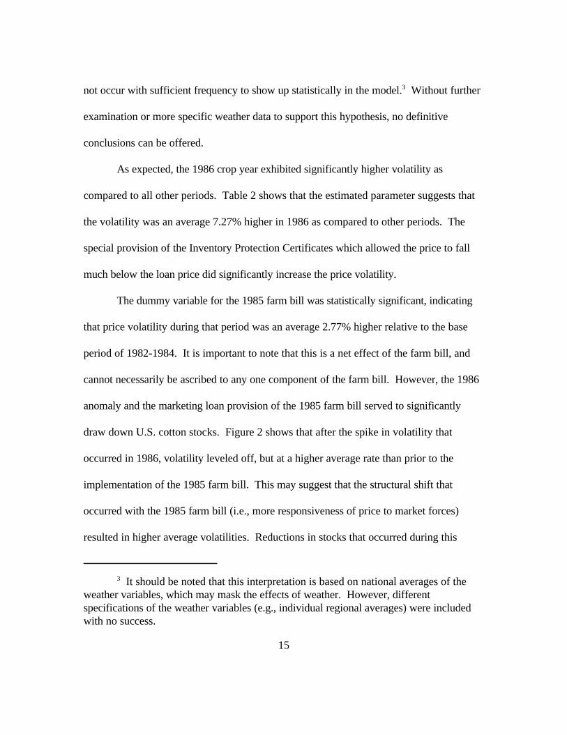
3 It should be noted that this interpretation is based on national averages of theweather variables, which may mask the effects of weather. However, differentspecifications of the weather variables (e.g., individual regional averages) were includedwith no success.

15

not occur with sufficient frequency to show up statistically in the model.3 Without further

examination or more specific weather data to support this hypothesis, no definitive

conclusions can be offered.

As expected, the 1986 crop year exhibited significantly higher volatility as

compared to all other periods. Table 2 shows that the estimated parameter suggests that

the volatility was an average 7.27% higher in 1986 as compared to other periods. The

special provision of the Inventory Protection Certificates which allowed the price to fall

much below the loan price did significantly increase the price volatility.

The dummy variable for the 1985 farm bill was statistically significant, indicating

that price volatility during that period was an average 2.77% higher relative to the base

period of 1982-1984. It is important to note that this is a net effect of the farm bill, and

cannot necessarily be ascribed to any one component of the farm bill. However, the 1986

anomaly and the marketing loan provision of the 1985 farm bill served to significantly

draw down U.S. cotton stocks. Figure 2 shows that after the spike in volatility that

occurred in 1986, volatility leveled off, but at a higher average rate than prior to the

implementation of the 1985 farm bill. This may suggest that the structural shift that

occurred with the 1985 farm bill (i.e., more responsiveness of price to market forces)

resulted in higher average volatilities. Reductions in stocks that occurred during this

16

period (as a result of the policy changes) removed the buffer that likely held volatilities

lower prior to the 1985 farm bill.

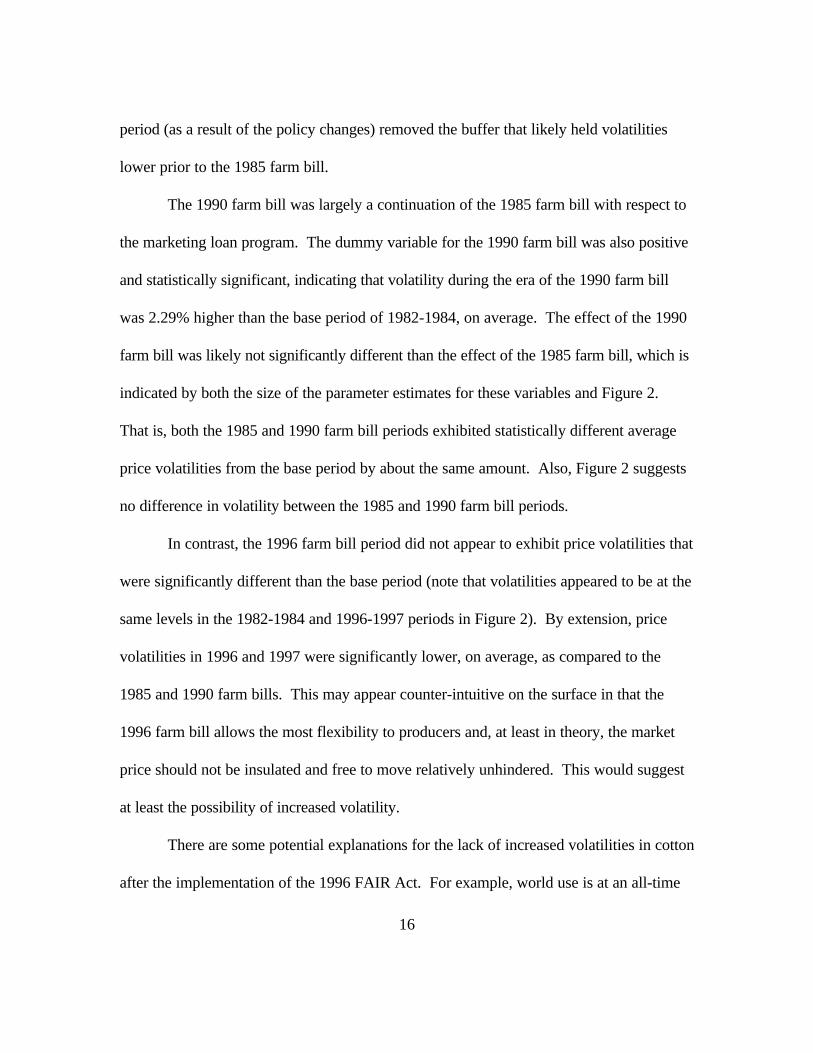
The 1990 farm bill was largely a continuation of the 1985 farm bill with respect to

the marketing loan program. The dummy variable for the 1990 farm bill was also positive

and statistically significant, indicating that volatility during the era of the 1990 farm bill

was 2.29% higher than the base period of 1982-1984, on average. The effect of the 1990

farm bill was likely not significantly different than the effect of the 1985 farm bill, which is

indicated by both the size of the parameter estimates for these variables and Figure 2.

That is, both the 1985 and 1990 farm bill periods exhibited statistically different average

price volatilities from the base period by about the same amount. Also, Figure 2 suggests

no difference in volatility between the 1985 and 1990 farm bill periods.

In contrast, the 1996 farm bill period did not appear to exhibit price volatilities that

were significantly different than the base period (note that volatilities appeared to be at the

same levels in the 1982-1984 and 1996-1997 periods in Figure 2). By extension, price

volatilities in 1996 and 1997 were significantly lower, on average, as compared to the

1985 and 1990 farm bills. This may appear counter-intuitive on the surface in that the

1996 farm bill allows the most flexibility to producers and, at least in theory, the market

price should not be insulated and free to move relatively unhindered. This would suggest

at least the possibility of increased volatility.

There are some potential explanations for the lack of increased volatilities in cotton

after the implementation of the 1996 FAIR Act. For example, world use is at an all-time

17

record level, but is not expected to increase. World production is steady or slightly

increasing. This situation suggests stable world prices. Hence, there has been nothing to

really “move” the market, resulting in lower volatilities. World stocks have been

increasing in recent years, which also tends to have a dampening effect on volatility.

Sudden shocks in either supply or demand may dramatically increase price volatility in the

future. But, at least to date, that has not occurred. Additionally, prices have tended to be

at lower levels in the 1996-1997 period compared to recent years, which may also help

explain lower volatilities.

Conclusions

The results of this analysis provide further evidence that the time-to-maturity effect

is not significant when accounting for other important explanatory variables in futures

price volatility. Although consistent with prior empirical work in other commodities, this

appears to be the first evidence supporting this conclusion in cotton. No time-to-maturity

effect can have implications for traders in that there appears to be no definitive relationship

between time remaining in the contract and volatility. Thus, one cannot predict the size of

price fluctuations based solely on the amount of time left to maturity.

The level of futures prices and seasonality effects also appear to be explanatory

factors that cotton has in common with other commodities. However, weather is not

statistically important. This may result from differences between the production patterns

of cotton and the major grains (particularly corn and soybeans). That is, cotton

production is geographically dispersed, both nationally and globally. This dispersion may

18

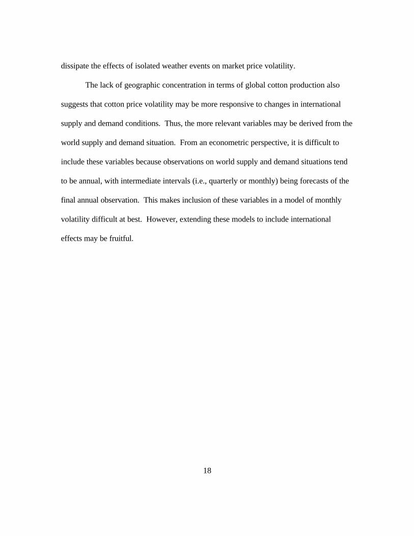
dissipate the effects of isolated weather events on market price volatility.

The lack of geographic concentration in terms of global cotton production also

suggests that cotton price volatility may be more responsive to changes in international

supply and demand conditions. Thus, the more relevant variables may be derived from the

world supply and demand situation. From an econometric perspective, it is difficult to

include these variables because observations on world supply and demand situations tend

to be annual, with intermediate intervals (i.e., quarterly or monthly) being forecasts of the

final annual observation. This makes inclusion of these variables in a model of monthly

volatility difficult at best. However, extending these models to include international

effects may be fruitful.

19

References

Anderson, R. “Some Determinants of the Volatility of Futures Prices.” The Journal of

Futures Markets, 5(1985): 331-348.

Benninga, S., R. Eldor, and I. Zilcha. “Optimal Hedging in the Futures Market Under

Price Uncertainty.” Economics Letters, 13 (1983): 141-145.

Feder, G., R. Just, and A. Schmitz. “Futures Markets and the Theory of the Firm Under

Price Uncertainty.” Quarterly Journal of Economics, 44 (1980): 317-328.

Glade, E., Jr., L. Meyer, and S. MacDonald. “Cotton: Background for 1995 Farm

Legislation.” U.S. Dept. of Ag., Economic Research Service, Washington, DC,

Agricultural Economic Report Number 706, April, 1995.

Glauber, J. and R. Heifner. “Forecasting Futures Price Variability.” Applied Commodity

Price Analysis, Forecasting, and Market Risk Management, Proceedings of the NCR-134

Conference, St. Louis, MO., 1986, pp. 155-165.

Grant, D. “Theory of the Firm with Joint Price and Output Risk and a Forward Market.”

American Journal of Agricultural Economics, 67 (1985): 630.635.

20

Heifner, R. “Hedging Potential in Grain Storage and Livestock Feeding.” Agricultural

Economics Report 238, U.S. Department of Agriculture, Washington, DC, 1973.

Heifner, R. “Can Option Forecast Crop Price Volatility over the Growing Season?”

Selected Paper presented at the American Agricultural Economics Association Annual

Meeting, Toronto, Canada, July 27-30, 1997.

Hennesey, D. and T. Wahl. “The Effects of Decision Making on Futures Price Volatility.”

American Journal of Agricultural Economics, 78(1996): 591-603.

Hull, J. Options, Futures, and Other Derivatives. Third Edition, Prentice Hall Publishers,

Upper Saddle River, NJ, 1997.

Kahl, K. “Determination of the Recommended Hedging Ratio.” American Journal of

Agricultural Economics, 65 (1983): 603-305.

Kenyon, D., K. Kling, J. Jordan, W. Seale, and N. McCabe. “Factors Affecting

Agricultural Futures Price Variance.” The Journal of Futures Markets, 7(1987): 73-91.

Lapan, H. and G. Moschini. “Futures Hedging Under Price, Basis, and Production Risk.”

American Journal of Agricultural Economics, 76 (1994): 465-477.

21

Lence, S. and D. Hayes. “The Empirical Minimum-Variance Hedge.” American Journal of

Agricultural Economics, 76(1994): 94-104.

McKinnon, R. “Futures Markets, Buffer Stocks, and Income Stability for Primary

Producers.” Journal of Political Economy, 75 (1967): 844-861.

Milonas, N. “Price Variability and the Maturity Effect in Futures Markets.” The Journal of

Futures Markets, 6(1986): 443-460.

Moschini, G. and H. Lapan. “The Hedging Role of Options and Futures Under Joint Price,

Basis, and Production Risk.” International Economics Review, 36 (1995): 1025-1049.

NASS. “Crop Progress Reports.” U.S. Dept. of Ag., National Agricultural Statistics

Service, Washington, DC, Various Issues.

Ray, D., J. Richardson, D. De La Torre Ugarte, K. Tiller. “Estimating Price Variability in

Agriculture: Implications for Decision-Makers.” Invited Paper presented at the Southern

Agricultural Economics Association Annual Meeting, Little Rock, AR, February 1-4,

1998.

22

Sakong, Y., D. Hayes, and A. Hallam. “Hedging Production Risk with Options.”

American Journal of Agricultural Economics, 75(1993): 408-415.

Samuelson, P. “Proof that Properly Anticipated Prices Fluctuate Randomly.” Industrial

Management Review, 6(1965): 41-49.

Streeter, D. and W. Tomek. “Variability in Soybean Futures Prices: An Integrated

Framework.” The Journal of Futures Markets, 12(1992): 705-728.

23

Table 1. Percentage Annualized Volatilities in the December Futures Contract for Cotton,

1982-1997.

May Jun Jul Aug Sep Oct Nov Dec

1982 4.36 7.92 7.48 7.63 6.62 5.20 5.56 4.60

1983 6.84 9.34 8.60 8.30 8.32 5.99 7.40 5.16

1984 6.31 6.14 6.28 6.43 4.15 7.26 7.56 2.20

1985 5.73 4.69 6.35 4.81 3.21 4.59 4.89 3.71

1986 10.56 8.27 15.10 14.28 24.41 16.04 15.02 13.32

1987 9.96 13.47 7.61 9.71 11.51 10.50 13.11 12.04

1988 11.52 15.51 9.43 11.34 12.04 11.69 9.94 9.14

1989 5.03 10.5 6.39 8.41 9.35 6.72 8.33 12.39

1990 4.46 5.31 8.71 7.93 7.40 5.71 7.77 1.95

1991 8.61 8.94 8.26 9.61 8.73 7.48 11.88 7.73

1992 9.46 8.58 7.29 11.50 9.73 9.56 11.39 4.15

1993 4.92 4.79 10.22 10.12 8.82 6.82 8.27 8.26

1994 4.74 7.27 10.66 9.80 7.44 8.08 8.45 16.14

1995 10.59 10.36 10.43 12.46 15.77 12.01 7.74 6.86

1996 7.98 7.06 6.77 10.81 10.27 8.54 7.01 7.44

1997 2.76 5.49 5.93 4.69 6.41 3.99 5.96 10.53

Avg. 7.11 8.35 8.47 9.24 9.63 8.14 8.77 7.85

24

Table 2. Results of Regression on Monthly Average Annualized Price Volatility in

Cotton.a

Variable Parameter Estimate Standard Error t-value

Intercept 1.875468 2.4052 0.78

TTM -0.087257 0.1146 -0.761

FUT 0.063211 0.0325 1.946b

AUG 1.246175 0.7461 1.67b

SEP 1.675317 0.7461 2.245b

P85 2.766598 0.7751 3.569b

P90 2.291115 0.6939 3.302b

P96 0.478355 0.8925 0.536

Y86 7.269274 1.3522 5.376b

%Temp -5.212567 7.6137 -0.685

%Rain 0.152696 0.5899 0.259a The R2 for this equation is 0.3692 with n=127.

b statistically different from zero at the " = 0.10 level.

25

6.00

6.50

7.00

7.50

8.00

8.50

9.00

9.50

10.00

May Jun Jul Aug Sep Oct Nov Dec

Month

% V

olat

ility

Figure 1. Monthly Average Price Volatility, December Contract, 1982-1997.

26

0

5

10

15

20

25

30

Year

1983

1984

1986

1987

1988

1990

1991

1992

1994

1995

1997

Ann

ualiz

ed V

olat

ility

in %

Figure 2. Annualized Monthly Price Volatilities by Month, 1982-1997.