
The impact of institutional volatility on financial volatility in transition economies: a GARCH...
63
BOFIT Discussion Papers 6 • 2014 Christopher A. Hartwell The impact of institutional volatility on financial volatility in transition economies: a GARCH family approach Bank of Finland, BOFIT Institute for Economies in Transition
-
Upload
morningstar -
Category
Documents
-
view
0 -
download
0
Transcript of The impact of institutional volatility on financial volatility in transition economies: a GARCH...

BOFIT Discussion Papers 6 • 2014
Christopher A. Hartwell
The impact of institutional volatility on financial volatility in transition economies: a GARCH family approach
Bank of Finland, BOFIT Institute for Economies in Transition

BOFIT Discussion Papers Editor-in-Chief Laura Solanko BOFIT Discussion Papers 6/2014 13.2.2014 Christopher A. Hartwell: The impact of institutional volatility on financial volatility in transition economies: a GARCH family approach ISBN 978-952-6699-72-1 ISSN 1456-5889 (online) This paper can be downloaded without charge from http://www.bof.fi/bofit. Suomen Pankki Helsinki 2014

BOFIT- Institute for Economies in Transition Bank of Finland
BOFIT Discussion Papers 6/ 2014
3
Contents
Abstract .................................................................................................................................. 4
1 Introduction ................................................................................................................... 5
2 Literature review: institutions, volatility and the financial sector ................................. 7
3 Methodology and empirical model .............................................................................. 10
4 Data and diagnostics .................................................................................................... 14
5 Results ......................................................................................................................... 23
6 Conclusions ................................................................................................................. 28
Tables and figures ................................................................................................................ 30
References ........................................................................................................................... 55
Christopher A. Hartwell The impact of institutional volatility on financial volatility in transition economies: a GARCH family approach
4
Christopher A. Hartwell
The impact of institutional volatility on financial volatility in transition economies: a GARCH family approach
Abstract The volatility of financial markets has been a relevant topic for transition economies, as the
countries of Central and Eastern Europe and the former Soviet Union have seemingly en-
dured high levels of volatility in their financial sectors during the transition process. But
what have been the determinants of this financial volatility? This paper posits that institu-
tional changes, and in particular the volatility of various crucial institutions, have been the
major causes of financial volatility in transition. Examining 20 transition economies over
various time-frames within the period 1993–2012, this paper applies the GARCH family of
models to examine financial volatility as a function of institutional volatility. The results
from the EGARCH and TGARCH modelling supports the thesis that more advanced and
more stable institutions help to dampen financial sector volatility at their levels, while in-
stitutional volatility feeds through directly to financial sector volatility in transition.
Keywords: institutions, financial sector, volatility, transition, GARCH, EGARCH,
TGARCH
JEL Codes: G20, O43, P30
Christopher A. Hartwell, PhD. Head of Markets and Institutions Research Institute for Emerging Market Studies (IEMS), Moscow School of Management, SKOLKOVO, Novaya ul. 100, Skolkovo village, Odintsovsky District, Moscow Region, 143025, Russia. E-mail: [email protected]; [email protected]. Phone: +7 916 777 1260 (t), +7 495 994 46 68 (f) Acknowledgements I would like to thank the Bank of Finland Institute for Economies in Transition (BOFIT) for supporting this research and providing excellent data access, and especially Laura Solanko for her encouragement and com-ments. I also thank Mikhail Volkov for excellent and persistent research assistance throughout the creation of this paper, as well as participants at the ‘Economic Challenges in Enlarged Europe’ Conference in Tallinn, Estonia (June 16–18, 2013) for their comments, especially Karsten Staehr, Josef Brada and Anna Zamojska. Additional thanks go to participants at the ACES poster session during the ASSA Conference 2014, including Ali M. Kutan and Joseph Brada. All errors remain my own.

BOFIT- Institute for Economies in Transition Bank of Finland
BOFIT Discussion Papers 6/ 2014
5
1 Introduction Owing to the severity of the global financial crisis and the apparent increased incidence of
financial crises over the past twenty years, the examination of financial volatility and its
determinants has become a fruitful and important topic for economists in recent years. Part
of this interest is the fact that financial assets and instruments apparently have a much
higher level of volatility than ‘real’ output, such as consumption, growth, and savings; the
more relevant fact, however, is that persistent financial volatility can feed through to and
damage the real economy. As Daly (2011:46) noted, these effects, especially if they appear
unrelated to economic fundamentals, “may lead to an erosion of confidence in capital mar-
kets and a reduced flow of capital into equity markets.” Thus, ascertaining the determi-
nants of financial volatility would appear to be a first step towards reducing the possible
effects of this volatility on the real economy.
The volatility of financial markets has similarly been a relevant topic for transition
economies as well, as the countries of Central and Eastern Europe (CEE) and the former
Soviet Union (FSU) have seemingly endured higher levels of volatility in their financial
sectors during the transition process. With financial crises ranging from region-wide
breakdowns, such as Russia in 1998−99 and the global financial and Eurozone crises from
2007 to the present, to country-specific crises such as Latvia in the mid−1990s and Slova-
kia in the late 1990s, the countries transitioning from communism to capitalism appear to
have felt first-hand the damaging consequences of financial volatility.
However, while the determinants of financial sector volatility have been studied in
a developing country context, there has been a notable lack of focus exclusively on transi-
tion economies. Indeed, much of the transition literature has treated the rise of financial
volatility as part of the broader transition process, an inevitable by-product of the learning
curve of financial sector institutions and the volatile macroeconomic environment that the
financial sector faces in transition. But has this really been the case? What are the drivers
of financial volatility that appear to plague even late-stage transition economies?
An obvious culprit for the source of this volatility would appear to be the financial
liberalization that accompanied transition. Financial liberalization, including the freeing of
interest rates, allowance of private banks (internal liberalization) and removal of capital
controls (external liberalization) has been part and parcel of the transition to capitalism. An
extensive literature links financial sector liberalization in transition with expansion of

Christopher A. Hartwell The impact of institutional volatility on financial volatility in transition economies: a GARCH family approach
6
credit to the private sector (Cottarelli, Dell’Ariccia and Vladkova-Hollar (2005)), devel-
opment of sound banks (Fries and Taci (2002)), growth in firm sales and use of debt for
financing (Giannetti and Ongena (2009)) and, teamed with governmental fiscal and mone-
tary responsibility (Berglof and Bolton (2002)), sustained economic growth (Akimov, Wi-
jeweerab and Dollery (2009)). But while there may be some theoretical conjecture on the
link between liberalization and extreme volatility (as in Stiglitz (2002), where he argues
the premature exposure of immature financial institutions to world markets will bring more
harm than good), there has been little formal work done linking financial liberalization
with volatility in transition economies. This does not mean that the volatility does not ex-
ist: as Buiter (2003) and Egert and Koubaa (2004) point out, “in general, equity markets in
Central and Eastern Europe are high yield, volatile markets” (Buiter (2003: 132)). It does
mean that the modelling of volatility and financial liberalization in transition is at a very
early stage.
Perhaps a deeper explanation, however, for the uptick in financial volatility in
transition relates to the very reason for transition, and that is the change of institutions from
communist-era to capitalist institutions. Given that changes in financial sector institutions
in transition occur in tandem with broader institutional changes throughout an economy, it
is not unreasonable to assume that the broader institutional environment will both influence
financial sector development and influence the incidence of volatility. Here, too, there is a
noticeable gap in the literature regarding the interactions of economic institutions and fi-
nancial institutions; Coricelli and Maurel (2011) is one of the few papers to model the in-
terplay of financial institutions and other market-supporting institutions, but they shy away
from the concept of volatility. Other studies that do delve into volatility in transition like-
wise miss the institutional aspect, limited to an examination of macroeconomic variables
and their effect on volatility (see, for example, Hsing and Hsieh (2012)).
The purpose of this paper is, thus, to examine several interrelated questions re-
garding the nature of institutions and financial volatility in transition:
• Did economic and political institutions, specifically property rights and de-
mocratic accountability, have a discernible effect on financial sector volatility during the transition period?
• Do other macroeconomic variables found to already have an impact in the lit-erature on volatility (such as growth of M2/GDP, as in Hsing and Hsieh (2012)) have more or less of an effect in the presence of market-supporting institutions?

BOFIT- Institute for Economies in Transition Bank of Finland
BOFIT Discussion Papers 6/ 2014
7
• Did the volatility of these institutions and their changes during the transition period affect financial markets? Put simply, did institutional volatility feed through to financial volatility?
This paper makes a novel contribution to the literature on financial sector institutions and
transition economics in three ways. First, it examines the institutional influence on finan-
cial sector volatility exclusively for transition economies, an issue that has been little ex-
plored except in the context of the transition process itself. Secondly, this paper uses
monthly institutional data from transition economies, a difficult but appropriate choice in
an environment in flux and where institutional change is precisely the goal of transition.
Thirdly, given this higher-frequency data, we explore the impact of institutional volatility
on financial sector volatility through the use of the ARCH/GARCH family of models. This
paper would be the first, to my knowledge, to explicitly model financial volatility in transi-
tion countries exclusively as a function of institutional volatility.
The rest of the paper proceeds as follows. Section II discusses the literature be-
hind institutional volatility, while Section III describes the empirical model used in this
paper to investigate these questions. Section IV discusses the data and diagnostics utilized,
while Section V presents estimation results on the series of GARCH-family models util-
ized. Section VI concludes with implications and future avenues for research.
2 Literature review: institutions, volatility and the financial sector
A voluminous literature exists in finance and economics on the determinants of stock mar-
ket volatility, with these determinants loosely grouped into three separate areas:
• The intrinsic or actualized attributes of stock markets that make them suscep-
tible, such as systematic risk, size or capitalization (Bekaert and Harvey (1997)), turnover (Andersen (1996)), leverage (Christie (1982)) and other at-tributes of a particular stock exchange (Gabaix et al. (2006));
• Domestic and international macroeconomic factors and policies (Schwert (1989)), including growth (Beltratti and Morana (2006)), inflation (Flannery and Protopapadakis (2002)), credit (Gourinchas, Valdes and Landerretche (2001)), overall macroeconomic health (Errunza and Hogan (1998)) and other business cycle factors exogenous to the stock exchange but not necessarily to the specific country (Bollerslev and Zhou (2006)); and

Christopher A. Hartwell The impact of institutional volatility on financial volatility in transition economies: a GARCH family approach
8
• Behaviour and performance of other stock markets (King and Wadhwani (1990), Forbes and Rigobon (2002), Beirne et al. (2009) and literally hun-dreds of other papers), as a method of importing either stability or volatility ex-ogenous to both specific stock exchanges and specific countries.
However, while the first area of research somewhat concerns the workings of a stock ex-
change as an institution in and of itself (see Demirgüç-Kunt and Levine (1996)), there has
been little work done on the interplay between institutions outside of the stock market and
performance within the exchange. This omission is somewhat puzzling, but can be ex-
plained by the fact that the impact of institutions on economic growth and other metrics of
economic success is still a young (if growing) field, characterized by both high-level ar-
guments about the relative impact of institutions (Sachs (2003), Rodrik, Subramanian and
Trebb (2004), Acemoglu and Johnson (2005)) and, more recently, highly detailed research
about the impact of specific institutions (Hartwell (2013)). By contrast, the relationship
between institutions and the financial sector has been conducted mainly at the higher level,
focusing on overviews that answer the question if institutions influence financial sector de-
velopment and activity. The overwhelming consensus is “of course”, with work such as
Claessens and Laeven (2003) finding that property rights improve asset allocation in the
financial sector, which then in turn leads to positive effects on growth in sectoral value.
Andrianaivo and Yartey (2009) reinforce this result, finding that one important facet of
property rights, creditor protection, is a strong and highly significant factor in financial
sector development in Africa. Other work from Beck and Levine (2008) concludes that le-
gal origins can account for differences in property rights regimes and thus the development
of a country’s financial sector, while Demirgüç-Kunt and Levine (1996) find that countries
with well-developed institutional systems tend to have large and liquid stock markets and
Durham (2002) notes that rule of law and institutions more broadly support financial de-
velopment. Chinn and Ito (2006) also find that ‘general’ institutional quality indicators,
such as rule of law and bureaucratic quality, support successful financial sector develop-
ment more than financial sector-specific institutions (such as transparency of accounting
procedures).
Given the large amount of evidence linking institutional quality to financial sector
development and, in many cases, performance, it stands to reason that institutional changes
would also translate through to financial sector outcomes. But as noted above, in regards to
the financial sector, the issue of the effects of institutional volatility or instability has been

BOFIT- Institute for Economies in Transition Bank of Finland
BOFIT Discussion Papers 6/ 2014
9
relatively less explored in the literature. Part of this can be attributable to the reality that
institutional volatility is rarely observed, given that institutional changes tend to take place
over a long period of time (as opposed to financial sector movements, which are very high-
frequency) and may be unrecognizable to outside observers; moreover, while theories re-
garding institutions are relatively well-developed in both economics (North (1971)) and
political science literature (see especially Levitsky and Murillo (2009)), quantification of
institutions is still an area that is in its infancy (see Moers (1999) and Voigt (2013) for a
lively debate on how to even measure institutions). Given this basic fact of slow-paced in-
stitutional change (and the difficulty of quantifying it), researchers interested in volatility
have gravitated more towards examining ‘policy uncertainty’ as a determinant of financial
sector outcomes. A somewhat first-order solution to a second-order issue (after all, policies
are the inputs that can shape institutions and their development, either explicitly or implic-
itly), the policy uncertainty literature has laid a theoretical groundwork for the effects of
institutional volatility, with papers such as Rodrik (1991), Aizenman and Marion (1993)
and Baker, Bloom, and Davis (2013) focusing on the feed-through of instability to the real
economy via expectations and investment decisions.
This does not mean that explicit modelling of institutional volatility has been en-
tirely neglected, as much of the work that has been done in this area has been focused on
quantification of the impact of institutional instability on economic growth, rather than on
financial sector outcomes. Brunetti and Weder (1998) focus on changes in national-level
institutions, including constitutional changes and probability of institutional shifts (based
on survey data), finding that constitutional changes (i.e. political volatility) are negatively
correlated with growth. In a similar vein, Svensson (1998) examines political institutional
volatility, modelling the effect of political institutions on economic ones (in this case,
property rights). His results point to a negative effect on investment, with the probability of
an imminent political change (derived from a probit model) harming property rights forma-
tion, which then in turn feeds through to investment decisions (Yang (2011) also finds that
normal democratic processes tend to increase macroeconomic instability). Berggren, Bergh
and Bjornskov (2011) take this examination even further to model the effects of institu-
tional ‘instability’ on growth, using coefficients of variation from a set of institutional
measures (constructed by principal components analysis) to proxy for instability over a
five-year period. Using a GLS estimator with fixed effects and controlling for other macro-
economic influences, their results are ‘context dependent’: in particular, they find that in-

Christopher A. Hartwell The impact of institutional volatility on financial volatility in transition economies: a GARCH family approach
10
stability in legal and policy institutions in rich countries actually contributes significantly
to higher growth rates, while instability of social institutions is a drag on growth across all
countries.
Beyond the linkages between growth and institutional volatility, the economics
research tends to thin out, with other disciplines only taking up the slack marginally. For
example, Chung and Beamish (2005) examine the dynamic nature of institutions in the
context of multinational decisions in emerging economies, finding that firms that are either
wholly-owned subsidiaries or majority-domestic joint ventures weather periods of institu-
tional volatility better than mostly ‘foreign’ firms. Other researchers have come at the issue
of institutional volatility from either a law or political science perspective; Gallo and
Alston (2008), for example, place the difficulties in Argentina’s banking system since 1949
as a function of the breakdown of judicial independence and purge of 80% of the Supreme
Court justices in 1947. Similarly, Stern et al. (2002) come closer to the issue of financial
sector performance and institutional volatility, but their focus is less on the impact of insti-
tutional volatility on the financial sector as on the second-order impact on governmental
crisis management in the Baltic countries. More recent work from Bialkowski, Gottschalk
and Wisniewski (2008) and Boutchkova et al. (2012) also touches on the financial sector in
an examination of elections and their financial impact, concluding that the variance in a
country’s major index return doubles during an election week. However, the idea that sus-
tained or unexpected institutional volatility (after all, elections are planned months, if not
centuries, in advance) can have immediate effects on financial performance throughout the
economy has remained unexplored.
3 Methodology and empirical model The GARCH family and institutions This paper attempts to rectify the above-mentioned omission through the application of
some innovative econometric tools. While these prior papers may have looked at institu-
tional volatility writ large, they have shied away from using one of the most powerful tools
for exploring conditional variance: the autoregressive conditionally heteroskedastic
(ARCH) family of models. A major contribution of this current paper is to apply the
ARCH family to institutional volatility in specifically transition economies. While ARCH

BOFIT- Institute for Economies in Transition Bank of Finland
BOFIT Discussion Papers 6/ 2014
11
models have been utilized to investigate the effects of financial volatility in a large and
well-established literature (Engle (1982), Hayo and Kutan (2005) and Wu and Shea (2011)
are but a few examples), ARCH modelling in institutional economics is relatively unheard
of.
Much of this omission of ARCH applications is due to the nature of the beast be-
ing examined. ARCH models are typically used with high-frequency data, and institutions
are the complete antithesis of data such as daily stock market returns. Indeed, the persistent
nature of institutions is one of the key things that defines them as ‘institutions’: their time-
invariant nature, characterized by semi-permanence, is perhaps the most important distin-
guishing feature of institutions versus policies and other attributes of the economy. This
problem has bedevilled quantitative institutional economics, as institutional changes can
occur either over a long period of time through very gradual evolution (as in the case of
religious dogma) or in a sudden structural break; in the first instance, quantification of in-
stitutions would show only the most minute changes (if any) over a long period, while in
the second, large changes may be missed in highly aggregated data.
However, ARCH models also have positives that recommend them to the applica-
tion of institutional changes, especially in the context of transition economies. In the first
instance, they can deal with the specific attributes of institutions that may skew normal
econometric estimation: institutional shocks can display a high degree of persistence (if not
an outright structural break) due to their slow-moving and slow-changing nature, and the
volatility of institutional change is not constant over time. More importantly, and address-
ing the issue of permanence, institutions in transition economies are fundamentally differ-
ent to the semi-permanent institutions normally examined in the literature. Indeed, the tran-
sition from communism to capitalism is precisely about the accelerated evolution of insti-
tutions, the replacement of one set of institutions with another. These transition processes
are almost entirely designed to follow in reality what an ARCH model is designed to cap-
ture econometrically: periods of large and volatile movements, followed by periods of
‘normalcy’, only to be followed again by high volatility, either endogenously or exoge-
nously generated. Given this conditionally heteroskedastic nature of institutions and transi-
tion itself, ARCH models may help to capture this non-constant variance.
Thus, in regards to both financial volatility and institutional volatility, the ARCH
family of models, as standard tools for modelling volatility, have value added that may not
be present in other estimators. For example, while GMM estimators are equipped to handle

Christopher A. Hartwell The impact of institutional volatility on financial volatility in transition economies: a GARCH family approach
12
conditional heteroskedasticity, as Fleming (1998) notes, time-series volatility data have a
high degree of serial correlation that may generate spurious results in a GMM framework.
In this data-set especially (and as noted below), there is high persistence of volatility,
meaning longer lags of variables would be needed as valid instruments; as Tauchen (1986:
397) notes, however, the bias of GMM rises as more instruments based on deeper lags of
variables are introduced, leading to estimates concentrating “around biased values [while]
confidence intervals become misleading.” Finally, diagnostic tests using a ‘system-GMM’
approach with this sizeable dataset inevitably resulted in an over-proliferation of instru-
ments even after collapsing instruments and restricting lags, a problem that Roodman
(2009) has noted can lead to imprecise estimates of the optimal weighting matrix.
Having settled on the relative merits of the ARCH family, for this examination,
the next step is choosing the appropriate estimator from the alphabet soup of ARCH mod-
els, which is of course conditioned by the dataset. While Lunde and Hansen (2005) tout the
predictive power of a simple GARCH (1,1) model versus other challengers, there are ef-
fects in this data and related to the idiosyncrasies of institutions in general that may need
additional modelling power. Choosing an appropriate model becomes more difficult as, to
date, only a few outstanding papers have been produced in the past decade attempting to
apply ARCH models to institutional variables: these include Asteriou and Price (2001),
Henisz (2004), Jayasuriya (2005), Klomp and De Haan (2009)1 and the spiritual father of
this current paper, Campos and Karanasos (2008). Asteriou and Price (2001) use both a
GARCH and GARCH in means (GARCH-M) model to test the effects of political uncer-
tainty on the conditional variance of GDP growth in the United Kingdom. Constructing a
principal components measure of political instability from various indicators including
strikes and terrorism, they find that political instability has a highly negative, significant
and persistent effect on GDP growth. Similarly, in order to examine the effects of political
instability on growth in Argentina, Campos and Karanasos (2008) apply a Power-ARCH
(PARCH) model, as first introduced by Ding, Granger and Engle (1993); in their words,
the PARCH model “increases the flexibility of the conditional variance specification by
allowing the data to determine the power of growth for which the predictable structure in
the volatility pattern is the strongest” (Campos and Karanasos (2008:136)). Their results
1 Klomp and De Haan (2009) utilize GARCH (1,1) modelling in order to isolate their political uncertainty variables, but otherwise include these variables in a standard GMM and mean group series of panel data es-timations.

BOFIT- Institute for Economies in Transition Bank of Finland
BOFIT Discussion Papers 6/ 2014
13
also find that both formal (government changes) and informal (assassinations) political
volatility affected growth in Argentina over 1896–2000, with informal volatility having a
greater short-run and direct effect.
In regards to this panel dataset, theoretically, either the exponential generalized
autoregressive conditional heteroskedasticity (EGARCH) model of Nelson (1991), the
threshold GARCH (TGARCH) model of Zakoian (1994), or, as in Campos and Karanasos
(2008), one of the power-ARCH (PARCH or APARCH) models should be the preferred
estimator. This narrowing down of choices is due to the fact that institutional shocks in
transition should exhibit highly asymmetric effects that would not be captured in a simple
GARCH specification: negative institutional shocks in an environment in flux (and where
the end goal is by no means assured) should impact financial volatility much more than a
positive shock (which may be reversed in the next election). Indeed, it can be theorized
that institutional volatility would have a similar effect to bad news, with ‘bad’ institutional
changes having much ‘worse’ effects on volatility (Engle and Ng (1993)), but in a much
more persistent and deeper manner than mere bad news. Given that the EGARCH model
has been used precisely to model this asymmetric response (Braun, Nelson, and Sunier
(1995); Koutmos and Booth (1995); Malik 2011; Andraz and Norte (2013)), it is the front-
runner for inclusion here. Such an EGARCH model would follow the form:
(1) 𝑦𝑖𝑡 = 𝜇𝑖𝑡 + 𝜖𝑡
(2) 𝜇𝑖𝑡 = 𝛼 + 𝛽1𝐼𝑁𝑆𝑇𝑡−1 + 𝛽2𝑀𝐴𝐶𝑅𝑂𝑡−1 + ∑ 𝜋𝜀𝑡−𝑗
𝑛𝑗=𝑖
(3) 𝜀𝑡 = �ℎ𝑡 𝑣𝑡
(4) log(ℎ𝑡) = 𝜔 + ∑ 𝜁𝑖 log�ℎ𝑡−𝑖� + ∑ �𝑛𝑗 �𝑣𝑡−𝑗� + 𝑘𝑗 �𝑣𝑡−𝑗�� + 𝜆𝑃𝑟𝑜𝑝𝑅𝑖𝑔ℎ𝑡𝑠𝑡−1 +𝑞
𝑗=𝑖𝑝𝑖=1
𝜌𝐷𝑒𝑚𝑜𝑐𝑟𝑎𝑐𝑦𝑡−1
where Equation 1 is the whole panel EGARCH model, Equation 2 is the mean equation
and Equations 3 and 4 model the conditional variance as a function of institutional volatil-
ity.2
2 As noted throughout this paper, the approach taken is a panel-GARCH model, due mainly to the research question: did institutional volatility across transition economies affect financial volatility? As Cermeno and Grier (2006) note, “to study the determinants and real effects of uncertainty in the developing world, we need a panel GARCH model”, based on the relative paucity of observations per country and the heightened effects

Christopher A. Hartwell The impact of institutional volatility on financial volatility in transition economies: a GARCH family approach
14
Moreover, the EGARCH κ measure captures the ‘leverage effect’ (Jayasuriya
2005) of institutional volatility, or the idea that negative institutional shocks have a greater
(negative) effect on financial volatility than positive shocks of the same magnitude would.
As Jayasuria (2005) correctly notes, we should thus see the leverage effect be negative in
the conditional variance equation. In contrast to the EGARCH model, the TGARCH speci-
fication of Zakoian (1994) models the conditional variance as a function of the standard
deviation, but it too allows for asymmetric effects of the institutional volatility indicators.
Given the similarity in the treatment of volatility shocks, both EGARCH and TGARCH
models will be attempted below, with post-estimation statistics such as the Akaike infor-
mation criterion (AIC) and the Bayesian information criterion (BIC) used to determine
which approach models the conditional volatility more effectively.
4 Data and diagnostics The Y variable in equation (1) above is financial volatility, which is proxied by two sepa-
rate measures. The first (as is standard in the literature, starting with Merton (1980) and
Perry(1982)), is realized volatility: that is, the volatility of the entire stock market index
returns, as measured by the log sum of squared daily returns, aggregated monthly:
(5) 𝜎2 = log (∑ 𝑟__𝑖𝑡
2𝑁𝑡𝑡=1 )
In equation 5, r is defined as the log difference of the returns in the stock market index of
country i between day t and day t-1, a common formulation in the finance literature to
measure volatility (see Brailsford and Faff (1996), for example, and especially Andersen
and Bollerslev (1998) for a discussion of its suitability).3 This indicator of volatility has the
benefit of long histories in the transition economies (in some cases, such as the Czech Re-
public, 223 separate monthly observations are available) but is unfortunately not available
for all of the countries of Central/Eastern Europe and the former Soviet Union (a complete
that are anticipated in an emerging or transition framework. And while country studies may be developed from this data (noting the relatively shorter data series), the purpose of this paper is to take a broader look at the influence of institutions, and thus the panel structure was retained. It is, of course, possible to examine each country separately (which indeed was done in post-estimation inspection), but that is beyond the scope of this paper. 3 Taking the log of this series is crucial for smoothing the admittedly ‘noisy’ data in the GARCH specifica-tions used later, and also follows a similar approach to Paye (2012), although Paye uses the log of excess returns rather than actual returns.

BOFIT- Institute for Economies in Transition Bank of Finland
BOFIT Discussion Papers 6/ 2014
15
description of the data is shown in Table 1). Moreover, as noted above, there is also a
chance that we are somewhat limiting ourselves in examining this metric of volatility, as a
country must attain a certain level of financial sector development to even have an equity
exchange. However, we believe that, given the wide dispersion of country development
and transition levels (especially at the moment that the various stock exchanges were cre-
ated), the inclusion of stock market volatility as a proxy for overall financial volatility will
still yield fruitful results.
Additional measures of financial volatility will also be utilized for robustness
tests, including the log of absolute returns (as suggested by Ding, Granger, and Engle
(1993)), the log of squared percentage changes (Rogers and Siklos (2003)), and, finally,
the interest rate spread, defined as the difference between the (average) lending rate and
deposit rate in a country for that month. This last measure, unlike stock market returns, is
more of an indirect proxy for volatility, in that it captures ex post facto volatility rather than
direct volatility; as has been empirically noted (see Agenor, Aizenman, and Hoffmaister
(1998)), financial volatility can drive interest rate spreads higher, providing an after-the-
fact picture of a market in turmoil. As noted by Kliesen, Owyang, and Vermann (2012),
high interest rate spreads can also indicate financial sector risk perceptions, which would
also be an important component of financial sector volatility.4
The most important part of this examination, where this paper breaks new ground,
concerns the INST variable shown in Equation 4. At this point, we run into the familiar
debate in institutional economics of subjective versus objective indicators (see Moers
(1999) and Voigt (2013) for a good explanation of both sides’ arguments): succinctly put,
subjective indicators may indicate bias (as they are based on subjective ratings), while ob-
jective indicators may capture much more than the effect under examination, due to their
broad nature. To satisfy both camps, and present a full series of sensitivity and robustness
checks, we approach the quantification of institutional change through utilization of both
subjective and, as a robustness test, objective indicators.
In the aggregate, the institutional variable will be a vector of institutions, both
economic and political, found to be correlated with economic outcomes in transition
economies (see Hartwell (2013) for an extensive treatment of institutional influence in
transition). In terms of economic institutions, property rights, in particular, have been
4 Additionally, other indicators for financial volatility are utilized for sensitivity analyses below.

Christopher A. Hartwell The impact of institutional volatility on financial volatility in transition economies: a GARCH family approach
16
found to have a great impact on financial sector development in transition economies, as
well as being associated strongly with broader successful transition dynamics (Hartwell
2013) and economic growth (Torstensson (1994), Acemoglu and Johnson (2005), Asoni
(2008) and many others). The reason for this association between property rights and fi-
nancial sector development is clear: more secure property rights, in addition to providing
the basis for greater savings (and thus lending), also allow for the use of collateral in fi-
nancing (as well as increasing the value of that collateral (see Claessens and Laeven
(2003)). Additionally, property rights create incentives for investment (Besley (1995)) that
would contribute to financial sector development, as firms seek out better financing vehi-
cles to allow them to take advantage of market opportunities.
In regards to the theoretical link between property rights and financial volatility,
we would anticipate a similar effect to hold as to the link between property rights and fi-
nancial depth. In particular, stronger property rights exert their hold throughout the econ-
omy in many different ways, including stronger enforcement of contracts, stronger judicial
independence, and an overall higher level of trust throughout society. In such an atmos-
phere, every bit of bad news or financial shock need not necessarily lead to panic, and the
spillover effects of some financial failures should be contained by the deeper financial
structure that property rights engender (similar to Baumol’s (1990) assertion that property
rights enable entrepreneurs to survive technology shocks). Similarly, if we define property
rights as a hedge against government expropriation, an environment of stronger rights
means less chance of a catastrophic financial outcome in the economy caused by govern-
ment (e.g. nationalization) that would induce high levels of volatility. As Angelopoulos,
Economides and Vassilatos (2011) also note, property rights have a direct influence on the
evolution of macroeconomics in a country, which would in turn influence financial volatil-
ity. This indirect effect may also work to dampen volatility.
On the other hand, there is also a theoretically plausible scenario where property
rights can correlate with high volatility. A key tenet of ownership is the right to dispose of
assets as one sees fit. Given that property rights make ownership easier, in an atmosphere
of financial uncertainty or exogenous financial shocks, it stands to reason that property
rights may actually act as a lubricant for volatility: firms or investors would be able to
unload their assets more quickly than in an environment where exchange is more difficult.
Thus, security of property rights may actually contribute to an increase in turnover, which
may magnify rather than dampen volatility.

BOFIT- Institute for Economies in Transition Bank of Finland
BOFIT Discussion Papers 6/ 2014
17
For the purposes of this paper, we utilize two separate indicators to test the effects
of the level of property rights on volatility: the first, objective indicator is ‘contract inten-
sive money’ (CIM), a measure used by inter alia Clague et al. (1996, 1999), Dollar and
Kraay (2003), Knack, Kugler and Manning (2003), Fortin (2010), Compton and Giedeman
(2011) and Hartwell (2013), and which measures the proportion of money held outside the
formal banking sector:
(6) (𝑀2−𝐶)𝑀2
where M2 is a measure of broad money and C is the amount of money held outside formal
deposit institutions. Under the concept of contract-intensive money, greater property rights
would manifest as larger amounts of money held inside the formal banking sector for, as
Clague et al. (1999:200) note, “each firm and individual can decide, after taking account of
the type of governance in that society, in what form it wants to holds its assets. Where citi-
zens believe that there is sufficient third-party enforcement, they are more likely to allow
other parties to hold their money in exchange for some compensation.” While this objec-
tive indicator may capture more than pure property rights protection,5 the use of contract-
intensive money not only avoids some of the critiques of a subjective measure such as that
levelled by Voigt (2013); as Clague et al. (1996) demonstrate, variation in the CIM indica-
tor across countries mirrors actual changes in institutions and policies, and thus is empiri-
cally more reliable than subjectively derived data on property rights enforcement. Finally,
and perhaps most relevant from an econometric standpoint, as Fortin (2010:664) correctly
notes, “using CIM as an indicator of the reliability of contract enforcement and the security
of property rights also has the advantage of offering much improved data availability over
ICRG or Heritage Foundation indicators”, which is certainly the case in regards to transi-
tion economies. Thus, contract-intensive money offers an expansive, high-frequency, reli-
able and extensively available proxy for property rights and is suitable for inclusion here.
5 It has been suggested (see Brown, Carmignani and Fayad (2013)) that contract-intensive money may be a better indicator for financial depth than property rights. However, I disagree with this assertion due to the frequency of the data – in a transition economy, property rights may be in a state of flux, with various initia-tives changing the overall perception of rights protection in a short period of time. In contrast, financial depth is a slower-moving creature that may change radically as new legislation or instruments are introduced, but in general doesn’t exhibit the same volatile shifts that basic institutions in flux would. Thus, saying that finan-cial depth changes from month to month and can be captured by this indicator is a much bigger reach than noticing the reaction of the populace to changes that can directly affect their property.

Christopher A. Hartwell The impact of institutional volatility on financial volatility in transition economies: a GARCH family approach
18
Given that property rights are a measure of a key economic institution, inclusion
of a measure of political institutions will also shed light on the institutional determinants of
volatility and how political institutions interact with economic ones. For this, we use the
International Country Risk Guide (ICRG) indicators for ‘democratic accountability’ as a
proxy for political institutions and how they may influence financial volatility (following
Campos and Karanasos (2008)). The inclusion of democracy is of course an imperfect
catch-all for political institutions, especially given that it is theoretically unclear why de-
mocracy would lead to better (worse) outcomes with financial volatility; moreover, previ-
ous work in growth economics has shown a negative effect of democracy (Hartwell
2013).6 However, given the paucity of monthly political institutional data, this remains one
of the best proxies available for ascertaining the state of a country’s political institutions
and their effect on financial markets (Akitoby and Stratmann (2010)).
These measures of both economic and political institutions will enter the mean
equation at their levels (or, more accurately, at their lag, in order to avoid simultaneity is-
sues). However, the real purpose of this current examination is to understand institutional
volatility and how it feeds through to the financial sector. Unlike the theoretical ambiguity
surrounding the level of property rights and democracy, there should be no such illusions
here: institutional volatility should correlate strongly with financial volatility, as changes in
property rights or the political system inject large measures of uncertainty into decision-
making at the firm and investor level. As noted above, this idea of ‘institutional uncer-
tainty’, mirroring the ‘policy uncertainty’ debate, should be felt first and foremost on fi-
nancial markets, which have been shown to be very sensitive even to news (Engle and Ng
(1993)). Such a large change as in institutions should thus have a correspondingly larger
effect.
The variables constructed to test institutional volatility are also based on the ICRG
and objective indicators noted above, but are intended to capture their movement over
time. In particular, we have constructed 3-month and 6-month rolling standard deviation
variables that capture institutional changes over these varying time frames. As a check on
these core volatility measures (and given the radically different scaling of the objective
versus subjective measures), we also include for sensitivity purposes the coefficient of 6 This also enters under the heading of ‘agenda for future research’, as there may be better monthly metrics to measure political institutions. Other metrics that have been utilized in other papers, however, such as the ICRG’s measure of the military in politics (used by Miletkov and Wintoki (2012)) are unsuitable for the set of transition economies examined in this paper. The search continues.

BOFIT- Institute for Economies in Transition Bank of Finland
BOFIT Discussion Papers 6/ 2014
19
variation (as similarly used by Berggren, Bergh and Bjornskov (2011)) of the variables
over the same rolling 3-month and 6-month time frames.7 Defined as the standard devia-
tion divided by the mean, this measure should give additional and comparable data on the
dispersion of democracy and property rights, as well as providing further insight into the
effects of institutional volatility.
As a control, and as explanators for other variables that may be influencing finan-
cial volatility, the MACRO vector shown in Equation 2 above includes a set of macroeco-
nomic variables that may influence financial volatility. Due to the difficulties of finding
monthly macroeconomic data, the set of controls for the ARCH family models are neces-
sarily somewhat parsimonious, but follow on from the variables established in prior litera-
ture (see especially the comprehensive examination of Garcia and Liu (1999) and Panetta
(2002)) that affect financial volatility:8
• Money growth, a proxy for monetary policy in the target country, will un-
doubtedly feed through rather rapidly to stock markets and thence to volatil-ity. For this examination, we include several measures of money growth, in-cluding the period change of M2 (in per cent), the acceleration of the change in M2 (to capture rapid policy shifts) and lagged acceleration of M2 changes (to capture adjustments in expectations). Given the issues that may occur with convergence in GARCH specifications, this buffet of indicators may also help to mitigate convergence difficulties in specific models (more on this below).
• In tandem with money growth, volatility of inflation is also included, as peri-ods of hyperinflation or even sustained bouts of inflation signal government mismanagement and are a good proxy for general macroeconomic policy in-stability. Inflation has also been shown to negatively impact financial sector performance (Boyd, Levine and Smith (2001)), as well as being correlated (weakly in Schwert (1989) and strongly in Chen, Roll and Ross (1986), Engle and Rangel (2008) and Corradi, Distaso and Mele (2013)) with greater finan-cial volatility. Given the persistence of inflation and the relationship between variability of inflation and its levels (Friedman (1977)), we use as a control either the standard deviation or the rolling coefficient of variation of inflation over a 6-month window.
• Acceleration of credit growth to GDP: Growth of credit to GDP is a common precursor to both volatility and systemic crashes (Demirgüç-Kunt and De-tragiache (1998); Gourinchas, Valdes and Landerretche (2001)), but while credit data is available on a monthly basis from the IMF, GDP data is (at best)
7 The coefficient of variation is also useful in this context, as the institutional factors are all positive in their means. 8 A measure of openness was also contemplated (and constructed) as a control for this examination, but the incredible paucity of monthly export and import data made a rather significant loss of observations. Given that diagnostics even on the reduced set of observations showed little significance, it was decided not to in-clude it in the analysis.

Christopher A. Hartwell The impact of institutional volatility on financial volatility in transition economies: a GARCH family approach
20
only available quarterly. To somewhat circumvent this problem, we use the Chow-Lin (1971) method of linear interpolation via a modified ‘interpolate’ code in Stata,9 as done in previous work on financial movements (Dunis and Shannon (2005)), to fill in the missing GDP series and provide a monthly ra-tio of credit to GDP. In the GARCH family regressions shown below, we ex-periment with various measures of credit growth and change, as done with money growth, including acceleration of credit growth and lagged accelera-tion of credit growth.
• Finally, economic growth, measured here by the monthly change in interpo-lated monthly GDP (subject to the caveat noted above), is a proxy for the overall macroeconomic health of an economy. While most of the literature has focused on the relationship of financial development to growth volatility (Beck, Lundberg and Majnoni (2006)) or financial volatility to economic growth (Loayza and Ranciere (2006)), there is little guidance on the theoreti-cal link between prior period growth and current period volatility (Engle and Rangel (2008) is a notable exception). We believe, as in Engle and Rangel (2008: 1209), the effect should be that “countries experiencing low or nega-tive economic growth observe larger expected volatilities than countries with superior economic growth.” Indeed, we should see a pronounced dampening effect on volatility in the presence of robust economic growth, as the presence of ‘good times’ mitigates both the need for asset prices to swing wildly and the need for traders to move in herds in response to news. Growth in both the present period and the prior period are utilized in various combinations as proxies for macroeconomic health.
The last term in Equation 2, FINLIB, is included as a final control for the importation of
volatility from abroad; we include an indicator to proxy for the financial liberalization of a
country. The lack of monthly data for most commonly used subjective liberalization indi-
cators, such as the EBRD’s ‘financial reform’ index or the Chinn-Ito (2008) index of fi-
nancial openness, means we need to explore other, objective high-frequency indicators to
proxy for financial liberalization. For the purposes of this examination, we include the
growth of bank deposits as a percentage of GDP as a proxy for internal liberalization,
based on the assumption that more liberalized countries will draw more formal bank ac-
counts and encourage savings in the formal financial sector. A country with a more liberal-
ized (and deeper) financial sector should also be expected to dampen volatility, although,
as Dabla-Norris and Srivisal (2013) note, the relationship may be quadratic, in that the
highest levels of financial depth could correlate with more rather than less volatility. Given
the development stages of the transition countries, however, we would expect this relation-
ship to remain as greater depth leading to less volatility. As a test for robustness, we also
9 Thanks to Nick Cox of Durham University for providing this code to Statalist members, available at: http://www.stata.com/statalist/archive/2005-09/msg00129.html.

BOFIT- Institute for Economies in Transition Bank of Finland
BOFIT Discussion Papers 6/ 2014
21
include the share of foreign bank claims in the economy as a proxy for external liberaliza-
tion; as Naaborg et al. (2003) noted, the presence of foreign banks in transition economies
has been a prime determinant of their financial sector development, while the proportion of
foreign bank involvement has correlated strongly with less crises (Yilmaz, Yabasakal and
Koyuncu (2009)). We anticipate this relationship to hold here, with the presence of foreign
banks acting as a means to smooth out volatility rather than contribute to it.
The data for this exercise came from a large variety of sources, including
Bloomberg and CEIC for stock market returns; M2, currency outside depository corpora-
tions, and other macroeconomic variables from either the IMF’s International Financial
Statistics (IFS) or from the central banks of each transition economy (often obtained via
arduous excel manipulation); and investor protection and democracy data from ICRG, as
noted above. Given the smaller sub-set of transition countries that have functioning stock
exchanges, this restricts the data somewhat to 20 countries, over various time periods start-
ing from 1989 and ending in 2010.10
High-frequency data: diagnostics The first step in proceeding with a multi-faceted ARCH analysis like this is, of course, to
conduct the appropriate data diagnostics to a) test for bias and stationarity in the underlying
data (Egert and Koubaa (2004)) and b) ascertain the existence of ARCH errors. In regards
to the first point, the results of the Augmented Dickey-Fuller test for stationarity on the de-
pendent volatility metrics reject the presence of a unit root (as shown in Table 2, we have
ADF statistics of −16.46 for the ‘headline’ square of stock market returns and −24.38 for
the interest rate spread, well above the 1% critical level of −3.961 to reject the null of a
unit root). While ADF and PP are normally used in a panel context, their power is low, es-
pecially in relation to processes that are ‘near’ I(1) (Granger and Swanson (1997)). To deal
with these issues in common unit root tests, Clemente, Montañés and Reyes (1998) pro-
posed a series of tests that allow for two structural breaks, examining both additive outliers
(known as the AO model, which captures a sudden change in a series) or innovational out-
liers (the IO model, which allows for a gradual shift in the mean of the series).
10 The countries included in the dataset are Belarus, Bosnia, Bulgaria, Czech Republic, Croatia, Estonia, Hungary, Kazakhstan, Kyrgyzstan, Latvia, Lithuania, Macedonia, Mongolia, Poland, Romania, Russia, Ser-bia, Slovakia, Slovenia and Ukraine.

Christopher A. Hartwell The impact of institutional volatility on financial volatility in transition economies: a GARCH family approach
22
In order to better test for the presence of a unit root, we show in Table 3 the re-
sults of a CMR unit-root test with double structural breaks, Innovation Outlier and Addi-
tive Outlier Models. The results of the CMR test for each country show stationarity for
contract-intensive money across all countries in the AO test, and only four exceptions in
the IO test (with Croatia at the threshold for significance). On the other hand, the ICRG
democratic accountability indicator shows incredibly strong evidence of a unit root in the
IO model (and to some extent in the AO model). In order to deal with these issues, a trans-
formation must be applied to the data in order to make it stationary. While simple differ-
encing would be effective for this purpose, it is not relevant to the research question we are
exploring regarding the levels of institutions and financial volatility. Thus, rather than dif-
ferencing, we apply a Hodrick-Prescott filter to de-trend the monthly data for countries that
showed evidence of a unit root during the original tests (for example, Belarus, Latvia and
Russia had their original data retained for the democratic accountability indicator).11 Fur-
ther CMR tests on the de-trended data (not reported) showed stationarity for democratic
accountability indicators for all countries.
The second step, as noted above, is to ascertain the structure of the data regarding
possible ARCH effects. Table 2 also shows the descriptive statistics for our data, including
the skewness, kurtosis, Ljung-Box Q and Q2 white noise tests and, finally, the Lagrange
Multiplier (LM) test of Engle (1982) for ARCH effects. The Q and Q2 statistics confirm
that there is serial correlation in the conditional variance for all data, while the LM test
wholeheartedly confirms the presence of ARCH effects; thus, some form of GARCH mod-
elling will be required to model the ‘true’ relationships between financial volatility and in-
stitutional volatility from our data. Moreover, the high levels of leptokurtosis in the institu-
tional data points strongly towards use of a GARCH-family model incorporating either the
Student t or generalized error distribution (GED), as opposed to a Gaussian (normal) one,
in order to capture the ‘fat tails’ of the institutional variables (Bollerslev (1987), Nelson
(1991) and Bollerslev, Engle and Nelson (1994)). The precise ‘correct’ distribution will be
determined by the data and post-estimation testing.
Finally, examination of the autocorrelation and partial autocorrelation functions of
the volatility variables (Figures 1–4) shows the persistence of the dependence over time.
Given this state of affairs, it is prudent to extend the GARCH models utilized below with
11 The lambda utilized for the HP smoothing was 129,600, as suggested by Ravn and Uhlig (2002) for monthly data and used by Bloom (2009) in a similar examination of uncertainty.

BOFIT- Institute for Economies in Transition Bank of Finland
BOFIT Discussion Papers 6/ 2014
23
an AR(p) model, depending upon the precise structure of the data. For this dataset, it would
appear that the square of returns data shows extensive persistence through the 8th lag,
meaning an AR(8) model is most appropriate (diagnostics regarding model using at various
AR(p) lags also showed that the Akaike (AIC) and Schwarz Bayesian (SBIC) information
criteria were minimized with an AR(8) model – see Table 4). Given the similarities in the
underlying data, the log of absolute returns and squared percentage changes are also mod-
elled as AR(8) processes (see Figures 2 and 3 for ACF and PACF correlograms and Tables
5 and 6 for the AIC and SBIC criteria), while the 6-month interest rate spread volatility
(Table 7 and Figure 4) shows a conflict between the AIC and SBIC values: given the ten-
dency for the AIC to overestimate the optimal lag length in large samples (Shibata 1976),
we choose the SBIC optimal length of 6 for this indicator.
5 Results The results of the effect of both institutional levels and institutional volatility on financial
volatility are shown in Tables 7–9. The first series of regressions (Table 8) utilize contract-
intensive money as a proxy for property rights, with volatility measured at both the 3-
month and 6-month rolling standard deviations. In Columns 1 and 2, the simplest model,
testing for the relationship between institutional volatility at the 6-month standard devia-
tion and financial volatility without the presence of any controls, are shown as both a
Threshold-GARCH (AR(8)-TGARCH(2,2), Column 1) process and an Exponential
GARCH (AR(8)-EGARCH(3,2), Column 2) specification. There is a significant dampen-
ing effect of better property rights at their level in the EGARCH specification (but not in
the TGARCH one), while democracy at its level is significant in dampening financial vola-
tility across both specifications. In regards to institutional volatility, however, the effect
shifts, where we can see property rights volatility having a much more exacerbating effect
on financial volatility (while democratic volatility shows a negative yet almost wholly in-
significant effect). Based on the AIC, the Kolmogorov-Smirnov test of the normality of the
residuals, the Jarque-Bera statistics (and QQ-plot, see Figure 5) and the Q-test, it appears
that the EGARCH specification here has a slight edge as being the ‘correct’ specification.12
12 While it may appear that there is some slight residual kurtosis in the student-t distribution, the Jarque-Bera test statistic reported of 4.404 is against a critical value of 6.136, meaning that the kurtosis displayed is well

Christopher A. Hartwell The impact of institutional volatility on financial volatility in transition economies: a GARCH family approach
24
This basic model is expanded across Columns 3–7 for various combinations of
macroeconomic controls as both a sensitivity and robustness check; in general, the inclu-
sion of the macroeconomic controls made the estimation more difficult, with several fail-
ures to reach convergence. The most egregious offenders were the monetary policy indica-
tors, which also suffered from having little effect on the model (in most permutations).
However, the same picture emerges from the EGARCH specifications across the columns,
in line with the simple model of Column 2: property rights, at their levels, are significantly
correlated with lower stock market volatility, while volatility in property rights over a 6-
month period leads to significantly higher levels of financial volatility.13 This effect holds,
albeit at a lower level of significance and scale, for the coefficient of variation of property
rights (Column 8). Democracy, and its effect in the mean equation, is much more sensitive
to the choice of model and the included controls, but in no specification is democratic vola-
tility significant in the conditional variance. As regards controls, as noted, money growth
has little effect on financial volatility, while the variability of inflation contributes posi-
tively and significantly to volatility, albeit on a much smaller scale. Finally, growth seems
to work in two separate channels, with current period growth changes (that is, the growth
from t-1 to t) showing a dampening effect on volatility, but prior period growth (t-2 to t-1)
encouraging volatility.14
Unlike our prediction above, there seems to be little leverage effect due to institu-
tional volatility, at least at the first EGARCH term, with symmetrical effects (the
EGARCH-theta terms in Table 8) outweighing any leverage. The only exception to this
result is in model 6, incorporating credit changes, where the more distance leverage effect
(encapsulated in the second-order EGARCH term) shows negative and significant leverage
effects. On the whole, however, there appears to be relative symmetry of the effect of insti-
tutional shocks for the 6-month standard deviations of institutions.
Shifting our time-frame, Columns 1–8 of Table 9 include the 3-month rolling
standard deviation of institutional changes, with an eye on seeing if short-term institutional
volatility has a larger effect on financial volatility than relatively longer shocks (which within ‘normal’ bounds. As can be seen from the QQ plot, however (Figure 5), there is one outlier, meaning that there may be an even better fit if the outlier can be isolated. 13 Unlike the diagnostic model of Column 2, which utilized a student’s t distribution, the better fit in terms of post-estimation testing was provided by a generalized error distribution (GED). 14 Across all the GARCH specifications in Table 7, post-estimation tests carried out confirm the appropriate choice of the specific GARCH modelling. Using a Portmanteau test (Q) on the residuals of each country’s estimation, as shown in the Table, the problem of serial correlation has been eliminated across the data (using wntestq in Stata as an average across panels).

BOFIT- Institute for Economies in Transition Bank of Finland
BOFIT Discussion Papers 6/ 2014
25
could be, to some extent, priced in). As above, Columns 1 and 2 are diagnostic models of
just the institutional variables versus financial volatility for both a TGARCH and an
EGARCH specification. Unlike the 6-month volatility metrics, the data for 3-month met-
rics are best suited to a TGARCH (3,3) and an EGARCH (3,2) specification; additionally,
for both the TGARCH model shown in Column 1 and the EGARCH model shown in Col-
umn 2, the student’s t distribution resulted in a better fit than the GED distribution.15 Fi-
nally regarding this diagnostic model, the EGARCH specification once again provides a
better fit, and thus will be utilized going forward.
In terms of the results, both the TGARCH and the EGARCH models note the im-
portance of democracy in the mean equation in dampening volatility (while property rights
are significant only in the TGARCH model), and both democratic and property rights vola-
tility enter the EGARCH conditional variance equation as significant, albeit in different
directions. To check whether this is a statistical artifact or a true representation of the
model, Columns 3–8 of Table 9 thus present the varying combinations of macroeconomic
controls as conditioning factors. Problems on convergence upon the inclusion of the mone-
tary policy indicators were even more severe utilizing the 3-month institutional volatility
indicators, with only the lagged growth of M2 and, in one model (Column 5), the 3-month
coefficient of variation of M2 allowing for convergence. However, despite these macro
issues, the results shown above still hold: apart from the diagnostic equation (Column 2)
and the equation including the coefficient of variation of M2 (Column 6), property rights
have a significant dampening effect on financial volatility at their levels, while volatility of
property rights feeds through to financial volatility in nearly every model, albeit on a scale
that is smaller than anticipated. Democracy for the most part also has a significant negative
effect on volatility at its levels, while, as in the earlier models, democratic volatility also
feeds through to less volatility, not more (although, as before, this is conditional on the
model specified). This political volatility is seen most strongly in the last column, where
the coefficient of variation of democratic accountability is included and has the largest ef-
fect across all democratic accountability variables. Thus, it appears that democratic volatil-
ity in the short run has very strong dampening effects on financial volatility; this may be
15 It should be noted, however, that the Jarque-Bera result for both models showed excessive kurtosis, with the TGARCH model having a statistic of 5.393 against a critical value of 4.547 and the EGARCH model having a statistic of 5.867 versus a critical value of 4.401. This statistic will be monitored in the later regres-sions, in order to ensure that the GARCH errors are indeed providing a better goodness-of-fit.

Christopher A. Hartwell The impact of institutional volatility on financial volatility in transition economies: a GARCH family approach
26
due to financial markets adopting a ‘wait and see’ attitude in the short run (i.e. not moving
money out of the market too quickly) as democratic changes play out.
Robustness and sensitivity tests As noted above, many papers have shown that contagion or spillovers from larger (and
possibly more developed) markets may explain domestic volatility (with Beirne et al.
(2009) noting that nearly half of all domestic stock market volatility in emerging markets
can be explained by spillovers). In order to account for this possibility within the transition
space (and to avoid a possibly enormous omitted variable), we include as a robustness test
two variables to proxy for global volatility: firstly, monthly volatility of the US S&P 500
index (as a check for US market volatility, calculated as above as the sum of log-squared
monthly returns), and secondly, the 6-month standard deviation of the change in the price
of gold (as a metric of world financial instability more generally). The results of this inclu-
sion are shown in Columns 1 and 2 of Table 10, and the use of either proxy confirms ear-
lier research about the effect of global volatility on financial movements in the transition
economies. However, while global volatility is an important determinant of stock market
volatility in these economies at its level, volatility of property rights still remains a signifi-
cant exacerbating mechanism for financial volatility (while the level of property rights re-
mains significant as a dampener, albeit at lower levels of significance than previously).
This result holds for both S&P 500 volatility and the price of gold, suggesting that property
rights do indeed matter, even when (or perhaps especially when) the rest of the world has
gone off the rails.
While all of these results are consistent for the chosen measure of financial vola-
tility (squared returns), as a robustness check we substitute the other measures of volatility
noted above. Regardless of the indicator utilized, however, the picture remains the same:
institutional volatility feeds through directly to financial volatility. Using the log of abso-
lute returns as a volatility metric (Columns 3 and 4 of Table 10), a simple AR(8)-
TARCH(1) model shows even more impressive results for property rights volatility, which
is more significant at the 6-month and 3-month intervals than in the EGARCH/squared re-
turns regressions (interestingly, neither property rights nor democracy are important at
their levels in the 3-month volatility regressions). Similarly, for the log of squared percent-
age changes (Columns 5 and 6), a TGARCH(2,1) model is most appropriate based on AIC

BOFIT- Institute for Economies in Transition Bank of Finland
BOFIT Discussion Papers 6/ 2014
27
statistics, also showing a highly significant impact of institutional volatility. Indeed, in
these regressions, democracy shows as significant, but in the opposite (yet consistent) di-
rection, where higher volatility of democratic accountability leads to less financial volatil-
ity. Finally, Columns 7 and 8 show the interest rate spread variability, modelled as an
AR(6)-EGARCH(2,2) for the 6-month and 3-month institutional volatility; while the mod-
elling was problematic due to the exigencies of the interest rate variable (there was lack of
convergence for many models and even the ‘best-fitting’ EGARCH model shown here still
exhibited excess kurtosis after the model fit), the theme of institutional volatility feeding
into financial volatility continues to hold.
As a final check, perhaps it is not the measurement of financial volatility that is
driving the results, but the chosen measure of property rights (contract-intensive money).
As a further robustness check, or, perhaps more accurately, to utilize a different measure-
ment of property rights, we include a ‘subjective measure’ for property rights protection:
the ICRG ‘political risk’ indicator. With good coverage back to pre-transition for many
countries, the political risk indicator has been used in other studies as a broad proxy for
institutional quality more generally (see, for example Busse and Hefeker (2007) or Catri-
nescu et al. (2009)). Indeed, the sub-component of ‘investor protection’ is more commonly
utilized as an indicator of property rights, used originally in (amongst others) Knack and
Keefer (1995), Knack (1996) and Svensson (1998), and more recently in a financial sector
context by Durnev, Errunza and Molchanov (2009), Ali, Fiess and MacDonald (2010),
Dutta and Roy (2011) and Lin, Lin and Zhou (2012).
However, the full political risk index has many features that we believe encom-
pass a clearer picture of property rights protection and attitudes in a country: in the first
instance, the index covers not only investor protection, but corruption, conflict (internal
and external), the extent of the military in government, law and order and bureaucratic
quality. All of these components, if negligent in some manner, have a direct impact on
property rights protection. For example, while investor protection may measure the extent
of the legal definition of property rights, measures of corruption or bureaucratic quality can
help to measure the actual application of those rights (also highlighting the disjoint be-
tween legislation and administration inherent in developing economies). Additionally, the
presence of conflict has rarely been associated with strong property rights protection, nor

Christopher A. Hartwell The impact of institutional volatility on financial volatility in transition economies: a GARCH family approach
28
has ongoing religious tension. Coded from 0 to 100, with higher numbers denoting less po-
litical risk, this measure makes a further check on the previous results.16
Columns 9 and 10 of Table 10 show the inclusion of the ICRG indicator instead
of contract-intensive money versus the square of returns. This measure is somewhat more
problematic in the GARCH styling, as it shows much less variability than contract-
intensive money on a month-to-month basis; this reality also led to a lack of convergence
in several models, meaning we are somewhat constrained in terms of the model selection.
The models that were able to converge, however, tell the same tale as the use of contract-
intensive money: at their level, property rights as measured by the ICRG indicator have a
dampening effect on volatility, as does level of democracy. Similarly to the previous mod-
els, the volatility of the political risk measure increases financial volatility over a 6-month
period (albeit at a marginal level of significance and with the model being more problem-
atic in terms of its residual normality – moreover, a TGARCH model, not reported, showed
no significance of the institutional volatility), while at the 3-month timeframe volatility
also begets volatility, more significantly (Column 8).
6 Conclusions This paper has explored several related questions regarding financial liberalization, institu-
tional change and financial volatility, using novel methods and indicators, as well as high-
frequency data. The results have mirrored earlier research, which found that better institu-
tions in transition economies supplemented financial sector development. Going further
than these earlier works, this study broke new ground in examining the effects of institu-
tional volatility on financial volatility using GARCH modelling. The application of this
modelling to institutional change showed that institutional effects manifest themselves on
financial markets both in the conditional mean and the conditional variance. In particular,
it was shown that property rights volatility led to much higher levels of financial volatility,
while in some sense democratic accountability changes generally had a dampening effect
on financial volatility. In short, better and more stable institutions such as property rights
16 As democratic accountability is one of the constituent measures of the political risk indicator, I have re-moved its score from the composite political risk indicator in order to keep democratic volatility as its own separate measure of political volatility.

BOFIT- Institute for Economies in Transition Bank of Finland
BOFIT Discussion Papers 6/ 2014
29
also made financial stability more likely. These results held across various specifications
and were robust to various macroeconomic and institutional controls.
The policy ramifications of this research are apparent, especially for the transition
economies which are still being tossed about due to the lingering effects of the global fi-
nancial crisis and the ongoing Eurozone crisis. Given these results, an emphasis should be
made (as noted elsewhere, such as Hartwell (2013)) on ‘getting the basics right’ and pro-
tecting the most fundamental institutions of a market economy. Protection of private prop-
erty will help to quell financial volatility, thus protecting the real economy from wide and
damaging swings. This would mean that countries in transition such as Hungary and Slo-
venia, which have seen degradation of property rights during the past 5 years in tandem
with financial volatility, would be better served in focusing their energy towards property
rights protection than financial sector taxation. The research presented here is of course in a preliminary phase, as it is only be-
ginning to explore areas in quantitative institutional economics that have been thus far un-touched. The extensions to this work are legion, including the testing of various types of models from the ARCH/GARCH family (in addition to the EGARCH and TGARCH mod-els shown here) for their suitability in institutional analysis; a promising avenue, given the differential frequency of data and also of speed of movement of indicators, is the applica-tion of GARCH-MIDAS modelling to account for mixed frequencies. Also, as noted ear-lier, a logical extension to this work is expanding the set of controls for the models con-tained in this paper, with the first step exploring better and higher-frequency indicators to proxy for financial liberalization as a control for institutional and policy effects. Continued research into the quantification of institutions, especially objective indicators for both eco-nomic and political institutions at a high frequency, will also contribute to our knowledge of the effects of institutional volatility on financial markets; perhaps an approach similar to the pioneering work done by Hayo and Kutan (2005) is called for, proxying political vola-tility by its appearance in the media rather than as a direct measurement. And last but not least, of course, this paper has only focused on transition economies, due to the idiosyn-cratic nature of institutional change in these countries: a welcome addition to the literature would be an expansion of this analysis to other (including developed) countries undergoing institutional changes, to assess the impact of institutional volatility on these economies. In one sense, all economies are ‘transition’ economies, as their institutions and policies are changing, and expansion of this current work to OECD and emerging market economies would take this reality into account

Christopher A. Hartwell The impact of institutional volatility on financial volatility in transition economies: a GARCH family approach
30
Tables and figures Table 1 Underlying data description and sources
Data Description Source
Volatility variables
Stock market data Belarus Belarus Stock Exchange Index, 2005–2012 CEIC database and personal correspondence
Bosnia Sarajevo Stock Exchange BIFX Index, 2006–2012 Sarajevo Stock Exchange Website, http://195.222.43.81/sase-final/
Bulgaria SOFIX Index, 2000–2012 Bulgarian Stock Exchange website, http://www.bse-sofia.bg/
Croatia CROBEX Stock Market Index, 1997–2012 Datastream
Czech Republic Prague Stock Exchange PX Index, 1994–2012 Bloomberg
Estonia Tallinn Stock Market Index; TALSE 1996−2004, OMX 2004–2012
Datastream
Hungary Budapest Stock Exchange BUX Index, 1991–2012 Bloomberg
Kazakhstan MSCI Kazakhstan Total Market Index, 2000–2012 Datastream
Kyrgyz Republic Kyrgyz Stock Exchange Share Price Index, 2009–2012 Kyrgyz Stock Exchange website, www.kse.kg
Latvia Riga Stock Exchange OMX Index, 2000–2012 NASDAQ OMX website, http://www.nasdaqomxbaltic.com/
Lithuania Vilnius Stock Exchange OMX Index, 2000–2012 NASDAQ OMX website, http://www.nasdaqomxbaltic.com/
Macedonia Macedonian Stock Exchange MBI Index, 2005–2012 Datastream
Mongolia Mongolian Stock Exchange MSE Top-20 Index, 1995–2012 CEIC database
Poland Warsaw Stock Exchange WIG Total Stock Index, 1991–2012 Bloomberg
Romania Bucharest Stock Exchange Trading Index (BET), 1997–2012 Datastream
Russia Moscow Exchange RTS Index, 1995–2012 Datastream
Serbia MSCI Serbia Stock Market Index, 2008–2012 Datastream
Slovakia Bratislava Stock Exchange SAX Index, 1993–2012 Datastream
Slovenia Ljubljana Stock Exchange SBI TOP Blue Chip Index, 2003–2012
Bloomberg
Ukraine Ukraine Stock Exchange PFTS Index, 1997–2012 CEIC Database
Institutional variables Contract-intensive money Calculated as in the text as M2 less the money held outside
formal financial institutions as a percentage of M2 IMF International Financial Statistics; Bank of Mongolia website
Political risk Original ICRG political risk index, coded 0 to 100 with higher numbers indicating lower risk – the indicator com-puted here has democratic accountability removed, meaning in practice an index of 0−94.
International Country Risk Guide (ICRG)
Democratic accountability A measure of how responsive government is to its people, coded from 0 to 6 with 6 representing full democracy and 0 autarky.
ICRG

BOFIT- Institute for Economies in Transition Bank of Finland
BOFIT Discussion Papers 6/ 2014
31
Data Description Source
Macroeconomic variables
GDP growth Monthly change in interpolated monthly GDP, derived from quarterly GDP statistics
IMF IFS; Eurostat
Money growth Change in M2 month on month IMF IFS
Volatility of inflation 3- or 6-month rolling standard deviation of monthly CPI changes
IMF IFS; Economist Intelligence Unit; Various national banks
Credit to GDP Nominal credit to interpolated monthly GDP Bank for International Settlements
Price of gold Spot price of gold as of last day of the month, US$ World Gold Council website, http://www.gold.org/download/value/stats/statistics/xls/gold_prices.xls
S&P 500 Index Difference between close of day price and previous day's closing price. Volatility as calculated in the text.
Yahoo! Finance, http://finance.yahoo.com/q/hp?s=%5EGSPC+Historical+Prices
Table 2 Descriptive statistics
n Mean Std deviation Skewness Kurtosis LM-statistic Box-Ljung
Q statistic Q-squared ADF test
Volatility (dependent) variables
Log of squared returns 2715 −7.34 1.173 0.607*** 1.392*** 194.11*** 5682.37*** 5851.63*** −16.459***
Log of absolute returns 2743 −1.072 0.267 0.09*** 1.05*** 187.53*** 5977.63*** 5619.37*** −21.089***
Log of return percentage changes 2787 3.286 1.3516 −0.49*** 1.96*** 230.46*** 13422.00*** 8086.46*** −13.51***
6-month interest rate volatility 3561 3.53 55.67 37.78*** 1517.3*** 303.43*** 1298.68*** 916.874*** −24.376***
Institutional variables
Property rights (CIM) 3180 0.79 0.10 −1.12*** 1.32*** 11102.0*** 79471.5*** 83507.6*** −4.712***
Property rights volatility (CIntenM 3 months)
3130 0.005 0.005 3.62*** 291.66*** 177.84*** 13205.9*** 2307.34*** −17.798***
Property rights volatility (CIntenM 6 months)
3070 0.006 0.006 2.81*** 12.68*** 1262.4*** 24375.3*** 10068.6*** −14.865**
Democratic accountability 3545 4.52 1.47 −0.99*** −0.21*** 13835.0*** 96146.7*** 93461.9*** −4.892***
Democratic volatility (3 months) 3511 0.03 0.14 6.79*** 57.19*** 223.20*** 1094.63*** 957.21*** −25.345***
Democratic volatility (6 months) 3460 0.05 0.18 4.33*** 23.04*** 2054.6*** 5641.35*** 4824.33*** −23.158***
Note: *** denotes significance at the 1% level. ADF test performed with both a trend and intercept

Christopher A. Hartwell The impact of institutional volatility on financial volatility in transition economies: a GARCH family approach
32
Table 3 CMR unit-root test results
Contract-intensive money
Additive outlier Innovation outlier
Country Break point 1 Break point 2 t statistic Decision Break point 1 Break point 2 t statistic Decision
Belarus 2002m11 2007m7 −2.434 I(0) 2002m12 2007m8 −4.331 I(0)
Bosnia 2007m10 2009m7 −4.044 I(0) 2006m11 2008m11 −3.656 I(0)
Bulgaria 1997m4 2006m10 −1.857 I(0) 1997m1 2006m8 −8.493* I(1)
Croatia 2000m2 2002m5 −3.006 I(0) 2000m3 2002m2 −5.606* I(1)
Czech Republic 1999m6 2002m11 −3.240 I(0) 1999m3 2002m12 −4.732 I(0)
Estonia 2006m2 2009m4 −2.337 I(0) 2004m10 2008m10 −0.993 I(0)
Hungary 2003m9 2011m9 −2.896 I(0) 2003m10 2011m6 −5.276 I(0)
Kazakhstan 2005m6 2008m8 −3.911 I(0) 2002m2 2005m9 −3.501 I(0)
Kyrgyz Republic 2009m12 2011m11 −2.651 I(0) 2010m12 2012m1 0.545 I(0)
Latvia 2003m10 2006m10 −2.841 I(0) 1999m11 2003m11 −4.604 I(0)
Lithuania 2005m4 2008m8 −3.432 I(0) 2004m10 2008m10 −4.910 I(0)
Macedonia 2005m11 2007m3 −2.349 I(0) 2005m12 2006m12 −4.833 I(0)
Poland 1998m2 2002m10 −2.804 I(0) 1994m11 1996m10 −4.002 I(0)
Romania 2006m1 2008m9 −1.494 I(0) 2004m9 2005m2 −2.964 I(0)
Russia 2005m10 2009m10 −3.581 I(0) 2005m6 2009m3 −2.976 I(0)
Serbia 2006m11 2011m9 −4.703 I(0) 2006m12 2011m11 −3.359 I(0)
Slovakia 2001m10 2008m10 −1.159 I(0) 2001m8 2008m11 −15.043* I(1)
Slovenia 2006m10 2009m1 −0.865 I(0) 2001m11 2006m11 −17.497* I(1)
Ukraine 2005m5 2008m7 −2.401 I(0) 2002m11 2010m7 −3.241 I(0)
* denotes significance at the 5% level

BOFIT- Institute for Economies in Transition Bank of Finland
BOFIT Discussion Papers 6/ 2014
33
Table 3 (continued) CMR unit-root test results
Democratic accountability
Additive outlier Innovation outlier
Country Break point 1 Break point 2 t statistic Decision Break point 1 Break point 2 t statistic Decision
Belarus 2000m6 2002m12 −2.924 I(0) 1999m6 2008m7 −4.583 I(0)
Bosnia n/a n/a
Bulgaria 1991m9 1995m12 −4.146 I(0) 1991m10 1995m9 −6.872* I(1)
Croatia 2000m2 2004m11 −21.270* I(1) 1999m11 2004m7 −51.603* I(1)
Czech Republic 1996m7 1997m10 −0.950 I(0) 1996m4 1997m11 −5.612* I(1)
Estonia 2007m1 2007m4 0.000 I(0) 2007m1 2011m12 −12.390* I(1)
Hungary 1993m4 1997m5 −1.859 I(0) 1993m5 1997m6 −10.981* I(1)
Kazakhstan 2000m8 2005m11 −9.594* I(1) 2005m5 2005m7 −14.682* I(1)
Kyrgyz Republic n/a n/a
Latvia 2002m10 2003m1 0.000 I(0) 2002m10 2011m12 0.000 I(0)
Lithuania 2002m10 2003m1 0.000 I(0) 2002m10 2011m12 −12.454* I(1)
Macedonia n/a n/a
Mongolia 1996m9 2000m3 −2.628 I(0) 1996m6 1999m12 −35.194* I(1)
Poland 1994m1 1997m5 −5.733* I(1) 1993m5 1997m6 −12.650* I(1)
Romania 1993m3 1997m5 −4.156 I(0) 1993m2 1997m3 −11.731* I(1)
Russia 1996m7 1997m9 −1.952 I(0) 1996m3 1997m6 −4.755 I(0)
Serbia 2006m11 2012m4 −0.032 I(0) 2006m11 2007m2 −8.122* I(1)
Slovakia 1998m3 1998m7 −5.990* I(1) 1998m1 1998m8 −12.465* I(1)
Slovenia 2006m6 2007m6 −12.356* I(1) 2006m2 2007m5 −17.390* I(1)
Ukraine 2000m11 2004m11 −2.762 I(0) 2000m3 2004m12 −9.161* I(1)
* denotes significance at the 5% level

Christopher A. Hartwell The impact of institutional volatility on financial volatility in transition economies: a GARCH family approach
34
Figure 1 Autocorrelation and partial autocorrelations of log of squared returns
Autocorrelation Partial correlation AC PAC Q-stat Prob
|**** | |**** | 1 0.621 0.621 778.62 0.000 |**** | |* | 2 0.506 0.195 1294.6 0.000 |*** | |* | 3 0.432 0.097 1670.6 0.000 |*** | |* | 4 0.399 0.097 1992.4 0.000 |*** | | | 5 0.364 0.056 2259.9 0.000 |*** | |* | 6 0.358 0.083 2519.4 0.000 |*** | |* | 7 0.358 0.079 2778.3 0.000 |*** | |* | 8 0.369 0.090 3054.1 0.000 |** | | | 9 0.343 0.022 3292.5 0.000 |** | | | 10 0.315 0.007 3493.5 0.000 |** | | | 11 0.274 −0.022 3646.1 0.000 |** | | | 12 0.266 0.022 3789.7 0.000 |** | | | 13 0.235 −0.020 3901.5 0.000 |** | | | 14 0.229 0.012 4007.6 0.000 |** | | | 15 0.227 0.020 4112.3 0.000 |* | | | 16 0.192 −0.045 4187.1 0.000 |* | | | 17 0.178 −0.006 4251.6 0.000 |* | | | 18 0.191 0.043 4326.2 0.000 |* | | | 19 0.191 0.025 4400.7 0.000 |* | | | 20 0.172 −0.010 4461.3 0.000 |* | | | 21 0.132 −0.050 4496.9 0.000 |* | | | 22 0.120 −0.010 4526.4 0.000 |* | | | 23 0.106 −0.013 4549.2 0.000 |* | | | 24 0.113 0.026 4575.5 0.000 |* | | | 25 0.102 −0.004 4596.9 0.000 |* | | | 26 0.118 0.032 4625.1 0.000 |* | | | 27 0.134 0.036 4661.6 0.000 |* | | | 28 0.135 0.021 4699.1 0.000 |* | | | 29 0.121 0.001 4729.1 0.000 |* | | | 30 0.125 0.027 4761.2 0.000 |* | | | 31 0.118 0.011 4789.6 0.000 |* | | | 32 0.121 0.016 4819.5 0.000 |* | | | 33 0.127 0.023 4852.8 0.000 |* | | | 34 0.135 0.018 4890.1 0.000 |* | | | 35 0.137 0.016 4928.8 0.000 |* | | | 36 0.130 −0.005 4963.2 0.000

BOFIT- Institute for Economies in Transition Bank of Finland
BOFIT Discussion Papers 6/ 2014
35
Table 4 AR(p) lag length selection for log of squared returns
Lag AIC SBIC
0 2.950451 2.953684
1 2.490233 2.496699
2 2.456237 2.465937
3 2.442615 2.455548
4 2.429295 2.445461
5 2.427457 2.446857
6 2.416917 2.43955
7 2.413635 2.439501
8 2.405633* 2.434732*
9 2.406406 2.438738
10 2.407544 2.443109
11 2.408637 2.447436
12 2.409725 2.451757
13 2.409984 2.455249
14 2.410426 2.458924
15 2.411364 2.463096
16 2.410028 2.464993
17 2.411218 2.469416
18 2.410361 2.471792
19 2.409579 2.474244
20 2.410754 2.478652
21 2.408286 2.479417
22 2.409393 2.483758
23 2.410513 2.48811
24 2.410347 2.491178
AIC = Akaike information criterion, SBIC = Schwarz Bayesian information criterion * signifies minimum value

Christopher A. Hartwell The impact of institutional volatility on financial volatility in transition economies: a GARCH family approach
36
Figure 2 Autocorrelation and partial autocorrelations of log of absolute returns
Autocorrelation Partial correlation AC PAC Q-stat Prob
|***** | |***** | 1 0.628 0.628 796.57 0.000 |**** | |* | 2 0.510 0.191 1322.3 0.000 |*** | |* | 3 0.452 0.124 1734.8 0.000 |*** | |* | 4 0.407 0.077 2069.2 0.000 |*** | | | 5 0.381 0.073 2363.1 0.000 |*** | | | 6 0.369 0.073 2637.8 0.000 |*** | |* | 7 0.367 0.078 2910.3 0.000 |*** | |* | 8 0.385 0.104 3210.7 0.000 |*** | | | 9 0.365 0.033 3480.6 0.000 |** | | | 10 0.331 −0.001 3702.6 0.000 |** | | | 11 0.297 −0.013 3881.0 0.000 |** | | | 12 0.298 0.042 4060.9 0.000 |** | | | 13 0.257 −0.035 4195.0 0.000 |** | | | 14 0.244 0.005 4316.2 0.000 |** | | | 15 0.247 0.025 4440.1 0.000 |** | | | 16 0.215 −0.038 4533.7 0.000 |* | | | 17 0.203 −0.005 4617.2 0.000 |* | | | 18 0.212 0.036 4708.5 0.000 |* | | | 19 0.210 0.024 4798.6 0.000 |* | | | 20 0.190 −0.017 4872.1 0.000 |* | | | 21 0.150 −0.050 4918.0 0.000 |* | | | 22 0.144 0.005 4960.4 0.000 |* | | | 23 0.133 −0.008 4996.5 0.000 |* | | | 24 0.143 0.032 5038.3 0.000 |* | | | 25 0.127 −0.010 5071.0 0.000 |* | | | 26 0.143 0.039 5112.8 0.000 |* | | | 27 0.151 0.020 5159.6 0.000 |* | | | 28 0.149 0.018 5204.8 0.000 |* | | | 29 0.136 0.003 5242.5 0.000 |* | | | 30 0.140 0.024 5282.4 0.000 |* | | | 31 0.145 0.029 5325.3 0.000 |* | | | 32 0.141 0.006 5365.8 0.000 |* | | | 33 0.138 0.011 5404.8 0.000 |* | | | 34 0.151 0.028 5451.3 0.000 |* | | | 35 0.146 0.005 5494.9 0.000 |* | | | 36 0.148 0.012 5540.0 0.000

BOFIT- Institute for Economies in Transition Bank of Finland
BOFIT Discussion Papers 6/ 2014
37
Table 5 AR(p) lag length selection for log of absolute returns
Lag AIC SBIC
0 1.612528 1.615761
1 1.113801 1.120268
2 1.077006 1.086705
3 1.056196 1.069129
4 1.047865 1.064031
5 1.044554 1.063953
6 1.035228 1.057861
7 1.033854 1.05972
8 1.021603* 1.050702*
9 1.021898 1.05423
10 1.022997 1.058562
11 1.024186 1.062984
12 1.024098 1.06613
13 1.023026 1.068291
14 1.023735 1.072233
15 1.024471 1.076202
16 1.023903 1.078868
17 1.025093 1.083291
18 1.025114 1.086545
19 1.02391 1.088575
20 1.024804 1.092702
21 1.022774 1.093905
22 1.023941 1.098305
23 1.024995 1.102592
24 1.024186 1.105017 AIC = Akaike information criterion, SBIC = Schwarz Bayesian information criterion * signifies minimum value

Christopher A. Hartwell The impact of institutional volatility on financial volatility in transition economies: a GARCH family approach
38
Figure 3 Autocorrelation and partial autocorrelations of log of percentage changes squared
Autocorrelation Partial correlation AC PAC Q-stat Prob
|***** | |***** | 1 0.635 0.635 800.91 0.000 |**** | |* | 2 0.523 0.201 1345.0 0.000 |*** | |* | 3 0.461 0.119 1768.0 0.000 |*** | | | 4 0.411 0.068 2103.6 0.000 |*** | |* | 5 0.387 0.076 2401.0 0.000 |*** | | | 6 0.370 0.066 2672.9 0.000 |*** | |* | 7 0.369 0.079 2943.9 0.000 |*** | |* | 8 0.373 0.079 3221.7 0.000 |*** | | | 9 0.354 0.030 3471.1 0.000 |** | | | 10 0.323 0.001 3679.9 0.000 |** | | | 11 0.290 −0.013 3848.0 0.000 |** | | | 12 0.290 0.040 4015.4 0.000 |** | | | 13 0.247 −0.040 4136.9 0.000 |** | | | 14 0.243 0.022 4255.3 0.000 |** | | | 15 0.234 0.007 4365.0 0.000 |* | | | 16 0.209 −0.023 4452.2 0.000 |* | | | 17 0.190 −0.016 4524.8 0.000 |* | | | 18 0.200 0.039 4604.9 0.000 |* | | | 19 0.194 0.013 4680.1 0.000 |* | | | 20 0.176 −0.012 4742.1 0.000 |* | | | 21 0.135 −0.055 4778.5 0.000 |* | | | 22 0.121 −0.012 4807.8 0.000 |* | | | 23 0.114 0.001 4833.8 0.000 |* | | | 24 0.123 0.029 4864.0 0.000 |* | | | 25 0.111 −0.002 4888.9 0.000 |* | | | 26 0.134 0.048 4924.9 0.000 |* | | | 27 0.131 0.007 4959.6 0.000 |* | | | 28 0.130 0.017 4993.7 0.000 |* | | | 29 0.123 0.010 5023.9 0.000 |* | | | 30 0.115 0.005 5050.4 0.000 |* | | | 31 0.118 0.024 5078.6 0.000 |* | | | 32 0.118 0.011 5106.8 0.000 |* | | | 33 0.126 0.026 5138.9 0.000 |* | | | 34 0.140 0.031 5178.6 0.000 |* | | | 35 0.133 0.000 5214.3 0.000 |* | | | 36 0.129 0.001 5248.1 0.000

BOFIT- Institute for Economies in Transition Bank of Finland
BOFIT Discussion Papers 6/ 2014
39
Table 6 AR(p) lag length selection for log of percentage changes squared
Lag AIC SBIC
0 2.968222 2.971505
1 2.481068 2.487633
2 2.443272 2.453121
3 2.423723 2.436854
4 2.418141 2.434555
5 2.413625 2.433322
6 2.40564 2.428619
7 2.402539 2.428801
8 2.395294* 2.424839*
9 2.395919 2.428747
10 2.396959 2.433069
11 2.398171 2.437564
12 2.398677 2.441352
13 2.397854 2.443813
14 2.398288 2.44753
15 2.399475 2.451999
16 2.399818 2.455625
17 2.400846 2.459935
18 2.400126 2.462499
19 2.400494 2.46615
20 2.401655 2.470593
21 2.398681 2.470901
22 2.399714 2.475217
23 2.40083 2.479616
24 2.400498 2.482567 AIC = Akaike information criterion, SBIC = Schwarz Bayesian information criterion * signifies minimum value

Christopher A. Hartwell The impact of institutional volatility on financial volatility in transition economies: a GARCH family approach
40
Figure 4 Autocorrelation and partial autocorrelations of log of interest rate spreads
Autocorrelation Partial correlation AC PAC Q-stat Prob
|******* |******* 1 0.947 0.947 3184.9 0.000 |******| *| | 2 0.885 −0.115 5968.4 0.000 |******| | | 3 0.832 0.060 8428.6 0.000 |******| | | 4 0.789 0.049 10638. 0.000 |***** | | | 5 0.755 0.071 12666. 0.000 |***** | |* | 6 0.736 0.109 14589. 0.000 |***** | | | 7 0.720 0.034 16433. 0.000 |***** | | | 8 0.706 0.033 18208. 0.000 |***** | | | 9 0.692 0.025 19913. 0.000 |***** | | | 10 0.681 0.046 21562. 0.000 |***** | | | 11 0.667 0.006 23148. 0.000 |***** | | | 12 0.655 0.026 24676. 0.000 |***** | | | 13 0.642 0.010 26145. 0.000 |***** | | | 14 0.627 −0.014 27547. 0.000 |**** | | | 15 0.612 0.008 28881. 0.000 |**** | | | 16 0.600 0.029 30163. 0.000 |**** | | | 17 0.587 −0.012 31390. 0.000 |**** | | | 18 0.571 −0.020 32554. 0.000 |**** | | | 19 0.558 0.018 33666. 0.000 |**** | | | 20 0.546 0.005 34731. 0.000 |**** | | | 21 0.535 0.008 35754. 0.000 |**** | | | 22 0.529 0.040 36752. 0.000 |**** | | | 23 0.523 0.006 37729. 0.000 |**** | | | 24 0.516 −0.003 38681. 0.000 |**** | | | 25 0.506 −0.012 39598. 0.000 |**** | | | 26 0.495 −0.005 40475. 0.000 |**** | | | 27 0.486 0.024 41319. 0.000 |*** | | | 28 0.478 0.010 42136. 0.000 |*** | | | 29 0.471 0.010 42931. 0.000 |*** | | | 30 0.464 −0.006 43703. 0.000 |*** | | | 31 0.457 0.007 44451. 0.000 |*** | | | 32 0.451 0.016 45181. 0.000 |*** | | | 33 0.446 0.006 45894. 0.000 |*** | | | 34 0.440 −0.003 46586. 0.000 |*** | | | 35 0.434 0.008 47261. 0.000 |*** | | | 36 0.428 0.001 47917. 0.000

BOFIT- Institute for Economies in Transition Bank of Finland
BOFIT Discussion Papers 6/ 2014
41
Table 7 AR(p) lag length selection for log of interest rate spread volatility (6 months)
Lag AIC SBIC
0 3.255616 3.257594
1 0.784783 0.78874
2 0.770315 0.77625
3 0.770345 0.778259
4 0.766739 0.776632
5 0.755364 0.767235
6 0.738895 0.752745*
7 0.73704 0.752868
8 0.736927 0.754733
9 0.735654 0.755439
10 0.733501 0.755264
11 0.733479 0.757221
12 0.731876 0.757597
13 0.731978 0.759677
14 0.732632 0.76231
15 0.731316 0.762972
16 0.730896 0.764531
17 0.731551 0.767164
18 0.732208 0.7698
19 0.732039 0.771609
20 0.730752 0.772301
21 0.730813 0.77434
22 0.728418* 0.773923
23 0.729059 0.776543
24 0.729699 0.779161 AIC = Akaike information criterion, SBIC = Schwarz Bayesian information criterion * signifies minimum value

Christopher A. Hartwell The impact of institutional volatility on financial volatility in transition economies: a GARCH family approach
42
Table 8 TGARCH/EGARCH regressions of financial volatility (squared returns) v. 6-month institutional volatility (contract-intensive money)
Dependent variable: squared returns
6 month institutional volatility
1 2 3 4 5 6 7 8
AR(8)-
TGARCH (2,2)
AR(8)-EGARCH
(3,2)
AR(8)-EGARCH
(3,2)
AR(8)-EGARCH
(2,1)
AR(8)-EGARCH
(2,1)
AR(8)-EGARCH
(2,2)
AR(8)-EGARCH
(3,2)
AR(8)-EGARCH
(3,3) Conditional mean equation INSTITUTIONAL VARIABLES Lag of property rights (contract-intensive money) −0.92 −1.35 −2.54 −2.18 −2.43 −2.22 −2.49 −2.25
0.82 18.76** 2.04* 5.48** 2.14* 20.19** 2.07* 12.59**
Lag of democracy −0.25 −0.22 −0.13 −0.13 −0.13 −0.12 −0.13 −0.06
3.10** 13.81** 1.32 0.92 1.51 5.65** 1.33 2.12*
MACROECONOMIC VARIABLES
Inflation, 6-month coefficient of variation 0.001 0.001 0.001 0.001
2.89** 2.59** 2.86** 2.11*
Inflation, 6-month standard deviation 0.002 0.010
0.15 0.50
GDP growth rate −1.68 −1.36 −1.58 −1.80
2.30* 1.91* 2.01* 2.45*
GDP growth rate, lagged 1.38 1.32
2.35* 2.49*
Change in credit to GDP, lagged −0.001
0.93
Lagged growth of money (M2) 0.0001 0.0001
1.13 1.57
Lagged acceleration of money growth 0.0001

BOFIT- Institute for Economies in Transition Bank of Finland
BOFIT Discussion Papers 6/ 2014
43
1.34
Money growth, 6-month coefficient of variation −0.09 −0.14
0.82 1.13
C −5.57 −5.37 −4.87 −5.21 −4.88 −5.12 −4.95 −5.55
6.67** 70.25** 4.70** 15.96** 5.42** 76.04** 5.07** 68.24**
Conditional variance equation
SD of property rights (contract-intensive money), 6 months 28.37 12.77 7.81 42.33 39.68 18.59 9.02
3.93** 2.55** 1.80* 2.05* 2.11* 3.32** 1.98*
SD of property rights (contract-intensive money), 3 months
Coefficient of variance, contract-intensive money, 6 months 4.07
1.71*
SD of democracy, 6 months 0.26 −0.32 −0.20 0.08 0.12 −0.34 0.26
0.50 1.42 0.68 0.08 0.17 1.18 0.07
Coefficient of variance, democracy, 6 months 0.17
0.82
(E/T)ARCH term 1 −0.07 −0.03 −0.04 −0.04 −0.04 0.05 −0.04 0.005
3.23** 1.24 1.05 0.98 1.17 1.79* 1.29 0.24
(E/T)ARCH term 2 −0.14 −0.06 −0.08 −0.08 −0.07 −0.06 −0.07 −0.08
5.14** 2.09* 0.98 2.13* 2.26* 2.51** 1.25 2.79**
(E/T)ARCH term 3 −0.07
2.74**
ABARCH term 1 0.49
9.58**
ABARCH term 2 0.48
11.08**
ABARCH term 3

Christopher A. Hartwell The impact of institutional volatility on financial volatility in transition economies: a GARCH family approach
44
EGARCH (Theta) 1 0.21 0.18 0.33 0.34 0.05 0.18 0.20
3.58** 3.58** 5.69** 5.71** 0.45 3.48** 4.24**
EGARCH(Theta) 2 0.17 0.13 0.28 0.29 0.02 0.13 0.14
2.57** 1.71* 4.67** 4.68** 0.22 1.27 2.84**
EGARCH(Theta) 3 −0.05
0.99
EGARCH term 1 −0.57 −0.67 −0.88 −0.89 1.26 −0.57 −0.81
3.50** 1.58 11.88** 13.83** 21.95** 1.48 7.44**
EGARCH term 2 0.87 0.91 −0.81 0.89 0.93
16.38** 15.78** 4.92** 13.07** 24.05**
EGARCH term 3 0.52 0.64 0.55 0.76
3.79** 1.65* 1.61* 6.30**
TGARCH term 1 −1.28
32.46**
TGARCH term 2 0.99
15.83**
TGARCH term 3
AR terms
AR(1) 0.44 0.45 0.49 0.45 0.46 0.45 0.45 0.46
19.84** 18.07** 18.29** 20.75** 18.20** 15.42** 17.41** 28.29**
AR(2) 0.15 0.15 0.12 0.13 0.13 0.14 0.13 0.12
7.98** 6.87** 5.23** 3.41** 5.66** 11.92** 4.20** 6.61**
AR(3) 0.01 0.01 0.01 0.01 0.01 −0.001 0.02 0.02
0.33 0.79 0.80 0.28 0.57 0.03 0.77 0.36
AR(4) 0.04 0.05 0.05 0.07 0.07 0.08 0.05 0.05

BOFIT- Institute for Economies in Transition Bank of Finland
BOFIT Discussion Papers 6/ 2014
45
1.75* 2.24* 1.90* 1.78* 2.37* 1.67* 1.79* 2.82**
AR(5) 0.04 0.03 0.01 0.02 0.02 −0.01 0.01 0.02
1.90* 2.46** 0.35 0.48 0.60 1.13 0.40 1.19
AR(6) 0.02 0.03 0.05 0.05 0.05 0.04 0.05 0.05
0.69 1.39 2.00* 2.98** 2.02* 1.43 1.88* 5.64**
AR(7) 0.09 0.04 0.03 0.02 0.02 0.07 0.03 0.03
3.00** 2.19* 1.21 0.77 0.91 2.31* 1.17 2.54**
AR(8) 0.06 0.06 0.08 0.07 0.66 7.00 0.07 0.07
4.05** 2.75** 3.30** 3.43** 3.04** 2.80** 2.57** 3.64**
n 2235 2235 2015 2002 2005 1694 2017 2011
Log likelihood −2759.26 −2757.13 −2410.30 −2400.51 −2404.70 −2036.98 −2418.52 −2406.27
AIC (Stata) 5560.532 5558.25 4870.6 4847.01 4855.404 4119.957 4883.03 4866.535
AIC (normalized) 2.4879 2.4869 2.4172 2.4211 2.4216 2.4321 2.4209 2.4200
Jarque-Bera Kurtosis statistic 3.804 4.404 3.673 3.779 3.819 3.90 3.664 3.711
Kolmogorov-Smirnov test p-statistic 0.126 0.28 0.096 0.433 0.374 0.338 0.094 0.235
Q test p-statistic 0.41 0.41 0.50 0.49 0.51 0.60 0.49 0.47
Distribution GED Student's T GED GED GED GED GED GED
Note: absolute values of t-stats are under the coefficients, with * signifying significance at the 10% level and ** at the 1% level.

Christopher A. Hartwell The impact of institutional volatility on financial volatility in transition economies: a GARCH family approach
46
Figure 5 QQ plot of residuals from Model 2, EGARCH simple model of institutional volatility versus financial volatility
-50
510
AR
CH
sta
ndar
dize
d re
sidu
als
-4 -2 0 2 4Inverse t(8.27)
ARCH standardized residuals Reference

BOFIT- Institute for Economies in Transition Bank of Finland
BOFIT Discussion Papers 6/ 2014
47
Table 9 TGARCH/EGARCH regressions of financial volatility (squared returns) v. 3-month institutional volatility (contract-intensive money)
Dependent variable: squared returns
3 month institutional volatility
1 2 3 4 5 6 7 8
AR(8)-
TGARCH (3,3)
AR(8)-EGARCH
(3,2)
AR(8)-EGARCH
(2,2)
AR(8)-EGARCH
(3,2)
AR(8)-EGARCH
(3,2)
AR(8)-EGARCH
(3,2)
AR(8)-EGARCH
(3,3)
AR(8)-EGARCH
(3,2) Conditional mean equation
INSTITUTIONAL VARIABLES
Lag of property rights (contract-intensive money) −1.48 −1.45 −2.34 −2.82 −2.44 −2.88 −2.43 −2.43
13.91** 1.47 14.69** 60.54** 40.33** 1.41 56.84** 48.64**
Lag of democracy −0.21 −0.23 −0.13 −0.16 −0.09 −0.13 −0.10 −0.13
9.68** 2.81** 2.56** 12.34** 4.89** 0.85 12.81** 13.68**
MACROECONOMIC VARIABLES
Inflation, 6-month coefficient of variation 0.001
3.43**
Inflation, 6-month standard deviation 0.002
0.17
Inflation, 3-month standard deviation 0.01 0.001 0.001 0.001
0.47 0.17 0.11 0.14
GDP growth rate −1.60 −2.25 −1.64
2.33* 3.60** 1.69*
GDP growth rate, lagged 1.28 1.16 0.90
2.45* 2.02* 1.58
Change in credit to GDP, lagged 0.0001
0.03

Christopher A. Hartwell The impact of institutional volatility on financial volatility in transition economies: a GARCH family approach
48
Lagged growth of money (M2) 0.0001 0.0001 0.0001
1.16 2.26* 0.88
Lagged acceleration of money growth
Money growth, 3-month coefficient of variation −0.11
1.84*
C −5.09 −4.68 −5.01 −4.82 −5.21 −5.04
35.86** 140.48** 64.07** 4.39** 130.94** 122.55**
Conditional variance equation
SD of property rights (contract-intensive money), 3 months 33.92 15.87 10.24 14.33 14.41 14.83 10.38
1.99* 2.59** 2.17* 2.23* 1.28 1.74* 1.83*
Coefficient of variance, contract-intensive money, 3 months 10.58
1.74*
SD of democracy, 3 months −1.38 −1.09 −0.81 −1.03 −0.89 −1.03 −0.58
1.57 2.30* 1.91* 2.20* 1.23 1.75* 1.56
Coefficient of variance, democracy, 3 months −3.82
2.07*
(E/T)ARCH term 1 −0.03 −0.03 0.002 −0.04 −0.10 −0.04 −0.01 −0.04
0.28 1.18 0.07 1.29 2.71** 1.24 0.15 1.21
(E/T)ARCH term 2 −0.16 −0.08 −0.08 −0.09 0.001 −0.09 −0.07 −0.09
1.25 2.48* 3.27** 2.93** 0.02 2.69** 2.90** 2.66**
(E/T)ARCH term 3 −0.02
0.57
ABARCH term 1 0.44
5.74**
ABARCH term 2 0.36
4.12**

BOFIT- Institute for Economies in Transition Bank of Finland
BOFIT Discussion Papers 6/ 2014
49
ABARCH term 3 −0.14
1.22
EGARCH (Theta) 1 0.24 0.17 0.20 0.28 0.22 0.28 0.21
4.79** 4.09** 4.39** 3.30** 4.16** 4.57** 3.82**
EGARCH(Theta) 2 0.09 −0.03 0.06 −0.07 0.04 0.06 0.04
1.02 0.63 0.82 0.57 0.61 1.49 0.57
EGARCH(Theta) 3 −0.18
2.77**
EGARCH term 1 −0.24 0.10 −0.23 0.38 −0.20 −0.33 −0.19
2.51** 1.48 2.34** 1.32 2.62** 2.12* 1.82*
EGARCH term 2 0.33 0.82 0.34 −0.14 0.30 0.92 0.32
5.33** 13.74** 5.49** 0.66 3.82** 28.89** 3.45**
EGARCH term 3 0.75 0.74 0.62 0.75 0.33 0.73
8.51** 6.79** 3.95** 6.33** 2.30* 3.89**
TGARCH term 1 −1.33
3.68**
TGARCH term 2 0.35
2.50*
TGARCH term 3 0.83
2.64**
AR terms
AR(1) 0.44 0.45 0.45 0.46 0.47 0.46 0.46 0.46
28.22** 19.10** 29.89** 28.90** 21.00** 11.93** 11.83** 40.28**
AR(2) 0.14 0.13 0.13 0.12 0.11 0.11 0.12 0.11
9.18** 5.92** 4.22** 10.92** 4.75** 4.10** 3.88** 12.04**
AR(3) 0.01 0.01 0.01 0.01 0.01 0.03 0.02 0.02
0.39 0.64 0.26 1.49 0.73 0.28 3.19** 0.71

Christopher A. Hartwell The impact of institutional volatility on financial volatility in transition economies: a GARCH family approach
50
AR(4) 0.08 0.06 0.06 0.06 0.07 0.06 0.06 0.06
2.52* 2.56** 2.70** 5.94** 2.16* 0.67 4.38** 4.86**
AR(5) 0.04 0.04 0.01 0.02 −0.01 0.02 0.02 0.02
1.87* 1.73* 0.66 1.38 0.11 0.20 0.92 1.31
AR(6) 0.03 0.33 0.05 0.05 0.06 0.05 0.05 0.05
1.23 1.85* 3.54** 2.96 2.49* 0.93 6.56** 6.71**
AR(7) 0.04 0.04 0.03 0.03 0.05 0.03 0.03 0.03
1.36 1.70* 1.33 0.70 0.38 0.83 2.61** 1.55
AR(8) 0.05 0.05 0.08 0.07 0.06 0.07 0.07 0.06
3.04** 2.65** 5.48** 1.98* 0.79 2.87** 7.78** 1.10
n 2256 2256 2049 2052 1688 2029 2026 2026
Log likelihood −2774.82 −2774.79 −2454.13 −2457.38 −2025.17 −2430.25 −2423.82 −2428.73
AIC (Stata) 5597.635 5593.58 4954.284 4962.762 4102.345 4910.496 4901.639 4907.462
AIC (normalized) 2.4812 2.4794 2.4179 2.4185 2.4303 2.4202 2.4194 2.4222
Jarque-Bera Kurtosis statistic 5.393 5.866 3.708 3.764 3.955 3.798 3.718 3.757
Kolmogorov-Smirnov test p-statistic 0.23 0.183 0.429 0.139 0.335 0.286 0.323 0.349
Q test p-statistic 0.41 0.40 0.47 0.47 0.63 0.47 0.47 0.47
Distribution Student's T Student's T GED GED Student's T Student's T Student's T Student's T
Note: absolute values of t-stats are under the coefficients, with * signifying significance at the 10% level and ** at the 1% level.

BOFIT- Institute for Economies in Transition Bank of Finland
BOFIT Discussion Papers 6/ 2014
51
Table 10 Robustness tests
Dependent variable: squared returns
Dependent variable: absolute returns
Dependent variable: squared percentage
changes
Dependent variable: interest rate spread
volatility
Dependent variable: squared returns
1 2 3 4 5 6 7 8 9 10
AR(8)-
EGARCH (4,2)
AR(8)-EGARCH
(4,2)
AR(8)-TARCH
(1)
AR(8)-TARCH
(1)
AR(8)-TGARCH
(2,1)
AR(8)-TGARCH
(2,1)
AR(6)-EGARCH
(2,2)
AR(6)-EGARCH
(2,2)
AR(8)-EGARCH
(2,2)
AR(8)-EGARCH
(2,2) Conditional mean equation INSTITUTIONAL VARIABLES Lag of property rights (contract-intensive
−2.27 −2.60 −0.78 −0.80 −3.57 −3.87 −1.88 −1.13
2.07* 2.30* 15.40** 1.08 2.87** 15.14** 2.19* 1.25
Lag of property rights (political risk rating)
−0.02 −0.02
14.56** 35.39**
Lag of democracy −0.11 −0.09 −0.05 −0.06 0.04 0.04 −0.29 −0.35 −0.15 −0.17
1.25 1.20 3.99** 1.01 0.33 0.60 4.50** 5.97** 5.14** 11.02**
MACROECONOMIC VARIABLES
Inflation, 6-month coefficient of variation 0.0003 0.0001 0.0004 0.0004 0.001 0.0002 0.00
0.28 0.21 2.77** 2.37* 1.87* 0.93 3.34**
Inflation, 6-month standard deviation
Inflation, 3-month standard deviation 0.003 0.001 0.003
0.12 0.99 10.28**
GDP growth rate −1.98
2.04*
GDP growth rate, lagged 1.06 1.01 0.62 0.64 1.07 −0.08 −0.23 1.21 1.20
1.55 1.50 2.26* 1.97* 1.76* 0.17 1.09 1.88* 2.00*
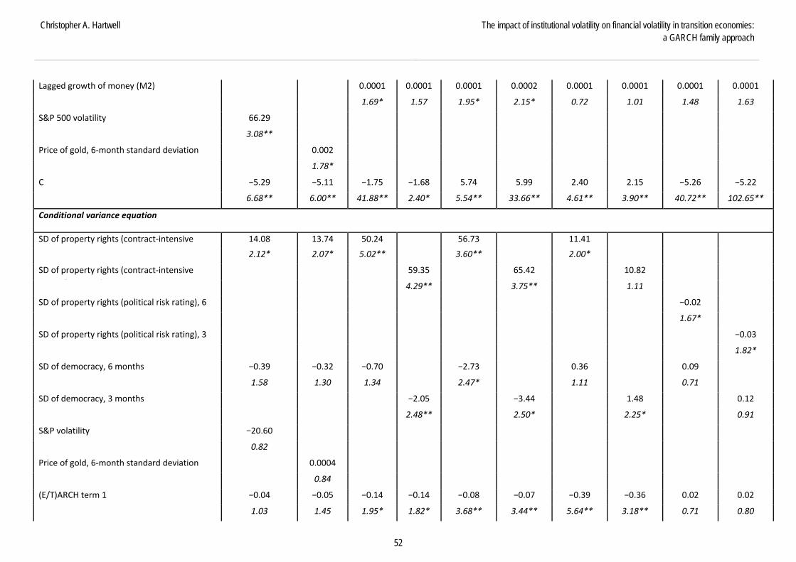
Christopher A. Hartwell The impact of institutional volatility on financial volatility in transition economies: a GARCH family approach
52
Lagged growth of money (M2) 0.0001 0.0001 0.0001 0.0002 0.0001 0.0001 0.0001 0.0001
1.69* 1.57 1.95* 2.15* 0.72 1.01 1.48 1.63
S&P 500 volatility 66.29
3.08**
Price of gold, 6-month standard deviation 0.002
1.78*
C −5.29 −5.11 −1.75 −1.68 5.74 5.99 2.40 2.15 −5.26 −5.22
6.68** 6.00** 41.88** 2.40* 5.54** 33.66** 4.61** 3.90** 40.72** 102.65**
Conditional variance equation
SD of property rights (contract-intensive
14.08 13.74 50.24 56.73 11.41
2.12* 2.07* 5.02** 3.60** 2.00*
SD of property rights (contract-intensive ) 3 h
59.35 65.42 10.82
4.29** 3.75** 1.11
SD of property rights (political risk rating), 6 h
−0.02
1.67*
SD of property rights (political risk rating), 3 h
−0.03
1.82*
SD of democracy, 6 months −0.39 −0.32 −0.70 −2.73 0.36 0.09
1.58 1.30 1.34 2.47* 1.11 0.71
SD of democracy, 3 months −2.05 −3.44 1.48 0.12
2.48** 2.50* 2.25* 0.91
S&P volatility −20.60
0.82
Price of gold, 6-month standard deviation 0.0004
0.84
(E/T)ARCH term 1 −0.04 −0.05 −0.14 −0.14 −0.08 −0.07 −0.39 −0.36 0.02 0.02
1.03 1.45 1.95* 1.82* 3.68** 3.44** 5.64** 3.18** 0.71 0.80

BOFIT- Institute for Economies in Transition Bank of Finland
BOFIT Discussion Papers 6/ 2014
53
(E/T)ARCH term 2 −0.11 −0.11 −0.18 0.20 −0.06 −0.09
3.34** 3.60** 2.84** 1.79* 2.98** 3.05**
EGARCH (Theta) 1 0.28 0.27 0.09 0.35 0.13 0.13
5.85** 5.93** 0.91 2.53* 3.03** 3.04**
EGARCH(Theta) 2 0.20 0.19 −0.28 −0.34 −0.04 −0.040
4.67** 4.54** 3.28** 2.22* 0.73 0.84
ABARCH term 1 0.54 0.54 0.11 0.12
9.64** 9.43** 3.16** 3.57**
EGARCH term 1 −0.67 −0.70 0.76 0.66 0.12 0.12
2.31* 2.68** 11.48** 7.18** 1.54 1.71*
EGARCH term 2 0.42 0.40 −0.47 −0.53 0.86 0.86
4.08** 4.19** 3.90** 4.98** 11.89** 12.48**
EGARCH term 3 0.69 0.72
2.55** 2.90**
EGARCH term 4 0.45 0.47
4.04** 4.60**
TGARCH term 1 0.53 0.49
3.40** 3.99**
TGARCH term 2 0.38 0.43
2.92** 4.15**
AR terms
AR(1) 0.43 0.45 0.45 0.44 0.46 0.47 1.10 1.13 0.45 0.45
17.54** 19.05** 25.46** 15.67** 19.46** 18.99** 80.81** 81.12** 20.82** 99.73**
AR(2) 0.12 0.13 0.10 0.10 0.12 0.12 −0.09 −0.14 0.12 0.12
4.94** 5.18** 4.44** 3.58** 4.94** 3.37** 6.70** 6.58** 5.33** 24.69**
AR(3) 0.04 2 0.04 0.04 0.07 0.08 −0.05 −0.03 0.01 0.01
1.71* 0.94 2.01* 1.44 3.03** 2.62** 1.55 2.09* 0.48 1.55

Christopher A. Hartwell The impact of institutional volatility on financial volatility in transition economies: a GARCH family approach
54
AR(4) 0.06 0.06 0.05 0.05 0.03 0.03 −0.02 0.00 0.06 0.06
2.37* 2.50* 2.89** 1.91* 1.20 0.69 0.50 0.07 3.10** 7.03**
AR(5) −0.002 −0.01 0.05 0.05 0.03 0.03 0.01 0.01 0.02 0.02
0.10 0.32 2.47* 1.96* 1.53 0.94 0.50 0.74 0.77 1.17
AR(6) 0.05 0.06 0.07 0.06 0.06 0.06 0.04 0.02 0.03 0.03
2.25* 2.29* 2.86** 2.29* 2.55* 2.53* 2.50* 1.56 1.48 3.11**
AR(7) 0.04 0.04 0.00 0.00 0.04 0.04 0.05 0.05
1.64 1.45 0.15 0.13 1.90* 1.35 1.98* 3.17**
AR(8) 0.06 0.07 0.07 0.07 0.04 0.06 0.06 0.08
2.71** 3.04** 5.38** 3.12** 2.01* 2.71** 2.86** 7.90**
n 2123 2123 2035 2047 2231 2245 2394 2409 2137 2140
Log likelihood −2657.316 −2659.23 −1101.58 −1107.22
−2780.59 −2793.03 −403.98 −436.95 −2586.41 −2590.91
AIC (Stata) 5368.631 5372.46 2243.163 2254.44
5605.182 5630.067 851.965 917.8943 5220.821 5229.814
AIC (normalized) 2.5288 2.5306 1.1023 1.1013 2.5124 2.5078 0.3559 0.3810 2.4431 2.4438
Jarque-Bera kurtosis statistic 3.489 3.467 4.022 4.137 4.342 4.284 21.98 17.39 3.739 3.72
Kolmogorov-Smirnov test p-statistic 0.389 0.151 0.768 0.897 0.164 0.162 0.00 0.00 0.04 0.04
Q test p-statistic 0.57 0.55 0.56 0.56 0.38 0.38 0.23 0.22 0.49 0.49
Distribution Student's T GED GED GED Student's T GED Student's T Student's T GED GED
Note: absolute values of t-stats are under the coefficients, with * signifying significance at the 10% level and ** at the 1% level.

BOFIT- Institute for Economies in Transition Bank of Finland
BOFIT Discussion Papers 6/ 2014
55
References
Acemoglu, D. and Johnson, S. (2005) Unbundling institutions. Journal of Political Econ-omy, 113(5), pp. 949–995.
Agenor, P.R., Aizenman, J. and Hoffmaister, A. (1998) Contagion, Bank Lending Spreads, and Output Fluctuations. National Bureau of Economic Research Working Paper, W6850.
Aizenman, J. and Marion, N.P. (1993) Policy Uncertainty, Persistence and Growth*. Re-view of International Economics, 1(2), pp. 145–163.
Akitoby, B. and Stratmann, T. (2010) The value of institutions for financial markets: evi-dence from emerging markets. Review of World Economics, 146(4), pp. 781–797.
Akomiv, A., Wijeweera, A. and Dollery, B. (2009) Financial Development and Economic Growth: Evidence from Transition Economies. Applied Financial Economics, 19, pp. 999–1008.
Ali, F. A., Fiess, N. and MacDonald, R. (2010) Do institutions matter for foreign direct investment? Open Economies Review, 21(2), pp. 201–219.
Andersen, T. G. (1996) Return volatility and trading volume: An information flow inter-pretation of stochastic volatility. The Journal of Finance, 51(1), pp. 169–204.
Andersen, T. G. and Bollerslev, T. (1998) Answering the sceptics: Yes, standard volatility models do provide accurate forecasts. International Economic Review, 39(4), pp. 885–905.
Andraz, J., and Norte, N. (2013) Output volatility in the OECD: Are the member states be-coming less vulnerable to exogenous shocks? Economic Issues Journal Articles, 18(2), pp. 91–122.
Andrianaivo, M. and Yartey, C.A. (2009) Understanding the Growth of African Financial Markets. IMF Working Paper 09/182.
Angelopoulos, K., Economides, G. and Vassilatos, V. (2011) Do institutions matter for economic fluctuations? Weak property rights in a business cycle model for Mexico. Review of Economic Dynamics, 14(3), pp. 511–531.
Arellano, M. and Bover, O. (1995) Another Look at the Instrumental Variable Estimation of Error-Components Models. Journal of Econometrics, 68, pp. 29–52.
Asoni, A. (2008) Protection of property rights and growth as political equilibria. The Jour-nal of Economic Surveys, 22(5), pp. 953–987.
Asteriou, D. and Price, S.G. (2001) Political Instability and Economic Growth: UK Time Series Evidence. Scottish Journal of Political Economy, 48, pp. 244–249.
Baker, S., Bloom, N. and Davis, S. (2013) Measuring economic policy uncertainty. Chi-cago Booth Research Paper, (13−02).
Baumol, W.J. (1990) Entrepreneurship: productive, unproductive and destructive. Journal of Political Economy, 98 (5), pp. 893–921.

Christopher A. Hartwell The impact of institutional volatility on financial volatility in transition economies: a GARCH family approach
56
Beck, T. and Demirgüç-Kunt, A. (2009) Financial Institutions and Markets Across Coun-tries and over Time: Data and Analysis. Policy Research Working Paper No. 4943, The World Bank.
Beck, T., and Levine, R. (2008) Legal institutions and financial development. Heidelberg: Springer Berlin, pp. 251–278.
Beck, T., Lundberg, M. and Majnoni, G. (2006) Financial intermediary development and growth volatility: Do intermediaries dampen or magnify shocks? Journal of Interna-tional Money and Finance, 25(7), pp. 1146–1167.
Beirne, J., Caporale, G.M., Schulze-Ghattas, M. and Spagnolo, N. (2009) Volatility Spill-overs and Contagion From Mature to Emerging Stock Markets. European Central Bank (ECB) Working Paper No. 1113, November.
Bekaert, G. and Harvey, C.R. (1997) Emerging equity market volatility. Journal of Finan-cial economics, 43(1), pp. 29–77.
Beltratti, A. and Morana, C. (2006) Breaks and persistency: macroeconomic causes of stock market volatility. Journal of Econometrics, 131(1), pp. 151–177.
Berggren, N., Bergh, A. and Bjørnskov, C. (2012) The Growth Effects of Institutional In-stability. Journal of Institutional Economics, 8(2), pp. 187–224.
Berglof, E. and Bolton, P. (2002) The Great Divide and Beyond: Financial Architecture in Transition. Journal of Economic Perspectives, 16, pp.77–100.
Besley, T. (1995) Property Rights and Investment Incentives: Theory and Evidence from Ghana. Journal of Political Economy, 103, pp. 903–937.
Białkowski, J., Gottschalk, K. and Wisniewski, T.P. (2008) Stock market volatility around national elections. Journal of Banking and Finance, 32(9), pp. 1941–1953.
Bloom, N. (2009) The impact of uncertainty shocks. Econometrica, 77(3), pp. 623–685.
Blundell, R., and Bond, S. (1998) Initial Conditions and Moment Restrictions in Dynamic Panel Data Models. Journal of Econometrics, 87, pp. 115–143.
Bollerslev, T. (1987) A conditional heteroskedastic time series model for speculative price and rate of return. Review of Economics and Statistics, 9, pp. 542–547.
Bollerslev, T. and Zhou, H. (2006) Volatility Puzzles: A Simple Framework for Gauging Return-Volatility
Regressions. Journal of Econometrics, 131(1), pp. 123–156. Bollerslev, T, Engle, R.F, and Nelson, D.B. (1994) ARCH models. In Handbook of Econometrics (Vol. IV), Engle RF, McFadder DL (eds). Elsevier Science: Amster-dam.
Boutchkova, M., Doshi, H., Durnev, A. and Molchanov, A. (2012) Precarious politics and return volatility. Review of Financial Studies, 25(4), pp. 1111–1154.
Boyd, J.H., Levine, R. and Smith, B.D. (2001). The impact of inflation on financial sector performance. Journal of Monetary Economics, 47(2), pp. 221–248.
Brailsford, T.J., and Faff, R.W. (1996) An Evaluation of Volatility Forecasting Tech-niques. Journal of Banking and Finance, 20(3), pp. 419–438.

BOFIT- Institute for Economies in Transition Bank of Finland
BOFIT Discussion Papers 6/ 2014
57
Braun, P.A., Nelson, D.B. and Sunier, A.M. (1995) Good news, bad news, volatility, and betas. The Journal of Finance, 50(5), pp. 1575–1603.
Brown, R. P., Carmignani, F. and Fayad, G. (2013) Migrants’ Remittances and Financial Development: Macro‐and Micro‐Level Evidence of a Perverse Relationship. The World Economy, 36(5), pp. 636–660.
Buiter, Willem H. (2003) Capital account liberalization and financial sector development in transition countries. In: Bakker, Age, and Chapple, Bryan, (eds). Capital liberali-zation in transition countries, lessons from the past and for the future. Edward El-gar, Cheltenham, UK, pp. 105–141.
Busse, M., and Hefeker, C. (2007) Political risk, institutions and foreign direct investment. European Journal of Political Economy, 23(2), pp. 397–415.
Campos, N. F., and Karanasos, M. (2008) Growth, Volatility, and Political Instability: Non-Linear Time-Series Evidence for Argentina, 1896−2000. Economics Letters, 100, pp. 135–137.
Catrinescu, N., Leon-Ledesma, M., Piracha, M. and Quillin, B. (2009) Remittances, Insti-tutions and Economic Growth. World Development, 37(1), pp. 81–92.
Cermeno, R. and Grier, K. (2006) Conditional heteroskedasticity and cross-sectional de-pendence in panel data: an empirical study of inflation uncertainty in the G7 coun-tries. In: B. Baltagi (ed.), Panel Data Econometrics: Theoretical Contributions and Empirical Applications. Springer: New York, pp. 259–278.
Chen, N.F., Roll, R. and Ross, S.A. (1986) Economic forces and the stock market. Journal of Business, 59, pp. 383–403.
Chinn, M.D. and Ito, H. (2006) What matters for financial development? Capital controls, institutions, and interactions. Journal of Development Economics, 81(1), pp. 163–192.
Chinn, M.D. and Ito, H. (2008). A New Measure of Financial Openness. Journal of Com-parative Policy Analysis, 10, pp. 309–322.
Chow, G.C. and Lin, A. (1971) Best linear unbiased interpolation, distribution, and ex-trapolation of time series by related series. Review of Economics and Statistics, 53(4), pp. 372–375.
Christie, A. A. (1982). The stochastic behaviour of common stock variances: value, lever-age and interest rate effects. Journal of Financial Economics, 10(4), pp. 407–432.
Chung, C.C. and Beamish, P.W. (2005) The Impact of Institutional Reforms on Character-istics and Survival of Foreign Subsidiaries in Emerging Economies. Journal of Management Studies, 42(1), pp. 35–62.
Claessens, S. and Laeven, L. (2003) Financial Development, Property Rights, and Growth. Journal of Finance, 58(6), pp. 2401–2436.
Clague, C., Keefer, P., Knack, S., and Olson, M. (1996) Property and contract rights in au-tocracies and democracies. Journal of Economic Growth, 1(2), pp. 243–276.
Clague, C., Keefer, P., Knack, S., and Olson, M. (1999). Contract-intensive money: con-tract enforcement, property rights, and economic performance. Journal of Economic Growth, 4(2), pp. 185–211.

Christopher A. Hartwell The impact of institutional volatility on financial volatility in transition economies: a GARCH family approach
58
Clemente, J., Montañés, A. and Reyes, M. (1998) Testing for a unit root in variables with a double change in the mean. Economics Letters, 59, pp. 175–182.
Compton, R.A. and Giedeman, D.C. (2011) Panel evidence on finance, institutions and economic growth. Applied Economics, 43(25), pp. 3523–3547.
Coricelli, F. and Maurel, M. (2011) Growth and Crisis in Transition: A Comparative Per-spective. Review of International Economics, 19, pp. 49–64.
Corradi, V., Distaso, W., and Mele, A. (2013) Macroeconomic Determinants of Stock Volatility and Volatility Premiums. Journal of Monetary Economics, 60, pp. 203–220.
Cottarelli, C., DellAriccia, G. and Vladkova-Hollar, I. (2005) Early birds, late risers, and sleeping beauties: Bank credit growth to the private sector in Central and Eastern Europe and in the Balkans. Journal of Banking & Finance, 29, pp. 83–104.
Dabla-Norris, E. and Srivisal, N. (2013) Revisiting the Link between Finance and Macro-economic Volatility. IMF Working Paper 13/29.
Daly, K. (2011) An Overview of the Determinants of Financial Volatility: An Explanation of Measuring Techniques. Modern Applied Science, 5, pp. 46–63.
Demirgüç-Kunt, A. and Detragiache, E. (1998) The Determinants of Banking Crises: Evi-dence from Industrial and Developing Countries. IMF Staff Papers, 45(1), pp. 81–109.
Demirgüç-Kunt, A. and Levine, R. (1996) Stock Market Development and Financial In-termediaries: Stylized Facts. The World Bank Economic Review, 10 (2), pp. 291–321.
Ding, Z., Granger, C.W.J., Engle, R. (1993) A Long Memory Property of Stock Market Returns and a New Model. Journal of Empirical Finance, 1, pp. 83–106.
Dollar, D., and Kraay, A. (2003) Institutions, trade, and growth. Journal of Monetary Eco-nomics, 50(1), pp. 133–162.
Dunis, C.L. and Shannon, G. (2005) Emerging markets of South-East and Central Asia: Do they still offer a diversification benefit? Journal of Asset Management, 6(3), pp.168–190.
Durham, J.B. (2002). The effects of stock market development on growth and private in-vestment in lower-income countries. Emerging Markets Review, 3, pp. 211–232.
Durnev, A., Errunza, V. and Molchanov, A. (2009) Property rights protection, corporate transparency, and growth. Journal of International Business Studies, 40(9), pp. 1533–1562.
Dutta, N., and Roy, S. (2011) Foreign direct investment, financial development and politi-cal risks. The Journal of Developing Areas, 44(2), pp. 303–327.
Egert, B., and Koubaa, Y. (2004) Modelling Stock Returns in the G-7 and in Selected CEE Economies: A Non-linear GARCH Approach. William Davidson Institute (Univer-sity of Michigan) Working paper Number 663, February.
Engle, R. F. (1982) Autoregressive Conditional Heteroskedasticity with Estimates of the Variance of U.K. Inflation. Econometrica, 50(4), pp. 987–1008.

BOFIT- Institute for Economies in Transition Bank of Finland
BOFIT Discussion Papers 6/ 2014
59
Engle, R.F. and Ng, V.K. (1993) Measuring and Testing the Impact of News on Volatility. The Journal of Finance, 48(5), pp. 1749–1778.
Engle, R.F., and Rangel, J.G. (2008) The Spline-GARCH Model for Low-Frequency Vola-tility and Its Global Macroeconomic Causes. Review of Financial Studies, 21 (3), pp. 1187–1222.
Errunza, V. and Hogan, K. (1998) Macroeconomic determinants of European stock market volatility. European Financial Management, 4(3), pp. 361–377.
Flannery, M. J., and Protopapadakis, A. A. (2002). Macroeconomic factors do influence aggregate stock returns. Review of Financial Studies, 15(3), pp. 751–782.
Fleming, J. (1998) The quality of market volatility forecasts implied by S&P 100 index option prices. Journal of Empirical Finance, 5(4), pp. 317–345.
Forbes, K.J. and Rigobon, R. (2002) No contagion, only interdependence: measuring stock market comovements. The Journal of Finance, 57(5), pp. 2223–2261.
Fortin, J. (2010) A tool to evaluate state capacity in post‐communist countries, 1989–2006. European Journal of Political Research, 49(5), pp. 654–686.
Friedman, M. (1977) Nobel lecture: inflation and unemployment. Journal of Political Economy, 85(3), pp. 451–472.
Fries, S. and Taci, A. (2002) Banking Reform and Development in Transition Economies. European Bank for Reconstruction and Development Working Paper No. 71, avail-able at:
http://www.ebrd.com/downloads/research/economics/workingpapers/wp0071.pdf.
Gabaix, X., Gopikrishnan, P., Plerou, V. and Stanley, H.E. (2006) Institutional investors and stock market volatility. The Quarterly Journal of Economics, 121(2), pp. 461–504.
Gallo, A.A. and Alston, L.J. (2008) Argentina's Abandonment of the Rule of Law and its Aftermath. Washington University Journal of Law & Policy, 26, pp. 153–182.
Garcia, V.F. and Liu, L. (1999). Macroeconomic Determinants of Stock Market Develop-ment. Journal of Applied Economics, 2(1), pp. 29–59.
Giannetti, M. and Ongena, S. (2009) Financial Integration and Firm Performance: Evi-dence from Foreign Bank Entry in Emerging Markets. Review of Finance, 13, pp. 181–223.
Gourinchas, P-O., Valdes, R. and Landerretche, O. (2001). Lending Booms: Some Stylized Facts. NBER Working Paper 8249, April.
Granger, C.W. and Swanson, N.R. (1997) An introduction to stochastic unit-root proc-esses. Journal of Econometrics, 80(1), pp. 35–62.
Hartwell, C.A. (2013) Institutional Barriers in the Transition to Market: Explaining Per-formance and Divergence in Transition Economies, London: Palgrave Macmillan.
Hayo, B. and Kutan, A.M. (2005) IMF-Related News and Emerging Financial Markets. Journal of International Money and Finance, 24, pp. 1126–1142.
Henisz, W. (2004) Political Institutions and Policy Volatility. Economics and Politics, 16(1), pp. 1–27.

Christopher A. Hartwell The impact of institutional volatility on financial volatility in transition economies: a GARCH family approach
60
Hsing, Y. and Hsieh, W-J. (2012) Impacts of Macroeconomic Variables on the Stock Mar-ket Index in Poland: New Evidence. Journal of Business Economics and Manage-ment, 13, pp. 334–343.
Jayasuriya, S. (2005) Stock market liberalization and volatility in the presence of favorable market characteristics and institutions. Emerging Markets Review, 6(2), pp. 170–191.
King, M.A. and Wadhwani, S. (1990) Transmission of volatility between stock markets. Review of Financial Studies, 3(1), pp. 5–33.
Kliesen, K.L., Owyang, M.T. and Vermann, E.K. (2012) Disentangling Diverse Measures: A Survey of Financial Stress Indexes. Federal Reserve Bank of St. Louis Review, 94(5), pp. 369–397.
Klomp, J. and de Haan, J. (2009) Political Institutions and Economic Volatility. European Journal of Political Economy, 25, pp. 311–326.
Knack, S. (1996) Institutions and the Convergence Hypothesis: The Cross-National Evi-dence. Public Choice, 87(3/4), pp. 207–228.
Knack, S. and Keefer, P. (1995) Institutions and economic performance: cross‐country tests using alternative institutional measures. Economics & Politics, 7(3), pp. 207–227.
Knack, S., Kugler, M. and Manning, N. (2003) Second-generation governance indicators. International Review of Administrative Sciences, 69(3), pp. 345–364.
Koutmos, G. and Booth, G.G. (1995) Asymmetric volatility transmission in international stock markets. Journal of international Money and Finance, 14(6), pp. 747–762.
Lawson, C. and Wang, H. (2005) Economic Transition in Central and Eastern Europe and the Former Soviet Union: Which Policies Worked? Centre for Public Economics at the University of Bath Working Paper No. 01−05.
Levitsky, S. and Murillo, M.V. (2009) Variation in institutional strength. Annual Review of Political Science, 12(1), pp. 115–133.
Lin, C., Lin, P. and Zou, H. (2012) Does property rights protection affect corporate risk management strategy? Intra- and cross-country evidence. Journal of Corporate Fi-nance, 18(2), pp. 311–330.
Loayza, N.V. and R. Ranciere (2006) Financial Development, Financial Fragility, and Growth. Journal of Money, Credit, and Banking, 38(4), pp. 1051–1076.
Lunde, A. and Hansen, P.R. (2005) A forecast comparison of volatility models: does any-thing beat a GARCH(1,1)? Journal of Applied Econometrics, 20(7), pp. 873–889.
Malik, F. (2011) Estimating the impact of good news on stock market volatility. Applied Financial Economics, 21(8), pp. 545–554.
Merton, R. (1980) On estimating the expected return on the market: An explanatory inves-tigation. Journal of Financial Economics, 8(4), pp. 323–361.
Miletkov, M., and Wintoki, M.B. (2012) Financial development and the evolution of prop-erty rights and legal institutions. Emerging Markets Review, 13(4), pp. 650–673.

BOFIT- Institute for Economies in Transition Bank of Finland
BOFIT Discussion Papers 6/ 2014
61
Moers, L. (1999). How Important are Institutions for Growth in Transition Countries? Tin-bergen Institute Discussion Papers 99−004/2, http://www.tinbergen.nl/discussionpapers/99004.pdf.
Murray, M.P. (2006) Avoiding Invalid Instruments and Coping with Weak Instruments. Journal of Economic Perspectives, 20(4), pp. 111–132.
Naaborg, I., Scholtens, B., De Haan, J., Bol, H. and De Haas, R. (2003) How Important are Foreign Banks in the Financial Development of European Transition Countries? CESifo Working Paper No. 1100,
http://www.cesifo-group.de/portal/pls/portal/docs/1/1189418.PDF.
Nelson, D.B. (1991) Conditional heteroskedasticity in asset returns: a new approach. Econometrica, 59, pp. 347–370.
North, D.C. (1971) Institutional Change and American Economic Growth. Cambridge University Press: New York.
Panetta, F. (2002) The Stability of the Relation between the Stock Market and Macroeco-nomic Forces. Economic Notes, 31(3), pp. 417–450.
Paye, B.S. (2012). ‘Déjà vol’: Predictive regressions for aggregate stock market volatility using macroeconomic variables. Journal of Financial Economics, 106(3), pp. 527–546.
Perry, P. (1982) The time-variance relationship of security returns: Implications for the re-turn-generating stochastic process. Journal of Finance, 37(3), pp. 857–870.
Ravn, M.O. and Uhlig, H. (2002) On adjusting the Hodrick-Prescott Filter for the fre-quency of observations. Review of Economics and Statistics, 84(2), pp. 371–375.
Rodrik, D. (1991) Policy uncertainty and private investment in developing countries. Jour-nal of Development Economics, 36(2), pp. 229–242.
Rodrik, D., Subramanian, A. and Trebb, F. (2004) Institutions Rule: The Primacy of Insti-tutions over Geography and Integration in Economic Development. Journal of Economic Growth, 9(2), pp. 131–165.
Rogers, J. M. and Siklos, P. L. (2003) Foreign exchange market intervention in two small open economies: the Canadian and Australian experience. Journal of International Money and Finance, 22(3), pp. 393–416.
Roodman, D. (2009) A Note on the Theme of Too Many Instruments. Oxford Bulletin of Economics and Statistics, 71(1), pp. 135–158.
Sachs, J.D. (2003). Institutions Don’t Rule: Direct Effects of Geography on Per Capita In-come. NBER Working Paper No. 9490 (February).
Schwert, G.W. (1989) Why does stock market volatility change over time? The Journal of Finance, 44(5), pp. 1115–1153.
Shibata, R. (1976) Selection of the order of an autoregressive model by Akaike’s informa-tion criterion. Biometrica, 63(1), pp. 117–126.
Stern, E., Sundelius, B., Nohrstedt, D., Hansén, D., Newlove, L. and Hart, P.T. (2002). Crisis management in transitional democracies: The Baltic experience. Government and Opposition, 37(4), pp. 524–550.

Christopher A. Hartwell The impact of institutional volatility on financial volatility in transition economies: a GARCH family approach
62
Stiglitz, J. (2002) Globalization and its Discontents. Norton, New York.
Svensson, J. (1998) Investment, property rights and political instability: Theory and evi-dence. European Economic Review, 42(7), pp. 1317–1341.
Tauchen, G. (1986) Statistical properties of generalized method-of-moments estimators of structural parameters obtained from financial market data. Journal of Business & Economic Statistics, 4(4), pp. 397–416.
Torstensson, J. (1994) Property Rights and Economic Growth: An Empirical Study. Kyk-los, 47(2), pp. 231–247.
Voigt, S. (2013) How (Not) to Measure Institutions. Journal of Institutional Economics, 9(1), pp. 1–26.
Wu, H.X. and Shea, E.Y.P. (2011) Explaining the China Puzzle: High Growth and Low Volatility in the Absence of Healthy Financial Institutions. Paper prepared for EcoMod2011, Azores, Portugal, June 29 – July 1, available online at: http://ecomod.net/system/files/Wu-Shea_EcoMod2011.pdf.
Yang, B. (2011) Political democratization, economic liberalization, and growth volatility. Journal of Comparative Economics, 39(2), pp. 245–259.
Yilmaz, R., Yabasakal, A., and Koyuncu, J. (2009) Foreign Bank Presence and Banking Crises in Transition Economies. Paper presented at EconAnadolu 2009: Anadolu In-ternational Conference in Economics, June 17−19,
http://econ.anadolu.edu.tr/fullpapers/Yilmaz_Yabasakal_Koyuncu_econanadolu2009.pdf.
Zakoian, J.M. (1994) Threshold Heteroskedastic Models. Journal of Economic Dynamics and Control, 18(5), pp. 931–955.

BOFIT Discussion Papers A series devoted to academic studies by BOFIT economists and guest researchers. The focus is on works relevant for economic policy and economic developments in transition / emerging economies.
BOFIT Discussion Papers http://www.bof.fi/bofit_en • email: [email protected]
ISSN 1456-6184, online
2013 No 1 Aaron Mehrotra: On the use of sterilisation bonds in emerging Asia No 2 Zuzana Fungáčová, Rima Turk Ariss and Laurent Weill: Does excessive liquidity creation trigger bank failures? No 3 Martin Gächter, Aleksandra Riedl and Doris Ritzberger-Grünwald: Business cycle convergence or decoupling? Economic adjustment in CESEE during the crisis No 4 Iikka Korhonen and Anatoly Peresetsky: What determines stock market behavior in Russia and other emerging countries? No 5 Andrew J. Filardo and Pierre L. Siklos: Prolonged reserves accumulation, credit booms, asset prices and monetary policy in Asia No 6 Mustafa Disli, Koen Schoors and Jos Meir: Political connections and depositor discipline No 7 Qiyue Xiong: The role of the bank lending channel and impacts of stricter capital requirements on the Chinese banking industry No 8 Marek Dabrowski: Monetary policy regimes in CIS economies and their ability to provide price and financial stability No 9 Rajeev K. Goel and Michael A. Nelson: Effectiveness of whistleblower laws in combating corruption No 10 Yin-Wong Cheung and Rajeswari Sengupta: Impact of exchange rate movements on exports: An analysis of Indian non-financial sector firms No 11 Martin Feldkircher, Roman Horvath and Marek Rusnak: Exchange market pressures during the financial crisis: A Bayesian model averaging evidence No 12 Alicia Garcia-Herrero and Le Xia: China’s RMB bilateral swap agreements: What explains the choice of countries? No 13 Markus Eller, Jarko Fidrmuc and Zuzana Fungáčová: Fiscal policy and regional output volatility: Evidence from Russia No 14 Hans Degryse, Liping Lu and Steven Ongena: Informal or formal financing? Or both? First evidence on the co-funding of Chinese firms No 15 Iikka Korhonen and Anatoly Peresetsky: Extracting global stochastic trend from non-synchronous data No 16 Roman Horvath, Jakub Seidler and Laurent Weill: How bank competition influence liquidity creation No 17 Zuzana Fungáčová, Laura Solanko and Laurent Weill: Does bank competition influence the lending channel in the Euro area? No 18 Konstantins Benkovskis and Julia Wörz: What drives the market share changes? Price versus non-price factors No 19 Marcel P. Timmer and Ilya B. Voskoboynikov: Is mining fuelling long-run growth in Russia? Industry productivity growth trends since 1995 No 20 Iftekhar Hasan, Liang Song and Paul Wachtel: Institutional development and stock price synchronicity: Evidence from China No 21 Iftekhar Hasan, Krzysztof Jackowicz, Oskar Kowalewski and Łukasz Kozłowski: Market discipline during crisis: Evidence from bank depositors in transition countries No 22 Yin-Wong Cheung and Risto Herrala: China’s capital controls – Through the prism of covered interest differentials No 23 Alexey Egorov and Olga Kovalenko: Structural features and interest-rate dynamics of Russia’s interbank lending market No 24 Boris Blagov and Michael Funke: The regime-dependent evolution of credibility: A fresh look at Hong Kong’s linked exchange rate system No 25 Jiandong Ju, Kang Shi and Shang-Jin Wei: Trade reforms and current account imbalances No 26 Marco Sanfilippo: Investing abroad from the bottom of the productivity ladder – BRICS multinationals in Europe No 27 Bruno Merlevede, Koen Schoors and Mariana Spatareanu: FDI spillovers and time since foreign entry No 28 Pierre Pessarossi and Laurent Weill: Do capital requirements affect bank efficiency? Evidence from China No 29 Irina Andrievskaya and Maria Semenova: Market discipline and the Russian interbank market No 30 Yasushi Nakamura: Soviet foreign trade and the money supply No 31 Anna Krupkina and Alexey Ponomarenko: Money demand models for Russia: A sectoral approach
2014 No 1 Vikas Kakkar and Isabel Yan: Determinants of real exchange rates: An empirical investigation No 2 Iftekhar Hasan, Krzysztof Jackowicz, Oskar Kowalewski and Łukasz Kozłowski: Politically connected firms in Poland and their access to bank financing No 3 Carsten A. Holz and Aaron Mehrotra: Wage and price dynamics in a large emerging economy: The case of China No 4 Zuzana Fungáčová, Anna Kochanova and Laurent Weill: Does money buy credit? Firm-level evidence on bribery and bank debt No 5 Jitka Poměnková, Jarko Fidrmuc and Iikka Korhonen: China and the World economy: Wavelet spectrum analysis of business cycles No 6 Christopher A. Hartwell: The impact of institutional volatility on financial volatility in transition economies: a GARCH family approach