Modelling and Forecasting Volatility of the BRICS Stock Markets: Evidence Using GARCH Models.

! 1!

School of Economics and Finance

Queen Mary University of London

Modell ing and Forecasting Volatil ity of the BRICS Stock

Markets: Evidence Using GARCH Models.

By

ANDRIA PERATITI

090448124

20/08/2013

Supervisors:

Dr. Leone Leonida

Dr. Dario Maimone Ansaldo Patti

Word Count: 5983

! 2!

Abstract

A number of previous studies have used ARCH and GARCH models in order to conclude on

the most appropriate model for estimating and forecasting volatility. In attempt to contribute to

literature, this study is devoted to find the most accurate heteroskedastic model for estimating

and forecasting volatility in the five main emerging economies: Brazil, Russia, India, China and

South Africa (BRICS) using daily equity indices. The empirical investigation is conducted

using various models from the GARCH-family. The models employed in this dissertation are

the GARCH (1,1), TGARCH (1,1,1), EGARCH (1,1) and the GARCH-M (1,1) with both

standard deviation and conditional variance in the mean equation.

The findings reveal that the TGARCH (1,1,1) model followed by EGARCH (1,1) model is

best suited for estimating and forecasting volatility. The results also suggest the presence of

leverage effects in the data. GARCH-M (1,1) is inappropriate for both modelling and

forecasting volatility in the emerging economies, as the risk-reward relationship is not detected.

! 3!

Table of contents:

ABSTRACT………………………………......……………...….…………….……2

TABLE OF CONTENTS………………………………..………..…….………..…3

ACKNOWLEDGEMENT………………………………..………………….…......5

SECTION I: INTRODUCTION………………………….………....…...…………6

SEDTION 2: LITERATURE REVIEW……………………..……...……...……....7

SECTION 3: DATA………………………...……..……………......…………...….9

SECTION 4: METHODOLOGY…………….…………………...………………..9

4.1: DATA BEHAVIOUR…………………..………………………………9

4.2: ESTIMATING VOLATILITY MODELS…………………..………...10

4.3: FORECASTING VOLATILITY………………..……………….…….12

SECTION 5: ESTIMATION RESULTS…………………..………………….......15

5.1: PRELIMINARY ANALYSIS………………………..….………….....15

5.2: MODEL ESTIMATION………………..………………………..….....19

5.3: FORECASTING EVALUATION……………..…………….………...24

SECTION 6: CONCLUSIONS………..………….……………………………….28

REFERENCE………..………………………………………….…………………29

! 4!

List of tables:

TABLE 1: Descriptive statistics for daily return series.............................................................. 15

TABLE 2: Autocorrelation test……………...……………………………………………….…19

TABLE 3.Test for “ARCH-effects” for daily returns……………………….……...……….….19

TABLE 4A: Coefficient estimates of GARCH (1,1)………………………...…….…...………20

TABLE 4B: Coefficient estimates of GARCH-M(1,1) with the conditional standard deviation

term in the mean……………………………………...…………………….……...….………...21

TABLE 4C: Coefficient estimates of GARCH-M (1,1) with the conditional variance term in the

mean………………………………..…………………………….……...……………………….21

TABLE 4D: Coefficient estimates of TGARCH(1,1,1)………………...……………………...22

TABLE 4E: Coefficient estimates of EGARCH(1,1)……………...…………………………..22

TABLE 5: Akaike Information Criterion………………………………………………..……..23

TABLE 6: Diagnostics in the standardized residuals………………………………………..…23

TABLE 7: RMSE measures from forecasting daily equity return volatility…………………...25

TABLE 8: MAPE measures from forecasting daily equity return volatility………………..….25

TABLE 9: MAE measures from forecasting daily equity return volatility.……………………25

List of figures:

Figures 1a-1e: Histograms of daily returns…………….……………...….……………….........16 Figures 2a-2e: Performance of daily returns………………..……...…..…………………...17-18

Figures 3a-3e: Plots of proxy against forecasted volatility…………..……..………………26-27

! 5!

Acknowledgement

The author wishes to express appreciation to her supervisor Dr Leone Leonida and her

Teaching Assistant Mr Davide Cafaro for their support during the process of this

dissertation.

Special thanks should go to Dr Dario Maimone Ansaldo Patti for his valuable guidance

and help.

The author also wants to thank five people important to her, who know who they are, for

their encouragement and love throughout this year.

! 6!

1: Introduction

Many academics and researchers have extensively discussed the importance of volatility

forecasting over the years. Akgiray (1989), states that volatility forecast is significant as it

provides evidence for the usefulness of the GARCH-type models as evaluation instruments of

the stock market. Volatility is an input in the Black-Scholes-Merton pricing formula for

determining the price of call and put options trading on an exchange. Hence, an accurate

forecast would be useful for pricing financial securities correctly. Tsay (2005), in his book,

explains more reasons for the importance of modelling and forecasting volatility. As he states,

another financial function of volatility is that it offers a simple method for calculating the Value

at Risk (VaR) in risk management. In addition it has a leading role in asset allocation under the

mean-variance relationship for investment decisions. Finally, the Volatility Index of market has

recently become a financial instrument (VIX). Therefore, forecasting the volatility of time

series makes parameter estimation more efficient as well as the interval forecast more accurate.

In finance, volatility is measured by standard deviation σ or variance σ2 from a size sample n

as! !! = !

!!! !! − !)!!!!! (1)

where µ is the mean return.

The purpose of this dissertation is to examine some of the linear, non-linear and asymmetric

econometric models for modelling and forecasting volatility of equity returns in BRICS and

conclude upon whether the predictive ability of a model outperforms the forecasting power of

the other models. Furthermore this study is interested on whether there has been a

chronological improvement in the literature’s models’ ability to forecast volatility. BRICS is

the abbreviation given to the five main emerging countries in the world: Brazil, Russia, India,

China and South Africa since 2010. Although the literature that focuses on the forecasting

ability of volatility models in developed economies is immense, little has been found for the

case of developing economies and even less for these five major emerging economies of the

world. The models tested in this paper are the Generalised ARCH (GARCH), Threshold

GARCH (TGARCH), Exponential GARCH (EGARCH) and the GARCH-in-mean (GARCH-

M) with both standard deviation and conditional variance in the mean equation.

This study is structured as follows: Section 1 is the introduction, which presents the aims

and motivation of this dissertation. It also mentions some important background information

about the topic. Section 2 discusses and analyses the main literature available for this topic. A

clarification of how this dissertation fits within the literature is presented. Section 3 describes

the data and Section 4 the methodology engaged in this dissertation. Section 5 demonstrates

and analyses the empirical findings. Section 6 is the conclusion part, which reviews the results

for the superiority of a certain model over the others.

! 7!

2.#Literature#Review#There is extensive literature that focuses on the evaluation of different models for modelling

and forecasting volatility in developed and emerging economies. This dissertation only focuses

on the GARCH-family models and more specifically on the performance of the linear, non-

linear and asymmetric GARCH models for the emerging economies of Brazil, Russia, India,

China and South Africa.#Song et al (1998) examined the relationship between returns and volatility for the emerging

Chinese stock markets. The main conclusion is that GARCH-M (1,1) specification explains

return series in the best way. The existence of time-varying risk premium in the emerging

markets of Latin America has also been observed by De Santis and Imrohoroglu (1997).

In the context of modelling volatility, Haroutounian and Price (2001) and Siourounis (2002)

concluded that the linear GARCH model estimates volatility in the most suitable way.

Alagidede and Panagiotidis (2009) studied the stock returns for 7 markets in Africa, including

South Africa. They concluded that GARCH, GARCH-M and EGARCH-M models estimate the

conditional variance properly.#Several researches questioned the superiority of the linear GARCH model in terms of its

forecasting power. Akgiray (1989) concluded that the GARCH (1,1) model is superior to the

other models for forecasting monthly US stock indices. West and Cho (1995) agree with the

choice of the linear model when forecasting volatility using dollar exchange rates. On the other

hand, Tse (1991) and Tse and Tung (1992), studying the Japanese and Singaporean stock

market respectively, concluded that Exponentially Weighted Moving Average (EWMA) model

has more forecasting ability than the ARCH/GARCH models. #The forecasting power of ARCH-type models was examined by Hansen and Lunde (2005).

They compared 330 ARCH-type models using DM–$ exchange rate data and IBM return data.

They found evidence of superiority of GARCH (1,1) model to more sophisticated models when

the evaluation is based on exchange rates, and inferiority of GARCH (1,1) modek when the

analysis is based on IBM returns. Finally, the study suggests that a model is superior to other

models for out-of-sample evaluation when it accommodates a leverage effect.

Although Dimson and Marsh (1990) did not examine the volatility forecast ability of the

(G)ARCH- family models, their conclusion gives an important implication for the forecasting

power of complex GARCH models. They proposed that more complex non-linear and non-

parametric models are more probable to underperform than parsimonious linear models. They

recommended the Exponential Smoothing model and the Regression model for forecasting

quarterly volatility.

Huang (2011) presents an extensive assessment of volatility models by investigating 31

markets. The findings of this assessment showed that for both the developed and developing

! 8!

economies, the GARCH models provide weak forecasting ability. In addition, the Stochastic

Volatility model gives the most accurate forecasts.#Some studies have shown that asymmetric models produce weak forecasts. Examples

include Brooks (1998) in the case of New York Stock Exchange and Franses and Van Dijk

(1996) in the case of five developed countries. Similarly, Xu (1999) who focused his research

on the Chinese market concluded that the symmetric model outperforms the EGARCH and

GJR-GARCH models. He observed that generally it is hard to use any GARCH-type models

for forecasting purposes as volatility in Shanghai is mostly influenced by governmental policy

on stock markets.#Gokcan (2000) extended Franses and Van Dijk (1996) study by investigating seven

emerging countries including Brazil. He concluded that GARCH (1,1) model has stronger

forecasting power than the EGARCH model, even though the return series are asymmetric.

McMilan et al (2000) using UK daily, weekly and monthly indices and Day and Lewis (1992)

using S&P 100 index have shown the superiority of the GARCH model when compared to the

EGARCH model.

On the other hand, there is vast literature suggesting that the role of asymmetry in volatility

forecasting is very important. Poon and Granger (2003) and Liu and Huang (2010) concluded

that asymmetric GARCH models perform better than the linear GARCH model. Similarly,

Awartani and Corradi (2005) employed daily S&P-500 Composite Price Index and suggested

that for one-step-ahead and longer time horizons, asymmetric GARCH models outperform the

GARCH (1,1) model. Furthermore, Carvalhal and Mendes (2008) tested the forecasting

performance of seven econometric models for the emerging markets in Latin America and Asia

including Brazil and India. They found that for in-sample estimation TGARCH and EGARCH

outperform the other models whilst the ARMA model has the best forecasting ability for out-

of-sample estimations.

Moreover, many authors showed that EGARCH model gives more accurate results than the

predictions given by the other asymmetric GARCH models. (Pagan and Schwert, 1990; Alberg

et al, 2008; Miron and Tudor, 2010; Shamiri and Isa, 2009; Chong et al, 1999)

Along the same lines, Brailsford and Faff (1993,1996) and Forte and Manera (2002) found

that for the Australian returns and for the data of ten European Stock Markets respectively,

GJR-GARCH model provides smaller forecasting errors. Finally, Engle and Ng (1993) when

examined the Japanese Stock Market concluded that GJR-GARCH and EGARCH models give

the most accurate forecasts.!

! 9!

3. Data

The data extracted for the purpose of this dissertation comprise 2610 daily equity

observations for each of the following countries: Brazil, Russia, India, and South Africa and

1891 daily equity observations for China. The data available for Brazil, Russia, India and South

Africa cover a period of 9 years and start from 1/4/2002 to 30/3/2012, while for China the

available data start from 31/12/2004 to 30/3/2012 and cover a period of 7 years and 3 months.

The sample period is divided into two sub-samples. The in-sample includes all the equity index

returns for the period of 1/4/2002 to 31/3/2011 for Brazil, Russia, India and South Africa and

for the period of 31/12/2004 to 31/3/2011 for China. These data are used for estimating the

models. The out-of-sample includes daily returns for the period of 1/4/2011 to 30/3/2012 for all

the countries, and is used to investigate the volatility forecasting power of the models.

The following daily equity indices of the BRICS Stock Exchange markets have been used:

Brazil’s BM&FBOVESPA, Russia’s Moscow Interbank Currency Exchange (MICEX), India’s

Bombay Stock Exchange (BSE), China Security Index 300 (CSI 300) and South Africa’s

FTSE/JSE. The data has been extracted from the Macrobond data set of the Excel add-in

function.

The high-frequency data turns out to be highly predictable and more accurate for ex-post

interdaily volatility evaluation (Andersen and Bollerslev, 1998). The use of daily observations

for examining the volatility forecasting ability of different models in the emerging economies is

compatible with literature (Song et al, 1998; Xu, 1999; Siourounis, 2002; Su and Knowes,

2006; Huang, 2011).

4. Methodology

4.1. Data Behaviour

Before conducting the main analysis and in order to make the time series stationary, the

daily returns Rt are defined as the first log-difference of each index’s value for two successive

days times 100. Hence, the continuously compounded daily returns (Rt) at time t are calculated

as:

!! = 100 !"#(!!)− !"#!(!!!!) = 100 !"# !!!!!!

(2)

for t = 1,…,2609 for all the countries except China and for t=1,…1890 for the latter. Pt is the

equity index at time t, for t =0,…,2610 for all the countries except China and for t =0,…,1891

for China.

Mandelbrot (1963) stated, “Large changes tend to be followed by large changes - of either

sign- and small changes tend to be followed by small changes ”. This is referred by academics

as volatility clustering and is one of the apparent patterns of financial time series, the so-called

stylized facts about volatility. Cont (2001) suggests that the other main features that

! 10!

characterize return series are: skewness, leptokurtosis, and volatility persistence and volatility

clustering. It is necessary that a preliminary analysis be conducted in order to decide if the

GARCH-family models can be employed since theory suggests that these models capture the

features stated above. Preliminary analysis is conducted by inspecting the descriptive statistics,

the absolute return series, and the variance of the daily returns and the autocorrelation of the

squared returns.#

4.2. Estimating Volatility Models Engle (2001) stated in his paper: “ARCH and GARCH models treat heteroskedasticity as a

variance to be modeled”. Therefore, it is important to compute the Engle (1982) test to

determine the presence of “ARCH effects” in the error terms. This can also be thought as

testing for the presence of conditional heteroskedasticity in the error terms. The first step is to

run the linear ARMA (1,1) model and obtain the residuals !!. Then to test for ARCH of order

five the residuals are squared and regressed on five lags as shown in the following equation:

!!! = !! + !!!!!!!! + !!!!!!!! +⋯+ !!!!!!! + !! (3)

where !! is an error term. Both the LM-test and the F-test are used to check for

heteroskedasticity. If heteroskedasticity is detected then the ARCH estimation method should

be used instead of the OLS method.

In the presence of heteroskedasticity, the five models used to estimate the conditional

variance are GARCH (1,1), TGARCH (1,1,1), EGARCH (1,1) and GARCH-M (1,1) with both

standard deviation and conditional variance in the mean equation. These models have been

extensively used in the literature due to their uncomplicatedness and verified ability to forecast

volatility. The statistical software used for estimating and forecasting the models is Eviews 7. When explaining the ARCH model, Engle (1982) stated that “for real processes one might

expect better forecast intervals if additional information from the past were allowed to affect

the forecast variance; a more general class of models is desirable” This has inspired Bollerslev

(1986) and Taylor (1986) to extend the ARCH model to the Generalised ARCH (GARCH)

model by allowing the conditional variance process simulate the ARMA process. One of the

reasons that the linear GARCH model is so popular is that it can effectively capture both the

volatility-clustering effect and the excess kurtosis in return series. The model is more

parsimonious in the estimation of the parameters and so less likely to violate the non-negativity

constraint. GARCH (1,1) is the most common model used for equity return data and has

conditional variance equation:

ℎ! = !! + !!!!!!! + !ℎ!!! (4)

where !! is the ARCH coefficient, ! is the GARCH coefficient and !! is the residual at time t.

The advantage of using it comes from the fact that it does not consider only the information

! 11!

about volatility from the previous period (!!!!!!! ) but also information coming from the fitted

values of the last period’s variance (!ℎ!!!). Chou (1988) proposed that when the sum of the

ARCH and GARCH parameters !! + ! is unitary then the shocks to volatility persist

infinitely and the model does not determine the unconditional variance. The fact that the linear GARCH model does not allow for any relationship between the

variance and the mean of returns, non-linear GARCH models have been suggested as a

consequence of the perceived problems. The GARCH-in-mean (GARCH-M) model suggested

by Engle, Lilien and Robins (1987) includes the conditional variance as another regressor to the

mean equation and thus allows ℎ! to have mean effects. The GARCH-M model is given by the

specification:

!! = ! + ! ℎ!!! + !! (5.1)

and

ℎ! = !! + !!!!!!! + !ℎ!!! (5.2)

where, !! ∼! 0, ℎ! , !! is the equity index return and µ is the mean. The parameter δ is

called the time varying risk premium. If δ is positive and statistically significant then, the

model is able to explain the volatility in the returns and it should be employed for forecasting

purposes.

In equity markets, stock prices are negatively correlated with volatility. This tendency of

volatility to increase more following a negative shock than following a positive one of the same

magnitude is named leverage effect (Black, 1976). To account for this phenomenon two

asymmetric models that capture this tendency of volatility are also estimated: TGARCH and

EGARCH. By estimating and testing the significance of the asymmetric terms one can

conclude on whether TGARCH and EGARCH models fit the data appropriately. The Threshold GARCH (TGARCH) of Glosten, Jagannathan and Runkle (1993) and

Zakonian (1994) accounts for possible asymmetries with the addition of a dummy variable in

the simple GARCH model. The conditional variance equation of TGARCH (1,1,1) is given by:

ℎ! = !! + !!!!!!! + !ℎ!!! + !!!!!! !!!! (6)

where !!!! is a binary dummy variable taking the value of 1 if !!!! < 0 and zero otherwise. As

Enders (2004), states in his book !!!! = 0 is a threshold and any innovations below or above

this have different effects on volatility. When the market moves upwards (!! > 0), conditional

variance is influenced by !!, while when the market moves downwards (!! < 0), volatility is

changed by !! + !. This leads to the implication that in the presence of leverage effects, ! is

strictly greater than zero and so higher volatility is observed when negative shocks happen.

When !!takes any other value than zero, the changes in the market are asymmetric. The Exponential GARCH (EGARCH) proposed by Nelson (1991) estimates the natural

logarithm of conditional variance. Therefore, even if the parameters are negative, ℎ! will

! 12!

always be positive. Thus, there is no need to artificially impose non-negativity constraints on

the model’s parameters, except ! < 1. Finally, the logarithm of the conditional variance

implies that, the leverage effect is exponential, in comparison with the TGARCH that is

quadratic. There are various ways to express the conditional variance equation of EGARCH

(1,1). One possible specification is:

!" ℎ! = !! + !"# ℎ!!! + ! !!!!!!!!

+ !! !!!!!!!!

− !! (7)

The parameter ! captures the asymmetry of the returns. Since asymmetries are allowed

under the EGARCH formulation, and the relationship between volatility and returns is

negative, in the presence of leverage effect ! is strictly smaller than zero. In order to decide on the appropriateness of the GARCH models the Akaike’s Information

Criterion (AIC) is used. For each model’s estimation table produced by Eviews software, the

corresponding AIC value is given. The most appropriate model minimises the value of the

Information Criterion. In order to estimate the Information Criterion value, Eviews software

uses the formula:

!"# = −2! ! + !!! (8)

where l is the log likelihood, T is the sample size and k is the number of the parameters.

To distinguish the best fit data model out of the appropriate GARCH models, diagnosis tests

are conducted. This study follows the diagnosis tests employed by Song et al (1998). The

standardised residual series of a suitable fit GARCH model should follow a normal distribution

and hence to have skewness and kurtosis coefficients close to zero and three respectively.

Therefore, the p-value of the Jarque-Bera statistic should be larger than 0.05 in order to not

reject, at 5% level, the null hypothesis that the errors are normally distributed. The Ljung-Box

cumulative statistic up to twelve lags is also employed to test the presence of autocorrelation in

the standardised residuals. The best fit model should fail to reject the null hypothesis of no

autocorrelation in the standardised residuals up to twelve lags.

4.3. Forecasting Volatility

Once the models with significant parameters have been estimated, they can be used to

derive one-year-ahead volatility forecasts. The idea behind forecasting volatility using the

GARCH-family models is that by theory, the conditional variance of the value of the return

series at each time period, given its prior values, is identical to the conditional variance of the

disturbance term for the same period, given its prior values (Brooks, 2008). This fact along

with the ability of the GARCH models to explain movements in the conditional variance of the

disturbance term infers that the forecasts of the conditional variance of each model are the

variance forecasts of the return series (Brook, 2008). Forecasts are produced for the whole of

! 13!

the out-of-sample period from 1/4/2011 to 30/3/2012 for all the five countries. The method

used for the forecasts is dynamic. In other words, multi-step-ahead procedure is carried out

starting on the first period of the out-of-sample and generating forecasts for one-, two-, and up

to s-steps-ahead, so that the forecasting interval is for the next s periods. It is important to note

that if the residual terms are not available for the forecast procedure of this dissertation, the

terms are replaced by their actual values. For the case of GARCH (1,1) model, with conditional variance equation:

ℎ!= !!+!!!!!!! + !ℎ!!! (9.1)

where all the coefficient estimates are known and the data are available up to and including

time T, the one-step-ahead forecast is calculated as:

ℎ!!!= !!+!!!!! + !ℎ! (9.2)

Given ℎ!!!, the two-step-ahead forecast is defined by the equation:

!ℎ!!! = !! + !!ℎ!!! + !ℎ!!!= !! + (!! + !)!ℎ!!! (9.3)

Finally, the s-step-ahead forecast is produced by:

!ℎ!!! = !! (!! + !)!!!!!!!!! + (!! + !)!!!ℎ!!! (9.4)

where s ≥ 2. The other models produce forecasts similarly. In order to determine the accuracy of a forecast, evaluation tools must be employed.

According to Bollerslev et al (1994), the most important forecast evaluation measure is the

economic loss function. However, it is usually unavailable so statistical loss function is used

instead. Following Chu and Freund (1996) and Brailsford and Faff (1996), the one-year-ahead

forecasts are assessed by the Root Mean Squared Error (RMSE), the Mean Absolute Error

(MAE) and the Mean Absolute Percentage Error (MAPE) defined as:

!"#! = !!!(!!!!)

(!!!! − ℎ!!!)!!!!!! (10)

!"# = ! !!!(!!!!)

!!!! − ℎ!!!!!!!! (11)

!"#$ = ! !""!!(!!!!)

!!!!!!!!!!!!!

!!!!! (12)

where ℎ!!!!is the s-step-ahead volatility forecasts of the equity index at time t, !! is the actual

volatility at time t, T is the total sample size and T1 is the first out-of sample forecast

observation. RMSE is an orthodox error statistic that gives a harsh penalty on large forecast

errors. MAE is a conventional forecast criterion that gives the same weight to all forecast

errors, while MAPE is interpreted as a percentage error and its value cannot get negative.

Makridakis (1993) claims that MAPE is the most accurate statistical loss function. In terms of

analysis, the lower the value of RMSE and MAE is, the more accurate the model is in terms of

forecasting, while the closer to 100% the value of MAPE is, the better the model predicts

volatility. Finally, in order to see how well each model tracks price changes, the forecasted volatility is

! 14!

compared to the actual volatility. Due to the fact that actual volatility is unobservable, squared

daily returns are used as a proxy of actual volatility. Squared returns are an unbiased but very

noisy estimator of ex post volatility (Lopez, 2001). Since the squared daily returns are only

used for comparison reason, their imprecise characteristic does not imply that the inferences

made are incorrect because they are unbiased. The choice of squared daily returns as a proxy of

actual volatility is consistent with literature. Brailsford and Faff (1996) and Awartani and

Corradi (2005) have also used this evaluation method.

! 15!

5. Estimation Results

5.1Preliminary Analysis

By inspecting the summary statistics presented in Table 1 it can be seen that the mean and

the median of all the five countries is positive and not significantly different from zero,

implying that equity returns increase slightly as time passes. Furthermore, the large difference

between the minimum and the maximum values of the returns indicate that large changes in

volatility often occur in the BRICS countries. De Santis and Imrohoroglu (1997) when

examining the volatility of the emerging economies including Brazil, India and China found

similar results. High volatility, measured by standard deviation, is accompanied by high

average daily returns. This is a common observation in the emerging economies and is

consistent with Shamiri and Isa (2009). In fact, South Africa has the lowest mean and standard

deviation value while Russia is the most volatile country with the highest average returns.

The Gaussian distribution of the return series is not a phenomenon in the emerging markets’

data (Choudry, 1996; Gokcan, 2000; Kurma, 2006). This study is consistent with literature

observing leptokurtic and skewed residuals. In a Gaussian distribution the coefficients of

skewness and kurtosis should be zero and three correspondingly. The coefficients of kurtosis,

which are much larger than three, indicate the leptokurtic distribution of the residuals, while the

negative, but very close to zero, coefficients of skewness imply that market falls more frequent

than it rises. So, the equity returns follow a non-normal distribution mostly because of the

excess kurtosis presented in the residuals rather than skewness. Finally, the null hypothesis of

the Jarque- Bera statistic that the residuals follow a normal distribution is strongly rejected at

1% significance level as the p-value in all cases is zero. This means that the implications made

for coefficient estimates could be incorrect. The fact that the sample is large makes this concern

less severe.

Non-normality is also supported by visually inspecting the histograms (see Figures 1a-1e).

As it can be seen none of them has a bell-shape, instead they are all asymmetric with a longer

tail on the left. Bolleslev et al (1994) stated that the non-constant variance of the time-

dependent series produces leptokurtosis, which links volatility clustering with non-normal

distribution.

! 16!

Figure 1a. Histogram of daily returns for Figure 1b. Histogram of daily returns for

Brazil (1/4/2002-31/3/2011) Russia (1/4/2002-31/3/2011)

Figure 1c. Histogram of daily returns for Figure 1d. Histogram of daily returns for

India (1/4/2002-31/3/2011) China (31/12/2004-31/3/2011)

Figure 1e. Histogram of daily returns for

South Africa (1/4/2002-31/3/2011)

Another important feature of financial returns is the volatility clustering. As it can be seen

from Figures 2a-2e volatility in BRICS occurs in bursts. The daily return series of South Africa

appears to be the most volatile in this period of time. In general slight tranquility is recorded for

all the countries over the time-span. Inevitably due to the U.S housing boom far more volatility

has been recorded in mid-2008 till 2009 for all the countries with many large positive and

negative returns in such a small time interval. Finally, the non-constant variance suggests the

consideration of heteroskedasticity when estimating the models.

0

100

200

300

400

500

600

700

800

-5 -4 -3 -2 -1 0 1 2 3 4 5 6

Series: DAILYRETURNSSample 4/01/2002 3/31/2011Observations 2349

Mean 0.030391Median 0.025384Maximum 5.940376Minimum -5.253256Std. Dev. 0.818362Skewness -0.094643Kurtosis 8.005594

Jarque-Bera 2455.860Probability 0.000000

0

100

200

300

400

500

600

-3 -2 -1 0 1 2 3




0

50

100

150

200

250

300

350

400

-4 -3 -2 -1 0 1 2 3 4




0

100

200

300

400

500

600

700

800

-8 -6 -4 -2 0 2 4 6 8 10




0

200

400

600

800

1,000

-4 -2 0 2 4 6




! 17!

Figure 2a. Daily returns of Brazil (1/4/2002-31/3/2011)

Figure 2b. Daily returns of Russia (1/4/2002-31/3/2011)

Figure 2c. Daily returns of India (1/4/2002-31/3/2011)

! 18!

Figure 2d. Daily returns of China (31/12/2004-31/3/2011)

Figure 2e. Daily returns of South Africa (1/4/2002-31/3/2011)

Finally, Table 2 reports the Ljung-Box Q-statistic with the relevant probabilities for the first,

sixth and twelfth lags under the joint null hypothesis of no serial correlation in the squared

returns up to each lag. The table also presents the autocorrelation coefficients at each lag. It is

obvious that small positive first-order autocorrelations are present in all the countries. These

results are consistent with the results found by Gokcan (2000) for the case of seven emerging

markets and validate the employment of GARCH-type specifications for the estimation of

volatility models. The actual correlograms can be found in Appendix 1.

! 19!

5.2 Model Estimation

After the ARMA(1,1) model has been estimated, the presence of conditional

heteroskedasticity in the residuals is examined in order to decide whether the ARCH estimation

method is more suitability than the OLS method for modeling the data. The values of the F-test

and the LM-test are synopsized in Table 3. Actual tables can be found in Appendix 2.

Both the LM-test and the F-statistic, in all the emerging markets have a probability value of

0. Therefore, the null hypothesis of homoscedasticity of errors, denoted as

H0:γ1=γ2=γ3=γ4=γ5=0, is rejected at 1% significance level, suggesting the presence of ARCH

effects in the residuals and so the presence of volatility clustering in the returns. Hence

GARCH specifications should be employed for modeling the volatility of the BRICS Exchange

market. Ortij (2001) and Chong et al (1999) have also found evidence of ARCH effects in other

emerging economies.

Tables 4A-4E synopsize the coefficient estimates along with their probabilities and standard

errors for each model for all the five countries together. These findings are used in the

! 20!

empirical analysis in order to establish the superiority of a model for estimating volatility.

Actual Tables can be found in Appendix 3.

For GARCH (1,1) model, the constant (!!), the lagged squared residual (!!) and the lagged

conditional variance (β) in the conditional variance equation are positive and highly significant

for all the countries. The mean coefficients (µ) are also statistically significant at 1% level.

Since all the parameters are positive, the non-negativity condition of the GARCH models is

satisfied. The fact that the value of the ARCH parameter is much smaller than the value of the

GARCH parameter signifies high persistence with little expected deviations. The high

persistence of shocks to conditional variance can be seen by the fact that the sum of the

persistence parameters (α1 + β) is close to one. De Santis and Imrohoroglu (1997) and Song et

al (1998) found similar results regarding the high persistence of shocks to volatility in the case

of other emerging economies. The above observations are presented in the Table 4A:

Tables 4B and 4C display the findings for the GARCH-M (1,1) model with conditional

standard deviation and conditional variance term in the mean respectively. Generally, the

coefficient estimates in the volatility equation of the GARCH-M (1,1) model in both cases are

highly statistically significant. On the other hand, the standard deviation and the conditional

variance in the mean equation for both GARCH-M models correspondingly are not statistically

significant. Although δ is in most cases positive, it is highly insignificant in all the five

countries for both models and so no sign of time varying risk premium exists. Choundry (1996)

also failed to indicate the presence of risk premium when examining six emerging economies

including India. Concluding, GARCH-M model is not significant in explaining the volatility in

the BRICS returns.

! 21!

!

As it has been observed in the preliminary analysis, the error terms of daily returns follow a

non-linear distribution. The presence of skewness implies the asymmetry in the data. TGARCH

(1,1,1) and EGARCH (1,1) are the asymmetric models employed to capture this phenomenon.

Tables 4D and 4E present the coefficient estimates of both asymmetric models.

The asymmetry term (γ) is positive in the TGARCH (1,1,1) model for all the countries.

Hence, leverage effect is present implying that negative shocks will lead to higher conditional

variance than positive shocks of the same sign. The non-negativity constraints are completely

satisfied in the TGARCH model as !! >0, !! >0, ! > 0 and !! + γ ≥ 0 and so the model is

acceptable. For the EGARCH (1,1), γ is negative in all five countries indicating the asymmetric

influence of news on volatility. Variance rises more after negative returns than after positive

returns. The persistence parameter (!) in the EGARCH model is too large indicating that

volatility moves slowly as time passes. In addition, the absolute value of the intercept (!!) in

! 22!

the volatility equation of the EGARCH model is much higher than for the other models tested.

This is explained by the fact that the response variable is logarithmic. China is the only

exception having an insignificant asymmetric coefficient. This indicates that the leverage effect

is not present in the Chinese stock returns. Song et al (1998) found similar evidence for the

Chinese market.

From Tables 4A-4E it is concluded that GARCH (1,1), TGARCH (1,1,1) and EGARCH

(1,1) models are suitable for explaining volatility in the returns of the five main emerging

countries. The GARCH-M (1,1) models are inappropriate for modeling the volatility in the

BRICS due to the insignificant δ parameter.

In Table 5, the Akaike’s Information Criterion is presented for all the five models for each

emerging country in order to evaluate the relative quality of the models. Results show that

TGARCH model has the smallest value of information criterion in the case of four out of five

! 23!

countries followed by EGARCH model. GARCH(1,1) model outperforms the other models

only in the case of China followed by GARCH-M with standard deviation in the mean equation

model. This is consistent with the finding of Song et al (1998) for China stating that GARCH-

M is the most suitable model for capturing the volatility of the country.

In order to distinguish the best fit model out of the three appropriate models, diagnosis tests

of the standardised and squared standardised residuals are conducted. A summary of the

diagnosis tests is presented in Table 6. The actual histograms and correlograms can be found in

Appendix 4.

! 24!

By comparing the descriptive statistics of the daily returns presented in Table 1 with the

descriptive statistics derived from the diagnostics of the standardised residuals it is concluded

that although the skewness coefficients are still very close to zero, they have slightly increased

in absolute values, indicating the weakness of the estimating models to capture the asymmetry

of the returns. On the other hand, the coefficient of kurtosis has decreased more than half its

value in almost all cases suggesting that the three GARCH-type models are able to capture

leptokurtosis better than asymmetry in the residual distribution. Still they are not very close to

three. Jarque-Bera’s critical value has also decreased dramatically, although the null hypothesis

that the standardised residuals follow a normal distribution is rejected at 1% significance level.

This implies that the non-normality problem is less severe in the standardized residuals, even

though it still exists. The Ljung-Box cumulative statistic indicates that up to twelve lags the

null hypothesis of no autocorrelation in the squared residuals cannot be rejected at 1% in

almost all the cases. De Santis and Imrohoroglu (1997) and Liu and Hung (2010) also showed

that the best fitted models are sufficient to correct serial correlation of the return series in the

conditional variance equation. The only exception is India when both the TGARCH and

EGARCH models are used. In both cases the null hypothesis is rejected at 1% significance

level.

After close inspection of all the diagnostics it is observed that the TGARCH (1,1,1) model

outperforms the other models, although EGARCH (1,1) fits the data in a sufficient way.

GARCH (1,1) is inferior to the other two models. Carvalhal and Mendes (2008) when

examining the emerging economies of Latin America and Asia, including Brazil and India

found similar results. They proposed TGARCH and EGARCH as the best models for in-sample

estimation.

5.3. Forecasting Evaluation:

After estimating the models, an out-of-sample forecast evaluation is performed. The best

fitted models are then used to make dynamic forecasts from 1/4/2011- 30/3/2012. Tables 7-9

present the evaluation tools used in this dissertation for volatility forecasting. Each table

evaluates the volatility performance in terms of each error statistic. The last row at the bottom

of each table gives each model’s ranking compared to the other modules. The actual graphs for

the dynamic forecasts are available in Appendix 5. RMSE, MAPE and MAE mutually support

that TGARCH (1,1,1) model has the highest volatility forecasting power, followed by

EGARCH (1,1). GARCH (1,1) underperforms the other two models. Poon and Granger (2005)

and Liu and Hung (2010) also found that TGARCH followed by EGARCH give the most

accurate volatility forecasts. In addition, consistent with De Santis and Imrohoroglu (1997) this

study concludes that the best fitted model also gives the most accurate volatility forecasts. This

! 25!

observation contradicts the conclusion of Shamiri and Isa (2009) that the best fitted model

based on AIC does not necessarily give the best volatility forecasts in terms of MSE and MAE.

Finally, in order to assess the performance of the three models, one needs to compare

forecasted values with the squared returns (used as a proxy of actual volatility). The plots of

the proxy against forecasted volatility derived from each model for each country are presented

below (see Figures 3a-3e). The TGARCH model is observed to track variations in the market

volatility more accurately in Brazil, Russia and South Africa. For India, EGARCH model

appears to follow the actual volatility pattern more precisely while for China none of the

models has a better forecasting power than any other model. Therefore, it is confirmed that the

use of squared returns, as a proxy for the actual volatility is consistent with the models’ ranking

given by the statistical loss functions.

! 26!

Figure 3a. Proxy against forecasted volatility in Brazil

Figure 3b. Proxy against forecasted volatility in India

Figure 3c. Proxy against forecasted volatility in Russia

0

2

4

6

8

10

12

14

2011-01-04 3/30/2012

EQUITYRETURNS2 EGARCH GARCH TGARCH

0.0

0.5

1.0

1.5

2.0

2.5

3.0

3.5

2011-01-04 3/30/2012

EQUITYRETURNS2 EGARCHGARCH TGARCH

0

2

4

6

8

10

12

14

2011-01-04 3/30/2012


! 27!

Figure 3d. Proxy against forecasted volatility in South Africa

Figure 3e. Proxy against forecasted volatility in China

0.0

0.5

1.0

1.5

2.0

2.5

3.0

2011-01-04 3/30/2012


0

1

2

3

4

5

2011-01-04 3/30/2012


! 28!

6. Conclusions

This dissertation uses daily equity indices in order to find the best heteroskedastic model for

estimating and forecasting volatility in the five main emerging economies: Brazil, Russia,

India, China and South Africa. The preliminary analysis of the data set finds similar

characteristics to those found in the literature for many emerging economies. Non-normality,

skewness, leptokurtosis, leverage effect and ARCH effects exist in the time series of all the five

stock markets.

GARCH (1,1), GARCH-M (1,1) with both standard deviation and conditional variance in

the mean equation, TGARCH (1,1,1) and EGARCH (1,1) have been employed for modeling

volatility. GARCH-M is insignificant in explaining the volatility in the returns, as no sign of

time varying risk premium exists in the return series of all the five countries. The linear

GARCH (1,1) is sufficient in explaining the conditional variance. TGARCH followed by

EGARCH outperform the other models in estimating volatility. Both models provide strong

evidence of asymmetry in the return series.

Several significant observations have emerged from this study in the context of the one-

year-ahead forecasting performance of the GARCH (1,1), TGARCH (1,1,1) and EGARCH

(1,1) for the equity indices of the BRICS countries. RMSE, MAPE and MAE statistical loss

functions decisively and mutually indicate that the TGARCH followed by EGARCH give the

most accurate forecasts. The simple GARCH model has a weak forecasting ability. These

results demonstrate that in the presence of non-normal distribution and leverage effect, possible

asymmetries of the equity returns have to be taken into account and be modeled in order to

achieve more accurate volatility forecasts.

Relating these finding to the main argument outlined in the introduction it is concluded that

there has been a chronological improvement in the models. TGARCH of Glosten, Jagannathan

and Runkle (1993) and Zakonian (1994) and EGARCH of Nelson (1991) have been proposed

after GARCH and GARCH-M models have been developed in 1986 and 1987 respectively.

Furthermore, this paper contradicts what Shamiri and Isa (2009) stated; that the best fitted

model based on AIC does not necessarily give the best volatility forecasts in terms of MSE and

MAE. Finally, the comparison between the out-of-sample forecasts and the squared daily

returns (used as a proxy for actual volatility) supports that TGARCH gives the most accurate

volatility forecasts for the BRICS countries.

! 29!

Reference

Akgiray, V. (1989). ‘Conditional Heteroskedasticity in Time Series of Stock Returns: Evidence

and Forecasts’, Journal of Business, Vol. 62, pp. 55 – 80.

Alagidede, P. and Panagiotidis, T. (2009). ‘Modeling Stock Returns in Africa’s Emerging

Equity Markets’, International Review of Financial Analysis, Vol. 18, pp. 1 – 11.

Alberg, D., Shalit, H. and Yosef, R. (2008). ‘Estimating Stock Market Volatility Using

Asymmetric GARCH Models’, Applied Financial Economics, Vol. 18, pp. 1201 – 1208.

Andersen, T. and Bollerslev, T. (1998). ‘Answering the Skeptics: Yes, Standard Volatility

Models Do Provide Accurate Forecasts’, International Economic Review, Vol. 39, pp. 885 –

905.

Anderson, T.W. (1971). The Statistical Analysis of Time Series, John Wiley & Sons, Chichester,

NY.

Awartani, B.M.A. and Corradi, V. (2005). ‘Predicting the Volatility of the S&P-500 Stock

Index via GARCH Models: The Role of Asymmetries’, International Journal of Forecasting,

Vol. 21, pp. 167 – 183.

Black, F. (1976). ‘Studies of Stock Price Volatility Changes’, Proceedings of the Business and

Economics Section of the American Statistical, pp.177 – 181.

Bollerslev, T. (1986). ‘Generalised Autoregressive Conditional Heteroscedasticity’, Journal of

Econometrics, Vol. 31, pp. 307 – 327.

Bollerslev, T., Chou, R.Y., and Kroner, K.F. (1992). ‘ARCH Modeling in Finance: A Review

of the Theory and Empirical Evidence’, Journal of Econometrics, Vol. 52, pp. 5 – 59.

Bollerslev, T., Engle, R.F. and Nelson, D.B. (1994). ‘ARCH Models’, in: Engle,R.F. &

McFadden, D.(ed.). Handbook of Econometrics, Vol. 4.

Box, G.E.P. and Jenkins, G.M. (1976). Time Series Analysis: Forecasting and Control, 2nd ed,

San Francisco, Holden-Day.

Brailsford T.J. and Faff R.W. (1996). ‘An Evaluation of Volatility Forecasting Techniques’,

Journal of Banking and Finance, Vol. 20, pp. 419 – 438.

Brailsford, T. and Faff, R. (1993). ‘Modelling Australian stock market volatility’, Australian

Journal of Management, Vol. 18, pp. 109 – 132.

! 30!

Brook C. (2002), Introductory Econometrics for Finance, 2nd ed. Cambridge, Cambridge

University Press.

Brooks, C. (1998). ‘Predicting Stock Index Volatility: Can Market Volume Help?’, Journal of

Forecasting, Vol. 17, pp. 59 – 80.

Carvalval, A. and Mendes, B.V.M. (2008). ‘Evaluating the Forecast Accuracy of Emerging

Market Stock Returns’, Emerging Markets Finance & Trade, Vol. 44, pp. 21 – 40.

Chong, C.W., Ahmad, M.I., and Abdullah, M.Y. (1999). ‘Performance of GARCH Models in

Forecasting Stock Market Volatility’, Journal of Forecasting, Vol. 18, pp. 333 – 43.

Chou R. (1988). ‘Volatility Persistence and Stock Valuation: Some Empirical Evidence Using

GARCH’, Journal of Applied Econometrics, Vol. 3, pp. 279 – 94.

Choudhry T. (1996). ‘Stock Market Volatility and the Crash of 1987: Evidence from Six

Emerging Markets’, Journal of International Money and Finance, Vol. 15, pp. 969 – 981.

Chu, S.H. and Freund, S. (1996). ‘Volatility Estimation for Stock Index Options: A GARCH

Approach’, The Quarterly Review of Economics and Finance, Vol. 36(4), pp. 431 – 50.

Cont, R. (2001). ‘Empirical Properties of Asset Returns: Stylized Facts and Statistical Issues’,

Quantitative Finance, Vol. 1, pp. 223 – 36.

Day, T. E. and Lewis, C. M. (1992). ‘Stock Market Volatility and the Information Content of

Stock Index Options’, Journal of Economics, Vol. 52, pp. 267 – 87.

De Santis, G. and Imrohoroglu, S. (1997). ‘Stock Returns and Volatility in Emerging Financial

Markets’, Journal of International Money and Finance, Vol. 16(4), pp. 561 – 79.

Dimson, E. and Marsh, P. (1990). ‘Volatility Forecasting Without Data-Snooping’, Journal of

Banking and Finance, Vol. 14, pp. 399 – 421.

Ding, Z., Granger, C.W.J. and Engle, R.F. (1993). ‘A Long Memory Property of Stock Market

Returns and a New Model’, Journal of Empirical Finance, Vol. 1, pp. 83 – 106.

Egle, R.F. (2001). ‘GARCH 101: The Use of ARCH/GARCH Models in Applied

Econometrics’, Journal of Economic Perspectives, Vol. 15(4), pp. 157 – 68.

Enders, W. (2004). Applied Econometric Time Series, 2nd ed., Hoboken NJ, J. Wiley.

Engle, R.F., Lilien, D.M. and Robins, R.P. (1987). ‘Estimating Time Varying Risk Premia in

the Term Structure: The ARCH-M Model’, Econometrica, Vol. 55(2), pp. 391 – 407.

! 31!

Engle, R.F. (1982). ‘Autoregressive Conditional Heteroscedasticity with Estimates of the

Variance of United Kingdom Inflation’, Econometrica, Vol. 50(4), pp. 987 – 1007.

Engle, R.F. and Ng, V.K. (1993). ‘Measuring and Testing the Impact of News on Volatility’,

The Journal of Finance, Vol. 48 (5), pp. 1749 – 78.

Forte, G. and Manera, M. (2002). ‘Forecasting Volatility in European Stock Markets with Non-

Linear GARCH Models’, Working paper No. 98, Department of Economics, Bocconi

University.

Franses, P.H. and Van Dijk, D. (1996). ‘Forecasting Stock Market Volatility Using (Non-

Linear) GARCH Models’, Journal of Forecasting, Vol. 15, pp. 229 – 35.

Fuller, W. A. (1976). Introduction to Statistical Time Series, New York, Wiley.

Glosten, L.R., Jagannathan, R. and Runkle, D.E. (1993). ‘On the Relationship Between the

Expected Value and Volatility of the Nominal Excess Returns on Stocks’, The Journal of

Finance, Vol. 48 (5), pp. 1779 – 1802.

Gokcan, S. (2000). ‘Forecasting Volatility of Emerging Stock Markets: Linear versus Non-

linear GARCH Models’, Journal of Forecasting, Vol. 19, pp. 499 – 504.

Hamilton, J.D. (1994). Time Series Analysis. Princeton, N.J, Princeton University Press.

Hansen P.R. and Lunde, A. (2005). ‘A Forecast Comparison of Volatility Models: Does

Anything Beat a GARCH (1,1)?’, Journal of applied econometrics, Vol. 20, pp. 873 – 89.

Haroutounian, M.K. and Price, S. (2001). ‘Volatility in the Transition Markets of Central

Europe’, Applied Financial Economics, Vol. 11, pp. 93 – 105.

Huang, A.Y.H. (2011). ‘Volatility Forecasting in Emerging Markets with Application of

Stochastic Volatility Models’, Applied Financial Economics, Vol. 21, pp. 665 – 81.

Knight, J. and Satchell, S. (2007). Forecasting Volatility in the Financial Markets, 3rd ed.,

Butterworth, Heinemann.

Kurma S.S.S. (2006). ‘Comparative Performance of Volatility Forecasting Models in Indian

Markets’, Decision, Vol. 33 (2), pp. 26 – 40.

Liu, H.C. and Huang, J.C. (2010). ‘Forecasting S&P-100 Stock Index Volatility: The Role of

Volatility Asymmetry and Distributional Assumption in GARCH Models’, Expert Systems with

Applications, Vol. 37, pp. 4928 – 34.

! 32!

Lopez J.A. (2001). ‘Evaluating the Predictive Accuracy of Volatility Models’, Journal of

Forecasting, Vol. 20, pp. 87 – 109.

Makridakis, S. (1993). ‘Accuracy meaures: Theoretical and Practical Concerns’, International

Journal of Forecasting, Vol. 9, pp. 527 – 29.

Mandelbrot, B. (1963). ‘The Variation of Certain Speculative Prices’, The Journal of Business,

Vol. 36 (4), pp. 394 – 419.

McMillan, D., Speight, A. and Apgwilym O. (2000). ‘Forecasting UK stock market volatility’,

Applied Financial Economics, Vol. 10, pp. 435 – 48.

Mills, T.C. (1999). The Econometric Modelling of Financial Time Series, 2nd ed., Cambridge,

Cambridge University Press.

Miron, D. and Tudor, C. (2010). ‘Asymmetric Conditional Volatility Models: Empirical

Estimation and Comparison Forecasting Accuracy’, Journal of Economic Forecasting, Vol. 3,

pp. 74 – 392.

Nelson D.B. (1991). ‘Conditional Heteroskedasticity in Asset Returns: A New Approach’,

Econometrica, Vol. 59(2), pp. 347 – 70.

Ortiz, E. and Arjona, E. (2001). ‘Heterokedastic Behavior of the Latin American Emerging

Stock Markets’, International Review of Financial Analysis, Vol. 10, pp. 287 – 305.

Pagan, A.R. and Schwert, G.W. (1990). ‘Alternative Models for Conditional Stock

Volatilities’, Journal of Econometrics, Vol. 45, pp. 267 – 90.

Poon, S.H. and Granger, C.W.J. (2005). ‘Practical Issues in Forecasting Volatility’, Financial

Analysts Journal, Vol. 61, pp. 45 – 56.

Poon, S.H. and Granger, C.W.J. (2003). ‘Forecasting Volatility in Financial Markets: A

Review’, Journal of Economic Literature, Vol. 41 (2), pp. 478 – 539.

Shamiri, A. and Isa. Z. (2009). ‘Modeling and Forecasting of the Malaysian Stock Markets’,

Journal of Mathematics and Statistics, Vol. 5 (3), pp. 234 – 40.

Siourounis, G.D. (2002). ‘Modelling Volatility and Testing for Efficiency in Emerging Capital

Markets: The Case of the Athens Stock Exchange’, Applied Financial Economics, Vol. 12, pp.

47 – 55.

Song, H., Liu, X. and Romilly, P. (1998). ‘Stock Returns and Volatility: An Empirical Study of

! 33!

Chinese Stock Markets’ International Review of Applied Economics, Vol. 12, pp. 129 – 40.

Su, E. and Knowles, T.M. (2006). ‘Asian Pacific Stock Market Volatility Modeling and Value

at Risk Analysis’, Emerging Markets Finance and Trade, Vol. 42 (2), pp. 18 – 62.

Taylor, S. (1986). Modelling Financial Time Series, Chichester, Wiley.

Tsay, R.S. (2005). Analysis of Financial Time Series, 2nd ed., N.J., Wiley.

Tse, Y.K. (1991). ‘Stock Returns Volatility in the Tokyo Stock Exchange’, Japan and the

World Economy, Vol. 3, pp. 285 – 98.

Tse. Y.K. and Tung. S.H. (1992). ‘Forecasting Volatility in the Singapore Stock Market’, Asia

Pacific Journal of Management, Vol. 9, pp. 1 – 13.

West, K.D. and Cho, D. (1995). ‘The Predictive Ability of Several Models of Exchange Rate

Volatility’, Journal of Econometrics, Vol. 69, pp. 367 – 91.

Xu, J. (1999). ‘Modeling Shanghai Stock Market Volatility’, Annuals of Operations Research,

Vol. 87, pp. 141 – 52.

Zakonian, J.M. (1994). ‘Threshold Heteroskedastic Models’, Journal of Economic Dynamics

and Control, Vol. 18, pp. 931 – 55.

! 34!

Appendix 1 Ljung-Box tests

Brazil

!

!

India

Russia !

! 35!

South Africa !

!

CHINA

! 36!

Appendix 2 Tests for “ARCH-effects” Brazil

!!!!!!!!!!!!!!!!!!!!!!!!!!!!!

India !!!!!!!!!!!!!!!!!!!!!!!!!!!!!!!!!

Heteroskedasticity!Test:!ARCH! ! !! ! ! ! !! ! ! ! !F"statistic! 117.6681!!!!!Prob.!F(5,2337)! 0.0000!

Obs*R"squared! 471.2211!!!!!Prob.!Chi"Square(5)! 0.0000!! ! ! ! !! ! ! ! !! ! ! ! !

Test!Equation:! ! ! !Dependent!Variable:!RESID^2! ! !Method:!Least!Squares! ! !Date:!07/27/13!!!Time:!02:02! ! !Sample!(adjusted):!4/09/2002!3/31/2011! !Included!observations:!2343!after!adjustments! !

! ! ! ! !! ! ! ! !Variable! Coefficient! Std.!Error! t"Statistic! Prob.!!!! ! ! ! !! ! ! ! !C! 0.229888! 0.038290! 6.003888! 0.0000!

RESID^2("1)! 0.028931! 0.020309! 1.424562! 0.1544!RESID^2("2)! 0.283431! 0.020232! 14.00929! 0.0000!RESID^2("3)! 0.064245! 0.021022! 3.056093! 0.0023!RESID^2("4)! 0.090082! 0.020232! 4.452408! 0.0000!RESID^2("5)! 0.190012! 0.020309! 9.356026! 0.0000!

! ! ! ! !! ! ! ! !R"squared! 0.201119!!!!!Mean!dependent!var! 0.670143!

Adjusted!R"squared! 0.199409!!!!!S.D.!dependent!var! 1.774122!S.E.!of!regression! 1.587408!!!!!Akaike!info!criterion! 3.764640!Sum!squared!resid! 5888.924!!!!!Schwarz!criterion! 3.779388!Log!likelihood! "4404.276!!!!!Hannan"Quinn!criter.! 3.770012!F"statistic! 117.6681!!!!!Durbin"Watson!stat! 2.047231!Prob(F"statistic)! 0.000000! ! ! !

! ! ! ! !! ! ! ! !! ! ! ! !! ! ! ! !








! ! ! ! !! ! ! ! !

! 37!

Russia !!

South Africa:

!

!

!!!!!!!!!!!!!!!!!!!!!!!!!








! ! ! ! !! ! ! ! !








! ! ! ! !! ! ! ! !

! 38!

China !! !!

!

!

!








! ! ! ! !! ! ! ! !

! 39!

Appendix 3

Brazil GARCH (1,1)

!

TGARCH (1,1,1)

Dependent!Variable:!DAILYRETURNS! !Method:!ML!"!ARCH!(Marquardt)!"!Normal!distribution!Date:!07/17/13!!!Time:!21:41! ! !Sample:!4/01/2002!3/31/2011! ! !Included!observations:!2349! ! !Convergence!achieved!after!10!iterations! !Presample!variance:!backcast!(parameter!=!0.7)!GARCH!=!C(2)!+!C(3)*RESID("1)^2!+!C(4)*GARCH("1)!

! ! ! ! !! ! ! ! !Variable! Coefficient! Std.!Error! z"Statistic! Prob.!!!! ! ! ! !! ! ! ! !C! 0.050336! 0.014436! 3.486874! 0.0005!! ! ! ! !! ! ! ! !! Variance!Equation! ! !! ! ! ! !! ! ! ! !C! 0.012145! 0.002477! 4.903506! 0.0000!

RESID("1)^2! 0.066246! 0.007554! 8.769335! 0.0000!GARCH("1)! 0.912919! 0.009687! 94.24617! 0.0000!

! ! ! ! !! ! ! ! !R"squared! "0.000594!!!!!Mean!dependent!var! 0.030391!

Adjusted!R"squared! "0.000594!!!!!S.D.!dependent!var! 0.818362!S.E.!of!regression! 0.818605!!!!!Akaike!info!criterion! 2.202799!Sum!squared!resid! 1573.429!!!!!Schwarz!criterion! 2.212611!Log!likelihood! "2583.188!!!!!Hannan"Quinn!criter.! 2.206373!Durbin"Watson!stat! 2.015135! ! ! !

! ! ! ! !! ! ! ! !

Dependent!Variable:!DAILYRETURNS! !Method:!ML!"!ARCH!(Marquardt)!"!Normal!distribution!Date:!07/17/13!!!Time:!21:46! ! !Sample:!4/01/2002!3/31/2011! ! !Included!observations:!2349! ! !Convergence!achieved!after!14!iterations! !Presample!variance:!backcast!(parameter!=!0.7)!GARCH!=!C(2)!+!C(3)*RESID("1)^2!+!C(4)*RESID("1)^2*(RESID("1)<0)!+!!!!!!!!!C(5)*GARCH("1)! ! !


RESID("1)^2! 0.008557! 0.009054! 0.945141! 0.3446!RESID("1)^2*(RESID("1)<0)! 0.105895! 0.015670! 6.757694! 0.0000!

GARCH("1)! 0.906299! 0.010513! 86.20643! 0.0000!! ! ! ! !! ! ! ! !R"squared! "0.000007!!!!!Mean!dependent!var! 0.030391!


! ! ! ! !! ! ! ! !

! 40!

GARCH-M (1,1) with conditional standard deviation term in the mean !

GARCH-M (1,1) with conditional variance term in the mean !

!


! ! ! ! !! ! ! ! !Variable! Coefficient! Std.!Error! z"Statistic! Prob.!!!! ! ! ! !! ! ! ! !@SQRT(GARCH)! 0.086015! 0.082436! 1.043421! 0.2968!

C! "0.007193! 0.057198! "0.125758! 0.8999!! ! ! ! !! ! ! ! !! Variance!Equation! ! !! ! ! ! !! ! ! ! !C! 0.012050! 0.002485! 4.848533! 0.0000!

RESID("1)^2! 0.066214! 0.007562! 8.756670! 0.0000!GARCH("1)! 0.913114! 0.009691! 94.22366! 0.0000!



! ! ! ! !! ! ! ! !


! ! ! ! !! ! ! ! !Variable! Coefficient! Std.!Error! z"Statistic! Prob.!!!! ! ! ! !! ! ! ! !GARCH! 0.032925! 0.040399! 0.814995! 0.4151!

C! 0.034866! 0.024157! 1.443347! 0.1489!! ! ! ! !! ! ! ! !! Variance!Equation! ! !! ! ! ! !! ! ! ! !C! 0.012162! 0.002487! 4.891149! 0.0000!

RESID("1)^2! 0.066332! 0.007557! 8.777821! 0.0000!GARCH("1)! 0.912790! 0.009692! 94.18150! 0.0000!



! ! ! ! !! ! ! ! !

! 41!

EGARCH (1,1) !

India

GARCH (1,1) !

!

Dependent!Variable:!DAILYRETURNS! !Method:!ML!"!ARCH!(Marquardt)!"!Normal!distribution!Date:!07/17/13!!!Time:!21:49! ! !Sample:!4/01/2002!3/31/2011! ! !Included!observations:!2349! ! !Convergence!achieved!after!13!iterations! !Presample!variance:!backcast!(parameter!=!0.7)!LOG(GARCH)!=!C(2)!+!C(3)*ABS(RESID("1)/@SQRT(GARCH("1)))!+!C(4)!!!!!!!!!*RESID("1)/@SQRT(GARCH("1))!+!C(5)*LOG(GARCH("1))!

! ! ! ! !! ! ! ! !Variable! Coefficient! Std.!Error! z"Statistic! Prob.!!!! ! ! ! !! ! ! ! !C! 0.034654! 0.013918! 2.489842! 0.0128!! ! ! ! !! ! ! ! !! Variance!Equation! ! !! ! ! ! !! ! ! ! !C(2)! "0.102269! 0.010867! "9.410755! 0.0000!

C(3)! 0.112875! 0.012949! 8.717205! 0.0000!C(4)! "0.081947! 0.009954! "8.232149! 0.0000!C(5)! 0.975215! 0.003691! 264.1855! 0.0000!



! ! ! ! !! ! ! ! !


! ! ! ! !! ! ! ! !Variable! Coefficient! Std.!Error! z"Statistic! Prob.!!!!!!

! ! ! !! ! ! ! !C! 0.057705! 0.010531! 5.479346! 0.0000!! ! ! ! !! ! ! ! !! Variance!Equation! ! !! ! ! ! !! ! ! ! !C! 0.009447! 0.001519! 6.219851! 0.0000!

RESID("1)^2! 0.129080! 0.009769! 13.21303! 0.0000!GARCH("1)! 0.855960! 0.010429! 82.07120! 0.0000!



! ! ! ! !! ! ! ! !

! 42!

TGARCH (1,1,1) !

!


!






! ! ! ! !! ! ! ! !




RESID("1)^2! 0.129063! 0.009769! 13.21154! 0.0000!GARCH("1)! 0.856007! 0.010432! 82.05274! 0.0000!



! ! ! ! !! ! ! ! !

! 43!


!

EGARCH (1,1) !




RESID("1)^2! 0.129090! 0.009782! 13.19714! 0.0000!GARCH("1)! 0.855960! 0.010437! 82.00816! 0.0000!



! ! ! ! !! ! ! ! !



C(3)! 0.246481! 0.015356! 16.05139! 0.0000!C(4)! "0.078695! 0.009464! "8.314786! 0.0000!C(5)! 0.967800! 0.004088! 236.7151! 0.0000!



! ! ! ! !! ! ! ! !

! 44!

Russia GARCH (1,1)

!

TGARCH (1,1,1) !

!



RESID("1)^2! 0.112289! 0.008214! 13.67002! 0.0000!GARCH("1)! 0.859839! 0.009823! 87.53445! 0.0000!



! ! ! ! !! ! ! ! !






! ! ! ! !! ! ! ! !

! 45!


!

GARCH-M (1,1) with conditional variance term in the mean

!

!


! ! ! ! !! ! ! ! !Variable! Coefficient! Std.!Error! z"Statistic! Prob.!!!! ! ! ! !! ! ! ! !@SQRT(GARCH)! "0.025478! 0.059549! "0.427846! 0.6688!


RESID("1)^2! 0.112224! 0.008227! 13.64067! 0.0000!GARCH("1)! 0.860061! 0.009784! 87.90886! 0.0000!



! ! ! ! !! ! ! ! !


! ! ! ! !! ! ! ! !Variable! Coefficient! Std.!Error! z"Statistic! Prob.!!!! ! ! ! !! ! ! ! !GARCH! "0.001140! 0.025473! "0.044744! 0.9643!


RESID("1)^2! 0.112261! 0.008241! 13.62250! 0.0000!GARCH("1)! 0.859887! 0.009819! 87.57402! 0.0000!



! ! ! ! !! ! ! ! !

! 46!

EGARCH (1,1) !

South Africa GARCH (1,1)

!

!



C(3)! 0.203937! 0.011133! 18.31749! 0.0000!C(4)! "0.059014! 0.007668! "7.696206! 0.0000!C(5)! 0.963906! 0.003445! 279.7743! 0.0000!



! ! ! ! !! ! ! ! !



RESID("1)^2! 0.089833! 0.010522! 8.537332! 0.0000!GARCH("1)! 0.897655! 0.011691! 76.78300! 0.0000!



! ! ! ! !! ! ! ! !

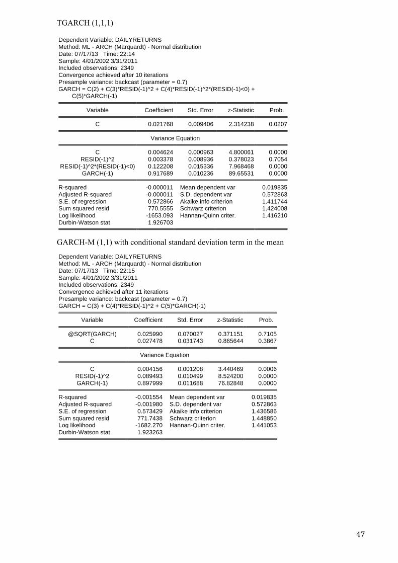
! 47!

TGARCH (1,1,1) !

!


!






! ! ! ! !! ! ! ! !




RESID("1)^2! 0.089493! 0.010499! 8.524200! 0.0000!GARCH("1)! 0.897999! 0.011688! 76.82848! 0.0000!



! ! ! ! !! ! ! ! !

! 48!


!

EGARCH (1,1) !




RESID("1)^2! 0.089574! 0.010502! 8.529350! 0.0000!GARCH("1)! 0.897921! 0.011690! 76.81001! 0.0000!



! ! ! ! !! ! ! ! !



C(3)! 0.112926! 0.014785! 7.637921! 0.0000!C(4)! "0.089265! 0.009485! "9.411674! 0.0000!C(5)! 0.983190! 0.003324! 295.8149! 0.0000!



! ! ! ! !! ! ! ! !

! 49!

China GARCH (1,1)

!

TGARCH (1,1,1) !

!

Dependent!Variable:!DAILYRETURNS! !Method:!ML!"!ARCH!(Marquardt)!"!Normal!distribution!Date:!07/18/13!!!Time:!15:01! ! !Sample!(adjusted):!1/03/2005!3/31/2011! !Included!observations:!1629!after!adjustments! !Convergence!achieved!after!13!iterations! !Presample!variance:!backcast!(parameter!=!0.7)!GARCH!=!C(2)!+!C(3)*RESID("1)^2!+!C(4)*GARCH("1)!


RESID("1)^2! 0.053578! 0.006478! 8.270552! 0.0000!GARCH("1)! 0.939561! 0.006802! 138.1332! 0.0000!



! ! ! ! !! ! ! ! !

Dependent!Variable:!DAILYRETURNS! !Method:!ML!"!ARCH!(Marquardt)!"!Normal!distribution!Date:!07/18/13!!!Time:!15:02! ! !Sample!(adjusted):!1/03/2005!3/31/2011! !Included!observations:!1629!after!adjustments! !Convergence!achieved!after!14!iterations! !Presample!variance:!backcast!(parameter!=!0.7)!GARCH!=!C(2)!+!C(3)*RESID("1)^2!+!C(4)*RESID("1)^2*(RESID("1)<0)!+!!!!!!!!!C(5)*GARCH("1)! ! !





! ! ! ! !! ! ! ! !

! 50!



!


! ! ! ! !! ! ! ! !Variable! Coefficient! Std.!Error! z"Statistic! Prob.!!!! ! ! ! !! ! ! ! !@SQRT(GARCH)! "0.039905! 0.078664! "0.507290! 0.6120!


RESID("1)^2! 0.053400! 0.006465! 8.259962! 0.0000!GARCH("1)! 0.939856! 0.006766! 138.9062! 0.0000!



! ! ! ! !! ! ! ! !


! ! ! ! !! ! ! ! !Variable! Coefficient! Std.!Error! z"Statistic! Prob.!!!! ! ! ! !! ! ! ! !GARCH! "0.017057! 0.047282! "0.360759! 0.7183!


RESID("1)^2! 0.053441! 0.006472! 8.257545! 0.0000!GARCH("1)! 0.939762! 0.006779! 138.6266! 0.0000!



! ! ! ! !! ! ! ! !

! 51!

EGARCH (1,1) !

!

!!!!!!!!!!!!!!!!!!!!!!!!

Dependent!Variable:!DAILYRETURNS! !Method:!ML!"!ARCH!(Marquardt)!"!Normal!distribution!Date:!07/18/13!!!Time:!15:04! ! !Sample!(adjusted):!1/03/2005!3/31/2011! !Included!observations:!1629!after!adjustments! !Convergence!achieved!after!22!iterations! !Presample!variance:!backcast!(parameter!=!0.7)!LOG(GARCH)!=!C(2)!+!C(3)*ABS(RESID("1)/@SQRT(GARCH("1)))!+!C(4)!!!!!!!!!*RESID("1)/@SQRT(GARCH("1))!+!C(5)*LOG(GARCH("1))!


C(3)! 0.119974! 0.012553! 9.557482! 0.0000!C(4)! "0.003857! 0.006311! "0.611251! 0.5410!C(5)! 0.987821! 0.002696! 366.3351! 0.0000!



! ! ! ! !! ! ! ! !

! 52!

Appendix 4

Histograms and correlograms of standardized residuals GARCH (1,1) Brazil

India

0

50

100

150

200

250

300

350

400

-5 -4 -3 -2 -1 0 1 2 3 4

Series: RESID01Sample 4/01/2002 3/30/2012Observations 2349

Mean -0.026355Median -0.033941Maximum 3.950321Minimum -5.623176Std. Dev. 0.999928Skewness -0.282704Kurtosis 4.054041


0

100

200

300

400

500

600

-4 -3 -2 -1 0 1 2 3 4 5 6 7




! 53!

Russia

0

100

200

300

400

500

600

700

-7 -6 -5 -4 -3 -2 -1 0 1 2 3 4 5

Ser ies: Standardized ResidualsSample 4/01/2002 3/31/2011Observations 2349



! 54!

South Africa

China

0

50

100

150

200

250

300

350

-4 -3 -2 -1 0 1 2 3 4




0

40

80

120

160

200

240

280

-4 -3 -2 -1 0 1 2 3 4 5




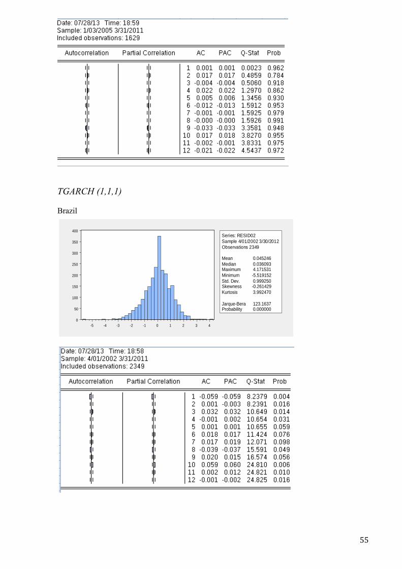
! 55!

TGARCH (1,1,1) Brazil

0

50

100

150

200

250

300

350

400

-5 -4 -3 -2 -1 0 1 2 3 4




! 56!

India

Russia

0

100

200

300

400

500

600

-4 -2 0 2 4 6 8




0

100

200

300

400

500

600

-7 -6 -5 -4 -3 -2 -1 0 1 2 3 4 5




! 57!

South Africa

0

40

80

120

160

200

240

280

320

-4 -3 -2 -1 0 1 2 3




! 58!

China

EGARCH (1,1) Brazil

0

40

80

120

160

200

240

280

-4 -3 -2 -1 0 1 2 3 4 5




0

100

200

300

400

500

600

-6 -5 -4 -3 -2 -1 0 1 2 3 4 5




! 59!

India

0

100

200

300

400

500

600

-4 -2 0 2 4 6 8




! 60!

Russia

South Africa

0

100

200

300

400

500

600

700

-8 -6 -4 -2 0 2 4 6




0

50

100

150

200

250

300

350

-4 -3 -2 -1 0 1 2 3




! 61!

China

0

50

100

150

200

250

300

-5 -4 -3 -2 -1 0 1 2 3 4 5




! 62!

Appendix 5

Dynamic forecasts GARCH (1,1) Brazil India

-2

-1

0

1

2

M4 M5 M6 M7 M8 M9 M10 M11 M12 M1 M2 M3

2011 2012

DAILYRETURF – 2 S.E.

Forecast: DAILYRETURFActual: DAILYRETURNSForecast sample: 4/01/2011 3/30/2012Included observations: 261Root Mean Squared Error 0.673544Mean Absolute Error 0.486456Mean Abs. Percent Error 110.9524Theil Inequality Coefficient 0.933879 Bias Proportion 0.008076 Variance Proportion NA Covariance Proportion NA

.2

.3

.4

.5

.6

M4 M5 M6 M7 M8 M9 M10 M11 M12 M1 M2 M3

2011 2012

Forecast of Variance

-2

-1

0

1

2

M4 M5 M6 M7 M8 M9 M10 M11 M12 M1 M2 M3

2011 2012



.2

.3

.4

.5

.6

.7

M4 M5 M6 M7 M8 M9 M10 M11 M12 M1 M2 M3

2011 2012


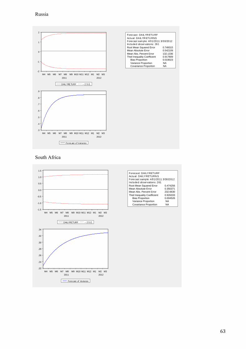
! 63!

Russia South Africa

-2

-1

0

1

2

M4 M5 M6 M7 M8 M9 M10 M11 M12 M1 M2 M3

2011 2012



.3

.4

.5

.6

.7

.8

.9

M4 M5 M6 M7 M8 M9 M10 M11 M12 M1 M2 M3

2011 2012


-1.5

-1.0

-0.5

0.0

0.5

1.0

1.5

M4 M5 M6 M7 M8 M9 M10 M11 M12 M1 M2 M32011 2012



.22

.24

.26

.28

.30

.32

.34

M4 M5 M6 M7 M8 M9 M10 M11 M12 M1 M2 M32011 2012


! 64!

China TGARCH (1,1,1) Brazil

-2

-1

0

1

2

M4 M5 M6 M7 M8 M9 M10 M11 M12 M1 M2 M3

2011 2012



.2

.3

.4

.5

.6

.7

.8

M4 M5 M6 M7 M8 M9 M10 M11 M12 M1 M2 M3

2011 2012


-1.6

-1.2

-0.8

-0.4

0.0

0.4

0.8

1.2

1.6

M4 M5 M6 M7 M8 M9 M10 M11 M12 M1 M2 M32011 2012



.25

.30

.35

.40

.45

.50

.55

M4 M5 M6 M7 M8 M9 M10 M11 M12 M1 M2 M32011 2012


! 65!

India Russia

-1.5

-1.0

-0.5

0.0

0.5

1.0

1.5

M4 M5 M6 M7 M8 M9 M10 M11 M12 M1 M2 M32011 2012



.20

.25

.30

.35

.40

.45

.50

M4 M5 M6 M7 M8 M9 M10 M11 M12 M1 M2 M32011 2012


-2

-1

0

1

2

M4 M5 M6 M7 M8 M9 M10 M11 M12 M1 M2 M3

2011 2012



.3

.4

.5

.6

.7

.8

M4 M5 M6 M7 M8 M9 M10 M11 M12 M1 M2 M3

2011 2012


! 66!

South Africa China

-1.2

-0.8

-0.4

0.0

0.4

0.8

1.2

M4 M5 M6 M7 M8 M9 M10 M11 M12 M1 M2 M32011 2012



.21

.22

.23

.24

.25

.26

M4 M5 M6 M7 M8 M9 M10 M11 M12 M1 M2 M32011 2012


-2

-1

0

1

2

M4 M5 M6 M7 M8 M9 M10 M11 M12 M1 M2 M3

2011 2012



.3

.4

.5

.6

.7

.8

M4 M5 M6 M7 M8 M9 M10 M11 M12 M1 M2 M3

2011 2012


! 67!

EGARCH (1,1)

Brazil India

-2

-1

0

1

2

M4 M5 M6 M7 M8 M9 M10 M11 M12 M1 M2 M3

2011 2012



.2

.3

.4

.5

.6

.7

M4 M5 M6 M7 M8 M9 M10 M11 M12 M1 M2 M3

2011 2012


-1.5

-1.0

-0.5

0.0

0.5

1.0

1.5

M4 M5 M6 M7 M8 M9 M10 M11 M12 M1 M2 M32011 2012



.25

.30

.35

.40

.45

.50

M4 M5 M6 M7 M8 M9 M10 M11 M12 M1 M2 M32011 2012


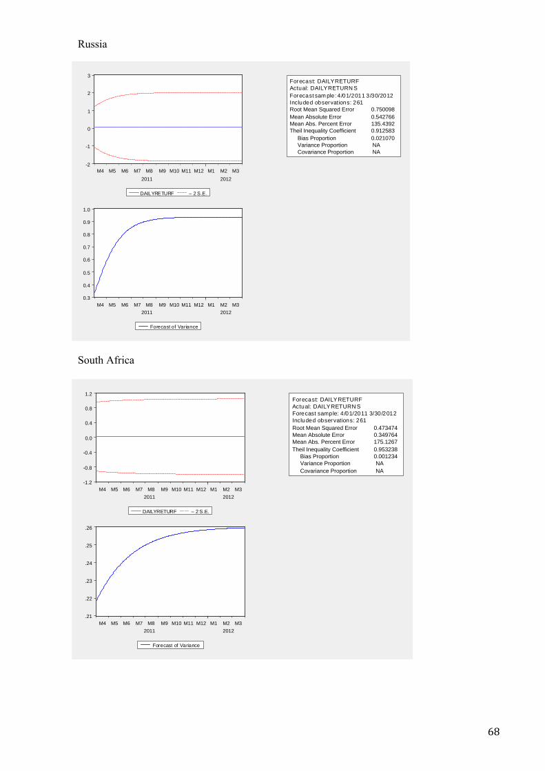
! 68!

Russia South Africa

-2

-1

0

1

2

3

M4 M5 M6 M7 M8 M9 M10 M11 M12 M1 M2 M3

2011 2012



0.3

0.4

0.5

0.6

0.7

0.8

0.9

1.0

M4 M5 M6 M7 M8 M9 M10 M11 M12 M1 M2 M32011 2012


-1.2

-0.8

-0.4

0.0

0.4

0.8

1.2

M4 M5 M6 M7 M8 M9 M10 M11 M12 M1 M2 M32011 2012



.21

.22

.23

.24

.25

.26

M4 M5 M6 M7 M8 M9 M10 M11 M12 M1 M2 M32011 2012


! 69!

China ! !!

-3

-2

-1

0

1

2

3

M4 M5 M6 M7 M8 M9 M10 M11 M12 M1 M2 M3

2011 2012



0.2

0.4

0.6

0.8

1.0

1.2

1.4

M4 M5 M6 M7 M8 M9 M10 M11 M12 M1 M2 M32011 2012


Modelling and Forecasting Volatility of the BRICS Stock Markets: Evidence Using GARCH Models.

Documents

Transcript of Modelling and Forecasting Volatility of the BRICS Stock Markets: Evidence Using GARCH Models.