Introducing VAR and SVAR predictions in system dynamics models

Ann Oper Res (2007) 151:241–267
DOI 10.1007/s10479-006-0118-4
A conditional-SGT-VaR approach with alternativeGARCH models
Turan G. Bali · Panayiotis Theodossiou
Published online: 7 December 2006C© Springer Science + Business Media, LLC 2007
Abstract This paper proposes a conditional technique for the estimation of VaR and expected
shortfall measures based on the skewed generalized t (SGT) distribution. The estimation of
the conditional mean and conditional variance of returns is based on ten popular variations
of the GARCH model. The results indicate that the TS-GARCH and EGARCH models
have the best overall performance. The remaining GARCH specifications, except in a few
cases, produce acceptable results. An unconditional SGT-VaR performs well on an in-sample
evaluation and fails the tests on an out-of-sample evaluation. The latter indicates the need
to incorporate time-varying mean and volatility estimates in the computation of VaR and
expected shortfall measures.
Keywords GARCH models . Skewed generalized t distribution . Conditional value at risk .
Expected shortfall
1 Introduction
Value at Risk (VaR) techniques are widely used to assess the risk exposure of investments.
The VaR for a portfolio is simply an estimate of a specified percentile of the probability
distribution of the portfolio’s returns over a given holding period. The specified percentile
is usually computed for the lower tail of the distribution of returns. For example, a VaR
threshold for the first percentile of daily returns implies that daily loses greater than the VaR
threshold will occur less than 1% of the time.
T. G. Bali (�)Professor of Finance, Department of Economics & Finance, Zicklin School of Business,Baruch College, CUNY, 55 Lexington Avenue, Box B10-225, New York, NY 10010e-mail: Turan [email protected]
P. TheodossiouRutgers University, School of Business,227 Penn Street, Camden, NJ 08102e-mail: [email protected]
Springer

242 Ann Oper Res (2007) 151:241–267
Calculation of portfolio VaR is often based on the variance-covariance approach and
makes the assumption, among other things, that returns follow the normal distribution. Many
researchers show that this assumption is at odds with reality and often leads to misleading VaR
estimates.1 There is substantial empirical evidence showing that the distribution of financial
returns is typically skewed to the left, is peaked around the mean (leptokurtic) and has fat
tails.2 The leptokurtosis is reduced, but not eliminated, when returns are standardized using
time-varying estimates for the means and variances [see Bollerslev, Engle, and Nelson (1994)
and the references therein].
The solutions proposed in the VaR literature to the aforementioned problems are the use of
(a) historical simulation techniques, (b) student’s t , (c) generalized error distribution (GED)
and (d) mixture of two normal distributions. Each of these solutions deals partially with the
issues of skewness and leptokurtosis and cannot fully correct the underestimation of risk
problem.3
This paper proposes a conditional technique for the estimation of VaR measures based on
the skewed generalized t (SGT) distribution of Theodossiou (1998), henceforth called the
conditional-SGT-VaR technique. The SGT provides a flexible tool for modeling the empirical
distribution of financial data exhibiting skewness, leptokurtosis and fat-tails.4 The estimation
of the conditional mean and conditional variance of returns, needed for the implementation
of the technique, is based on several popular variations of the GARCH model. The suitability
of these GARCH models in computing conditional-SGT-VaR measures is also addressed in
the paper.
Although VaR measures constitute a significant advancement over the more traditional
measures mostly based on sensitivities to market variables, their computation can often be a
formidable task in the case of complex portfolios exposed to risks associated with different
risk drivers. Moreover, their computation cannot be split into separate sub-computations
due to the position and risk non-additivity of VaR measures.5 For this reason, Artzner et al.
(1997, 1999) and Delbaen (1998) consider an alternative downside risk measure known as
the “expected shortfall measure.” The latter is simply the conditional expectation of loss of
an investment, given that this loss is beyond the VaR level. This paper also compares the
relative performance of the SGT and normal distributions in constructing expected shortfall
measures of raw and standardized returns.
1 See Longin (2000), McNeil and Frey (2000), Bali (2003), Bali and Neftci (2003), and Seymour and Polakow(2003) among others.2 The fat tails could be attributed to price jumps, the correlations between shocks and changes in volatility,time-varying volatility and other higher order moment dependencies3 Cummins et al. (1990) investigate the use of a four parameter family of probability distributions, the gen-eralized beta of the second kind (GB2), for modeling insurance loss processes, and find that seemingly slightdifferences in modeling the tails can result in large differences in reinsurance premiums and quantiles forthe distribution of total insurance losses. Mittnik and Paolella (2000) and Giot and Laurent (2003) use askewed version of the student-t distribution in calculating VaR. Heikkinen and Kanto (2002) use the symmet-ric student-t density to estimate unconditional value at risk. Jondeau and Rockinger (2003) provide severaleconometric specifications for estimating the conditional volatility, skewness, and kurtosis, which can used tocalculate conditional VaR thresholds.4 The literature on conditional VaR models and their applications to portfolio management is a very large one,e.g., Rockafeller and Uryasev (2000), Krokhmal, Palmquist, and Uryasev (2002), Krokhmal, Uryasev, andZrazhevsky (2002), and Topaloglou, Vladimirou, and Zenios (2002).5 Given a portfolio made of two sub-portfolios, total VaR is not given by the sum of partial VaR’s, with theconsequence that adding a new instrument to a portfolio often make it necessary to re-compute the VaR forthe whole portfolio. For a portfolio depending on multiple risk variables, VaR is not the sum of partial VaR’s.So, for instance, for a convertible bond, VaR is not simply the sum of its interest rate VaR and equity VaR.
Springer

Ann Oper Res (2007) 151:241–267 243
The paper is organized as follows. Section 2 presents discrete time GARCH models.
Section 3 describes the data and presents the estimation results for the GARCH models.
Section 4 presents the Conditional-SGT-VaR approach. Section 5 compares the in-sample
and out-of-sample performance of the conditional-SGT-VaR and conditional-Normal-VaR
measures for the GARCH models. Section 6 provides expected shortfall estimates based on
the SGT and normal distributions. Section 7 concludes the paper.
2 Discrete time GARCH models
Modeling volatility of economic time series has been a popular topic for financial economists
during the past two decades. Engle (1982) developed the Autoregressive Conditional Het-
eroskedasticity (ARCH) model, which was extremely useful in modeling time-varying
volatility of financial data series. Following the introduction of the ARCH model and its
generalization by Bollerslev (1986), there have been numerous refinements of the model
driven by empirical regularities in financial data.6
This paper investigates the suitability of ten variations of the GARCH model in computing
the conditional means and conditional variances for our conditional VaR analysis. The general
form of the GARCH models is as follows:
Rt = α0 + α1 Rt−1 + ut = μt + ut , (1)
g(σt ) = h(σt−1, zt−1, , β0, β1, γ ) + β2g(σt−1,), (2)
g (σt ) = σt , σ2t , or ln (σt ) ,
where μt and σt are the conditional mean and conditional standard deviation of returns Rt
based on the information set �t−1 up to time t−1 and zt = ut /σt .7 The conditional volatility
equations for the various GARCH models are specified as follows:8
AGARCH: Asymmetric GARCH model of Engle (1990)
σ 2t = β0 + β1(γ + σt−1zt−1)2 + β2σ
2t−1, (3)
EGARCH: Exponential GARCH model of Nelson (1991)
ln σ 2t = β0 + β1[|zt−1| − E(|zt−1|)] + β2 ln σ 2
t−1 + γ zt−1, (4)
6 ARCH literature surveys can be found in Bollerslev, Chou, and Kroner (1992), Ding, Granger, and Engle(1993), Bollerslev, Engle, and Nelson (1994), Andersen (1994), Bera, and Higgins (1995), Hentschel (1995),Pagan (1996), Duan (1997), and Bali (2000).7 For simplicity of exposition, we only present GARCH of first order (single-lag) models for both the condi-tional mean and conditional variance specifications. However, in the estimation we considered higher ordermodels as well and explored the possibility of GARCH-in-mean effects.8 One can define the ARCH processes based on the error term, ut , without decomposing ut into standardizedshock, zt , and the conditional volatility, σt . For example, the symmetric GARCH model of Bollerslev (1986)in Eq. (5) can simply be written as σ 2
t = β0 + β1u2t−1 + β2σ
2t−1.
Springer

244 Ann Oper Res (2007) 151:241–267
GARCH: Linear symmetric GARCH model of Bollerslev (1986)
σ 2t = β0 + β1σ
2t−1z2
t−1 + β2σ2t−1, (5)
GJR-GARCH: Threshold GARCH model of Glosten, Jagannathan, and Runkle (1993)
σ 2t = β0 + β1σ
2t−1z2
t−1 + β2σ2t−1 + γ S−
t−1σ2t−1z2
t−1
S−t−1 = 1 for σt−1zt−1 < 0 and S−
t−1 = 0 otherwise, (6)
IGARCH: Integrated GARCH model of Engle and Bollerslev (1986)
σ 2t = β0 + (1 − β2)σ 2
t−1z2t−1 + β2σ
2t−1, (7)
NGARCH: Nonlinear asymmetric GARCH model of Engle and Ng (1993)
σ 2t = β0 + β1σ
2t−1(γ + zt−1)2 + β2σ
2t−1, (8)
QGARCH: Quadratic GARCH model of Sentana (1995)9
σ 2t = β0 + β1σ
2t−1z2
t−1 + β2σ2t−1 + γ σt−1zt−1, (9)
SQR-GARCH: Square-Root GARCH model of Heston and Nandi (1999)10
σ 2t = β0 + β1(γ σt−1 + zt−1)2 + β2σ
2t−1, (10)
TGARCH: Threshold GARCH model of Zakoian (1994)
σt = β0 + β1σt−1|zt−1| + β2σt−1 + γ S−t−1σt−1zt−1
S−t−1 = 1 for σt−1zt−1 < 0 and S−
t−1 = 0 otherwise, (11)
TS-GARCH: The specification proposed by Taylor (1986) and Schwert (1989)
σt = β0 + β1σt−1|zt−1| + β2σt−1, (12)
VGARCH: A version proposed in Engle and Ng (1993)
σ 2t = β0 + β1(γ + zt−1)2 + β2σ
2t−1, (13)
where β0 > 0, 0 ≤ β1 < 1, 0 ≤ β2 < 1 and γ < 0. The conditional volatility parameter γ
allows for asymmetric volatility response to past positive and negative information shocks.
9 In the QGARCH (1,1) model, σ 2t = β0 + β1σ
2t−1z2
t−1 + β2σ2t−1 + γ σt−1zt−1 , positivity of the variance
is achieved when β1, β2 ≥ 0 and γ ≤ 4β0 β1 [Sentana (1995, p. 652)]. To impose these restrictions, one canestimate the likelihood function with the AGARCH model σ 2
t = ρ20 + ρ2
1 (σt−1zt−1 − κ)2 + ρ22σ 2
t−1 , where
β0 = ρ20 + ρ2
1κ2, β1 = ρ21 , β2 = ρ2
2 , and γ = −2ρ21κ . Since both QGARCH and AGARCH models give the
same conditional volatility and VaR estimates, we do not report results from the QGARCH specification.10 Equation (10) converges in the limit to the stochastic variance process of Cox, Ingersoll, and Ross (1985).
Springer
Ann Oper Res (2007) 151:241–267 245
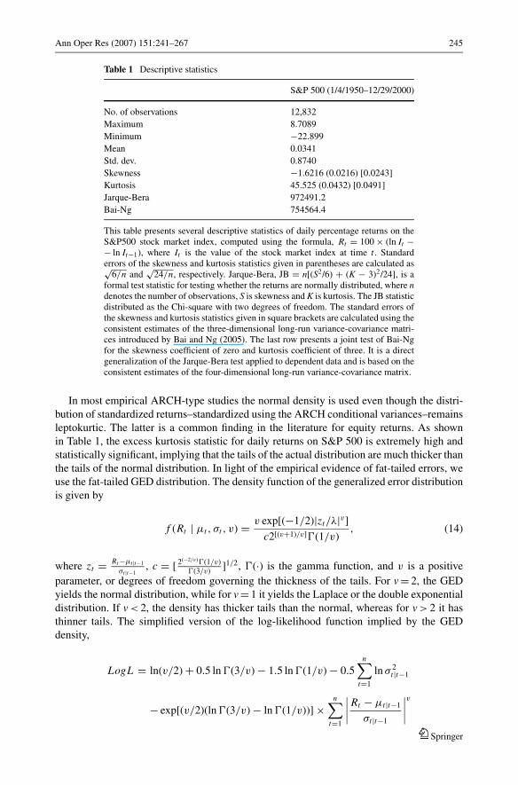
Table 1 Descriptive statistics
S&P 500 (1/4/1950–12/29/2000)
No. of observations 12,832
Maximum 8.7089
Minimum −22.899
Mean 0.0341
Std. dev. 0.8740
Skewness −1.6216 (0.0216) [0.0243]
Kurtosis 45.525 (0.0432) [0.0491]
Jarque-Bera 972491.2
Bai-Ng 754564.4
This table presents several descriptive statistics of daily percentage returns on theS&P500 stock market index, computed using the formula, Rt = 100 × (ln It −− ln It−1), where It is the value of the stock market index at time t . Standarderrors of the skewness and kurtosis statistics given in parentheses are calculated as√
6/n and√
24/n, respectively. Jarque-Bera, JB = n[(S2/6) + (K − 3)2/24], is aformal test statistic for testing whether the returns are normally distributed, where ndenotes the number of observations, S is skewness and K is kurtosis. The JB statisticdistributed as the Chi-square with two degrees of freedom. The standard errors ofthe skewness and kurtosis statistics given in square brackets are calculated using theconsistent estimates of the three-dimensional long-run variance-covariance matri-ces introduced by Bai and Ng (2005). The last row presents a joint test of Bai-Ngfor the skewness coefficient of zero and kurtosis coefficient of three. It is a directgeneralization of the Jarque-Bera test applied to dependent data and is based on theconsistent estimates of the four-dimensional long-run variance-covariance matrix.
In most empirical ARCH-type studies the normal density is used even though the distri-
bution of standardized returns–standardized using the ARCH conditional variances–remains
leptokurtic. The latter is a common finding in the literature for equity returns. As shown
in Table 1, the excess kurtosis statistic for daily returns on S&P 500 is extremely high and
statistically significant, implying that the tails of the actual distribution are much thicker than
the tails of the normal distribution. In light of the empirical evidence of fat-tailed errors, we
use the fat-tailed GED distribution. The density function of the generalized error distribution
is given by
f (Rt | μt , σt , v) = v exp[(−1/2)|zt/λ|v]
c2[(v+1)/v](1/v), (14)
where zt = Rt −μt |t−1
σt |t−1, c = [ 2(−2/v)(1/v)
(3/v)]1/2, (·) is the gamma function, and v is a positive
parameter, or degrees of freedom governing the thickness of the tails. For v = 2, the GED
yields the normal distribution, while for v = 1 it yields the Laplace or the double exponential
distribution. If v < 2, the density has thicker tails than the normal, whereas for v > 2 it has
thinner tails. The simplified version of the log-likelihood function implied by the GED
density,
LogL = ln(v/2) + 0.5 ln (3/v) − 1.5 ln (1/v) − 0.5n∑
t=1
ln σ 2t |t−1
− exp[(v/2)(ln (3/v) − ln (1/v))] ×n∑
t=1
∣∣∣∣ Rt − μt |t−1
σt |t−1
∣∣∣∣vSpringer

246 Ann Oper Res (2007) 151:241–267
yields parameter estimates which are not excessively influenced by extreme observations
that occur with low probability. In addition, the standard errors of the estimated parameters
are robust, allowing for more reliable statistical inference. Another advantage of using the
fat-tailed GED distribution is that one can formally test the empirical validity of existing
models that assume normality.
3 Data and estimation results
The data consist of daily returns on the S&P500 composite index from 1/4/1950 to 12/29/2000
(12832 observations). The computation of the index returns (Rt ) is based on the formula,
Rt = ln(It ) − ln(It−1), where It is the value of the stock market index for period t.11
Table 1 presents several preliminary statistics for the data. The unconditional mean of daily
log-returns is 0.0341% with a standard deviation of 0.87%. The maximum and minimum
values are 8.71% and −22.90%, respectively. The skewness statistic is negative and statis-
tically significant at the 1% level implying that the distribution of daily S&P500 returns is
skewed to the left. The excess kurtosis statistic is very large and significant at the 1% level,
implying that the distribution of returns has much ticker tails than the normal distribution.
Similarly, the Jarque-Bera statistic is also very large and statistically significant, rejecting
the assumption of normality.12
Next we use the Bai and Ng (2005) test for the joint hypothesis that the skewness and
kurtosis coefficients are respectively zero and three. The latter test is a direct generalization
of the aforementioned Jarque-Bera test for data that are serially correlated.13 The Bai and Ng
test statistics, reported in Table 1, reject the null hypothesis at the 1% level of significance.
Panels A and B of Table 2 present the maximum likelihood estimates for the symmetric
and asymmetric GARCH models based on the generalized error and the normal distributions.
The parameters in the conditional mean and conditional variance equations are all statistically
significant at the 1% level. The estimation results reveal the presence of strong conditional
volatility in the S&P500 return series. For example, the symmetric GARCH parameters, β1
and β2, are found to be highly significant and the sum β1 + β2 is close to one. This implies
the existence of strong volatility persistence in stock market returns.
As discussed earlier, for the tail thickness parameter v = 2, the GED density equals the
standard normal density. However, the estimates of v turn out to be highly significant and
less than two for each GARCH model specification. As shown in Panel A of Table 2, the
estimated values for the degrees of freedom parameter v, range between 1.24 and 1.34. A
11 We also examined the DJIA, NASDAQ composite and NYSE stock market indices. Because the qualitativeresults were similar, we present the results for the S&P500 index only. Results on these indices are availableupon request.12 De Ceuster and Trappers (1992) and Peiro (1999) show that the standard test of skewness is not appropriatewhen the series is fat-tailed. For a sample size of 2000 observations, De Ceuster and Trappers (1992) tabulatethat the 95% confidence intervals of the skewness of Student-t distributed observations with a kurtosis of3.5 and 18 are respectively (–0.131; 0.127) and (–0.814; 0.787), i.e., the higher the kurtosis, the larger theconfidence bands of the skewness. Table 3 presents the skewness and kurtosis parameter estimates of SGTand skewed t distributions that give the statistical significance of skewness parameter (λ) after adjusting fortail-thickness of the return distribution.13 Bai and Ng (2005) show that when the data are serially correlated, consistent estimates of three-dimensionallong-run covariance matrices are needed for testing skewness and kurtosis. In the special case of normality,they introduce a joint test for the skewness coefficient of zero and kurtosis coefficient of three based on thefour-dimensional long-run covariance matrix.
Springer

Ann Oper Res (2007) 151:241–267 247
Tabl
e2
Max
imu
mli
kel
iho
od
esti
mat
eso
fth
eG
AR
CH
mo
del
sw
ith
GE
Dan
dn
orm
ald
ensi
ty
Mo
del
sα
0α
1β
0β
1β
2γ
VL
og-L
LR
Pan
elA
.G
ener
aliz
eder
ror
dis
trib
uti
on
AG
AR
CH
0.0
00
34
0.1
23
60
.00
00
00
40
.08
51
0.8
96
9−0
.00
34
41
.33
62
44
87
4.5
01
30
.88
(6.1
72
6)
(14
.42
0)
(2.8
07
6)
(18
.24
7)
(19
6.7
7)
(−1
1.2
68
)(−
50
.62
2)
EG
AR
CH
0.0
00
36
0.1
25
1−0
.35
72
0.1
83
30
.96
24
−0.0
56
71
.24
12
44
87
1.8
31
12
.55
(6.8
47
5)
(15
.59
8)
(−9
.85
20
)(3
1.7
63
)(2
60
.30
)(−
9.9
06
9)
(−5
3.1
75
)
GA
RC
H0
.00
04
70
.12
07
0.0
00
00
10
0.0
86
10
.90
32
0.0
1.3
21
94
48
09
.06
Sy
mm
etri
c
(8.7
48
2)
(14
.23
0)
(8.9
17
9)
(18
.96
7)
(18
8.8
9)
(−5
0.5
06
)
GJR
GA
RC
H0
.00
03
70
.12
43
0.0
00
00
11
0.0
42
30
.89
89
−0.0
90
51
.33
75
44
86
3.6
61
09
.20
(6.8
96
7)
(14
.53
2)
(10
.09
5)
(8.4
39
4)
(19
0.6
5)
(−1
1.7
73
)(−
49
.73
6)
NG
AR
CH
0.0
00
33
0.1
24
80
.00
00
01
10
.08
13
0.8
77
1−0
.60
09
1.3
44
74
48
95
.14
17
0.1
6
(6.0
47
7)
(14
.59
2)
(10
.48
6)
(17
.11
5)
(16
6.8
5)
(−1
1.4
74
)(−
50
.01
9)
SQ
RG
AR
CH
0.0
00
23
0.1
27
50
.00
00
00
30
.00
00
04
0.8
83
9−1
16
.69
1.3
17
54
47
89
.88
21
0.6
8
(4.1
51
2)
(15
.31
7)
(5.9
15
3)
(14
.10
2)
(14
9.5
8)
(−1
3.3
40
)(−
53
.56
4)
TG
AR
CH
0.0
00
34
0.1
28
40
.00
02
72
0.1
54
40
.88
53
−0.0
95
91
.31
54
44
84
5.7
71
52
.04
(6.3
14
0)
(16
.68
8)
(23
.62
5)
(26
.68
3)
(24
6.8
3)
(−1
5.0
67
)(−
50
.71
3)
TS
GA
RC
H0
.00
04
90
.12
66
0.0
00
23
80
.11
15
0.8
86
40
.01
.29
66
44
76
9.7
5S
ym
met
ric
(9.4
78
7)
(16
.54
9)
(22
.51
6)
(24
.91
3)
(23
9.1
9)
(−5
1.2
64
)
VG
AR
CH
0.0
00
20
0.1
26
10
.00
00
00
10
.00
00
04
0.9
35
5−0
.74
78
1.3
11
74
47
80
.17
19
1.2
6
(3.5
94
8)
(15
.15
6)
(9.4
18
3)
(15
.16
5)
(25
1.8
9)
(−1
8.7
83
)(−
54
.76
7)
(Con
tinu
edon
next
page
.)
Springer

248 Ann Oper Res (2007) 151:241–267
Tabl
e2
(Con
tinu
ed).
Mo
del
sα
0α
1β
0β
1β
2γ
Log
-LL
R
Pan
elB
.N
orm
ald
istr
ibu
tio
n
AG
AR
CH
0.0
00
25
0.1
41
10
.00
00
00
90
.09
49
0.8
83
4−0
.00
30
24
44
89
.32
14
7.3
0
(3.9
79
0)
(15
.02
4)
(13
.64
4)
(41
.88
7)
(33
7.7
0)
(−2
1.4
10
)
EG
AR
CH
0.0
00
25
0.1
34
1−0
.38
97
0.1
83
90
.97
42
−0.0
64
34
45
13
.67
31
2.4
9
(4.2
91
9)
(15
.02
9)
(−2
8.8
89
)(5
7.2
06
)(7
68
.96
)(−
30
.59
4)
GA
RC
H0
.00
04
30
.13
71
0.0
00
00
14
0.0
97
50
.88
83
0.0
44
41
5.6
7S
ym
met
ric
(8.1
37
7)
(14
.98
8)
(19
.83
1)
(47
.06
8)
(34
1.9
4)
GJR
GA
RC
H0
.00
02
80
.14
09
0.0
00
00
15
0.0
49
50
.88
66
−0.0
91
94
44
87
.95
14
4.5
6
(4.8
42
6)
(15
.27
8)
(22
.32
6)
(16
.38
0)
(31
5.8
1)
(−2
2.6
08
)
NG
AR
CH
0.0
00
22
0.1
43
10
.00
00
01
50
.08
97
0.8
67
1−0
.54
90
44
52
4.1
82
17
.02
(3.6
47
6)
(15
.42
1)
(23
.12
6)
(34
.89
0)
(30
1.6
0)
(−2
0.6
19
)
SQ
RG
AR
CH
0.0
00
09
0.1
54
00
.00
00
00
30
.00
00
05
0.8
78
4−1
08
.41
44
37
7.6
13
08
.16
(1.5
10
3)
(17
.53
6)
(8.7
48
6)
(36
.98
1)
(38
6.6
0)
(−3
0.5
65
)
TG
AR
CH
0.0
00
26
0.1
52
20
.00
03
88
0.1
73
50
.85
81
−0.0
98
34
44
33
.02
19
2.2
2
(4.7
61
1)
(22
.71
9)
(39
.56
8)
(64
.62
9)
(41
6.2
6)
(−2
9.3
87
)
TS
GA
RC
H0
.00
05
00
.15
50
0.0
00
34
20
.13
27
0.8
58
30
.04
43
36
.91
Sy
mm
etri
c
(9.9
42
8)
(23
.16
0)
(36
.51
0)
(70
.95
2)
(40
4.7
1)
VG
AR
CH
0.0
00
05
0.1
48
20
.00
00
00
10
.00
00
05
0.9
27
4−0
.64
52
44
35
3.0
62
59
.06
(0.8
66
0)
(16
.65
3)
(10
.78
2)
(44
.89
6)
(45
7.6
2)
(−3
7.2
51
)
Pan
elA
and
Bp
rese
nt
the
max
imu
mli
kel
iho
od
esti
mat
eso
fth
eG
AR
CH
mo
del
sw
ith
GE
Dan
dN
orm
ald
ensi
ty.T
he
asy
mp
toti
ct-
stat
isti
csar
esh
own
inp
aren
thes
es.T
he
t-st
atis
tics
fro
mte
stin
gw
het
her
v=
2(i
.e.,
wh
eth
erth
ere
turn
sfo
llow
an
orm
ald
istr
ibu
tio
n)
are
giv
enin
par
enth
eses
un
der
v.L
og-L
isth
em
axim
ized
log
-lik
elih
oo
dva
lue.
LR
isth
elo
g-l
ikel
ihood
rati
ote
stst
atis
tics
for
the
null
hypoth
esis
of
sym
met
ric
GA
RC
Hm
odel
s,i.
e.,γ
=0
.
Springer

Ann Oper Res (2007) 151:241–267 249
comparison of the maximized log-likelihood values of the GED and normal log-likelihood
specifications for each GARCH model indicates that v is statistically different from two. The
latter implies that the distribution of daily (standardized) returns is leptokurtic relative to the
normal distribution. Moreover, the results suggest that the double exponential or Laplace
with v = 1 is a more appropriate than the normal density function. An intuitive understanding
can be gained by realizing that for the normal distribution (v = 2) the degree of kurtosis is
equal to 3, while for the double exponential or Laplace distribution (v = 1) the degree of
kurtosis is equal to 6.
A notable point in Table 2 is that the asymmetry parameter γ of the conditional volatility
equations is highly significant. This parameter allows for an asymmetric volatility response
in the diffusion function to past positive and negative information shocks. It is found to be
negative for all volatility models implying that negative shocks exert larger impact on stock
market volatility than positive shocks of the same magnitude. This finding may be the result
of the leverage or the initial margin requirements, e.g., Hardouvelis and Theodossiou (2002).
The presence of asymmetry in return volatility is further evaluated using a likelihood ratio
(LR) based on the sample log-likelihood functions of the asymmetric and symmetric GARCH
models. Specifically, LR = −2(LogL∗–LogL), where LogL
∗and LogL are respectively the
maximized log-likelihood values under the null hypothesis of γ = 0 and the alternative
hypothesis of γ 0. The LR statistic follows the χ2(1) distribution with one degree of freedom.
The LR statistics in Table 2 are well above the critical value, reconfirming the presence of
asymmetric volatility in the return series.
4 A conditional value at risk approach
The discrete time version of the geometric Brownian motion governing financial price move-
ments is:
Rt = ln (Pt+�t ) − ln (Pt ) = μ∗�t + zσ ∗√�t, (15)
where μ∗ and σ ∗ are the annualized mean and standard deviation of Rt , �t is the length of time
between two successive prices and �Wt = z√
�t is a discrete approximation of the Wiener
process. The latter term has mean zero, variance �t and follows the normal distribution.14
In the case of time-varying mean and variance, the above equation can be modified to reflect
these dependencies as:
Rt = μ∗t �t + zσ ∗
t
√�t, (16)
where μ∗t and σ ∗
t are annualized measures of conditional mean and conditional standard
deviation of the log-return Rt . This paper employs daily data, thus the length of time �treflects that of a trading day and is approximately equal to 1/252. For simplicity, the above
equation can be rewritten as
Rt = μt + zσt , (17)
14 The method presented here can also be applied to profits and losses generated by portfolios of financialassets.
Springer
250 Ann Oper Res (2007) 151:241–267
where μt = μ∗t �t and σt = σ ∗
t
√�t are respectively the conditional mean and conditional
standard deviation of daily returns. Note that the standardized return z = (Rt −μt )/σ t pre-
serves the properties of zero mean and unit variance.
There is substantial empirical evidence showing that the distributions of returns of fi-
nancial assets are typically skewed to the left and peaked around the mode and, have fat
tails. The fat tails suggest that extreme outcomes happen much more frequently than would
be predicted by the normal distribution. Similarly, the distribution of standardized returns,
although normalized, follows a similar pattern.
The conditional threshold for Rt at a given coverage probabilityø, denoted by θ t , is obtained
from the solution of the following cumulative distribution of returns,
Pr(Rt ≤ θt | �t−1) ≡∫ θt
−∞f (Rt | �t−1)d Rt = φ, (18)
where Pr(·) denotes the probability and f (Rt | �t−1) is the conditional probability density
function for Rt .
The above probability function can be written in terms of the standardized returns as
follows:
Pr (Rt ≤ θt | �t−1) = Pr
(Rt − μt
σt≤ θt − μt
σt
∣∣∣∣ �t−1
)= Pr
(z ≤ a = θt − μt
σt
)=
∫ a
−∞f (z) dz = φ, (19)
where the density f(z) and the threshold a associated with the coverage probability φ do not
depend on the information set �t−1. The latter is a byproduct of the assumption that the series
of standardized returns z is identically and independently distributed. The latter assumption
is consistent with empirical evidence related to the GARCH models for stock returns.
The skewed generalized t (SGT) probability density function for the standardized residuals
is:
f = C
(1 + |z + δ|k
((n + 1) | k)(1 + sign(z + δ)λ)kθ k
)− n+1k
(20)
where
C = .5 k
(n + 1
k
)− 1k
B
(n
k,
1
k
)−1
θ−1,
θ = 1/√
g − ρ2,
δ = ρθ,
ρ = 2λB
(n
k,
1
k
)−1 (n + 1
k
) 1k
B
(n − 1
k,
2
k
),
Springer

Ann Oper Res (2007) 151:241–267 251
Table 3 Maximum likelihood estimates of alternative distribution functions
Distribution μ σ λ k N Log-L
SGT 0.00036 0.008501 −0.02455 1.60084 5.2113 43948.62
(4.8204)∗∗ (86.631)∗∗ (−2.2302)∗ (26.421)∗∗ (12.791)∗∗
Generalized t 0.00045 0.00853 0 1.62115 5.0227 43948.21
(7.2617)∗∗ (83.557)∗∗ (26.168)∗∗ (13.063)∗∗
Skewed t 0.00099 0.00875 −0.02647 2 3.6890 43938.56
(3.7824)∗∗ (60.960)∗∗ (−2.1958)∗ (27.569)∗∗
Symmetirc t 0.00044 0.00875 0 2 3.6889 43936.32
(7.0147)∗∗ (61.074)∗∗ (27.608)∗∗
Normal 0.00034 0.00874 0 2 ——- 42611.27
(4.2735)∗∗ (733.25)∗∗
This table presents the parameter estimates of the SGT, Generalized t , Skewed t , Symmetric t , and Normaldistributions. The results are based on the daily raw returns on the S&P 500 composite index spanning theperiod 1/4/1950–12/29/2000 (12832 observations). Asymptotic t−statistics are given in parentheses. Log-L isthe maximized log-likelihood value. ∗,∗∗ denote significance at the 5% and 1% level, respectively.
and
g = (1 + 3λ2
)B
(n
k,
1
k
)−1 (n + 1
k
) 2k
B
(n − 2
k,
3
k
).
λ is a skewness parameter obeying the constraint |λ| < 1, n and k are positive kurtosis
parameters, sign is the sign function, B(·) is the beta function and δ is the Pearson’s skewness
and mode of f(z). The SGT parameters are obtained from the maximization of the sample
log-likelihood function
L =T∑
t=1
ln f (zt | n, k, λ), (21)
with respect to n, k, and λ; see Theodossiou (1998) for the estimation details.
The SGT nests several well-known distributions. Specifically, it gives for λ = 0 the
generalized-t of McDonald and Newey (1988), for k = 2 the skewed t of Hansen (1994),
for n = ∞ the skewed generalized error distribution, for n = ∞ and λ = 0 the generalized
error distribution or power exponential distribution of Subbotin (1923) [used by Box and
Tiao (1962) and Nelson (1991)], for n = ∞, λ = 0 and k = 1 the Laplace or double expo-
nential distribution, for n = ∞, λ = 0 and k = 2 the normal distribution and for n = ∞, λ = 0
and k = ∞ the uniform distribution [see Hansen, McDonald, and Theodossiou (2001) for a
comprehensive survey on the skewed fat-tailed distributions].
Table 3 presents the parameter estimates of the SGT of Theodossiou (1998), the gener-
alized t of McDonald and Newey (1988), the skewed t of Hansen (1994), the symmetric
standardized t of Bollerslev (1987), and the normal distribution. The LR test results indicate
rejection of the skewed t , symmetric t and normal distributions in favor of the SGT. The gen-
eralized t of McDonald and Newey cannot be rejected based on the maximized log-likelihood
values.15
15 For the SGT and normal distributions, we calculated the Kolmogorov-Smirnov (KS) statistic for testing thenull hypothesis that the data follow the corresponding distribution function. The KS statistic of 0.06393 for
Springer

252 Ann Oper Res (2007) 151:241–267
Table 4 presents the estimated SGT parameters for the standardized returns of the GARCH
models. Observe that in all cases, the parameter n is close to six indicating significant fat tails
for the empirical distribution of standardized returns. The parameter k has values close to those
of the normal distribution (i.e., two) indicating no peakness for the empirical distribution.
The skewness parameter is negative and statistically significant for all models indicating that
the distribution of standardized returns is skewed to the left. The LR-Normal ratio for testing
the null hypothesis of normality of standardized returns against that of the SGT is large and
highly significant rejecting the null hypothesis of normality.
Given the probability density function of standardized returns f(z), the threshold a can be
easily obtained from the solution of the equation
∫ a
−∞f (z) dz = φ. (22)
That is, by finding the numerical value of a that equalizes the area under f(z) to the coverage
probability φ . In the case of traditional VaR analysis (normal distribution), the value of the
threshold for φ = 1% is constant and equal a = −2.326.16 However, in the more general case
of the SGT, the value of a is a function of the skewness and kurtosis parameters λ, k and n.
Given the estimated threshold a, the conditional (time-varying) threshold for the returns
can be computed using the equation
θt = μt + aσt , (23)
where the values of μt and σ t are based on anyone of the AR(1)-GARCH models presented
previously. This equation is used to compute the conditional 1-day VaR thresholds and
evaluate the performance and suitability of the GARCH models, considered in the paper, and
the conditional-SGT-VaR technique.17,18
the normal distribution indicates rejection of the null hypothesis at the 1% level, whereas the KS statistic of0.00928 for SGT suggests that the index return data follow the SGT distribution.16 The values of a for the normal distribution associated with the 0.5%, 1%, 1.5%, 2%, 2.5%, and 5% VaRtails are 2.5758, 2.326, 2.1701, 2.0536, 1.960, and 1.645, respectively.17 We should note that the conditional mean-volatility models given in Eqs. (1)–(13) are estimated in a firststep and the tail distributions in a second step because of the absence of SGT-GARCH computer programs.Currently, we do not have the estimation technology for SGT-GARCH models. However, to check the ro-bustness of our findings, we use alternative distributions in the first step estimation. For example, our tablespresent results based on the generalized error distribution (GED). At an earlier stage of the study, we alsouse the skewed generalized error distribution (SGED) of Theodossiou (2001), the generalized t distributionof McDonald and Newey (1988), and the skewed t distribution of Hansen (1994) in the first step estimation.Using the standardized returns obtained from the SGED, generalized t and Skewed t distributions, we calculatethe VaR measures based on the SGT density. The results turn out to be very similar to those reported in ourtables. This indicates that the second step estimation (i.e., estimation of tail distributions) is more crucial toVaR calculations.18 Engle and Manganelli (2004) introduce a conditional autoregressive VaR model based on the quintileregression approach. Wu and Xiao (2002) present a comprehensive analysis of several left-tail measures usingthe ARCH quintile regression approach.
Springer

Ann Oper Res (2007) 151:241–267 253
Tabl
e4
Par
amet
eres
tim
ates
of
the
SG
Td
istr
ibu
tio
nfo
rth
est
and
ard
ized
retu
rns
of
GA
RC
HM
od
els
AG
AR
CH
EG
AR
CH
GA
RC
HG
JRG
AR
CH
NG
AR
CH
SQ
RG
AR
CH
TG
AR
CH
TS
GA
RC
HV
GA
RC
HU
nco
nd
itio
nal
k2
.03
50
2.2
23
61
.95
73
2.0
10
82
.04
98
1.9
71
72
.07
78
1.9
84
01
.97
03
1.6
20
4
(26
.34
)∗∗
(24
.57
)∗∗
(26
.23
)∗∗
(26
.23
)∗∗
(26
.24
)∗∗
(26
.52
)∗∗
(25
.67
)∗∗
(25
.76
)∗∗
(26
.63
)∗∗
(26
.04
)∗∗
λ−0
.03
58
−0.0
26
6−0
.04
19
−0.0
40
5−0
.03
76
−0.0
28
5−0
.03
51
−0.0
37
3−0
.02
80
−0.0
24
7
(−2
.79
)∗∗
(−2
.01
)∗∗
(−3
.34
)∗∗
(−3
.17
)∗∗
(−2
.92
)∗∗
(−2
.26
)∗∗
(−2
.72
)∗∗
(−2
.96
)∗∗
(−2
.22
)∗∗
(−2
.22
)∗∗
n6
.52
23
5.8
19
46
.71
32
6.6
53
26
.54
28
6.6
11
36
.13
16
6.3
54
26
.55
88
5.0
36
0
(13
.59
)∗∗
(14
.21
)∗∗
(12
.44
)∗∗
(13
.08
)∗∗
(13
.56
)∗∗
(13
.01
)∗∗
(13
.99
)∗∗
(12
.78
)∗∗
(13
.19
)∗∗
(12
.94
)∗∗
S−0
.11
30
−0.0
84
7−0
.13
53
−0.1
27
3−0
.11
72
−0.0
92
5−0
.11
47
−0.1
24
5−0
.09
16
−0.1
38
6
K5
.29
31
5.6
02
35
.35
92
5.2
50
25
.23
46
5.3
92
55
.58
78
5.6
18
95
.44
50
12
.07
5
Log
-L−1
78
45
.54
−17
60
8.7
8−1
78
39
.65
−17
85
1.5
7−1
78
54
.07
−17
82
5.2
9−1
77
96
.02
−17
78
3.2
3−1
78
14
.49
−15
13
7.4
3
LR
-GE
D1
76
.86
∗∗2
02
.06
∗∗1
51
.86
∗∗1
67
.46
∗∗1
78
.20
∗∗1
60
.82
∗∗1
85
.78
∗∗1
57
.10
∗∗1
65
.42
∗∗4
56
2.8
2∗∗
LR
-No
rmal
97
0.9
0∗∗
87
1.0
8∗∗
94
6.0
5∗∗
93
4.6
2∗∗
94
0.1
8∗∗
99
2.3
0∗∗
10
11
.48
∗∗9
99
.42
∗∗1
03
1.6
8∗∗
70
71
.58
∗∗
Th
ista
ble
pre
sen
tsth
ep
aram
eter
esti
mat
esfo
rth
esk
ewed
gen
eral
ized
t(S
GT
)d
istr
ibu
tio
nu
sin
gth
est
and
ard
ized
retu
rns
of
allG
AR
CH
mo
del
s.T
he
stan
dar
diz
edre
turn
sar
eo
bta
ined
fro
mth
eG
ED
-AR
(1)-
GA
RC
Hsp
ecifi
cati
on
s.P
aren
thes
esin
clu
de
the
asy
mp
toti
ct-
stat
isti
csfo
rth
ep
aram
eter
so
ffa
t-ta
ils
n,le
pto
ku
rto
sis
kan
dsk
ewn
ess
λ.
San
dK
are
the
esti
mat
edsk
ewn
ess
and
ku
rto
sis
stat
isti
cso
fst
and
ard
ized
retu
rns.
Log
-Lis
the
max
imiz
edlo
g-l
ikel
iho
od
valu
eo
fth
eS
GT
den
sity
.L
R-N
orm
al(L
R-G
ED
)is
the
likel
ihood
rati
ost
atis
tic
from
test
ing
the
null
hypoth
esis
that
the
seri
esfo
llow
the
Norm
al(G
ED
)dis
trib
uti
on
agai
nst
the
SG
Tsp
ecifi
cati
on
.∗,∗
∗d
eno
tesi
gn
ifica
nce
atth
e5
%an
d1
%le
vel
s,re
spec
tivel
y.
Springer

254 Ann Oper Res (2007) 151:241–267
5 Risk measurement performance of conditional VaR models
In this section, we evaluate the in-sample and out-of-sample risk measurement performance
of conditional value at risk models based on the unconditional and conditional coverage test
statistics.
5.1 Evaluation of alternative GARCH-SGT-VaR specifications
Table 5 presents statistics on the VaR thresholds (a) of all models for the coverage probabilities
(φ) 0.5%, 1%, 1.5%, 2%, 2.5% and 5% using the entire sample. Specifically, columns 2 to
10 present statistics for the nine conditional GARCH-SGT-VaR models and the last column
presents the statistics for the unconditional-SGT-VaR model based on the standardized returns
computed using the unconditional model, i.e., constant mean and constant standard deviation
of returns.
The first row for each coverage probability presents the estimated thresholds of the ten
models. The second row presents the actual and expected (in parentheses) number of stan-
dardized returns (observations) that fall below each threshold. The third row presents the
log-likelihood ratio (LR) for testing the null hypothesis that the actual and the expected num-
ber of observations falling below each threshold are statistically the same. This is computed
using the formula
L R = 2[τ ln(τ/(φN )) + (N − τ ) ln((N − τ )/(N − φN ))], (24)
where N is the number of sample observations, φ is the coverage probability, φN is the
expected number andτ is the number of sample observations that falls below the threshold
a.19 Kupiec (1995) indicates that the LR statistic is uniformly the most powerful statistic for
a given sample and has an asymptotic chi-square distribution with one degree of freedom,
χ2(1). 20
For example, at φ = 1% the estimated threshold for the EGARCH standardized returns is
−2.5857. The expected number of observations that falls below the threshold a = −2.5857
is 128.32 (i.e., 1% of 12832 observations) and the actual number of observations is 122. The
LR statistic for evaluating the performance of the EGARCH model at φ = 1% is
L R = 2[122 ln(122/128.32) + (12,832 − 122) ln ((12,832 − 122)/
(12,832 − 128.32))] = 0.3197.
This LR statistic is statistically insignificant and indicates that the expected and actual number
of observations falling below the aforementioned threshold is statistically the same. The latter
implies that the estimated EGARCH-SGT-VaR threshold provides a good assessment of the
risk exposure of a portfolio mimicking the S&P500 index.
The conditional threshold θt could be computed easily from Eq. (23) by substituting the
estimates for the conditional mean and conditional standard deviation of returns. For example,
assuming that the conditional mean is 0.05% and the conditional standard deviation is 1.2%,
the risk exposure of the institution on a single day will be θt = μt +aσ t = 0.05% −2.5857
19 Assuming that the VaR measures are accurate, the variableτ can be modeled as independent draws form abinomial distribution, see Kupiec (1995).20 The critical value of χ2(1) at the 5% level is 3.841 and at the 1% level is 6.635.
Springer

Ann Oper Res (2007) 151:241–267 255
Tabl
e5
In-s
amp
lep
erfo
rman
ceo
fS
GT
dis
trib
uti
on
wit
hal
tern
ativ
eG
AR
CH
mo
del
sfo
rti
me-
vary
ing
VaR
thre
sho
lds
VaR
AG
AR
CH
EG
AR
CH
GA
RC
HG
JRG
AR
CH
NG
AR
CH
SQ
RG
AR
CH
TG
AR
CH
TS
GA
RC
HV
GA
RC
HU
nco
nd
itio
nal
0.5
%−3
.03
83
−3.0
25
6−3
.09
52
−3.0
56
8−3
.03
37
−3.0
31
3−3
.04
37
−3.0
92
9−3
.02
74
−2.8
07
1
N(0
.5%
)6
1(6
4)
57
(64
)6
0(6
4)
59
(64
)6
1(6
4)
56
(64
)5
9(6
4)
63
(64
)5
4(6
4)
55
(64
)
LR
0.1
60
.83
0.2
80
.43
0.1
61
.09
0.4
30
.02
1.7
11
.38
1%
−2.5
90
4−2
.58
57
−2.6
39
0−2
.60
79
−2.5
88
0−2
.58
05
−2.5
87
7−2
.63
09
−2.5
74
8−2
.30
64
N(1
%)
11
2(1
28
)1
22
(12
8)
11
8(1
28
)1
14
(12
8)
11
4(1
28
)1
07
(12
8)
11
7(1
28
)1
20
(12
8)
10
9(1
28
)1
13
(12
8)
LR
2.1
90
.32
0.8
61
.67
1.6
73
.79
1.0
40
.55
3.0
91
.92
1.5
%−2
.33
88
−2.3
41
2−2
.38
23
−2.3
55
2−2
.33
75
−2.3
27
1−2
.33
30
−2.3
72
3−2
.32
06
−2.0
33
8
N(1
.5%
)1
72
(19
2)
18
4(1
92
)1
73
(19
2)
17
0(1
92
)1
79
(19
2)
17
2(1
92
)1
66
(19
2)
18
0(1
92
)1
69
(19
2)
17
8(1
92
)
LR
2.2
90
.38
2.0
72
.77
0.9
82
.29
3.8
7∗
0.8
43
.02
1.1
3
2%
−2.1
63
9−2
.17
23
−2.2
03
7−2
.17
94
−2.1
63
2−2
.15
09
−2.1
56
6−2
.19
29
−2.1
44
0−1
.84
85
N(2
%)
23
4(2
57
)2
53
(25
7)
24
5(2
57
)2
37
(25
7)
23
5(2
57
)2
38
(25
7)
24
5(2
57
)2
43
(25
7)
24
0(2
57
)2
46
(25
7)
LR
2.0
90
.05
0.5
41
.57
1.9
11
.41
0.5
40
.75
1.1
20
.45
2.5
%−2
.02
98
−2.0
43
2−2
.06
67
−2.0
44
6−2
.02
96
−2.0
15
7−2
.02
17
−2.0
55
7−2
.00
86
−1.7
09
1
N(2
.5%
)3
29
(32
1)
31
7(3
21
)3
27
(32
1)
31
9(3
21
)3
19
(32
1)
30
2(3
21
)3
13
(32
1)
32
4(3
21
)3
02
(32
1)
31
9(3
21
)
LR
0.2
20
.05
0.1
20
.01
0.0
11
.15
0.1
90
.03
1.1
50
.01
5%
−1.6
17
7−1
.64
92
−1.6
45
9−1
.62
99
−1.6
18
8−1
.60
09
−1.6
09
2−1
.63
55
−1.5
93
2−1
.29
64
N(5
%)
64
3(6
42
)6
49
(64
2)
64
7(6
42
)6
41
(64
2)
64
7(6
42
)6
54
(64
2)
65
2(6
42
)6
54
(64
2)
66
3(6
42
)6
63
(64
2)
LR
0.0
00
.09
0.0
50
.00
0.0
50
.25
0.1
80
.25
0.7
50
.75
Aver
age
6.5
3%
3.9
5%
5.2
1%
6.4
6%
5.3
9%
9.0
8%
6.4
4%
3.7
2%
9.7
1%
6.8
7%
MA
%E
Th
ista
ble
pre
sen
tsst
atis
tics
on
the
in-s
amp
lep
erfo
rman
ceo
fS
GT
Dis
trib
uti
on
wit
hA
lter
nat
ive
GA
RC
Hm
od
els
for
tim
e-va
ryin
gV
aRth
resh
old
s.T
he
resu
lts
are
bas
edo
nth
est
and
ard
ized
retu
rns
on
S&
P5
00
span
nin
gth
ep
erio
d1
/4/1
95
0to
12
/29
/20
00
(12
83
2o
bse
rvat
ion
s).T
he
firs
tle
vel
of
nu
mb
ers
atea
chro
war
eth
ees
tim
ated
VaR
thre
sho
lds.
Th
ese
con
dle
vel
of
nu
mb
ers
giv
eth
eac
tual
cou
nts
and
the
exp
ecte
dco
un
tsin
par
enth
eses
(or
the
nu
mb
ero
fo
bse
rvat
ion
sfa
llin
gin
the
0.5
%,1
%,1
.5%
,2%
,2.5
%,a
nd
5%
tail
so
fth
ere
turn
dis
trib
uti
on
).T
he
thir
dle
vel
of
nu
mb
ers
are
the
corr
esp
on
din
gli
kel
iho
od
rati
o(L
R)
stat
isti
cs.
Aver
age
MA
%E
isth
eav
erag
em
ean
abso
lute
per
cen
tag
eer
ror
bas
edo
nth
eac
tual
and
exp
ecte
dco
un
ts.
∗,∗∗
den
ote
sig
nifi
can
ceat
the
5%
and
1%
level
s,re
spec
tivel
y.
Springer

256 Ann Oper Res (2007) 151:241–267
(1.2%) = −3.0528%. That is, on 100 million dollars investment the VaR amount would be
about 3.0528 million dollars.
The LR test statistic is embodied in the market risk amendment (MRA), which requires
commercial banks with significant trading activities to set aside capital to cover the market
risk exposure in their trading accounts. Under the MRA, banks report their VaR estimates to
the regulators, who observe when actual portfolio losses exceed these estimates. Rejection
of the null hypothesis implies that computed VaR estimates are not accurate enough.
The last row of Table 5 gives the average mean absolute percentage errors (MA%E) based
on the actual and expected counts. This is computed as:
MA%E = 1
6
6∑i=1
(τi − φi N
φi N
)(25)
where τ i and φi N are the actual and expected number of observations that fall below the
threshold for the coverage probabilities φ i = 0.5%, 1%, 1.5%, 2%, 2.5% and 5% and i = 1,
2, . . . ,6. Equation (25) measures the relative performance of conditional-SGT-VaR measures
for each GARCH model.
According to the LR statistics, all GARCH-SGT and unconditional-SGT models produce
accurate VaR estimates for the aforementioned coverage probabilities (tail probabilities).
The only exception is the VaR estimate for the TGARCH model at the 1.5% tail probability.
Based on the MA%E statistic, the TS-GARCH has the best overall performance, followed
closely by the EGARCH model. The GARCH and NGARCH model also exhibit good per-
formance. Among the ten GARCH models considered, the performance of the VGARCH
and SQRGARCH models is the worst.
Table 6 presents the same statistics based on a rolling-window holdout sample (out-
of-sample) procedure. This is necessary because in practice portfolio managers obtain VaR
estimates based on past data and subsequently use these estimates to assess the risks associated
with current and future movements of their portfolios’ value. Hence, a true assessment of
VaR’s performance should be based on their out-of-sample rather than estimation sample
(in-sample).
To measure the out-of-sample performance of the conditional-SGT-VaR measures, we pro-
ceed as follows: A 10-year rolling sample, starting 1/4/1950, is used to estimate conditional-
SGT-VaR measures and a 1-year holdout sample (year subsequent to the estimation) to
evaluate their performance. Specifically, the first rolling (estimation) sample includes the
returns for the years 1950 to 1959 (2,514 returns) and the first holdout sample includes the
returns for the year 1960. The estimated VaR thresholds (based on rolling sample) are then
used to compute the number of returns in the 1960 holdout sample falling in the 0.5%, 1%,
1.5%, 2%, 2.5%, and 5% tails of each estimated probability distribution. Next, the estimation
sample is rolled forward by removing the returns for the year 1950 and adding the returns for
the year 1960. Consequently, the new holdout sample includes the returns for the year 1961.
The new estimated VaR thresholds are then used to compute the number of returns in the new
holdout sample falling in the aforementioned tails. The procedure continues until the sample
is exhausted. Given that the returns on S&P500 span the period 1/4/1950 to 12/29/2000,
the 10-year rolling estimation procedure yields a total holdout sample of 41 years or 10302
observations.
The results of Table 6 are quite similar to those of Table 5. The only exceptions are the
results for the VGARCH for the coverage probabilities of 2.5% and 5% and the unconditional
VaR at all coverage probabilities. Based on the MA%E statistics, the TS-GARCH has the
Springer

Ann Oper Res (2007) 151:241–267 257
Tabl
e6
Ou
t-o
f-sa
mp
lep
erfo
rman
ceo
fS
GT
dis
trib
uti
on
wit
hal
tern
ativ
eG
AR
CH
mo
del
sfo
rti
me-
vary
ing
VaR
thre
sho
lds
VaR
AG
AR
CH
EG
AR
CH
GA
RC
HG
JRG
AR
CH
NG
AR
CH
SQ
RG
AR
CH
TG
AR
CH
TS
GA
RC
HV
GA
RC
HU
nco
nd
itio
nal
0.5
%−2
.94
75
−2.9
54
6−3
.02
37
−2.9
76
6−2
.94
50
−2.9
11
9−2
.94
47
−3.0
12
2−2
.91
28
−2.6
44
2
N(0
.5%
)4
8(5
1)
55
(51
)4
9(5
1)
46
(51
)4
6(5
1)
56
(51
)5
4(5
1)
53
(51
)5
1(5
1)
67
(51
)
LR
0.2
60
.22
0.1
30
.63
0.6
30
.37
0.1
10
.04
0.0
14
.23
∗
1%
−2.5
26
6−2
.53
51
−2.5
89
2−2
.55
15
−2.5
25
3−2
.49
14
−2.5
18
3−2
.57
46
−2.4
89
8−2
.18
45
N(1
%)
99
(10
3)
10
2(1
03
)1
00
(10
3)
97
(10
3)
10
1(1
03
)1
08
(10
3)
10
1(1
03
)1
04
(10
3)
10
3(1
03
)1
33
(10
3)
LR
0.1
70
.01
0.1
00
.38
0.0
50
.22
0.0
50
.01
0.0
07
.98
∗∗
1.5
%−2
.28
86
−2.3
00
8−2
.34
36
−2.3
11
0−2
.28
79
−2.2
54
0−2
.27
85
−2.3
28
2−2
.25
11
−1.9
33
8
N(1
.5%
)1
46
(15
4)
15
1(1
54
)1
45
(15
4)
15
0(1
54
)1
51
(15
4)
15
9(1
54
)1
41
(15
4)
14
7(1
54
)1
56
(15
4)
20
4(1
54
)
LR
0.5
10
.09
0.6
40
.15
0.0
90
.12
1.2
80
.40
0.0
11
4.4
6∗∗
2%
−2.1
22
4−2
.13
85
−2.1
72
1−2
.14
30
−2.1
22
0−2
.08
83
−2.1
11
5−2
.15
67
−2.0
84
7−1
.76
32
N(2
%)
21
6(2
06
)2
15
(20
6)
20
6(2
06
)2
05
(20
6)
20
8(2
06
)2
38
(20
6)
21
2(2
06
)2
02
(20
6)
23
2(2
06
)2
66
(20
6)
LR
0.4
50
.36
0.0
00
.01
0.0
14
.72
∗0
.16
0.0
93
.13
16
.13
∗∗
2.5
%−1
.99
45
−2.0
14
2−2
.04
03
−2.0
13
7−1
.99
44
−1.9
61
0−1
.98
33
−2.0
25
1−1
.95
69
−1.6
34
7
N(2
.5%
)2
67
(25
7)
26
5(2
57
)2
71
(25
7)
27
0(2
57
)2
66
(25
7)
30
2(2
57
)2
66
(25
7)
26
7(2
57
)2
97
(25
7)
33
7(2
57
)
LR
0.3
20
.20
0.6
70
.57
0.2
67
.32
∗∗0
.26
0.3
25
.79
∗2
2.6
9∗∗
5%
−1.5
99
0−1
.63
27
−1.6
33
2−1
.61
40
−1.5
99
5−1
.56
79
−1.5
88
3−1
.62
01
−1.5
62
4−1
.25
27
N(5
%)
54
9(5
15
)5
41
(51
5)
54
5(5
15
)5
53
(51
5)
54
7(5
15
)5
85
(51
5)
54
7(5
15
)5
46
(51
5)
58
6(5
15
)6
39
(51
5)
LR
2.1
91
.27
1.7
02
.75
1.9
49
.36
∗∗1
.94
1.8
29
.62
∗∗2
8.8
3∗∗
Aver
age
5.0
5%
3.8
8%
3.9
9%
5.1
9%
4.0
6%
10
.76
%4
.82
%3
.55
%7
.21
%2
9.5
5%
MA
%E
Th
ista
ble
pre
sen
tsst
atis
tics
on
the
ou
t-o
f-sa
mp
lep
erfo
rman
ceo
fS
GT
Dis
trib
uti
on
wit
hA
lter
nat
ive
GA
RC
Hm
od
els
for
tim
e-va
ryin
gV
aRth
resh
old
s.T
he
resu
lts
are
bas
edo
nth
est
and
ard
ized
retu
rns
on
S&
P5
00
and
the
tota
lo
ut-
of-
sam
ple
per
iod
1/4
/19
60
to1
2/2
9/2
00
0(1
03
02
ob
serv
atio
ns)
.T
he
firs
tle
vel
of
nu
mb
ers
atea
chro
war
eth
eav
erag
ees
tim
ated
VaR
thre
sho
lds.
Th
ese
con
dle
vel
of
nu
mb
ers
giv
eth
eav
erag
eac
tual
cou
nts
and
the
exp
ecte
dco
un
tsin
par
enth
eses
(or
the
nu
mb
ero
fo
bse
rvat
ion
sfa
llin
gin
the
0.5
%,1
%,1
.5%
,2
%,2
.5%
,an
d5
%ta
ils
of
the
retu
rnd
istr
ibu
tio
n).
Th
eth
ird
level
of
nu
mb
ers
are
the
corr
esp
on
din
gli
kel
iho
od
rati
o(L
R)
stat
isti
cs.A
ver
age
MA
%E
isth
eav
erag
em
ean
abso
lute
per
cen
tag
eer
ror
bas
edo
nth
eac
tual
and
exp
ecte
dco
un
ts.
∗,∗∗
den
ote
sig
nifi
can
ceat
the
5%
and
1%
level
s,re
spec
tivel
y.
Springer

258 Ann Oper Res (2007) 151:241–267
best overall performance, followed very closely by the EGARCH, GARCH and NGARCH
models. Again, the VGARCH and SQRGARCH perform the worst. The fact that the uncon-
ditional VaR model performs poorly is indicative of the need to use VaR models that account
for time-varying mean and standard deviation of returns.
5.2 Evaluation of alternative GARCH-normal-VaR specifications
Table 7 presents statistics on the in-sample performance of Normal distribution with alter-
native GARCH models for estimating time-varying VaR thresholds. Specifically, columns
2 to 10 show statistics for the nine conditional GARCH-Normal-VaR models and the last
column displays the statistics for the Integrated GARCH (IGARCH) specification which is
very close to the RiskMetrics model.
In its most simple form, the RiskMetrics model is equivalent to the IGARCH model with
normally distributed errors, σ 2t = β0 + (1 − β2)σ 2
t−1z2t−1 + β2σ
2t−1, where the intercept β0 is
restricted at zero and the autoregressive parameter β2 is set at a pre-specified value λ and
the coefficient of σ 2t−1z2
t−1 is equal to 1 – λ. In the original RiskMetrics specification, λ is
assumed to be 0.94 for daily data and the error process is assumed to follow a normal density,
ut = σt zt , where zt is i.i.d. N(0,1) and σ 2t is defined as:
σ 2t = (1 − λ)u2
t−1 + λσ 2t−1 (26)
In this paper, we prefer to estimate a slightly generalized version of the RiskMetrics model
and thus do not restrict β0 at zero.
According to the LR statistics in Table 7, all the GARCH models with normal density
produce inaccurate VaR estimates for the 0.5%, 1%, and 1.5% loss probability levels. In
fact, the GARCH and IGARCH models yield acceptably accurate VaR measures only for the
5% loss probability level. Based on the MA%E statistics, the performance of the GARCH-
Normal and IGARCH-Normal (RiskMetrics) models turns out to be worse than the alternative
volatility specifications. The results in Tables 5 and 7 indicate that among the ten GARCH
models considered in the paper, the conditional SGT distribution performs much better than
the conditional Normal distribution.
Table 8 presents the same statistics based on a rolling-window holdout sample (out-of-
sample) procedure. The procedure used to evaluate the performance of conditional-SGT-
VaR measures is utilized to determine the out-of-sample performance of the conditional-
Normal-VaR measures. Specifically, we use a 10-year rolling sample, starting 1/4/1950, to
estimate conditional-SGT-VaR measures and a 1-year holdout sample (year subsequent to
the estimation) to evaluate their performance. The results in Table 8 are quite similar to those
of Table 7. Based on the LR and MA%E statistics, the asymmetric GARCH models have
slightly better performance than the GARCH-Normal and IGARCH-Normal (RiskMetrics)
specifications. However, comparing Tables 6 and 8 provides strong evidence that the out-of-
sample performance of the conditional SGT distribution is superior to the conditional Normal
distribution.
5.3 Conditional coverage test
As discussed by Christoffersen (1998), VaR estimates can be viewed as interval forecasts of
the lower tail of the return distribution. Interval forecasts can be evaluated conditionally and
Springer

Ann Oper Res (2007) 151:241–267 259
Tabl
e7
In-s
amp
lep
erfo
rman
ceo
fn
orm
ald
istr
ibu
tio
nw
ith
alte
rnat
ive
GA
RC
Hm
od
els
for
tim
e-va
ryin
gV
aRth
resh
old
s
VaR
AG
AR
CH
EG
AR
CH
GA
RC
HG
JRG
AR
CH
NG
AR
CH
SQ
RG
AR
CH
TG
AR
CH
TS
GA
RC
HV
GA
RC
HIG
AR
CH
0.5
%−2
.57
40
−2.5
75
7−2
.59
92
−2.5
79
9−2
.57
12
−2.5
51
4−2
.57
36
−2.6
02
7−2
.54
40
−2.5
55
3
N(0
.5%
)1
10
(64
)1
14
(64
)1
25
(64
)1
13
(64
)1
08
(64
)1
05
(64
)1
13
(64
)1
25
(64
)1
04
(64
)1
23
(64
)
LR
27
.10
∗∗3
1.5
9∗∗
45
.36
∗∗3
0.4
4∗∗
24
.97
∗∗2
1.9
1∗∗
30
.44
∗∗4
5.3
6∗∗
20
.92
∗∗4
2.7
1∗∗
1%
−2.3
24
2−2
.32
58
−2.3
49
6−2
.33
02
−2.3
21
5−2
.30
19
−2.3
24
3−2
.35
35
−2.2
94
5−2
.30
99
N(1
%)
16
0(1
28
)1
66
(12
8)
17
6(1
28
)1
66
(12
8)
16
6(1
28
)1
67
(12
8)
17
1(1
28
)1
81
(12
8)
16
2(1
28
)1
77
(12
8)
LR
7.3
4∗∗
10
.24
∗∗1
6.0
5∗∗
10
.24
∗∗1
0.2
4∗∗
10
.77
∗∗1
3.0
0∗∗
19
.39
∗∗8
.25
∗∗1
6.7
0∗∗
1.5
%−2
.16
83
−2.1
69
9−2
.19
37
−2.1
74
3−2
.16
56
−2.1
46
1−2
.16
87
−2.1
98
0−2
.13
53
−2.1
56
8
N(1
.5%
)2
21
(19
2)
22
2(1
92
)2
33
(19
2)
22
7(1
92
)2
22
(19
2)
22
8(1
92
)2
26
(19
2)
23
5(1
92
)2
20
(19
2)
23
4(1
92
)
LR
4.1
0∗
4.3
9∗
8.1
3∗∗
5.9
6∗
4.3
9∗
6.3
0∗
5.6
2∗
8.9
3∗∗
3.8
4∗
8.5
2∗∗
2%
−2.0
51
8−2
.05
33
−2.0
77
3−2
.05
78
−2.0
49
1−2
.02
98
−2.0
52
4−2
.08
18
−2.0
22
5−2
.04
23
N(2
%)
28
9(2
57
)2
85
(25
7)
30
5(2
57
)2
89
(25
7)
28
3(2
57
)2
77
(25
7)
27
9(2
57
)2
93
(25
7)
27
3(2
57
)3
12
(25
7)
LR
4.0
1∗
3.1
08
.79
∗∗4
.01
∗2
.68
1.6
11
.94
5.0
4∗
1.0
51
1.4
3∗∗
2.5
%−1
.95
82
−1.9
59
7−1
.98
37
−1.9
64
2−1
.95
55
−1.9
36
3−1
.95
90
−1.9
88
4−1
.92
90
−1.9
50
3
N(2
.5%
)3
49
(32
1)
34
0(3
21
)3
64
(32
1)
34
7(3
21
)3
45
(32
1)
33
4(3
21
)3
46
(32
1)
34
7(3
21
)3
41
(32
1)
36
1(3
21
)
LR
2.4
81
.16
5.7
4∗
2.1
51
.84
0.5
51
.99
2.1
51
.29
4.9
8∗
5%
−1.6
43
3−1
.64
46
−1.6
68
9−1
.64
93
−1.6
40
5−1
.62
16
−1.6
44
6−1
.67
42
−1.6
14
4−1
.64
09
N(5
%)
59
5(6
42
)5
97
(64
2)
59
7(6
42
)5
94
(64
2)
59
4(6
42
)5
99
(64
2)
59
5(6
42
)6
01
(64
2)
60
6(6
42
)5
96
(64
2)
LR
3.6
33
.32
3.3
23
.79
3.7
93
.03
3.6
32
.75
2.1
13
.48
Aver
age
23
.41
%2
4.5
4%
32
.21
%2
5.4
2%
23
.19
%2
1.9
7%
25
.26
%3
1.2
7%
20
.11
%3
2.2
3%
MA
%E
Th
ista
ble
pre
sen
tsst
atis
tics
on
the
in-s
amp
lep
erfo
rman
ceo
fN
orm
alD
istr
ibu
tio
nw
ith
Alt
ern
ativ
eG
AR
CH
mo
del
sfo
rti
me-
vary
ing
VaR
thre
sho
lds.
Th
ere
sult
sar
eb
ased
on
the
stan
dar
diz
edre
turn
so
nS
&P
50
0sp
ann
ing
the
per
iod
1/4
/19
50
to1
2/2
9/2
00
0(1
28
32
ob
serv
atio
ns)
.T
he
firs
tle
vel
of
nu
mb
ers
atea
chro
war
eth
ees
tim
ated
VaR
thre
sho
lds.
Th
ese
con
dle
vel
of
nu
mb
ers
giv
eth
eac
tual
cou
nts
and
the
exp
ecte
dco
un
tsin
par
enth
eses
(or
the
nu
mb
ero
fo
bse
rvat
ion
sfa
llin
gin
the
0.5
%,1
%,1
.5%
,2%
,2.5
%,a
nd
5%
tail
so
fth
ere
turn
dis
trib
uti
on
).T
he
thir
dle
vel
of
nu
mb
ers
are
the
corr
esp
on
din
gli
kel
iho
od
rati
o(L
R)
stat
isti
cs.
Aver
age
MA
%E
isth
eav
erag
em
ean
abso
lute
per
cen
tag
eer
ror
bas
edo
nth
eac
tual
and
exp
ecte
dco
un
ts.
∗,∗∗
den
ote
sig
nifi
can
ceat
the
5%
and
1%
level
s,re
spec
tivel
y.
Springer

260 Ann Oper Res (2007) 151:241–267
Tabl
e8
Ou
t-o
f-sa
mp
lep
erfo
rman
ceo
fn
orm
ald
istr
ibu
tio
nw
ith
alte
rnat
ive
GA
RC
Hm
od
els
for
tim
e-va
ryin
gV
aRth
resh
old
s
VaR
AG
AR
CH
EG
AR
CH
GA
RC
HG
JRG
AR
CH
NG
AR
CH
SQ
RG
AR
CH
TG
AR
CH
TS
GA
RC
HV
GA
RC
HIG
AR
CH
0.5
%−2
.57
21
−2.5
78
6−2
.60
46
−2.5
84
1−2
.56
88
−2.5
84
0−2
.57
60
−2.6
08
9−2
.57
65
−2.5
54
4
N(0
.5%
)8
3(5
1)
87
(51
)9
0(5
1)
85
(51
)8
2(5
1)
82
(51
)8
8(5
1)
95
(51
)8
4(5
1)
92
(51
)
LR
16
.21
∗∗2
0.2
3∗∗
23
.49
∗∗1
8.1
7∗∗
15
.27
∗∗1
5.2
7∗∗
21
.29
∗∗2
9.3
7∗∗
17
.18
∗∗2
5.7
8∗∗
1%
−2.3
23
0−2
.32
90
−2.3
54
8−2
.33
44
−2.3
19
8−2
.33
18
−2.3
27
0−2
.35
96
−2.3
24
4−2
.30
95
N(1
%)
12
4(1
03
)1
25
(10
3)
13
4(1
03
)1
25
(10
3)
12
7(1
03
)1
25
(10
3)
13
2(1
03
)1
43
(10
3)
12
5(1
03
)1
35
(10
3)
LR
3.9
9∗
4.3
7∗
8.5
0∗∗
4.3
7∗
5.1
7∗
4.3
7∗
7.4
7∗∗
13
.86
∗∗4
.37
∗9
.04
∗∗
1.5
%−2
.16
76
−2.1
73
2−2
.19
90
−2.1
78
6−2
.16
44
−2.1
74
5−2
.17
15
−2.2
04
0−2
.16
70
−2.1
56
7
N(1
.5%
)1
71
(15
4)
17
0(1
54
)1
75
(15
4)
17
2(1
54
)1
71
(15
4)
17
2(1
54
)1
78
(15
4)
17
8(1
54
)1
67
(15
4)
17
3(1
54
)
LR
1.9
91
.47
2.5
81
.88
1.6
71
.88
3.3
83
.38
0.9
62
.10
2%
−2.0
51
4−2
.05
68
−2.0
82
5−2
.06
21
−2.0
48
2−2
.05
68
−2.0
55
4−2
.08
77
−2.0
49
4−2
.04
25
N(2
%)
22
6(2
06
)2
13
(20
6)
23
5(2
06
)2
21
(20
6)
22
0(2
06
)2
17
(20
6)
21
5(2
06
)2
24
(20
6)
21
3(2
06
)2
40
(20
6)
LR
1.8
50
.22
3.8
8∗
1.0
40
.90
0.5
50
.36
1.5
00
.22
5.3
2∗
2.5
%−1
.95
80
−1.9
63
2−1
.98
89
−1.9
68
6−1
.95
49
−1.9
62
3−1
.96
20
−1.9
94
3−1
.95
49
−1.9
50
7
N(2
.5%
)2
74
(25
7)
26
1(2
57
)2
83
(25
7)
27
1(2
57
)2
68
(25
7)
25
9(2
57
)2
69
(25
7)
26
5(2
57
)2
65
(25
7)
28
1(2
57
)
LR
1.0
00
.04
2.4
20
.67
0.4
00
.00
0.4
80
.20
0.2
02
.05
5%
−1.6
43
9−1
.64
84
−1.6
73
9−1
.65
37
−1.6
40
9−1
.64
43
−1.6
48
0−1
.67
99
−1.6
37
0−1
.64
19
N(5
%)
47
6(5
15
)4
75
(51
5)
48
3(5
15
)4
77
(51
5)
47
6(5
15
)4
78
(51
5)
47
2(5
15
)4
75
(51
5)
47
9(5
15
)4
80
(51
5)
LR
3.3
33
.50
2.2
53
.16
3.3
33
.00
4.0
4∗
3.5
02
.84
2.6
9
Aver
age
19
.68
%1
9.1
8%
25
.10
%1
9.9
7%
18
.96
%1
7.8
6%
22
.28
%2
6.7
2%
18
.00
%2
6.0
7%
MA
%E
Th
ista
ble
pre
sen
tsst
atis
tics
on
the
ou
t-o
f-sa
mp
lep
erfo
rman
ceo
fN
orm
alD
istr
ibu
tio
nw
ith
Alt
ern
ativ
eG
AR
CH
mo
del
sfo
rti
me-
vary
ing
VaR
thre
sho
lds.
Th
ere
sult
sar
eb
ased
on
the
stan
dar
diz
edre
turn
so
nS
&P
50
0an
dth
eto
tal
ou
t-o
f-sa
mp
lep
erio
d1
/4/1
96
0to
12
/29
/20
00
(10
30
2o
bse
rvat
ion
s).
Th
efi
rst
level
of
nu
mb
ers
atea
chro
war
eth
eav
erag
ees
tim
ated
VaR
thre
sho
lds.
Th
ese
con
dle
vel
of
nu
mb
ers
giv
eth
eav
erag
eac
tual
cou
nts
and
the
exp
ecte
dco
un
tsin
par
enth
eses
(or
the
nu
mb
ero
fo
bse
rvat
ion
sfa
llin
gin
the
0.5
%,
1%
,1
.5%
,2
%,
2.5
%,
and
5%
tail
so
fth
ere
turn
dis
trib
uti
on
).T
he
thir
dle
vel
of
nu
mb
ers
are
the
corr
esp
on
din
gli
kel
iho
od
rati
o(L
R)
stat
isti
cs.
Aver
age
MA
%E
isth
eav
erag
em
ean
abso
lute
per
cen
tag
eer
ror
bas
edo
nth
eac
tual
and
exp
ecte
dco
un
ts.
∗,∗∗
den
ote
sig
nifi
can
ceat
the
5%
and
1%
level
s,re
spec
tivel
y.
Springer
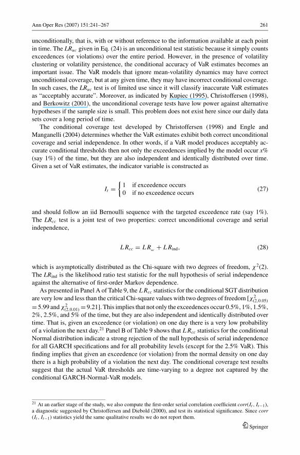
Ann Oper Res (2007) 151:241–267 261
unconditionally, that is, with or without reference to the information available at each point
in time. The LRuc given in Eq. (24) is an unconditional test statistic because it simply counts
exceedences (or violations) over the entire period. However, in the presence of volatility
clustering or volatility persistence, the conditional accuracy of VaR estimates becomes an
important issue. The VaR models that ignore mean-volatility dynamics may have correct
unconditional coverage, but at any given time, they may have incorrect conditional coverage.
In such cases, the LRuc test is of limited use since it will classify inaccurate VaR estimates
as “acceptably accurate”. Moreover, as indicated by Kupiec (1995), Christoffersen (1998),
and Berkowitz (2001), the unconditional coverage tests have low power against alternative
hypotheses if the sample size is small. This problem does not exist here since our daily data
sets cover a long period of time.
The conditional coverage test developed by Christoffersen (1998) and Engle and
Manganelli (2004) determines whether the VaR estimates exhibit both correct unconditional
coverage and serial independence. In other words, if a VaR model produces acceptably ac-
curate conditional thresholds then not only the exceedences implied by the model occur x%
(say 1%) of the time, but they are also independent and identically distributed over time.
Given a set of VaR estimates, the indicator variable is constructed as
It ={
1 if exceedence occurs
0 if no exceedence occurs(27)
and should follow an iid Bernoulli sequence with the targeted exceedence rate (say 1%).
The LRcc test is a joint test of two properties: correct unconditional coverage and serial
independence,
L Rcc = L Ruc + L Rind, (28)
which is asymptotically distributed as the Chi-square with two degrees of freedom, χ2(2).
The LRind is the likelihood ratio test statistic for the null hypothesis of serial independence
against the alternative of first-order Markov dependence.
As presented in Panel A of Table 9, the L Rcc statistics for the conditional SGT distribution
are very low and less than the critical Chi-square values with two degrees of freedom [χ2(2,0.05)
= 5.99 and χ2(2,0.01) = 9.21]. This implies that not only the exceedences occur 0.5%, 1%, 1.5%,
2%, 2.5%, and 5% of the time, but they are also independent and identically distributed over
time. That is, given an exceedence (or violation) on one day there is a very low probability
of a violation the next day.21 Panel B of Table 9 shows that L Rcc statistics for the conditional
Normal distribution indicate a strong rejection of the null hypothesis of serial independence
for all GARCH specifications and for all probability levels (except for the 2.5% VaR). This
finding implies that given an exceedence (or violation) from the normal density on one day
there is a high probability of a violation the next day. The conditional coverage test results
suggest that the actual VaR thresholds are time-varying to a degree not captured by the
conditional GARCH-Normal-VaR models.
21 At an earlier stage of the study, we also compute the first-order serial correlation coefficient corr(It , It−1),a diagnostic suggested by Christoffersen and Diebold (2000), and test its statistical significance. Since corr(It , It−1) statistics yield the same qualitative results we do not report them.
Springer

262 Ann Oper Res (2007) 151:241–267
Tabl
e9
Co
nd
itio
nal
cover
age
test
resu
lts
Per
cen
tile
AG
AR
CH
EG
AR
CH
GA
RC
HG
JRG
AR
CH
NG
AR
CH
SQ
RG
AR
CH
TG
AR
CH
TS
GA
RC
HV
GA
RC
H
Pan
elA
.C
on
dit
ion
alS
GT
dis
trib
uti
on
0.5
%2
.02
2.7
02
.16
2.3
12
.04
2.9
62
.29
1.8
93
.57
1%
2.9
81
.12
1.6
72
.48
2.4
84
.59
1.8
31
.35
3.8
2
1.5
%2
.49
0.5
92
.29
2.9
91
.20
2.5
04
.07
1.0
63
.25
2%
4.2
32
.20
2.7
03
.73
4.0
73
.56
2.6
82
.91
3.2
2
2.5
%3
.79
1.7
62
.26
3.2
93
.63
3.1
22
.24
2.4
72
.82
5%
1.8
21
.92
1.8
91
.84
1.8
92
.08
2.0
12
.04
2.5
7
Pan
elB
.C
on
dit
ion
aln
orm
ald
istr
ibu
tio
n
0.5
%2
7.6
1∗∗
32
.11
∗∗4
5.8
9∗∗
30
.97
∗∗2
5.5
1∗∗
22
.43
∗∗3
0.9
6∗∗
45
.88
∗∗2
1.4
3∗∗
1%
7.4
9∗∗
10
.42
∗∗1
6.2
2∗∗
10
.41
∗∗1
0.4
2∗∗
10
.94
∗∗1
3.1
5∗∗
19
.55
∗∗8
.40
∗∗
1.5
%6
.02
∗∗6
.33
∗∗1
0.0
9∗∗
7.9
1∗∗
6.3
3∗∗
8.2
3∗∗
7.5
4∗∗
10
.86
∗∗5
.76
∗
2%
6.0
5∗∗
5.1
61
0.8
5∗∗
6.0
8∗∗
4.7
33
.66
3.9
97
.07
∗∗3
.08
2.5
%2
.81
1.4
96
.09
∗∗2
.46
2.1
81
.75
2.2
82
.57
2.2
9
5%
7.0
2∗∗
6.7
3∗∗
6.7
1∗∗
7.1
8∗∗
7.1
9∗∗
6.4
9∗∗
7.0
4∗∗
6.1
3∗∗
6.0
1∗∗
Th
ista
ble
eval
uat
esth
ep
erfo
rman
ceo
fth
eco
nd
itio
nal
SG
Tan
dco
nd
itio
nal
No
rmal
dis
trib
uti
on
sb
ased
on
the
con
dit
ion
alco
ver
age
(LR
cc)
test
resu
lts.
LR
cc(=
LR
uc
+L
Rin
d)
test
sn
ot
on
lyth
eex
ceed
ence
so
ccu
r0
.5%
,1
%,
1.5
%,
2%
,2
.5%
,an
d5
%o
fth
eti
me
(LR
uc)
,bu
tth
eyar
eal
soin
dep
end
ent
and
iden
tica
lly
dis
trib
ute
dover
tim
e(L
Rin
d).
Th
eL
Rcc
isa
test
of
bo
thco
rrec
tu
nco
nd
itio
nal
cover
age
and
seri
alin
dep
end
ence
.T
he
crit
ical
valu
esw
ith
two
deg
rees
of
free
do
mat
the
5%
and
1%
level
of
sig
nifi
can
cear
eχ
2 (2,0
.05
)=
5.9
9an
dχ
2 (2,0
.01
)=
9.2
1.
Springer

Ann Oper Res (2007) 151:241–267 263
6 Estimating expected shortfall with SGT and normal distributions
VaR as a risk measure is criticized for not being sub-additive. Because of this the risk of a
portfolio can be larger than the sum of the stand-alone risks of its components when measured
by VaR; e.g., Artzner et al. (1997) and (1999) and Embrechts (2000). Hence, managing risk
by VaR may fail to stimulate diversification. Moreover, VaR does not take into account
the severity of an incurred damage event. To alleviate these deficiencies Delbaen (1998) and
Artzner et al. (1997) and (1999) introduced the “expected shortfall” (ES) risk measure, which
is defined as the conditional expectation of loss given that the loss is beyond the VaR level.
That is, the ES measure is defined as
E Sφ = E(Z |Z ≤ Zφ), (29)
where the random variable Z represents the return or loss, Zφ is the VaR or threshold associated
with the coverage probability φ and ESφ is the expected shortfall at the 100∗(1 − φ )
percent confidence level. As such, the expected shortfall considers loss beyond the VaR level.
Equation (29) can be viewed as a mathematical transcription of the concept “average loss in
the worst 100∗φ % cases”.
We calculate the expected shortfalls using the left tail of the raw return distribution. Based
on the parameter estimates of the unconditional SGT distribution, the expected shortfalls
for SGT are −4.20%, −3.34%, −2.92%, −2.66%, −2.46%, and −1.95% for the 0.5%,
1%, 1.5%, 2%, 2.5%, and 5% loss probability levels. The corresponding values for the
normal distribution are about −3.26%, −2.95%, −2.75%, −2.58%, −2.48%, and −2.12%.
To evaluate the relative performance of the unconditional SGT and normal distributions, we
compare the estimated values with the average losses obtained from the empirical return
distribution. First, we find the actual VaR thresholds from the 0.5%, 1%, 1.5%, 2%, 2.5%,
and 5% tails of the empirical distribution. Then, we compute the average losses beyond
the corresponding VaR levels. The expected shortfalls from the empirical distribution are
about −4.10%, −3.28%, −2.89%, −2.64%, −2.46%, and −1.97%. These results indicate
that the unconditional SGT density provides accurate measures of expected shortfall for
all probability levels, whereas the unconditional normal density underestimates the average
losses beyond the 0.5%, 1%, 1.5%, and 2% VaR levels.
We also compute the expected shortfalls using the standardized returns on S&P 500 index.
Table 10 presents the empirical performance of conditional SGT and conditional normal
distributions for estimating expected shortfalls for the 0.5%, 1%, 1.5%, 2%, 2.5%, and 5%
tails of the standardized return distribution. Panels A and B of Table 10 show that for each
GARCH specification and for all probability levels, the conditional SGT density performs
much better than the conditional normal density in estimating expected shortfalls. A notable
point in Panel B is that conditional normal density underestimates the average losses beyond
the 0.5%, 1%, 1.5%, and 2% VaR levels, where the model should be strong in the prediction of
large losses for regulatory purposes and risk control. The normal density provides acceptably
accurate ES measures beyond the 2.5% VaR, but slightly overestimates the average losses
beyond the 5% VaR level.
7 Conclusions
This paper introduces a conditional-SGT-VaR approach that takes into account time-varying
volatility, considers the non-normality of returns and deals with extreme events. The new
Springer

264 Ann Oper Res (2007) 151:241–267
Tabl
e10
Per
form
ance
of
con
dit
ion
alS
GT
and
no
rmal
dis
trib
uti
on
sfo
res
tim
atin
gex
pec
ted
sho
rtfa
ll
Per
centi
leA
GA
RC
HE
GA
RC
HG
AR
CH
GJR
GA
RC
HN
GA
RC
HS
QR
GA
RC
HT
GA
RC
HT
SG
AR
CH
VG
AR
CH
Pan
elA
.C
on
dit
ion
alS
GT
dis
trib
uti
on
0.5
%−4
.40
36
−4.4
06
4−4
.39
36
−4.4
52
0−4
.39
59
−4.4
60
8−4
.49
92
−4.3
58
1−4
.50
96
(−4
.33
84
)(−
4.2
52
3)
(−4
.31
19
)(−
4.3
38
1)
(−4
.33
15
)(−
4.2
74
9)
(−4
.38
36
)(−
4.3
38
1)
(−4
.26
87
)
1%
−3.6
57
7−3
.55
49
−3.6
40
5−3
.64
51
−3.6
33
7−3
.65
60
−3.6
52
6−3
.64
31
−3.6
36
3
(−3
.51
89
)(−
3.5
09
2)
(−3
.55
96
)(−
3.5
28
1)
(−3
.51
39
)(−
3.4
71
4)
(−3
.55
92
)(−
3.5
78
7)
(−3
.46
87
)
1.5
%−3
.23
76
−3.1
80
5−3
.28
26
−3.2
60
8−3
.19
81
−3.1
93
0−3
.29
93
−3.2
57
8−3
.20
39
(−3
.14
07
)(−
3.1
45
0)
(−3
.19
10
)(−
3.1
53
9)
(−3
.13
77
)(−
3.1
00
1)
(−3
.16
42
)(−
3.2
00
9)
(−3
.09
46
)
2%
−2.9
74
8−2
.92
76
−2.9
88
7−2
.97
97
−2.9
68
8−2
.92
76
−2.9
55
6−3
.00
26
−2.9
14
7
(−2
.89
98
)(−
2.9
15
7)
(−2
.95
14
)(−
2.9
15
5)
(−2
.89
78
)(−
2.8
68
4)
(−2
.91
76
)(−
2.9
57
4)
(−2
.86
23
)
2.5
%−2
.71
81
−2.7
60
6−2
.77
38
−2.7
54
2−2
.73
76
−2.7
48
1−2
.76
78
−2.7
80
2−2
.74
09
(−2
.73
51
)(−
2.7
51
6)
(−2
.78
69
)(−
2.7
49
8)
(−2
.73
31
)(−
2.7
04
1)
(−2
.74
91
)(−
2.7
87
0)
(−2
.69
70
)
5%
−2.2
68
0−2
.28
04
−2.3
06
1−2
.28
49
−2.2
62
9−2
.23
62
−2.2
60
0−2
.29
56
−2.2
21
6
(−2
.26
90
)(−
2.2
87
3)
(−2
.31
12
)(−
2.2
83
9)
(−2
.26
79
)(−
2.2
48
0)
(−2
.27
00
)(−
2.3
07
8)
(−2
.24
19
)
Pan
elB
.C
on
dit
ion
aln
orm
ald
istr
ibu
tio
n
0.5
%−3
.61
75
−3.6
11
9−3
.53
62
−3.5
98
4−3
.62
87
−3.6
11
5−3
.62
86
−3.5
61
2−3
.61
88
(−4
.24
89
)(−
4.2
95
5)
(−4
.24
10
)(−
4.2
57
1)
(−4
.24
82
)(−
4.1
91
3)
(−4
.28
07
)(−
4.2
54
9)
(−4
.28
07
)
1%
−3.2
52
5−3
.24
70
−3.2
26
9−3
.23
37
−3.2
12
7−3
.16
37
−3.2
20
6−3
.22
09
−3.1
85
8
(−3
.46
43
)(−
3.4
94
2)
(−3
.51
38
)(−
3.3
74
9)
(−3
.45
60
)(−
3.4
10
5)
(−3
.49
87
)(−
3.5
38
5)
(−3
.49
87
)
1.5
%−2
.97
36
−2.9
92
0−2
.99
04
−2.9
68
5−2
.96
54
−2.9
12
2−2
.98
28
−3.0
02
1−2
.93
98
(−3
.09
00
)(−
3.1
15
3)
(−3
.15
07
)(−
3.1
06
7)
(−3
.08
59
)(−
3.0
47
6)
(−3
.11
86
)(−
3.1
69
9)
(−3
.11
86
)
2%
−2.7
67
0−2
.79
61
−2.7
88
6−2
.78
38
−2.7
78
2−2
.76
52
−2.8
17
6−2
.83
08
−2.7
66
8
(−2
.85
39
)(−
2.8
74
4)
(−2
.91
40
)(−
2.8
71
7)
(−2
.84
98
)(−
2.8
20
7)
(−2
.88
05
)(−
2.9
31
1)
(−2
.88
05
)
2.5
%−2
.63
70
−2.6
68
5−2
.66
54
−2.6
54
7−2
.63
93
−2.6
31
2−2
.66
04
−2.7
07
7−2
.60
83
(−2
.69
42
)(−
2.7
09
4)
(−2
.75
22
)(−
2.7
08
8)
(−2
.68
90
)(−
2.6
59
0)
(−2
.71
37
)(−
2.7
63
7)
(−2
.71
37
)
5%
−2.2
84
2−2
.29
03
−2.3
31
3−2
.30
04
−2.2
81
0−2
.25
14
−2.2
92
0−2
.33
18
−2.2
36
6
(−2
.23
55
)(−
2.2
43
6)
(−2
.28
33
)(−
2.2
50
1)
(−2
.23
15
)(−
2.2
07
7)
(−2
.24
32
)(−
2.2
88
6)
(−2
.24
32
)
Th
ista
ble
pre
sen
tsth
eem
pir
ical
per
form
ance
of
con
dit
ion
alS
GT
and
No
rmal
dis
trib
uti
on
sfo
res
tim
atin
gex
pec
ted
sho
rtfa
llfo
rth
e0
.5%
,1
%,
1.5
%,
2%
,2
.5%
,an
d5
%ta
ils
of
the
stan
dar
diz
edre
turn
dis
trib
uti
on
.T
he
resu
lts
are
bas
edo
nth
est
and
ard
ized
retu
rns
on
S&
P5
00
span
nin
gth
ep
erio
d1
/4/1
95
0to
12
/29
/20
00
(12
83
2o
bse
rvat
ion
s).
Th
efi
rst
level
of
nu
mb
ers
atea
chro
war
eth
ees
tim
ated
exp
ecte
dsh
ort
fall
s.T
he
seco
nd
level
of
nu
mb
ers
inp
aren
thes
esar
eth
eco
rres
po
nd
ing
valu
eso
bta
ined
fro
mth
eem
pir
ical
dis
trib
uti
on
of
stan
dar
diz
edre
sid
ual
s.
Springer

Ann Oper Res (2007) 151:241–267 265
approach based on the skewed generalized t (SGT) distribution and several popular GARCH
models performs very well in modeling the empirical distribution of stock returns. The
suitability of the ten GARCH specifications is evaluated in terms of their performance in
computing accurate VaR and expected shortfall measures. The in-sample and out-of-sample
results indicate that the TS-GARCH and EGARCH models have the best overall performance.
The remaining GARCH specifications, except in a few cases, produce acceptable results. An
unconditional SGT-VaR model produces good results on the in-sample but fails the test on an
out-of-sample evaluation indicating the need to incorporate time-varying mean and volatility
in the computation of VaR and expected shortfall measures.
The paper also compares the in-sample and out-of-sample performance of the normal
distribution with the SGT distribution for estimating VaR and expected shortfall measures.
The results provide strong evidence that the conditional SGT distribution is much superior to
the conditional normal distribution for all GARCH specifications and for all probability levels
considered in the paper. The statistical results also suggest that the actual VaR thresholds
are time-varying to a degree identified by the conditional GARCH-SGT approach, but not
captured by the conditional GARCH-normal model.
Acknowledgments We thank Linda Allen, Peter Christoffersen, Ozgur Demirtas, Armen Hovakimian, JimMcDonald, John Merrick, Salih Neftci, Lin Peng, Robert Schwartz, Lenos Trigeorgis, Jonathan Wang, andLiuren Wu for their extremely helpful comments and suggestions. We are indebted to Hercules Vladimirouand four anonymous reviewers for detailed comments. An earlier version of this paper was presented at theAristotle’s University of Thessaloniki, Baruch College and the Graduate School and University Center of theCity University of New York and the University of Cyprus. The authors gratefully acknowledge the financialsupport from the Eugene Lang Research Foundation of the Baruch College, CUNY and the Research Councilfund of Rutgers University. All errors remain our responsibility.
References
Andersen, T.G. (1994). “Stochastic Autoregressive Volatility: A Framework for Volatility Modeling.” Math-ematical Finance, 4, 75–102.
Artzner, P., F. Delbaen, J.-M. Eber, and D. Heath. (1997). “Thinking Coherently.” Risk, 10, 68–71.Artzner, P., F. Delbaen, J.-M. Eber, and D. Heath. (1999). “Coherent Measures of Risk.” Mathematical Finance
9, 203–228.Bai, J. and S. Ng. (2005). “Tests for Skewness, Kurtosis, and Normality for Time-Series Data.” Journal of
Business and Economic Statistics, 23, 49–60.Bali, T.G. (2000). “Testing the Empirical Performance of Stochastic Volatility Models of the Short Term
Interest Rate.” Journal of Financial and Quantitative Analysis, 35, 191–215.Bali, T.G. (2003). “An Extreme Value Approach to Estimating Volatility and Value at Risk.” Journal of
Business, 76, 83–108.Bali, T.G. and S. Neftci. (2003). “Disturbing Extremal Behavior of Spot Rate Dynamics.” Journal of Empirical
Finance, 10, 455–477.Bera, A.K. and M.L. Higgins (1995). “On ARCH Models: Properties, Estimation, and Testing.” In L. Exley,
D.A.R. George, C.J. Roberts and S. Sawyer (eds.), Survey in Econometrics. Oxford: Basil Blackwell.Berkowitz, J. (2001). “Testing Density Forecasts with Applications to Risk Management.” Journal of Business
and Economic Statistics, 19, 465–474.Bollerslev, T. (1986). “Generalized Autoregressive Conditional Heteroscedasticity.” Journal of Econometrics,
31, 307–327.Bollerslev, T. (1987). “A Conditionally Heteroscedastic Time Series Model of Security Prices and Rates of
Return Data.” Review of Economics and Statistics, 59, 542–547.Bollerslev, T., R.Y. Chou, and K.F. Kroner. (1992). “ARCH Modeling in Finance: A Review of the Theory
and Empirical Evidence.” Journal of Econometrics, 52, 5–59.Bollerslev, T., R.F. Engle, and D.B. Nelson. (1994). “ARCH Models.” In R.F. Engle, and D.L. McFadden
(eds.), Handbook of Econometrics, Vol 4, pp. 2959–3038, Amsterdam: Elsevier.Box, G., and G.C. Tiao. (1962). “A Further Look at Robustness Via Bayes Theorem,” Biometrika, 49, 419–432.
Springer

266 Ann Oper Res (2007) 151:241–267
Christoffersen, P.F. (1998). “Evaluating Interval Forecasts.” International Economic Review, 39, 841–862.Christoffersen, P.F., and F.X., Diebold. (2000). “How Relevant is Volatility Forecasting for Financial Risk
Management.” Review of Economics and Statistics, 82, 12–22.Cox, J.C., J. Ingersoll, and S. Ross. (1985). “A Theory of the Term Structure of Interest Rates.” Econometrica,
53, 385–407.Cummins, J.D., G. Dionne, J.B. McDonald, and B.M. Pritchett. (1990). “Applications of the GB2 Family
of Distributions in Modeling Insurance Loss Processes.” Insurance: Mathematics and Economics, 9,257–272.
De Ceuster, M. and D. Trappers (1992). “Diagnostic Checking of Estimation with a Student-t Error Density.”Working Paper UFSIA, Centrum voor Bedrijfeconomie en Bedrijfeconometrie.
Delbaen, F. 1998. “Coherent Risk Measures on General Probability Spaces.” Working Paper, ETH Zurich.Ding, Z., C.W. Granger, and R.F. Engle. (1993). “A Long Memory Property of Stock Market Returns and a
New Model.” Journal of Empirical Finance, 1, 83–106.Duan, J.-C. (1997). “Augmented GARCH(p,q) Process and its Diffusion Limit.” Journal of Econometrics, 79,
97–127.Embrechts, P. (2000). “Extreme Value Theory: Potential and Limitations as an Integrated Risk Management
Tool.” Working Paper, ETH Zurich.Engle, R.F. (1982). “Autoregressive Conditional Heteroscedasticity with Estimates of the Variance of United
Kingdom Inflation.” Econometrica, 50, 987–1007.Engle, R.F. (1990). “Discussion: Stock Market Volatility and the Crash of ‘87.” Review of Financial Studies,
3, 103–106.Engle, R.F. and T. Bollerslev. (1986). “Modeling the Persistence of Conditional Variances.”Econometric
Reviews, 5, 1–50.Engle, R.F. and S. Manganelli. (2004). “CAViaR: conditional autoregressive Value at Risk by Regression
Quantiles.” Journal of Business and Economic Statistics, 22, 367–381.Engle, R.F. and V.K. Ng. (1993). “Measuring and Testing the Impact of News on Volatility.” Journal of Finance,
48, 1749–1778.Giot, P. and S. Laurent. (2003). “Value at Risk for Long and Short Positions.” Journal of Applied Econometrics,
18, 641–663.Glosten, L.R., R. Jagannathan, and D.E. Runkle (1993). “On the Relation Between the Expected Value and
the Volatility of the Nominal Excess Return on Stocks.” Journal of Finance, 48, 1779–1801.Hansen, B.E. (1994). “Autoregressive Conditional Density Estimation,” International Economic Review, 35,
705–730.Hansen, C.B., J.B. McDonald, and P. Theodossiou. (2001). “Some Flexible Parametric Models and Leptokurtic
Data.” Working Paper, Brigham Young University.Hardouvelis, G. and P. Theodossiou. (2002). “The Asymmetric Relation Between Margin Requirements and
Stock Market Volatility Across Bull and Bear Markets,” Review of Financial Studies, 15, 1525–1159.Heikkinen, V.P. and A. Kanto. (2002). “Value-at-Risk Estimation Using Noninteger Degrees of Freedom of
Student’s Distribution.” Journal of Risk, 4, 77–84.Hentschel, L.E. (1995). “All in the Family: Nesting Symmetric and Asymmetric GARCH Models.” Journal
of Financial Economics, 39, 71–104.Heston, S. and S. Nandi. (1999). “Pricing Bonds and Interest Rate Derivatives Under a Two-Factor Model
of Interest Rates with GARCH Volatility: Analytical Solutions and Their Applications.” Working Paper99-20 (November), Federal Reserve Bank of Atlanta.
Higgins, M.L. and A.K. Bera. (1992). “A Class of Nonlinear Arch Models.” International Economic Review,33, 137–158.
Jondeau, E. and M. Rockinger. (2003). “Conditional Volatility, Skewness, and Kurtosis: Existence and Per-sistence.” Journal of Economic Dynamics and Control, forthcoming.
Krokhmal, P., J. Palmquist, and S. Uryasev. (2002). “Portfolio Optimization with Conditional Value-at-RiskObjective and Constraints.” Journal of Risk, 4, 43–68.
Krokhmal, P., S. Uryasev, and G. Zrazhevsky. (2002). “Risk Management for Hedge Fund Portfolios: AComparative Analysis of Linear Balancing Strategies.” Journal of Alternative Investments, 5, 10–29.
Kupiec, P.H. (1995). “Techniques for Verifying the Accuracy of Risk Measurement Models.” Journal ofDerivatives, 3, 73–84.
Longin, F.M. (2000). “From Value at Risk to Stress Testing: The Extreme Value Approach.” Journal of Bankingand Finance, 24, 1097–1130.
McDonald, J.B. and W.K. Newey (1988). “Partially Adaptive Estimation of Regression Models Via the Gen-eralized t Distribution” Econometric Theory, 4, 428–457.
McNeil, A.J. and R. Frey (2000). “Estimation of Tail-Related Risk Measures for Heteroscedastic FinancialTime Series: An Extreme Value Approach.” Journal of Empirical Finance, 7, 271–300.
Springer

Ann Oper Res (2007) 151:241–267 267
Mittnik, S., and M. Paolella. (2000). “Conditional Density and Value-at-Risk Prediction of Asian CurrencyExchange Rates.” Journal of Forecasting, 19, 313–333.
Nelson, D. (1991). “Conditional Heteroskedasticity in Asset Returns: A New Approach.” Econometrica, 59,347–370.
Pagan, A. (1996). “The Econometrics of Financial Markets.” Journal of Empirical Finance, 3, 15–102.Piero, A. (1999). “Skewness in Financial Returns.” Journal of Banking and Finance, 23, 847–862.Rockafeller, R.T. and S. Uryasev. (2000). “Optimization of Conditional Value at Risk.” Journal of Risk, 2,
21–41.Schwert, G.W. (1989). “Why Does Stock Market Volatility Change Over Time?” Journal of Finance, 44,
1115–1153.Sentana, E. (1995). “Quadratic ARCH Models.” Review of Economic Studies, 62, 639–661.Seymour, A.J. and D.A. Polakow. (2003). “A Coupling of Extreme-Value Theory and Volatility Updating with
Value-at-Risk Estimation in Emerging Markets: A South African Test.” Multinational Finance Journal,7, 3–23.
Subbotin, M.T.H. (1923). “On the Law of Frequency of Error.” Matematicheskii Sbornik, 31, 296–301.Taylor, S. (1986). Modeling Financial Time Series. New York: Wiley.Theodossiou, P. (2001). “Skewness and Kurtosis in Financial Data and the Pricing of Options.” Working Paper,
Rutgers University.Theodossiou, P. (1998). “Financial Data and the Skewed Generalized t Distribution.” Management Science,
44, 1650–1661.Topaloglou, N., Vladimirou, H., and S.A. Zenios. (2002). “CVaR models with selective hedging for interna-
tional asset allocation.” Journal of Banking and Finance, 26, 1535–1561.Wu, G. and Z. Xiao. (2002). “An Analysis of Risk Measures.” Journal of Risk, 4, 53–75.Zakoian, J.-M. (1994). “Threshold Heteroscedastic Models.” Journal of Economic Dynamics and Control 18,
931–995.
Springer
Copyright © 2022 FDOKUMEN