Introducing VAR and SVAR predictions in system dynamics models
11
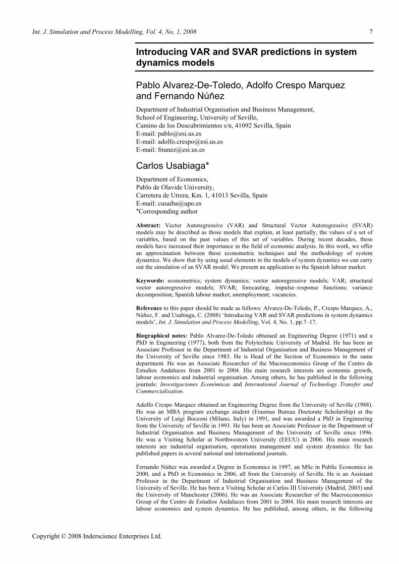
Int. J. Simulation and Process Modelling, Vol. 4, No. 1, 2008 7 Copyright © 2008 Inderscience Enterprises Ltd. Introducing VAR and SVAR predictions in system dynamics models Pablo Alvarez-De-Toledo, Adolfo Crespo Marquez and Fernando Núñez Department of Industrial Organisation and Business Management, School of Engineering, University of Seville, Camino de los Descubrimientos s/n, 41092 Sevilla, Spain E-mail: [email protected] E-mail: [email protected] E-mail: [email protected] Carlos Usabiaga* Department of Economics, Pablo de Olavide University, Carretera de Utrera, Km. 1, 41013 Sevilla, Spain E-mail: [email protected] *Corresponding author Abstract: Vector Autoregressive (VAR) and Structural Vector Autoregressive (SVAR) models may be described as those models that explain, at least partially, the values of a set of variables, based on the past values of this set of variables. During recent decades, these models have increased their importance in the field of economic analysis. In this work, we offer an approximation between these econometric techniques and the methodology of system dynamics. We show that by using usual elements in the models of system dynamics we can carry out the simulation of an SVAR model. We present an application to the Spanish labour market. Keywords: econometrics; system dynamics; vector autoregressive models; VAR; structural vector autoregressive models; SVAR; forecasting, impulse–response functions; variance decomposition; Spanish labour market; unemployment; vacancies. Reference to this paper should be made as follows: Alvarez-De-Toledo, P., Crespo Marquez, A., Núñez, F. and Usabiaga, C. (2008) ‘Introducing VAR and SVAR predictions in system dynamics models’, Int. J. Simulation and Process Modelling, Vol. 4, No. 1, pp.7–17. Biographical notes: Pablo Alvarez-De-Toledo obtained an Engineering Degree (1971) and a PhD in Engineering (1977), both from the Polytechnic University of Madrid. He has been an Associate Professor in the Department of Industrial Organisation and Business Management of the University of Seville since 1983. He is Head of the Section of Economics in the same department. He was an Associate Researcher of the Macroeconomics Group of the Centro de Estudios Andaluces from 2001 to 2004. His main research interests are economic growth, labour economics and industrial organisation. Among others, he has published in the following journals: Investigaciones Económicas and International Journal of Technology Transfer and Commercialisation. Adolfo Crespo Marquez obtained an Engineering Degree from the University of Seville (1988). He was an MBA program exchange student (Erasmus Bureau Doctorate Scholarship) at the University of Luigi Bocconi (Milano, Italy) in 1991, and was awarded a PhD in Engineering from the University of Seville in 1993. He has been an Associate Professor in the Department of Industrial Organisation and Business Management of the University of Seville since 1996. He was a Visiting Scholar at Northwestern University (EEUU) in 2006. His main research interests are industrial organisation, operations management and system dynamics. He has published papers in several national and international journals. Fernando Núñez was awarded a Degree in Economics in 1997, an MSc in Public Economics in 2000, and a PhD in Economics in 2006, all from the University of Seville. He is an Assistant Professor in the Department of Industrial Organisation and Business Management of the University of Seville. He has been a Visiting Scholar at Carlos III University (Madrid, 2003) and the University of Manchester (2006). He was an Associate Researcher of the Macroeconomics Group of the Centro de Estudios Andaluces from 2001 to 2004. His main research interests are labour economics and system dynamics. He has published, among others, in the following
-
Upload
tcpguacimo -
Category
Documents
-
view
1 -
download
0
Transcript of Introducing VAR and SVAR predictions in system dynamics models
Int. J. Simulation and Process Modelling, Vol. 4, No. 1, 2008 7
Copyright © 2008 Inderscience Enterprises Ltd.
Introducing VAR and SVAR predictions in system dynamics models
Pablo Alvarez-De-Toledo, Adolfo Crespo Marquez and Fernando Núñez Department of Industrial Organisation and Business Management, School of Engineering, University of Seville, Camino de los Descubrimientos s/n, 41092 Sevilla, Spain E-mail: [email protected] E-mail: [email protected] E-mail: [email protected]
Carlos Usabiaga* Department of Economics, Pablo de Olavide University, Carretera de Utrera, Km. 1, 41013 Sevilla, Spain E-mail: [email protected] *Corresponding author
Abstract: Vector Autoregressive (VAR) and Structural Vector Autoregressive (SVAR) models may be described as those models that explain, at least partially, the values of a set of variables, based on the past values of this set of variables. During recent decades, these models have increased their importance in the field of economic analysis. In this work, we offer an approximation between these econometric techniques and the methodology of system dynamics. We show that by using usual elements in the models of system dynamics we can carry out the simulation of an SVAR model. We present an application to the Spanish labour market.
Keywords: econometrics; system dynamics; vector autoregressive models; VAR; structural vector autoregressive models; SVAR; forecasting, impulse–response functions; variance decomposition; Spanish labour market; unemployment; vacancies.
Reference to this paper should be made as follows: Alvarez-De-Toledo, P., Crespo Marquez, A., Núñez, F. and Usabiaga, C. (2008) ‘Introducing VAR and SVAR predictions in system dynamics models’, Int. J. Simulation and Process Modelling, Vol. 4, No. 1, pp.7–17.
Biographical notes: Pablo Alvarez-De-Toledo obtained an Engineering Degree (1971) and a PhD in Engineering (1977), both from the Polytechnic University of Madrid. He has been an Associate Professor in the Department of Industrial Organisation and Business Management of the University of Seville since 1983. He is Head of the Section of Economics in the same department. He was an Associate Researcher of the Macroeconomics Group of the Centro de Estudios Andaluces from 2001 to 2004. His main research interests are economic growth, labour economics and industrial organisation. Among others, he has published in the following journals: Investigaciones Económicas and International Journal of Technology Transfer and Commercialisation.
Adolfo Crespo Marquez obtained an Engineering Degree from the University of Seville (1988). He was an MBA program exchange student (Erasmus Bureau Doctorate Scholarship) at the University of Luigi Bocconi (Milano, Italy) in 1991, and was awarded a PhD in Engineering from the University of Seville in 1993. He has been an Associate Professor in the Department of Industrial Organisation and Business Management of the University of Seville since 1996. He was a Visiting Scholar at Northwestern University (EEUU) in 2006. His main research interests are industrial organisation, operations management and system dynamics. He has published papers in several national and international journals.
Fernando Núñez was awarded a Degree in Economics in 1997, an MSc in Public Economics in 2000, and a PhD in Economics in 2006, all from the University of Seville. He is an Assistant Professor in the Department of Industrial Organisation and Business Management of the University of Seville. He has been a Visiting Scholar at Carlos III University (Madrid, 2003) and the University of Manchester (2006). He was an Associate Researcher of the Macroeconomics Group of the Centro de Estudios Andaluces from 2001 to 2004. His main research interests are labour economics and system dynamics. He has published, among others, in the following

8 P. Alvarez-De-Toledo et al.
journals: Revista de Economía Laboral, Revista de Estudios Regionales and Estudios de Economía Aplicada.
Carlos Usabiaga was awarded a Degree in Economics (1988) and a PhD in Economics with distinction (1992), both from the University of Seville. He has been a Visiting Scholar at the London School of Economics (1991 and 1997), Northwestern University (EEUU, 1996), FEDEA (Madrid, 1999), CEMFI (Madrid, 1999), Carlos III University (Madrid, 2001) and European University Institute (Florence, 2004). He is a Full Professor and Head of the Department of Economics, Quantitative Methods and Economic History at Pablo de Olavide University (since 2003 and 2005, respectively). His main research interests are macroeconomics, labour economics and regional economics. He has published papers in many national and international journals. His main book was published by Macmillan.
1 Introduction
Autoregressive (AR), VAR and SVAR models may be described, in general, as those models that explain, at least partially, the values of a variable or set of variables, based on the past values of this variable or set of variables (Box and Jenkins, 1976).1 During recent decades, these models have increased their presence and importance within the field of economics and econometric analysis. It has been found that these kind of simple models, with a small number of variables and parameters, can seriously compete in terms of their forecasting capabilities with the large macroeconomic models, with hundreds of variables and parameters, developed during the 1950s and 1960s.
In this work, we try to offer an approximation between the econometric techniques of the VAR and SVAR models and the methodology of system dynamics. More precisely, we will show that by using usual elements in the models of system dynamics – as the existence of flow and level variables, or the use of optimisation and calibration tools – we can carry out the simulation of an SVAR model – of course, with the previous estimation of its reduced VAR form – to obtain predictions about the behaviour of the endogenous variables of the model. This can be considered as a contribution in the field of the system dynamics, where these types of predictions turn out to be unknown.
When it was necessary to implement some type of prediction on the short-term behaviour (out of the sample period) of one or more variables belonging to a certain system, the system dynamics models have almost exclusively used simple prediction methods derived from time series techniques. Such methods – for instance, exponential smoothing or trend extrapolation methods (Roberts, 1978; Richardson and Pugh, 1981; Sterman, 2000)2 – present two essential features: on the one hand, they have a univariate character, since they only use lagged values of the same variable to formulate the predictions; on the other hand, they are deterministic methods, not parametric, since when a prediction is formulated, authors do not pay attention to the stochastic nature of the population from which it is supposed that the available observations have been extracted.
Nevertheless, the aforementioned naive methods of time series have been opening a way in recent decades to more
complex prediction techniques, which are characterised essentially for their multivariate structure, allowing for the existence of relations (contemporary and with time delays) among a group of variables, and also for considering the stochastic nature of the variables. This is the case of the VAR and SVAR models, whose methodology has not been used in system dynamics to formulate predictions yet, probably owing to the difficulty in transferring the foundations of the above-mentioned methodology to the language of system dynamics.
In this work, we will use the foundations of the VAR and SVAR models to develop a simulation language tool – macro – that can be used with system dynamics models to carry out two types of predictions regarding the behaviour of certain variables, which are interrelated. The type of prediction will depend on the model that we use: SVAR or its reduced form (VAR model). The VAR models are commonly used for forecasting (in the short term) systems of interrelated time series out of the sample period. These models, unlike the SVAR models, are characterised because they only handle the information contained in the sample, and do not impose restrictions based on Economic Theory.3 Therefore, they are especially advisable when we have scanty information of theoretical nature or this information lacks a sufficiently widespread acceptance.
The VAR models can be seen as a reduced form of SVAR models, which use the available theoretical information (extra-sample information) to build the contemporary relations among the endogenous variables of the model. The more we trust the theoretical information that we refer to, the more advisable this practice would be.
It has been demonstrated that SVAR models can be formulated as the result of non-recursive (or structural) orthogonalisation of the innovation terms of a (reduced form) VAR model; this alternative to the recursive Cholesky orthogonalisation requires the researcher to impose enough theoretical restrictions to identify the orthogonal (structural) components of the error terms. In this form, an SVAR model allows one to simulate the dynamic impact of orthogonal structural shocks on the system of variables, and therefore, the type of prediction that they offer – where the system variables are subjected to impulses – differs in nature from those predictions offered by VAR
Introducing VAR and SVAR predictions in system dynamics models 9
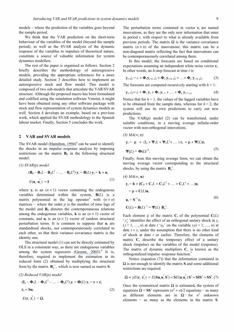
models – where the prediction of the variables goes beyond the sample period.
We think that the VAR prediction on the short-term behaviour of the variables of the model (beyond the sample period), as well as the SVAR analysis of the dynamic response of the variables to impulses of theoretical nature, constitute a source of valuable information for system dynamics modellers.
The rest of the paper is organised as follows. Section 2 briefly describes the methodology of autoregressive models, providing the appropriate references for a more detailed study. Section 3 describes how to implement an autoregressive stock and flow model. This model is composed of two sub-models that articulate the VAR/SVAR structure. Although the proposed macro has been formulated and codified using the simulation software Vensim, it might have been obtained using any other software package with stock and flow representation of system dynamics models as well. Section 4 develops an example, based on a previous work, which applied the SVAR methodology to the Spanish labour market. Finally, Section 5 concludes the work.
2 VAR and SVAR models
The SVAR model (Hamilton, 1994)4 can be used to identify the shocks in an impulse–response analysis by imposing restrictions on the matrix B0 in the following structural model:
(1) SVAR(p) model
(B0 – B1L – B2L2 – … – BpLp) yt = B(L) yt = k + ut
( ) =t tE ′u u I (1)
where yt is an (n × 1) vector containing the endogenous variables determined within the system, B(L) is a matrix polynomial in the lag operator5 with (n × n) matrices − where the order p is the number of time lags of the model and B0 denotes the contemporaneous relations among the endogenous variables, k is an (n × 1) vector of constants, and ut is an (n × 1) vector of random structural perturbation terms. It is common to suppose that ut are standardised shocks, not contemporaneously correlated to each other, so that their variance–covariance matrix is the identity one.
The structural model (1) can not be directly estimated by OLS in a consistent way, as there are endogenous variables among the system regressors (Greene, 2003).6 It is, therefore, required to implement the estimation in its reduced form (2) obtained by multiplying the structural form by the matrix 1
0 ,−B which is now named as matrix S.
(2) Reduced VAR(p) model
(In – Φ1L – Φ2L2 – … – ΦpLp) yt = Φ(L) yt = c + εt
εt = Sut (2)
( ) =t tE ′ .ε ε Ω
The perturbation terms contained in vector εt are named innovations, as they are the only new information that enter in period t, with respect to what is already available from previous periods. The matrix Ω is the variance–covariance matrix (n × n) of the innovations; this matrix can be a non-diagonal matrix reflecting the fact that innovations can be contemporaneously correlated among them.
In this model, the forecasts are based on conditional expectations assuming an independent white noise vector εt. In other words, an h-step forecast at time t is:
yt+h|t = c + Φ1yt+h–1|t + Φ2 yt+h–2|t + …+ Φp yt+h–p|t. (3)
The forecasts are computed recursively starting with h = 1:
yt+1|T= c + Φ1 yt + Φ2 yt–1 + … + Φp yt+1–p. (4) Notice that for h = 1, the values of the lagged variables have to be obtained from the sample data, whereas for h > 2, the system will use its own predictions to carry out new predictions.
The VAR(p) model (2) can be transformed, under suitable conditions, in a moving average infinite-order vector with non-orthogonal innovations.
(3) MA(∞, ε)
yt = µ + (In + Ψ1L + Ψ2L2+ … ) εt = µ + Ψ(L)εt
Ψ(L) = Φ(L)–1. (5)
Finally, from this moving average form, we can obtain the moving average vector corresponding to the structural shocks, by using the matrix 1
0 .−B
(4) MA(∞, u)
yt = h + (C0 + C1L + C2L2 + … + CsLs + …)ut
= µ + C(L)ut
ut = S−1 εt (6)
C(L) = B(L)–1 = Ψ(L) 10 .−B
Each element ij of the matrix Cs of the polynomial C(L) ‘ s
ijc ’identifies the effect of an orthogonal unitary shock in yj ( j = 1, …, n) at date t ‘ujt’ on the variable yi(i = 1, …, n) at date t + s, under the assumption that there is no other kind of shock at date t or earlier. Therefore, the elements of matrix Cs describe the temporary effect of a unitary shock (impulse) on the variables of the model (response). The matrix of dynamic multipliers Cs is known as the orthogonalised impulse–response function.7
Notice (equation (7)) that the information contained in Ω is not enough to identify the matrix S and some additional restrictions are required.
y ( ) = ( ) ( ) .t t t t t tE E E′ ′′ ′ ′ ′ ′= = =Su u S S u u S SIS SSΩ = ε ε (7)
Once the symmetrical matrix Ω is estimated, the system of equations Ω = SS´ represents (n2 + n)/2 equations − as many as different elements are in Ω − for n2 unknown elements − as many as the elements in the matrix S.
10 P. Alvarez-De-Toledo et al.
Therefore, (n2 − n)/2 are the additional restrictions required to solve the system. In the SVAR models, these additional restrictions can be obtained from the implications of theoretical models on the expected behaviour of the variables yt.
3 The design of a structural autoregressive stock and flow model in Vensim
We will now show how it is possible to implement a stock and flow VAR/SVAR model using Vensim.8 We will explain how we have implemented this model by constructing two basic stock-flow sub-models (sub-model 1 and sub-model 2), each of which corresponds to different phases of the analytical process, as shown in detail later. We want to remark here that it is not the purpose of this paper to design a system dynamics model, but to provide a sort of ‘macro’ that will facilitate the system dynamics modellers to incorporate elements of the VAR and SVAR methodology.
The core of both sub-models is the forecast of the variables in every period from their values in the previous periods, according to the reduced autoregressive form of equation (2). The main difference between both sub-models is that sub-model 1 uses the real data of the variables in the previous periods, whereas sub-model 2 uses the forecasts for the previous periods provided by the own sub-model. For this reason, we can point out that the forecast horizon is of single period in the first sub-model, and multi-period in the second one.
Sub-model 1 is used to estimate the parameters of the model in the reduced autoregressive form (2) from a series of real values of the variables. This sub-model analyses the fit between the forecasts of the estimated model (2) and the series of real values of the variables, computing the differences between them (residuals or estimated values of innovations εt) and their variance–covariance matrix.
Once we obtain the values of the estimated parameters, sub-model 2 can be used for two purposes: obtaining a VAR prediction of the endogenous variables several time periods in advance, and simulating the response of the variables to different impulses in structural shocks ut – impulse–response functions. For this second task, sub-model 2 is used to calculate the matrix B0 with the additional restrictions that the theoretical model imposes on the dynamics of the variables. In the following step, we can obtain the structural autoregressive form from the reduced autoregressive form and simulate the structural impulse–response functions. These functions are also related to the moving average forms of the model. To obtain all these results, three versions of sub-model 2 are used, differing only in the magnitude of the innovations.
In the next two sub-sections, we present the analytical process that both sub-models follow in detail.
3.1 Detailed explanation of sub-model 1
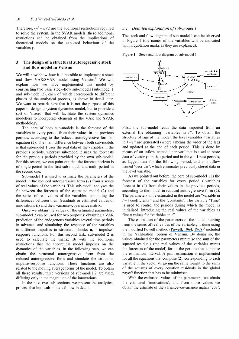
The stock and flow diagram of sub-model 1 can be observed in Figure 1 (the names of the variables will be indicated within quotation marks as they are explained).
Figure 1 Stock and flow diagram of sub-model 1
First, the sub-model reads the data imported from an external file obtaining “variables in t ”. To obtain the structure of lags of the model, the level variables “variables in t − i ” are generated (where i means the order of the lag) and updated at the end of each period. This is done by means of an inflow named ‘incr var’ that is used to store data of vector yt, in that period and in the p − 1 past periods, as lagged data for the following period, and an outflow named ‘decr var’, which eliminates previously stored data in the level variable.
As we pointed out before, the core of sub-model 1 is the forecast of the variables for every period (“variables forecast in t ”) from their values in the previous periods, according to the model in reduced autoregressive form (2). The parameters to be estimated in the model are “variable in t − i coefficients ” and the ‘constants’. The variable ‘Time’ is used to control the periods during which the model is initialised, introducing the real values of the variables as first p values for “variables in t ”.
The estimation of the parameters of the model, starting from the series of real values of the variables, is done using the modified Powell method (Powell, 1964, 1968)9 included in the ‘calibration’ option of Vensim. By doing so, the values obtained for the parameters minimise the sum of the squared residuals (the real values of the variables minus the forecasts of the model) for all the periods that compose the estimation interval. A joint estimation is implemented for all the equations that compose (2), corresponding to each variable in the vector yt, giving the same weight to the sums of the squares of every equation residuals in the global payoff function that has to be minimised.
With the estimated values of the parameters, we obtain the estimated ‘innovations’, and from those values we obtain the estimate of the variance–covariance matrix ‘cov’.
Introducing VAR and SVAR predictions in system dynamics models 11
The flow variable ‘inc’ increases, in every period, the accumulated level ‘previous cov’ of the sum of the residuals products for all the previous periods. Finally, the variable ‘FINAL TIME’ provides the number of periods that are necessary to take into account in this process.
3.2 Detailed explanation of sub-model 2
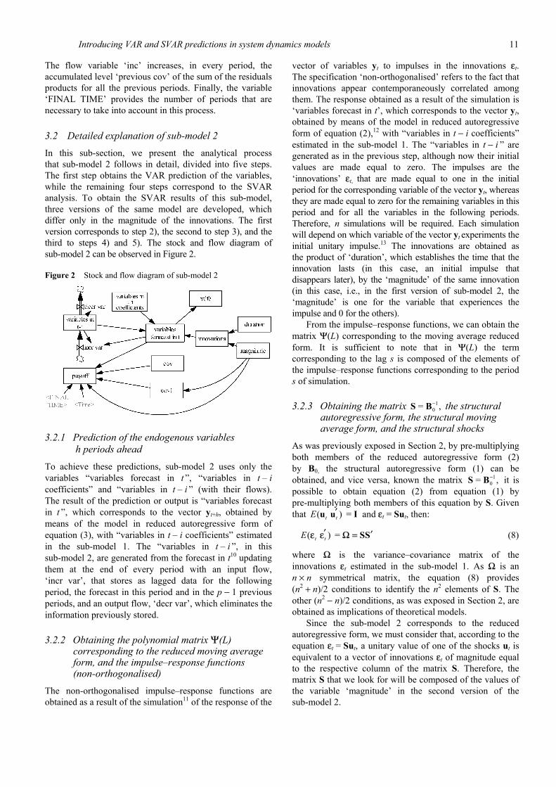
In this sub-section, we present the analytical process that sub-model 2 follows in detail, divided into five steps. The first step obtains the VAR prediction of the variables, while the remaining four steps correspond to the SVAR analysis. To obtain the SVAR results of this sub-model, three versions of the same model are developed, which differ only in the magnitude of the innovations. The first version corresponds to step 2), the second to step 3), and the third to steps 4) and 5). The stock and flow diagram of sub-model 2 can be observed in Figure 2.
Figure 2 Stock and flow diagram of sub-model 2
3.2.1 Prediction of the endogenous variables h periods ahead
To achieve these predictions, sub-model 2 uses only the variables “variables forecast in t ”, “variables in t – i coefficients” and “variables in t – i ” (with their flows). The result of the prediction or output is “variables forecast in t ”, which corresponds to the vector yt+h, obtained by means of the model in reduced autoregressive form of equation (3), with “variables in t – i coefficients” estimated in the sub-model 1. The “variables in t – i ”, in this sub-model 2, are generated from the forecast in t10 updating them at the end of every period with an input flow, ‘incr var’, that stores as lagged data for the following period, the forecast in this period and in the p − 1 previous periods, and an output flow, ‘decr var’, which eliminates the information previously stored.
3.2.2 Obtaining the polynomial matrix Ψ(L) corresponding to the reduced moving average form, and the impulse–response functions (non-orthogonalised)
The non-orthogonalised impulse–response functions are obtained as a result of the simulation11 of the response of the
vector of variables yt to impulses in the innovations εt. The specification ‘non-orthogonalised’ refers to the fact that innovations appear contemporaneously correlated among them. The response obtained as a result of the simulation is ‘variables forecast in t’, which corresponds to the vector yt, obtained by means of the model in reduced autoregressive form of equation (2),12 with “variables in t − i coefficients” estimated in the sub-model 1. The “variables in t − i ” are generated as in the previous step, although now their initial values are made equal to zero. The impulses are the ‘innovations’ εt, that are made equal to one in the initial period for the corresponding variable of the vector yt, whereas they are made equal to zero for the remaining variables in this period and for all the variables in the following periods. Therefore, n simulations will be required. Each simulation will depend on which variable of the vector yt experiments the initial unitary impulse.13 The innovations are obtained as the product of ‘duration’, which establishes the time that the innovation lasts (in this case, an initial impulse that disappears later), by the ‘magnitude’ of the same innovation (in this case, i.e., in the first version of sub-model 2, the ‘magnitude’ is one for the variable that experiences the impulse and 0 for the others).
From the impulse–response functions, we can obtain the matrix Ψ(L) corresponding to the moving average reduced form. It is sufficient to note that in Ψ(L) the term corresponding to the lag s is composed of the elements of the impulse–response functions corresponding to the period s of simulation.
3.2.3 Obtaining the matrix 10= ,−S B the structural
autoregressive form, the structural moving average form, and the structural shocks
As was previously exposed in Section 2, by pre-multiplying both members of the reduced autoregressive form (2) by B0, the structural autoregressive form (1) can be obtained, and vice versa, known the matrix 1
0= ,−S B it is possible to obtain equation (2) from equation (1) by pre-multiplying both members of this equation by S. Given that ( ) =t tE ′u u I and εt = Sut, then:
( ) =t tE ′ ′SSε ε Ω = (8)
where Ω is the variance–covariance matrix of the innovations εt estimated in the sub-model 1. As Ω is an n × n symmetrical matrix, the equation (8) provides (n2 + n)/2 conditions to identify the n2 elements of S. The other (n2 − n)/2 conditions, as was exposed in Section 2, are obtained as implications of theoretical models.
Since the sub-model 2 corresponds to the reduced autoregressive form, we must consider that, according to the equation εt = Sut, a unitary value of one of the shocks ut is equivalent to a vector of innovations εt of magnitude equal to the respective column of the matrix S. Therefore, the matrix S that we look for will be composed of the values of the variable ‘magnitude’ in the second version of the sub-model 2.

12 P. Alvarez-De-Toledo et al.
The numerical optimisation is guided by the fulfilment of the aforementioned conditions, by means of the maximisation of a vector of n2 variables ‘payoff’, giving the same weight to all these variables. The first (n2 − n)/2 variables capture the theoretical restrictions required for the identification of the SVAR model, while the remaining (n2 + n)/2 guarantees the fulfilment of equation (8). Regarding the theoretical restrictions, sometimes they directly influence the matrix 1
0= ,−S B while in other cases, as it happens in our application, they affect the dynamic forecasts of the model acting indirectly on S. The additional (n2 + n)/2 restrictions are the square of the differences among all non-identical elements of the symmetrical matrices SS′ and Ω, with negative sign. In the second version of the sub-model 2, we impose initial unitary values to all the elements of ‘magnitude’, and therefore to all the elements of S. After that, the process of optimisation continues until the values of the above-mentioned elements that approximate the payoff sufficiently to its maximum possible value are found. In this maximum value, the last (n2 + n)/2 variables of the payoff function will have a value equal to zero and the theoretical restrictions will be fulfilled. The variables ‘cov’ and ‘cov1’ (with the corresponding subscripts) are, respectively, the elements of the matrix Ω estimated in the sub-model 1, and the elements of the product SS′, obtained from the values of ‘magnitude’ that form the matrix S. The variables ‘Time’ and ‘FINAL TIME’ are used to control that the payoff is calculated in the period corresponding to the theoretical restrictions used.
Once the matrix 10= −S B has been obtained,
pre-multiplying both members of the reduced autoregressive form (2) by B0, the structural autoregressive form (1) and the structural shocks ut = B0 εt are obtained. The structural moving average form (6) can also be obtained from the moving average reduced form (5) (obtained in step 1), by multiplying Ψ(L) by S, since, as εt = Sut, we get:
yt = Ψ(L) εt + … = Ψ(L) SS–1 εt + … = C(L) ut + … (9)
where C(L) = Ψ(L)S is the polynomial matrix corresponding to the structural moving average form.
3.2.4 Obtaining the orthogonalised impulse–response functions
In the third version of sub-model 2, the elements of ‘magnitude’ are made equal to the values obtained for S in the previous step. Each of the parallel simulations conducted with the reduced autoregressive form corresponds to unitary values in the initial period of each of the structural shocks. Therefore, the values obtained in the simulations of the variables in “variables forecast in t ” represent the orthogonalised impulse–response functions for these variables. The specification ‘orthogonalised’ refers to the fact that the structural shocks are not contemporaneously correlated among each other.
3.2.5 Variance decomposition of the forecasting error
From the values, in each period, of the forecasts of the variables in the orthogonalised impulse–response functions of the previous step, we can obtain the decomposition of the variance of the forecasting error ‘vdfe’ in the same period. This forecasting error originates from the responses to each one of the n structural shocks. So, for each variable, the percentage that supposes the square of its value in each simulation is calculated in relation to the sum of all the squares.
4 An application to the Spanish labour market
We now present an application of the model explained in the previous section, implementing in Vensim an SVAR model referred to the Spanish labour market (Blanchard and Quah, 1989; Bean, 1992; Galí, 1992),14 developed by Dolado and Gómez (1997) and Usabiaga et al. (2001),15 following Blanchard and Diamond (1989).
The SVAR model of Dolado and Gómez (1997) focuses on the quarterly series of three variables: unemployment (U), vacancies (V), and labour force (L). As we will show, in this model the vector yt is obtained from a few previous transformations, and is composed of the variables v1 = ∆(v − u), v2 = ∆u and v3 = ∆l; where v, u and l are the logarithms of V, U and L, and where ∆ indicates the first difference of the corresponding variable. These three transformed variables correspond, respectively, to the growth rates of the vacancies/unemployment ratio, unemployment and labour force.
Relating each of these three transformed variables with the lagged values (up to four quarters) of all of them, the reduced autoregressive form (2) is derived, including also a vector of quarterly dummy variables dt with its coefficients matrix D, to control the seasonal effects:
Φ(L) yt = c + D dt + εt (10)
As was mentioned in Section 2, in this reduced autoregressive form, contemporaneous relations do not appear among the variables, i.e., each variable is not related to the values of the others in the same period. These contemporaneous relations do appear in the structural autoregressive form (1). The matrix B0, within the polynomial in the lag operator B(L), reflects the contemporaneous relations among the variables. As exposed in Section 2, the information contained in the estimated matrix Ω is not sufficient to identify the elements of B0, and therefore, it is necessary to add restrictions. These restrictions can be obtained from the implications that theoretical models may have on the expected behaviour of the variables yt.
Dolado and Gómez (1997) use a theoretical model, following a flow approach (Blanchard and Diamond, 1992; Pissarides, 2000)16 to labour markets, made up of four

Introducing VAR and SVAR predictions in system dynamics models 13
blocks: the flows of job creation and job destruction, the hiring process through a matching function between vacancies and unemployment, the wage determination as a function of the excess of demand in the labour market, and the labour supply or labour force as a function of wages and unemployment. All these elements are used to obtain a relation among the transformed variables that compose the vector yt in the structural autoregressive form (1). At the same time, the structural shocks ut, are identified using three types of disturbances in the economy:
• aggregate activity shocks, owing to disturbances in the different components of aggregate demand
• reallocation shocks, owing to disturbances affecting the efficiency of the matching process between vacancies and unemployment (skill mismatch, geographical mismatch, etc.)
• labour force shocks, owing to disturbances that affect directly this variable (women’s participation in the labour market, etc.).
The additional restrictions for the identification of B0, obtained as implications of this theoretical model, are that a labour force shock does not have permanent effects on unemployment and vacancies, and that a reallocation shock does not have permanent effects on the vacancies/unemployment ratio.
To develop this application with Vensim, we are going to follow the steps described in the previous section with both sub-models. Since these steps correspond faithfully to those followed in the process of econometric estimation of an SVAR model, the numerical results obtained are practically identical to those of Dolado and Gómez (1997).17 In this application, the sub-models 1 and 2 are denoted as ‘labour 1’ and ‘labour 2’, respectively.
4.1 Sub-model labour 1
The stock and flow diagram corresponding to the sub-model labour 1 is presented in Figure 3.
Figure 3 Stock and flow diagram of labour 1
First, the model reads the ‘data’ imported from an external file: quarterly series of values for V, U and L, besides the quarterly dummy variables. The sample period goes from 1977 : 01 to 1994 : 04, as in Dolado and Gómez (1997).
Second, several data initial transformations are made, obtaining “variables in t ” and the ‘dummies’. The variables obtained are v1, v2 and v3, composing the vector yt. To calculate these differences, the level variables ‘data in t − 1’ need to be calculated first, and are updated at the end of every period with an inflow ‘incr dat’ that stores the data of this period as lagged information for the following period, and an outflow ‘decr dat’ that eliminates the data stored previously. Moreover, the four seasonal dummies (d1, d2, d3, d4) are reduced to three (t1, t2, t3), to avoid the problem of perfect collinearity among them, defining:
t1 = d1 – d4
t2 = d2 – d4 (11)
t3 = d3 – d4.
As we pointed out previously, the core of labour 1 is the forecast of the variables for every period “variables forecast in t ” from their values in the previous periods. The parameters to be estimated in the model are “variable coefficients in t − i ”, ‘dummies coefficients’ and the ‘constants’. Using the ‘calibration' option of Vensim, with sub-model labour 1, the following values are obtained for the parameters:
0.02270.01540.0023
0.1266 1.3112 7.57040.0174 0.5078 0.61070.0026 0.0215 0.1264
0.2134 0.3097 0.90930.0073 0.1930 2.1762
0.0002 0.0439 0.0313
−=
−+ − − +
− −
−+ − − +
− −
+
v1 't'v2 't'v3 't'
v1 't 1'v2 't 1'v3 't 1'
v1 't 2'v2 't 2'v3 't 2'
−−−
−−−
0.2090 0.1916 6.15991.0103 0.1398 1.1385
0.0007 0.0039 0.1545
0.0646 0.9359 7.83550.0368 0.1115 2.48650.0009 0.0313 0.0049
0.0562 0.3256 0.21870.0095 0.0570 0.02750
− −− − +
+ − +
− −+ −
−
v1 't 3'v2 't 3'v3 't 3'
v1 't 4'v2 't 4'v3 't 4'
−−−
−−−
..0008 0.0005 0.0048−
t1t2t3
With the estimated values of the parameters, we obtain the estimated ‘innovations’ and the estimate of the variance–covariance matrix ‘cov’:

14 P. Alvarez-De-Toledo et al.
0.020200 0.000163 0.0000910.000163 0.000386 0.000017 .
0.000091 0.000017 0.000010
v1 v2 v3v1v2v3
−−
4.2 Sub-model labour 2
The stock and flow diagram corresponding to the sub-model labour 2 is presented in Figure 4.
Figure 4 Stock and flow diagram of labour 2
4.2.1 Prediction of the endogenous variables h periods ahead
In this step, “variables forecast in t ” shows the predicted values for the variables contained in yt (v1, v2 and v3) beyond the last sample data (which is 1994 : 4). The model recovers the levels v − u, u and l accumulating the forecast in the variable ‘accumulated forecast’. The level ‘previous accumulated forecast’ is updated at the end of every period with the inflow ‘inc previous accumulated forecast’, which is equal to the forecast of the variables obtained in this period, and ‘accumulated forecast’ is obtained by adding this forecast to the one accumulated previously (notice that the updating of the level variables at the end of every period is not registered in the output of the model until the following period). ‘Accumulated forecast v’ is then obtained adding the levels v − u and u.
As an example, we represent in Figure 5 the predicted values for the variables u, v and l, between 1995 : 01 and 1997 : 02.
Figure 5 Predicted series. 1995 : 01–1997 : 02
We would like to highlight that this type of prediction may have a wide application for many different types of system dynamics models: product demand behaviour, number of births, etc.
4.2.2 Obtaining the polynomial matrix Ψ(L) corresponding to the reduced moving average form, and the impulse–response functions (non-orthogonalised)
In our application to the labour market, the terms of Ψ(L) are 3 × 3 matrices and their elements correspond to the response of each one of the three variables (v1, v2, v3) to each one of the three simulated unitary impulses.18
4.2.3 Obtaining the matrix 10= ,−S B the structural
autoregressive form, the structural moving average form, and the structural shocks
As in our example, Ω is a 3 × 3 symmetrical matrix, the equation (8) provides six conditions to identify the nine elements of S. The other three conditions are obtained as implications of the theoretical model. These conditions are that a labour force shock does not have permanent effects on unemployment and vacancies, and that a reallocation shock does not have permanent effects on the vacancies/unemployment ratio.
The numerical optimisation is guided by the fulfilment of the aforementioned conditions, by means of the maximisation of a vector of nine variables ‘payoff ’, giving the same weight to all these variables. The first three ([po1], [po2], [po3]) are the square of the forecast in the final period (long term) of u and v, responding to an unitary labour force shock, and the square of the forecast in the final period of v − u responding to an unitary reallocation shock, all of them with negative sign. The other six ([po4], [po5], [po6], [po7], [po8], [po9]) are the square of the differences among all six non-identical elements of the symmetrical matrices SS′ and Ω, also with negative sign. That value of S is reached when Ω = SS′, and the forecast of u and v in the final period responding to a unitary labour force shock, and the forecast of v − u in the final period responding to a unitary reallocation shock are all of them equal to zero. Remember that the matrix S that we look for will be composed of the values that the variable ‘magnitude’ takes in our model (of each innovation in each of the three simulations). The result obtained from the simulation is as follows:
0.1161 0.0745 -0.03430.0054 0.0127 0.014
0.0018 0.0006 0.0025= −
−S
Notice that the properties of the theoretical model refer to the values of u, v and v − u in the long term, acting therefore on the accumulated forecasts.

Introducing VAR and SVAR predictions in system dynamics models 15
4.2.4 Obtaining the orthogonalised impulse–response functions
In the third version of labour 2, the elements of ‘magnitude’ are made equal to the values obtained for S in the previous step. Therefore, the values obtained in the simulations of the variables u and l in ‘accumulated forecast’, and of v in ‘accumulated forecast v’, represent the orthogonalised impulse–response functions for these variables, recovered from their first differences. The specification ‘orthogonalised’ refers to the fact that the structural shocks are not contemporaneously correlated among each other.
As an example, we represent in Figure 6 the impulse–response functions obtained for u. A positive shock of aggregate activity (j1) permanently reduces unemployment, whereas a positive reallocation shock (j2) causes a permanent increase of the same variable. Finally, a positive labour force shock (j3) increases unemployment slightly in the short term; however, in the long term, as job creation and job destruction adjust to the decrease of the real wages associated with the increase of unemployment, the effects on unemployment will tend to disappear.
Figure 6 Orthogonalised impulse-response functions. Unemployment
In general, a simulation of this type can be of interest to analyse the behaviour of a certain system dynamics model (demographic, managerial, ecological, etc.) when disturbances appear. For instance, our model is used to simulate the response of the vacancies and unemployment variables to the three perturbations that we have considered. These responses can be used as inputs of the entry flow to the employment level variable. Notice that, for instance, the employment level could be considered as a variable of a more generic model of the economy.
4.2.5 Variance decomposition of the forecasting error
From the values, in each period, of u and l in ‘accumulated forecast’ and v in ‘accumulated forecast v’ in the orthogonalised impulse–response functions of the previous step, we can obtain the variance decomposition of the forecasting error ‘vdfe’ in the same period for u, l and v. This forecasting error originates from the responses to each one of the three structural shocks.
As an illustration, in Figure 7, we represent the variance decomposition of the forecasting error for u. In the very short term, the structural shocks with more weight in unemployment variability are labour force (j3) and reallocation (j2). However, in the medium and long term, reallocation (j2) and aggregate activity (j1) shocks completely explain the unemployment variability.19
Figure 7 Variance decomposition of the forecasting error. Unemployment
5 Concluding remarks
Our main goal has been the creation of a tool or ‘macro’ to be used with Vensim simulation environment, which when applied to a given system dynamics model, provides autoregressive endogenous structure and short-term forecasting capabilities. The main effort has been done by searching for the correspondence, in stock-flow modelling, of the main concepts and procedures that characterise the VAR and SVAR models.
To develop this stock-flow version of the VAR/SVAR model, we have built two sub-models using the Vensim simulation environment. Each of these sub-models corresponds to different phases of the process of the VAR/SVAR analysis. The lagged variables, essential in the autoregressive analysis, are now treated as level variables. The calculation procedures have been similar to those of the original econometric VAR/SVAR analysis, although the analytical resolution of some of the steps of the problem has been done through simulation within the stock-flow sub-models.
The core of the stock-flow sub-models built is the reduced autoregressive form (VAR model) of the SVAR system. The second sub-model uses the coefficients that were estimated in the first sub-model with two different purposes: providing VAR prediction on the short-term behaviour of the endogenous variables of the model beyond the sample period; and analysing the response of the variables to structural shocks, which have been obtained transforming the innovations of the VAR system into non-orthogonalised perturbations by means of the corresponding matrix, which has been also estimated with the second sub-model. In our opinion, all this analysis implies a relevant contribution in the field of system dynamics.

16 P. Alvarez-De-Toledo et al.
As an illustration, we present an application to the study of the Spanish labour market. The results obtained (estimates of the parameters, predicted variables, impulse–response functions, decomposition of the variance of the forecasting error) with the stock-flow sub-models reproduce faithfully those of the original application of the VAR/SVAR analysis.
References Bean, C. (1992) ‘Identifying the causes of British unemployment’,
Center for Economic Performance, Working Paper No. 276, London School of Economics.
Blanchard, O.J. and Diamond, P. (1989) ‘The Beveridge curve’, Brookings Papers on Economic Activity, Vol. 1, pp.1–60.
Blanchard, O.J. and Diamond, P. (1992) ‘The flow approach to labour markets’, American Economic Review, Vol. 82, No. 2, pp.354–359.
Blanchard, O.J. and Quah, D.T. (1989) ‘The dynamic effects of aggregate demand and supply disturbances’, American Economic Review, Vol. 79, No. 4, pp.655–673.
Box, G.E.P. and Jenkins, G.M. (1976) Time Series Analysis: Forecasting and Control, Holden Day, San Francisco.
Dolado, J.J. and Gómez, R. (1997) ‘La relación entre desempleo y vacantes en españa: perturbaciones agregadas y de reasignación’, Investigaciones Económicas, Vol. 21, No. 3, pp.441–472.
Galí, J. (1992) ‘How well does the IS-LM model fit Postwar US data?’, Quarterly Journal of Economics, Vol. 107, No. 2, pp.709–738.
Greene, W.H. (2003) Econometric Analysis, 5th ed., Prentice Hall, New York.
Hamilton, J.D. (1994) Time Series Analysis, Princeton University Press, Princeton.
Pissarides, C.A. (2000) Equilibrium Unemployment Theory, MIT Press, Cambridge, Mass.
Powell, M.J.D. (1964) ‘An efficient method for finding the minimum of a function of several variables without calculating derivatives’, Computer Journal, Vol. 7, No. 2, pp.155–162.
Powell, M.J.D. (1968) ‘On the calculation of orthogonal vectors’, Computer Journal, Vol. 11, No. 2, pp.302–304.
Richardson, G.P. and Pugh, A.L. (1981) Introduction to System Dynamics Modelling with Dynamo, MIT Press, Cambridge, Mass.
Roberts, E.B. (1978) Managerial Applications of System Dynamics, Productivity Press, Cambridge, Mass.
Sterman, J. (2000) Business Dynamics: Systems Thinking and Modelling for a Complex World, McGraw-Hill, New York.
Usabiaga, C. (Dir.) Álvarez-de-Toledo, P., Crespo, A. and Núñez, F. (2001) Comparación entre las Técnicas de Análisis Shift-Share y de Economías Virtuales, Vector Autorregresivo y Dinámica de Sistemas: Aplicaciones al Mercado de Trabajo Andaluz, Research Project financed by the Andalusian Government, Andalusian Statistics Office.
Notes 1These models are included in the groups of ARIMA and VARIMA models, which follow the Box–Jenkins methodology – see Box and Jenkins (1976).
2Some illustrations of the use of these techniques in system dynamics can be found in Roberts (1978), Richardson and Pugh (1981) and Sterman (2000).
3It is important to note that these models are not completely independent of the theory, because the selection of the variables included in the model must be inspired in a theoretical intuition.
4An explanation of the methodology of autoregressive models (AR, VAR and SVAR) can be found in Hamilton (1994).
5The lag operator L is defined as follows: Lxt ≡ xt–1; L2xt ≡ xt–2; … Lpxt ≡ xt–p.
6This problem in the OLS estimation of the models in its structural form is discussed in Greene (2003).
7Another basic element in the SVAR analysis, besides the impulse–response function, is the variance decomposition of the forecasting error, from which it is possible to study the relative weight of each shock in the variability of the endogenous variables of the model.
8We have used Vensim 4.0, which is a Trade Mark of Ventana System Inc.
9Among the numerical optimisation techniques, the direct-search method that does not evaluate the gradient is the most suitable for the analysis of the dynamics of complex non-linear control systems. The Powell method (Powell, 1964) is well known in order to have an ultimate fast convergence among direct-search methods. The basic idea behind the Powell method is to break the N-dimensional minimisation down into N separate one-dimensional (1D) minimisation problems. Then, for each 1D problem, a binary search is implemented to find the local minimum within a given range. Furthermore, in subsequent iterations, an estimate is obtained for the best directions to use for the 1D searches. Some problems, however, are not always assured of optimal solutions because the direction vectors are not always linearly independent. To overcome this difficulty, the method was revised (Powell, 1968) by introducing new criteria for the formation of linearly independent direction vectors. This revised method, which is the one used in this paper, is denoted as ‘the modified Powell method’.
10Initially, their values are made equal to the last p sample periods. 11See Hamilton (1994). 12In contrast with equation (3), it can be observed that equation (2)
incorporates a vector of contemporaneous innovations εt. 13If it is necessary to compute several simulations of the same
model, the use of subscripts allows us to carry out all the simulations at the same time. Vensim allows the use of those subscripts.
14Pioneering works in the application of the SVAR analysis to the labour market are Blanchard and Quah (1989), Bean (1992) and Galí (1992). In another line, we have seen that models involving rational expectations can be represented as an SVAR model. The resultant structural shocks represent the ‘news’ in the variable that cannot be explained by other variables of the system and, therefore, measure the autonomous contribution to the

Introducing VAR and SVAR predictions in system dynamics models 17
respective variables. It is logical to focus on the dynamic effects of such shocks when assessing the impact of political instruments on the target variables. In comparison with other fields, the relation between the SVAR models and the formation of expectations is not strong in the macroeconomic models of the labour market, may be due to the features of the variables involved.
15Other contribution in this line, for the Andalusian labour market, is Usabiaga et al. (2001).
16A detailed analysis of the labour market, following the flow approach, can be found in Blanchard and Diamond (1992) and Pissarides (2000).
17We have replicated the analysis developed in Dolado and Gómez (1997) using the econometric software Eviews 3.1.
18The numerical results obtained at this step are not relevant since impulse–response functions are non-orthogonalised.
19An important feature of the SVAR methodology is that the results obtained from the analysis of the impulse–response functions and the variance decomposition of the forecasting error are related to the identification restrictions adopted.