The Discounted economic stock of money with VAR forecasting
26
William A. Barnett, Unja Chae, and John W. Keating The Discounted economic stock of money with VAR forecasting Received: /Accepted: Abstract We measure the economic capital stock of money implied by the Divisia monetary aggregate service flow, in a manner consistent with asset pricing theory. Based on Barnett’s [4] definition of the economic stock of money, we estimate the expected discounted flow of expenditure on the services of monetary assets, where expenditure on monetary services is evaluated at the user costs of the monetary components. We use forecasts based on martingale expectations, asymmetric vector autoregressive expectations, and the Bayesian vector autoregressive expectations. We find the resulting capital-stock index to be surprisingly robust to the modeling of expectations. Keywords Monetary aggregation, Divisia money aggregate, economic stock of money, user cost of money, currency equivalent index, Bayesian vector autoregression, asymmetric vector autoregression. JEL Classifications E41 G12 C43 C22 E5. Corresponding author: William A. Barnett Department of Economics, University of Kansas, Lawrence, KS 66045-7585, USA. Phone: 785-864-2844. Fax: 785-864-5760. E-mail: [email protected]. Web: http://alum.mit.edu/www/barnett. Unja Chae Intel Corporation, 2200 Mission College Blvd., Santa Clara, CA 95052, USA. [email protected] John Keating Department of Economics, University of Kansas, Lawrence, KS 66045-7585, USA. E-mail: [email protected].
-
Upload
khangminh22 -
Category
Documents
-
view
3 -
download
0
Transcript of The Discounted economic stock of money with VAR forecasting
William A. Barnett, Unja Chae, and John W. Keating
The Discounted economic stock of money with VAR forecasting
Received: /Accepted:
Abstract We measure the economic capital stock of money implied by the Divisia monetary aggregate service flow, in a manner consistent with asset pricing theory. Based on Barnett’s [4] definition of the economic stock of money, we estimate the expected discounted flow of expenditure on the services of monetary assets, where expenditure on monetary services is evaluated at the user costs of the monetary components. We use forecasts based on martingale expectations, asymmetric vector autoregressive expectations, and the Bayesian vector autoregressive expectations. We find the resulting capital-stock index to be surprisingly robust to the modeling of expectations.
Keywords Monetary aggregation, Divisia money aggregate, economic stock of money, user cost of money, currency equivalent index, Bayesian vector autoregression, asymmetric vector autoregression. JEL Classifications E41 G12 C43 C22 E5. Corresponding author: William A. Barnett Department of Economics, University of Kansas, Lawrence, KS 66045-7585, USA. Phone: 785-864-2844. Fax: 785-864-5760. E-mail: [email protected]. Web: http://alum.mit.edu/www/barnett. Unja Chae Intel Corporation, 2200 Mission College Blvd., Santa Clara, CA 95052, USA. [email protected] John Keating Department of Economics, University of Kansas, Lawrence, KS 66045-7585, USA. E-mail: [email protected].
1. Introduction Empirical research in monetary economics commonly has used official central bank measures of aggregate money supply. Conventionally, central banks have measured the official monetary aggregates by adding up the nominal quantities of components included in the monetary aggregates. The resulting monetary aggregate is called the simple sum aggregate or simple sum index (SSI). But the SSI has long been questioned as a measure of money stock, because of its disconnect from microeconomic aggregation and index number theory. The simple sum aggregate implicitly assumes that all monetary components are perfect substitutes, with all monetary components having equal linear weights. Since monetary assets began yielding interest over half a century ago, with different interest rates paid on different monetary assets, perfect substitutability among monetary assets with equal weights has become an unrealistic assumption. A theoretically appropriate alternative to the simple sum aggregate is the Divisia monetary aggregate derived by Barnett [2]. By taking into account the different user-cost prices of monetary components, the Divisia monetary aggregate permits imperfect substitutability among monetary assets and reflects the properly weighted contributions of all monetary components to the economy's flow of monetary services. However, the Divisia aggregate measures monetary service flows, not monetary stock. While most variables in economic theory are flows, monetary stock is needed for some purposes. For instance, the wealth variable in intertemporal Fisherine wealth constraints should be entered as money stock. Similarly Pigou “real-balance” wealth-effects of monetary policy require stock explanatory-variables. The objective of this paper is to measure money stock in a manner consistent with the aggregation-theoretic foundations of the Divisia service-flow aggregate. We compute the first theory-based economic stock of money not requiring the assumption of martingale expectations. Barnett [4] showed that the monetary stock implied by the Divisia flow aggregate is the expected discounted monetary-service-flow expenditure, with expenditure on monetary services being evaluated at user-cost prices. Following Barnett, we call the money stock implied by the Divisia monetary service flow---the “economic stock of money.” In addition to its direct derivation from microeconomic theory, the economic monetary stock (ESM hereafter) has several attractive properties. First, the ESM is consistent with asset pricing theory. In particular, the formula for ESM is consistent with valuation of a cash-flow generating asset by discounting the flow to present value. Second, the economic monetary stock provides a general capital stock formula that nests the simple sum index and the currency equivalent (CE) index (of Rotemberg [16] and Rotemberg, et al [17]) as special cases. In particular, under the assumption of martingale expectations, the ESM index reduces to the CE index (Barnett [4]). With the additional assumption of zero return-yield rates for all monetary assets, CE reduces to the simple sum index. The assumptions of zero yield rates and martingale expectations are both highly implausible. We make neither of those assumptions. We compute the ESM using forecasts of the future variables in the formula. Our forecasts are based upon an asymmetric vector autoregressive model (AVAR) and a Bayesian vector autoregressive model (BVAR). For purposes of comparison, we also compute the ESM using actual realized future data within sample. This paper compares the estimated ESM with the simple sum index (SSI) and the CE index. We thereby investigate the measurement biases inherent in the SSI and the CE index. Our use of VAR forecasting is part of our measurement procedure, rather than a means of judging policy relevance. Our approach is aggregation-theoretic rather than policy-focused. But VAR comparisons of Divisia and simple sum monetary aggregation for policy purposes do exist. See Schunk [18]. Use of the economically correct measure for monetary stock can improve the quality of empirical research on wealth effects caused by changes in the expected monetary service flow induced by policy shifts. 2. Microfoundations of Consumer Demand for Money 2.1. Overview In this section we review the theoretical foundations for a representative consumer’s money demand under perfect foresight in accordance with Barnett [2]. We first define the variables for period s, where t is the current period, and T is the length of the planning horizon for t ≤ s ≤ t+T: cs = vector of per capita planned consumption of goods and services, ps = vector of goods and services expected prices and of durable goods expected rental prices,
1
p *s = the true cost of living index,
ms = vector of planned real balances of monetary assets with components mis ( i =1, 2,....,n), ris = the expected nominal holding period yield on monetary asset i, Ls = planned labor supply, ws = the expected wage rate, BBs = planned holdings of the benchmark asset, Rs = the expected nominal holding-period yield on the benchmark asset, Is = all other sources of income. The benchmark asset is defined to be a pure investment asset providing financial yield Rs but no liquidity or other services. A representative economic agent holds the asset solely as a means of accumulating and of transferring wealth among periods. Thus under risk neutrality ([5], section 3), the benchmark rate Rs will be the maximum expected holding-period yield in the economy in period s. During period t, let the representative consumer's intertemporal utility function, Ut, be weakly separable in the block of each period's consumption of goods and monetary assets, so that an exact monetary aggregator function, u, exists: Ut = U(u(mt), ut+1(mt+1), … ,ut+T(mt+T); v(ct), vt+1(ct+1), … , vt(ct+T); BBt+T). (2.1) The function u is assumed to be linearly homogeneous, which is a sufficient condition in aggregation theory for u to serve simultaneously as the monetary asset category utility function and the monetary asset quantity aggregator function. Dual to the category utility function, vs(cs), of non-monetary goods and services, there exists true cost of living index, p * = p (ps
*s s), which can be used to deflate nominal values to real values during
period s. Maximization of intertemporal utility is subject to the following budget constraints for s = t,…, t+T:
, 1 1 , 1 1 1 11[(1 ) ] [(1 ) ]
ns s s i s s i s s is s s s s s s
iw L r p m p m R p B p B I′ ∗ ∗ ∗
− − − − − −=
= + + − + + − +∑p cs∗ (2.2)
2.2. User Cost of Money Money is a durable good. The cost of using the services of a durable good or asset during one period is the user cost price or rental price. Barnett ([1], [2]) derived the user cost price of the services of monetary assets by recursively combining the T+1 multi-period budget constraints, (2.2), into the single discounted Fisherine wealth constraint,
´,
,1 11 1
, 1 1 , 1 1 1 11
(1 )(1 )( )
( ) (1 ) (1 ) .
t T t T n n s T i t Ts s s is s Ts is i t T t T
s t s t i is s s t T s T
t T nss i t t i t t t t
s t is
p rp p r pm m
wL r p m R A p
ρ ρ ρ ρ ρ
ρ
∗∗ ∗ ∗+ + + + + B+ += = = =+ + +
+ ∗ ∗− − − − − −
= =
⎡ ⎤ +++ − + +⎢ ⎥∑ ∑ ∑ ∑
⎢ ⎥⎣ ⎦
= + + + +∑ ∑
pc
+ (2.3)
From that factorization of the intertemporal constraint, we see that the forward user cost of the services of the monetary asset mi in period s is
1
(1 )s s isis
s s
p p rψ
ρ ρ
∗ ∗
+
+= − , (2.4)
where the discount rate for period s is
1
1
(1 )ss
uu t
for s t
R for sρ −
=
=⎧⎪= ⎨∏ + >⎪
⎩t. (2.5)
As a result, the current period nominal user cost of monetary asset mi is
1
t itit t
t
R rp
Rψ ∗ −
=+
, (2.6)
2
while the corresponding real user cost of monetary asset mi is /rit it tpψ ψ ∗= .
3. Economic Aggregation and Index Number Theory Let tψ = ( 1tψ ,…, ntψ )′, and define total current period expenditure on monetary services during
period t to be (TE)t = m*t, where m*
t is the optimized value of mt′ψ t from maximizing (2.1) subject to (2.2).
Then the exact monetary aggregate, Mt = M(m*t ) = u(m*
t ), can be tracked without error by the Divisia index (Barnett [3]) in the continuous time analog to ((2.1), (2.2)):
1
log logntit
i
d M d mw
dt dt
∗
== ∑ it , (3.1)
where ( )mit it
it TE tw ψ ∗
= is the i'th asset's share in expenditure on all monetary assets' service flows at instant of
time t. In discrete time, the Törnqvist second order approximation to the Divisia index is
11
log log (log log )n
t t i t it i ti
M M w m m∗ ∗−
=− = −∑ , 1− , (3.2)
where , 1 (it it i tw w w −= + ) / 2 . Equation (3.2) defines the discrete time “Divisia monetary aggregate,” which measures the aggregate monetary service flow during period t. This Törnqvist approximation, (3.2), to the continuous time Divisia index, (3.1), is in the class of superlative index numbers defined by Diewert [10] to provide a chained quadratic approximation to the continuous time index. 3.1. Definition of the Economic Stock of Money under Perfect Foresight The economic stock of money (ESM), as defined by Barnett [4] under perfect foresight, follows immediately from the manner in which monetary assets are found to enter the derived wealth constraint, (2.3). As a result, the formula for the economic stock of money under perfect foresight is
1 1
(1 )n s s ist
s t i s s
p p rV
ρ ρ
∗ ∗∞
= = +
⎡ ⎤+= −⎢∑ ∑
⎢ ⎥⎣ ⎦ism⎥ . (3.3)
The economic stock of money is thereby found to be the discounted present value of expenditure flow on the services of all monetary assets, with each asset priced at its user cost. Let be the nominal balance of
monetary asset i in period s, so that . Using definition (2.5), VisM
issis mpM ∗= t becomes
is
u
s
tu
issn
itst M
R
rRV
⎥⎥⎥⎥
⎦
⎤
⎢⎢⎢⎢
⎣
⎡
+∏
−=
=
=
∞
=∑∑
)1(1. (3.4)
A mathematically equivalent alternative form of (3.4) can be derived from quantity and user cost flow aggregates, discounted to present value. Dual to any exact quantity flow aggregate, there exists a unique price aggregate. The price aggregate equals the minimum cost of consuming one unit of the quantity aggregate. Let Ψt = Ψ(ψt) be the nominal user cost aggregate that is dual to the exact, real monetary quantity aggregate, Mt. By Fisher’s factor reversal, the product of the quantity and user cost price aggregate must equal expenditure on the components, so that
1
( ) ( ) ( )n
s is is s si
TE m Mψ Ψ=
= =∑ m ψ , (3.5)
where (TE)s is total nominal expenditure on the monetary services of all monetary components. Alternatively, instead of using real quantities and nominal user costs, we can use nominal quantities and real user costs to acquire
3
1
( ) ( ) ( )n r r
s is is s si
TE M Mψ Ψ=
= =∑ M ψ , (3.6)
where *1/ s is
s
R rris is s Rpψ ψ −
+= = is the real user cost of monetary asset i in period s, Ms = (M1s, ... , Mns) is the
vector of nominal balances, and rsψ = ( 1
rsψ , ... , r
nsψ )´ is the vector of real user costs. Since M is the aggregator function, ( )sM M is aggregate nominal balances and is a scalar. Therefore, can be rewritten as follows: tV
1
1 1( ) ( ) ( )1
n s ist is s s
s t i s ts s s
R rV M M
RΨ
ρ ρ
∞ ∞
= = =
⎡ ⎤ ⎡−= =∑ ∑ ∑⎢ ⎥ ⎢+⎣ ⎦ ⎣
m ψ⎤⎥⎦
( )sss t
TEρ
∞
== ∑ . (3.7)
Note that equation (3.7) provides a connection between the Divisia aggregate flow index, M(ms), and the discounted money stock, Vt. Also observe that the formula contains a time-varying discount rate. 3.2. Extension to Risk All of the theory reviewed above assumes perfect foresight. It has been shown by Barnett [5] and Barnett, et al [7] that all of the results on user costs and on Divisia aggregation, including (2.4), (2.6), (3.1), and (3.2), carry over to risk neutrality, so long as all random interest rates and prices are replaced by their expectations. Under risk aversion, a beta-type correction for risk aversion is shown in [7] to appear in those formulas. Those derivations did not use the discounted Fisherine wealth constraint, (2.3), but rather were produced from the Euler equations that solve the stochastic dynamic programming problem of maximizing expected intertemporally-separable utility, subject to the sequence of random flow of funds constraints, (2.2).1 Barnett and Wu [8] have extended those results to intertemporal nonseparability. In this paper, we assume risk neutrality. We introduce the expectations operator, Et, to designate expectations conditional upon all information available at current period t. In accordance with consumption-based capital asset pricing theory (see, e.g., Blanchard and Fischer [9], p. 292), the general formula for the economic capital stock of money under risk becomes
, (3.8) ( )t t s ss t
V E TEξ∞
=
⎡= ⎢
⎢ ⎥⎣ ⎦∑
⎤⎥
where ξs is the subjectively-discounted intertemporal rate of substitution between consumption of goods in current period t and in future period s. In general, ξs is random and can be correlated with current and future values of (TE)s. Assuming maximization of expected intertemporal utility subject to the sequence of flow of funds equations (2.2), Barnett [5] and Barnett et al [7] have derived the relevant Euler equations for ξs under intertemporal separability. If we further assume risk neutrality, as in [9, p. 294], it follows that
( )st t
ss t
TEV Eρ
∞
=
⎡= ⎢
⎢ ⎥⎣ ⎦∑
⎤⎥
, (3.9)
which becomes (3.7) under perfect foresight.
3.3. CE and Simple Sum Indexes as Special Cases of the ESM 3.3.1. The CE Index
1 Under risk, equation (2.3) is a state-contingent random constraint. Neither (2.3) nor its expectation is used in Bellman’s method for solving and is not useful in producing the extension to risk aversion in [5] of [7].
4
Rotemberg [16] and Rotemberg, et al [17] introduced the currency equivalent index (CE index), it
t
ittn
i
CEt M
RrR
V ⎥⎦
⎤⎢⎣
⎡ −= ∑
=
)(
1, (3.10)
as a flow index under assumptions stronger than needed to derive the Divisia monetary flow index. But Barnett [4] proved that the CE index can be interpreted to be a stock index, rather than a flow index. In particular, he showed that the CE index is a special case of the ESM, (3.9), under the assumption of martingale expectations in addition to the assumption of risk neutrality used in deriving (3.9) from (3.8). Following Barnett's proof, assume , , and follow martingale processes. Then we can see from (3.4), under risk neutrality, that equation (3.9) can be written as
itM itr tR
ittst
itt
ts
n
it M
RrR
V⎥⎥⎦
⎤
⎢⎢⎣
⎡
+
−=
+−
∞
==∑∑ 1
1 )1(, (3.11)
so that
1
( )n CEt itt
i t
R rV M
R=
⎡ ⎤−= ∑ ⎢ ⎥
⎣ ⎦it tV= . (3.12)
This shows the CE index is a special case of the economic stock of money, when the conditional expectation of the future value of each variable is equal to its current value. From equation (3.11) under martingale expectations, we furthermore can show that the CE index is proportional to the Divisia current-period monetary flow aggregate, as follows:
1
1(1 ) (1 )
nCE t itt it s ts t i t t
R rV M
R R
∞
−= =
⎡ ⎤⎛ ⎞−= ⎢ ⎥∑ ∑ ⎜ ⎟+ +⎢ ⎥⎝ ⎠⎣ ⎦
( ) ( ) ( )
(1 ) (1 )t t t
s ts t s tt t
M m TE
R R
Ψ ψ∞ ∞
−= == =∑ ∑
+ + s t− . (3.13)
3.3.2. The SSI Index We define the simple sum aggregate, , by SSI
tV
. (3.14) it
n
i
SSIt MV ∑
=
=1
As a flow index, this index requires that all monetary components are perfect substitutes, so that linear aggregation is possible, and furthermore that the coefficients in the resulting linear quantity aggregator function are equal for all components. But we also can acquire that index as a stock index under the assumption of martingale expectations, since it then follows that
IYVMRrM
RrRV CE
itt
itn
iit
t
ittn
i
SSIt +=⎥
⎦
⎤⎢⎣
⎡+⎥
⎦
⎤⎢⎣
⎡ −= ∑∑
== 11
)( , (3.15)
where 1
n itit
i t
rIY
R=
⎡ ⎤= ∑ ⎢ ⎥
⎣ ⎦M is the discounted investment yield part of the simple sum aggregate and VCE is the
discounted monetary service flow part. Hence the simple sum monetary aggregate, treated as a stock index, is the stock of a joint product, consisting of a discounted monetary service flow and a discounted investment yield flow. For the SSI to be a valid as money stock measure, all monetary assets must yield no interest. Clearly investment yield cannot be viewed as a monetary service, or the entire capital stock of the country would have to be counted as part of the money stock. The simple sum monetary aggregates confound together the discounted monetary service flow and the non-monetary investment-motivated yield. The simple sum aggregates will overestimate the actual monetary stock by the amount of the discounted non-monetary services. Furthermore, the magnitude of the simple sum aggregates’ upward bias will increase, as more interest-bearing monetary assets are introduced into the monetary aggregates.
5
Under martingale expectations and the assumption that all monetary assets yield zero interest, it follows that: . (3.16) SSI
tCE
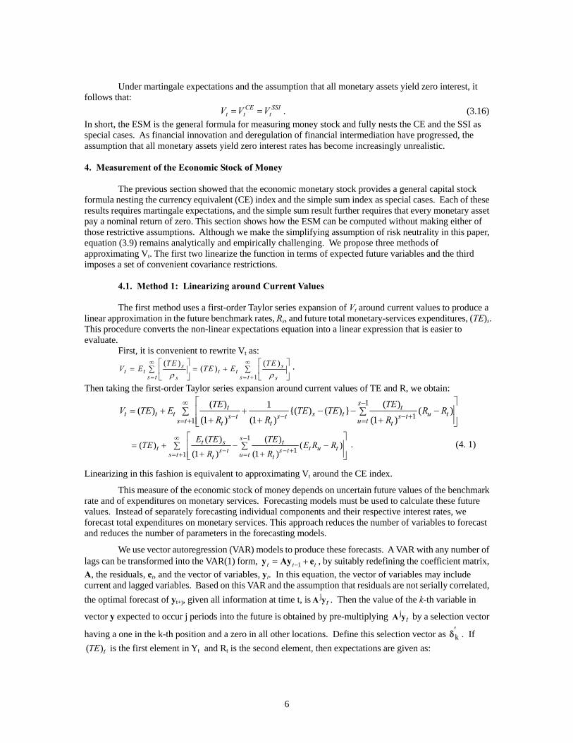
tt VVV ==In short, the ESM is the general formula for measuring money stock and fully nests the CE and the SSI as special cases. As financial innovation and deregulation of financial intermediation have progressed, the assumption that all monetary assets yield zero interest rates has become increasingly unrealistic. 4. Measurement of the Economic Stock of Money The previous section showed that the economic monetary stock provides a general capital stock formula nesting the currency equivalent (CE) index and the simple sum index as special cases. Each of these results requires martingale expectations, and the simple sum result further requires that every monetary asset pay a nominal return of zero. This section shows how the ESM can be computed without making either of those restrictive assumptions. Although we make the simplifying assumption of risk neutrality in this paper, equation (3.9) remains analytically and empirically challenging. We propose three methods of approximating Vt. The first two linearize the function in terms of expected future variables and the third imposes a set of convenient covariance restrictions. 4.1. Method 1: Linearizing around Current Values The first method uses a first-order Taylor series expansion of Vt around current values to produce a linear approximation in the future benchmark rates, Rs, and future total monetary-services expenditures, (TE)s. This procedure converts the non-linear expectations equation into a linear expression that is easier to evaluate. First, it is convenient to rewrite Vt as:
1
( ) ( )( )s s
t t t ts t s ts s
TE TEV E TE E
ρ ρ
∞ ∞
= =
⎡ ⎤ ⎡= = +∑ ∑⎢ ⎥ ⎢
⎣ ⎦ ⎣+
⎤⎥⎦
.
Then taking the first-order Taylor series expansion around current values of TE and R, we obtain:
1
11
( ) ( )1( ) {( ) ( ) } ( )(1 ) (1 ) (1 )
st tt t t s t u ts t s t s ts t u tt t t
TE TEV TE E TE TE R R
R R R
∞ −
− − − += + =
⎡ ⎤= + + − − −⎢ ⎥∑ ∑
+ + +⎢ ⎥⎣ ⎦
1
11
( ) ( ) ( ) ( )
(1 ) (1 )
st s tt s t s ts t u tt t
E TE TETE E R R
R R
∞ −
− − += + =
⎡ ⎤= + − −⎢∑ ∑
+ +⎢ ⎥⎣ ⎦t u t ⎥
t
. (4. 1)
Linearizing in this fashion is equivalent to approximating Vt around the CE index.
This measure of the economic stock of money depends on uncertain future values of the benchmark rate and of expenditures on monetary services. Forecasting models must be used to calculate these future values. Instead of separately forecasting individual components and their respective interest rates, we forecast total expenditures on monetary services. This approach reduces the number of variables to forecast and reduces the number of parameters in the forecasting models.
We use vector autoregression (VAR) models to produce these forecasts. A VAR with any number of lags can be transformed into the VAR(1) form, 1t t−= +y Ay e , by suitably redefining the coefficient matrix, A, the residuals, et, and the vector of variables, yt. In this equation, the vector of variables may include current and lagged variables. Based on this VAR and the assumption that residuals are not serially correlated, the optimal forecast of yt+j, given all information at time t, is . Then the value of the k-th variable in
vector y expected to occur j periods into the future is obtained by pre-multiplying by a selection vector
having a one in the k-th position and a zero in all other locations. Define this selection vector as . If is the first element in Y
jtA y
jtA y
k′δ
( )tTE t and Rt is the second element, then expectations are given as:
6
jt t j 1E [(TE) ]+
′= A yδ t and . These expressions are used to eliminate expectation terms from (4.1). For example, the function of current and expected future monetary expenditures becomes:
jt t j 2 tE R +
′= A Yδ
[( ) ](1 )
t ss ts t t
E TER
∞
−=
⎡ ⎤⎢ ⎥∑
+⎢ ⎥⎣ ⎦1
11
s ts t
ts t tR
−∞ −
=
⎛ ⎞′= ∑ ⎜ ⎟+⎝ ⎠
A yδ (4. 2)
The terms involving the sum of current and expected future benchmark returns are:
11
21 11 1
( ) ( )( ) = (
(1 ) (1 )
ss u tt tt u t t ts t s ts t u t s t u tt t
TE TE)E R R R
R R
−∞ − ∞ −− + − += + = = + =
⎡ ⎤ ′− −∑⎢ ⎥∑ ∑ ∑+ +⎢ ⎥⎣ ⎦
A yδ (4. 3)
Combining results from equations (4.2) and (4.3), we obtain the Method 1 solution for Vt:
1
t 1 211
1V = - ( )1 (1 )
s t ss t u ttt s ts t s t u tt t
TEt tR
R R
− ∞ −∞ −− += = + =
⎛ ⎞′ −∑ ∑ ∑⎜ ⎟+ +⎝ ⎠
A y A yδ −′δ . (4. 4)
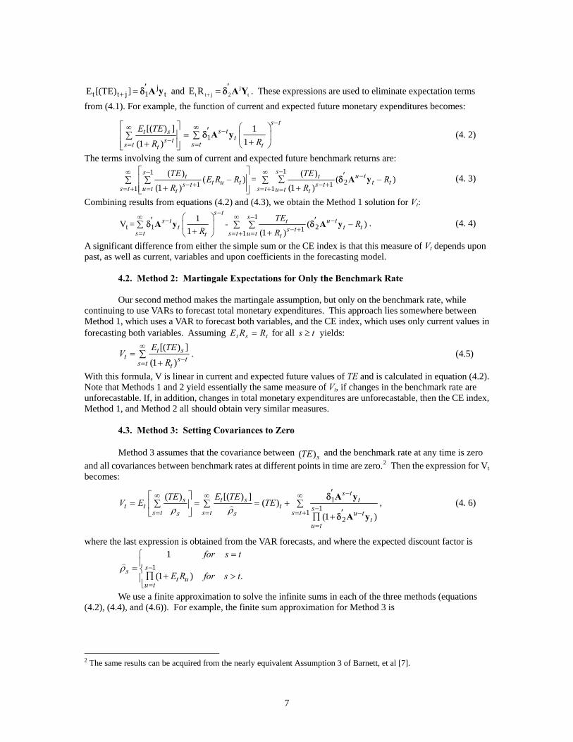
A significant difference from either the simple sum or the CE index is that this measure of Vt depends upon past, as well as current, variables and upon coefficients in the forecasting model. 4.2. Method 2: Martingale Expectations for Only the Benchmark Rate Our second method makes the martingale assumption, but only on the benchmark rate, while continuing to use VARs to forecast total monetary expenditures. This approach lies somewhere between Method 1, which uses a VAR to forecast both variables, and the CE index, which uses only current values in forecasting both variables. Assuming tst RRE = for all s t≥ yields:
[( ) ]
(1 )t s
t s ts t t
E TEV
R
∞
−== ∑
+. (4.5)
With this formula, V is linear in current and expected future values of TE and is calculated in equation (4.2). Note that Methods 1 and 2 yield essentially the same measure of Vt, if changes in the benchmark rate are unforecastable. If, in addition, changes in total monetary expenditures are unforecastable, then the CE index, Method 1, and Method 2 all should obtain very similar measures. 4.3. Method 3: Setting Covariances to Zero Method 3 assumes that the covariance between ( )sTE and the benchmark rate at any time is zero and all covariances between benchmark rates at different points in time are zero.2 Then the expression for Vt becomes:
111
2
( ) [( ) ]( )
(1 )
s ts t s t
t t t ss t s t s t u ts st
u t
TE E TEV E TE
ρ ρ
−∞ ∞ ∞
−= = = + −
=
′⎡ ⎤= = = +∑ ∑ ∑⎢ ⎥
′⎣ ⎦ ∏ +
A y
A y
δ
δ, (4. 6)
where the last expression is obtained from the VAR forecasts, and where the expected discount factor is
1
1
(1 ) .ss
t uu t
for s t
E R for s tρ −
=
=⎧⎪= ⎨∏ + >⎪
⎩
We use a finite approximation to solve the infinite sums in each of the three methods (equations (4.2), (4.4), and (4.6)). For example, the finite sum approximation for Method 3 is
2 The same results can be acquired from the nearly equivalent Assumption 3 of Barnett, et al [7].
7

[( ) ]
( )J t s
ts t s
E TEV J
ρ=
⎡ ⎤= ∑⎢⎣ ⎦
⎥ (4.7)
for any value of J > t. Taking the limit as J goes to infinity in equation (4.7) yields equation (4.6). Having expectations in the numerator and denominator rules out a simple closed-form solution.3 An alternative way of writing equation (4.7) is
[( ) ]
( ) ( 1) t Jt t
J
E TEV J V J
ρ= − + . (4. 8)
Starting with Vt(0)=(TE)t, this equation builds up the measure of Vt recursively. Our approach is to let J increase until we get the convergence, ( ) ( 1) 0t tV J V J− − → , with the convergence criterion
7( ) ( 1)10
( 1)t t
t
V J V JV J
−− −<
−. (4.9)
5. Forecasting Models To construct the forecasts needed for calculating each approximation to the ESM, we consider three types of vector autoregressions: unrestricted , asymmetric, and Bayesian VAR. Because of Bayesian VAR models’ prior degree of success in forecasting economic data, we emphasize those results within the body of the paper, and provide results with the other two approaches in footnotes. Since robustness across forecasting methods is our primary result, rather than our advocacy of any particular forecasting model, we do view the unrestricted and asymmetric VAR results to be relevant to understanding the findings of this paper. 5.1. Unrestricted VARs The unrestricted vector autoregressive model (UVAR) pioneered by Sims [19] is a standard model in the literature. Sims developed the VAR approach as a tool for allowing historical data to summarize the dynamic interactions among time series variables. A hallmark feature of any UVAR is that it has the same number of lags of each variable in each equation. UVARs tend to obtain a relatively large number of statistically insignificant coefficients. As a result, there are concerns about forecasting with UVAR models. Various approaches exist for solving this overparameterization problem. 5.2. Asymmetric VARs One way to reduce the number of parameters in the VAR is to eliminate the common lag assumption. Keating ([13], [14]), for example, developed the asymmetric VAR (AVAR), which is a VAR allowing lag lengths to vary across variables in the model. The AVAR and UVAR models share a common trait: each equation in the model has exactly the same set of explanatory variables without cross equation restrictions. Consequently, AVARs and UVARs are consistently and efficiently estimated by ordinary least squares under standard regularity conditions. However, an AVAR model is expected to have fewer insignificant coefficients, and thereby may obtain smaller out-of-sample forecast errors than the UVAR. An AVAR lag specification can be chosen by an information criterion or by any other methods capable of testing non-nested alternatives. 5.3. Bayesian VARs Another response to overparameterization in UVAR models is the Bayesian approach of Doan, et al [11] and Litterman [15]. A Bayesian VAR (BVAR) model avoids exclusion restrictions, such as the different lag lengths permitted under the AVAR approach. Instead, BVAR models assume each VAR coefficient is
3 Note that we can obtain closed-form expressions for Methods 1 and 2, if all roots of A/(1 + Rt) are outside the unit circle. The finite approximations to infinite sums in the paper also require that condition on roots. These finite approximations will be nearly the same as the closed form solutions, because the convergence criterion, equation (4.9), is very small.
8
drawn from a normal distribution and impose restrictions on the mean and the variance of each of those distributions. The Minnesota (or Litterman) prior is based on the empirical evidence that most economic variables appear to have a unit root. Thus each coefficient is given a prior mean of zero, except for the coefficient on the first lag of the dependent variable in each equation. That coefficient has a mean of one. Coefficients on shorter lags are given larger prior variances than the coefficients on longer lags. This choice of prior variances is based on the reasonable assumption that recent data are likely to be more informative than older data in explaining current outcomes, so recent data should be permitted to dominate prior views about short lag parameters. This approach also allows different priors to be imposed on different variables. For example, if a certain variable is thought to have more explanatory power than other variables, the prior variance associated with that variable would be made larger than for the other variables to permit the information in the data to dominate the prior. Flat (non-informative) priors are assumed for all deterministic variables. 6. Model Specification 6.1. Data Description The models in this paper use U.S. data for total expenditure on monetary services (TE), the benchmark interest rate (BENCH), industrial production (INDPRO), and the consumer price index (CPI). Relative to the notation in section (2.1), BENCHt = Rt and CPIt = p *
t , although the latter equality is an index number theoretic approximation to the exact true cost of living index of economic theory. Data are monthly and seasonally adjusted, covering the period from 1959:1 through 2004:3. All data were obtained from the Federal Reserve Economic Database (FRED), published by the Federal Reserve Bank of St. Louis.4 The initial choice of output and price was based on a priori beliefs regarding those variables most likely to help forecast interest rates and monetary-services expenditures. Those prior beliefs were then supported by statistical tests for marginal predictive content. We also considered other variables in the specification search, but those additional variables did not improve the forecasts and are therefore omitted from the final equations. The choice of benchmark rate can have important consequences for the ESM or the CE index. Rotemberg, et al [17] used the commercial paper rate and found that their CE index was extremely volatile. Our benchmark rate path is the upper envelope over the paths of Moody's BAA bond rate and the interest rates of all of the components of the Federal Reserve’s broadest aggregate. The resulting benchmark rate is not as volatile as the commercial paper rate. In each VAR , we control for the effects of exogenous oil supply shocks by including dummy variables for oil shock dates. We used the dates identified by Hoover, et al [12].5 To model the dynamic response of the economy to oil price shocks, the VAR included current and seven lags of the oil shock dummy variables. To appropriately specify the forecasting models, we needed answers to several important questions. Are the data nonstationary? How many lags should the VAR models have? What values should be given to the hyperparameters that are used in constructing priors in the BVAR approach? 6.2. Nonstationarity and Data Transformation We use standard unit root tests to answer questions about stationarity. Table 1 reports ρ-test results from augmented Dickey-Fuller regressions along with results from Phillips-Perron (PP) Z-tests.
4 At each level of aggregation, j, total expenditure on the monetary services, ( ) j
tTE , was computed from the first equality in equation (3.6). The data source details and the list of monetary assets included at each level of aggregation can be found in [6], which contains the details of the design and data, but not the empirical results that are in this paper. 5 Hoover and Perez’s (1994) shock dates are 1969:3, 1970:12, 1974:1, 1978:3, 1979:9, and 1981:2.
9
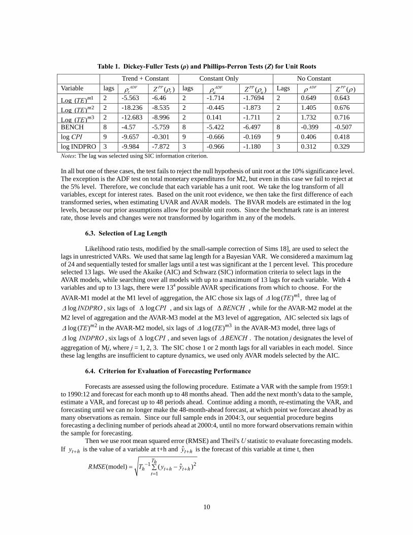
Table 1. Dickey-Fuller Tests (ρ) and Phillips-Perron Tests (Z) for Unit Roots
Trend + Constant Constant Only No Constant Variable lags ADF
τρ ( )PPZ τρ lags ADFμρ ( )PPZ μρ Lags ADFρ ( )PPZ ρ
Log 1( )mTE 2 -5.563 -6.46 2 -1.714 -1.7694 2 0.649 0.643
Log 2( )mTE 2 -18.236 -8.535 2 -0.445 -1.873 2 1.405 0.676
Log 3( )mTE 2 -12.683 -8.996 2 0.141 -1.711 2 1.732 0.716 BENCH 8 -4.57 -5.759 8 -5.422 -6.497 8 -0.399 -0.507 log CPI 9 -9.657 -0.301 9 -0.666 -0.169 9 0.406 0.418 log INDPRO 3 -9.984 -7.872 3 -0.966 -1.180 3 0.312 0.329 Notes: The lag was selected using SIC information criterion. In all but one of these cases, the test fails to reject the null hypothesis of unit root at the 10% significance level. The exception is the ADF test on total monetary expenditures for M2, but even in this case we fail to reject at the 5% level. Therefore, we conclude that each variable has a unit root. We take the log transform of all variables, except for interest rates. Based on the unit root evidence, we then take the first difference of each transformed series, when estimating UVAR and AVAR models. The BVAR models are estimated in the log levels, because our prior assumptions allow for possible unit roots. Since the benchmark rate is an interest rate, those levels and changes were not transformed by logarithm in any of the models. 6.3. Selection of Lag Length Likelihood ratio tests, modified by the small-sample correction of Sims 18], are used to select the lags in unrestricted VARs. We used that same lag length for a Bayesian VAR. We considered a maximum lag of 24 and sequentially tested for smaller lags until a test was significant at the 1 percent level. This procedure selected 13 lags. We used the Akaike (AIC) and Schwarz (SIC) information criteria to select lags in the AVAR models, while searching over all models with up to a maximum of 13 lags for each variable. With 4 variables and up to 13 lags, there were 134 possible AVAR specifications from which to choose. For the AVAR-M1 model at the M1 level of aggregation, the AIC chose six lags of three lag of 1log ( ) ,mTEΔ
log INDPROΔ , six lags of , and six lags of CPIlogΔ BENCHΔ , while for the AVAR-M2 model at the M2 level of aggregation and the AVAR-M3 model at the M3 level of aggregation, AIC selected six lags of
in the AVAR-M2 model, six lags of in the AVAR-M3 model, three lags of 2log ( )mTEΔ 3log ( )mTEΔlog INDPROΔ , six lags of , and seven lags of CPIlogΔ BENCHΔ . The notation j designates the level of
aggregation of Mj, where j = 1, 2, 3. The SIC chose 1 or 2 month lags for all variables in each model. Since these lag lengths are insufficient to capture dynamics, we used only AVAR models selected by the AIC. 6.4. Criterion for Evaluation of Forecasting Performance Forecasts are assessed using the following procedure. Estimate a VAR with the sample from 1959:1 to 1990:12 and forecast for each month up to 48 months ahead. Then add the next month’s data to the sample, estimate a VAR, and forecast up to 48 periods ahead. Continue adding a month, re-estimating the VAR, and forecasting until we can no longer make the 48-month-ahead forecast, at which point we forecast ahead by as many observations as remain. Since our full sample ends in 2004:3, our sequential procedure begins forecasting a declining number of periods ahead at 2000:4, until no more forward observations remain within the sample for forecasting. Then we use root mean squared error (RMSE) and Theil's U statistic to evaluate forecasting models. If is the value of a variable at t+h and t hy + ˆt hy + is the forecast of this variable at time t, then
1 2
1ˆ (model) ( )
Thh t h t h
tRMSE T y y−
+ +=
= −∑
10
and
2
1
2
1
ˆ( )RMSE (model)
RMSE (random walk)( )
Tht h t h
tTh
t h tt
y yTheil U
y y
+ +=
+=
∑ −= =
∑ −
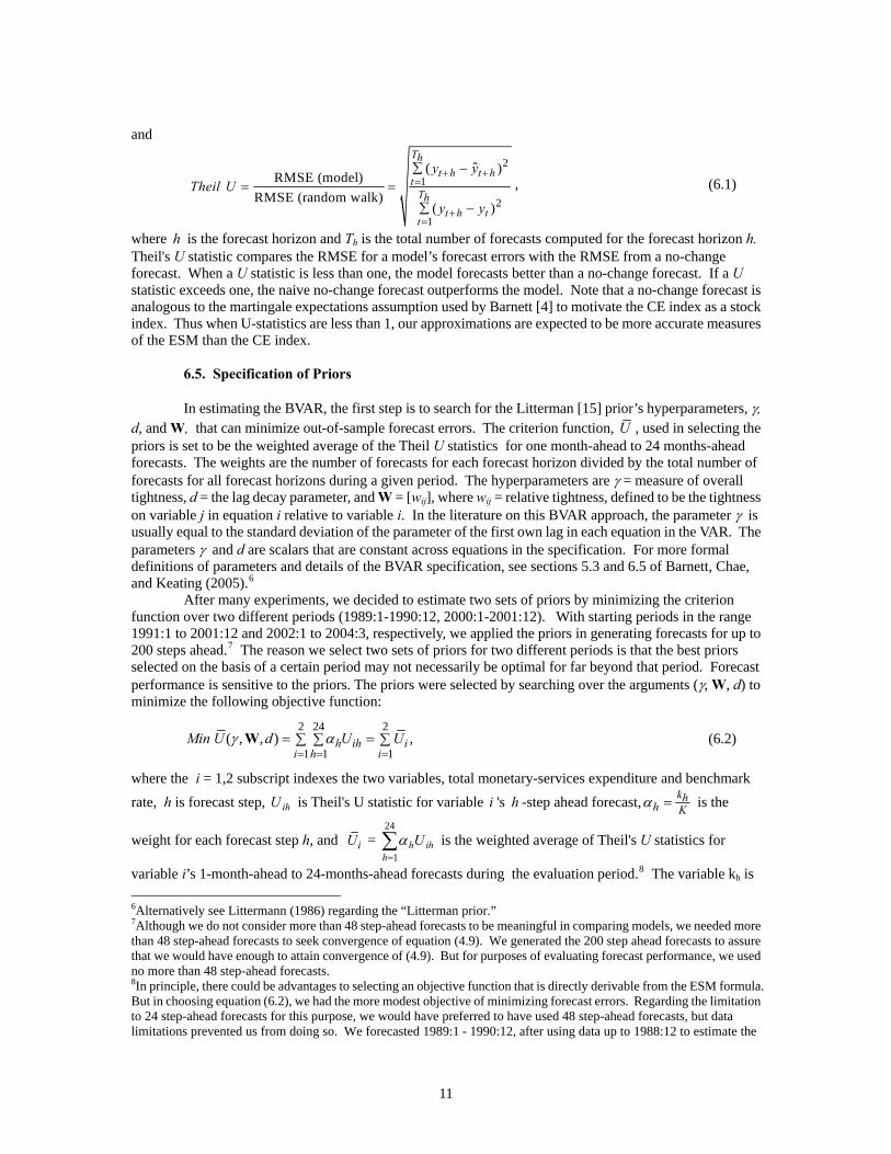
, (6.1)
where is the forecast horizon and Th h is the total number of forecasts computed for the forecast horizon h. Theil's U statistic compares the RMSE for a model’s forecast errors with the RMSE from a no-change forecast. When a U statistic is less than one, the model forecasts better than a no-change forecast. If a U statistic exceeds one, the naive no-change forecast outperforms the model. Note that a no-change forecast is analogous to the martingale expectations assumption used by Barnett [4] to motivate the CE index as a stock index. Thus when U-statistics are less than 1, our approximations are expected to be more accurate measures of the ESM than the CE index. 6.5. Specification of Priors In estimating the BVAR, the first step is to search for the Litterman [15] prior’s hyperparameters, γ, d, and W, that can minimize out-of-sample forecast errors. The criterion function, U , used in selecting the priors is set to be the weighted average of the Theil U statistics for one month-ahead to 24 months-ahead forecasts. The weights are the number of forecasts for each forecast horizon divided by the total number of forecasts for all forecast horizons during a given period. The hyperparameters are γ = measure of overall tightness, d = the lag decay parameter, and W = [wij], where wij = relative tightness, defined to be the tightness on variable j in equation i relative to variable i. In the literature on this BVAR approach, the parameter γ is usually equal to the standard deviation of the parameter of the first own lag in each equation in the VAR. The parameters γ and d are scalars that are constant across equations in the specification. For more formal definitions of parameters and details of the BVAR specification, see sections 5.3 and 6.5 of Barnett, Chae, and Keating (2005).6
After many experiments, we decided to estimate two sets of priors by minimizing the criterion function over two different periods (1989:1-1990:12, 2000:1-2001:12). With starting periods in the range 1991:1 to 2001:12 and 2002:1 to 2004:3, respectively, we applied the priors in generating forecasts for up to 200 steps ahead.7 The reason we select two sets of priors for two different periods is that the best priors selected on the basis of a certain period may not necessarily be optimal for far beyond that period. Forecast performance is sensitive to the priors. The priors were selected by searching over the arguments (γ, W, d) to minimize the following objective function:
2 24 2
1 1 1( , , ) ,h ih i
i h iMin U d U Uγ α
= = == =∑ ∑ ∑W (6.2)
where the i = 1,2 subscript indexes the two variables, total monetary-services expenditure and benchmark rate, h is forecast step, is Theil's U statistic for variable i 's -step ahead forecast,ihU h kh
h Kα = is the
weight for each forecast step h, and iU = is the weighted average of Theil's U statistics for
variable i’s 1-month-ahead to 24-months-ahead forecasts during the evaluation period.
ihhh
Uα∑=
24
18 The variable kh is
6Alternatively see Littermann (1986) regarding the “Litterman prior.” 7Although we do not consider more than 48 step-ahead forecasts to be meaningful in comparing models, we needed more than 48 step-ahead forecasts to seek convergence of equation (4.9). We generated the 200 step ahead forecasts to assure that we would have enough to attain convergence of (4.9). But for purposes of evaluating forecast performance, we used no more than 48 step-ahead forecasts. 8In principle, there could be advantages to selecting an objective function that is directly derivable from the ESM formula. But in choosing equation (6.2), we had the more modest objective of minimizing forecast errors. Regarding the limitation to 24 step-ahead forecasts for this purpose, we would have preferred to have used 48 step-ahead forecasts, but data limitations prevented us from doing so. We forecasted 1989:1 - 1990:12, after using data up to 1988:12 to estimate the
11
the number of times that the h -step ahead forecast has been computed during the evaluation period, and
is the total number of times that all forecasts for 1 to 24 months ahead have been computed during
the evaluation period.
hh
kK24
1=∑=
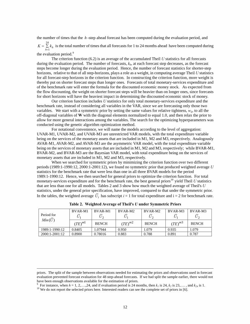
9 The criterion function (6.2) is an average of the accumulated Theil U statistics for all forecasts during the evaluation period. The number of forecasts, kh, at each forecast step decreases, as the forecast steps become longer during the evaluation period. Hence, the number of forecast statistics for shorter-step horizons, relative to that of all step-horizons, plays a role as a weight, in computing average Theil U statistics for all forecast-step horizons in the criterion function. In constructing the criterion function, more weight is thereby put on shorter forecast steps than longer ones. Forecasts of total monetary-services expenditure and of the benchmark rate will enter the formula for the discounted economic money stock. As expected from the flow discounting, the weight on shorter forecast steps will be heavier than on longer ones, since forecasts for short horizons will have the heaviest impact in determining the discounted economic stock of money. Our criterion function includes U statistics for only total monetary-services expenditure and the benchmark rate, instead of considering all variables in the VAR, since we are forecasting only those two variables. We start with a symmetric prior by setting the same values for relative tightness, wij, to all the off-diagonal variables of W with the diagonal elements normalized to equal 1.0, and then relax the prior to allow for more general interactions among the variables. The search for the optimizing hyperparameters was conducted using the genetic algorithm optimization method. For notational convenience, we will name the models according to the level of aggregation: UVAR-M1, UVAR-M2, and UVAR-M3 are unrestricted VAR models, with the total expenditure variable being on the services of the monetary assets that are included in M1, M2 and M3, respectively. Analogously AVAR-M1, AVAR-M2, and AVAR-M3 are the asymmetric VAR model, with the total expenditure variable being on the services of monetary assets that are included in M1, M2 and M3, respectively; while BVAR-M1, BVAR-M2, and BVAR-M3 are the Bayesian VAR model, with total expenditure being on the services of monetary assets that are included in M1, M2 and M3, respectively. When we searched for symmetric priors by minimizing the criterion function over two different periods (1989:1-1990:12, 2000:1-2001:12), we found no symmetric prior that produced weighted average U statistics for the benchmark rate that were less than one in all three BVAR models for the period 1989:1-1990:12. Hence, we then searched for general priors to optimize the criterion function. For total monetary-services expenditure and for the benchmark rate, the best general priors10 yield Theil U statistics that are less than one for all models. Tables 2 and 3 show how much the weighted average of Theil's U statistics, under the general prior specification, have improved, compared to that under the symmetric prior. In the tables, the weighted average iU has subscript i = 1 for total expenditure and i = 2 for benchmark rate.
Table 2. Weighted Average of Theil's U under Symmetric Priors
BVAR-M1 1U
BVAR-M1 2U
BVAR-M2 1U
BVAR-M2 2U
BVAR-M3 1U
BVAR-M3 2U Period for
( )Min U 1( )mTE BENCH 2( )mTE BENCH 3( )mTE BENCH
1989:1-1990:12 0.8405 1.07944 0.950 1.079 0.935 1.079 2000:1-2001:12 0.8900 0.78016 0.883 0.788 0.891 0.787
priors. The split of the sample between observations needed for estimating the priors and observations used in forecast evaluation prevented forecast evaluation for 48 step-ahead forecasts. If we had split the sample earlier, there would not have been enough observations available for the estimation of priors. 9 For instance, when h = 1, 2,….,24, and if evaluation period is 24 months, then k1 is 24, k2 is 23,…. , and k24 is 1. 10 We do not report the selected priors here. Interested readers can see the complete set of priors in [6].
12
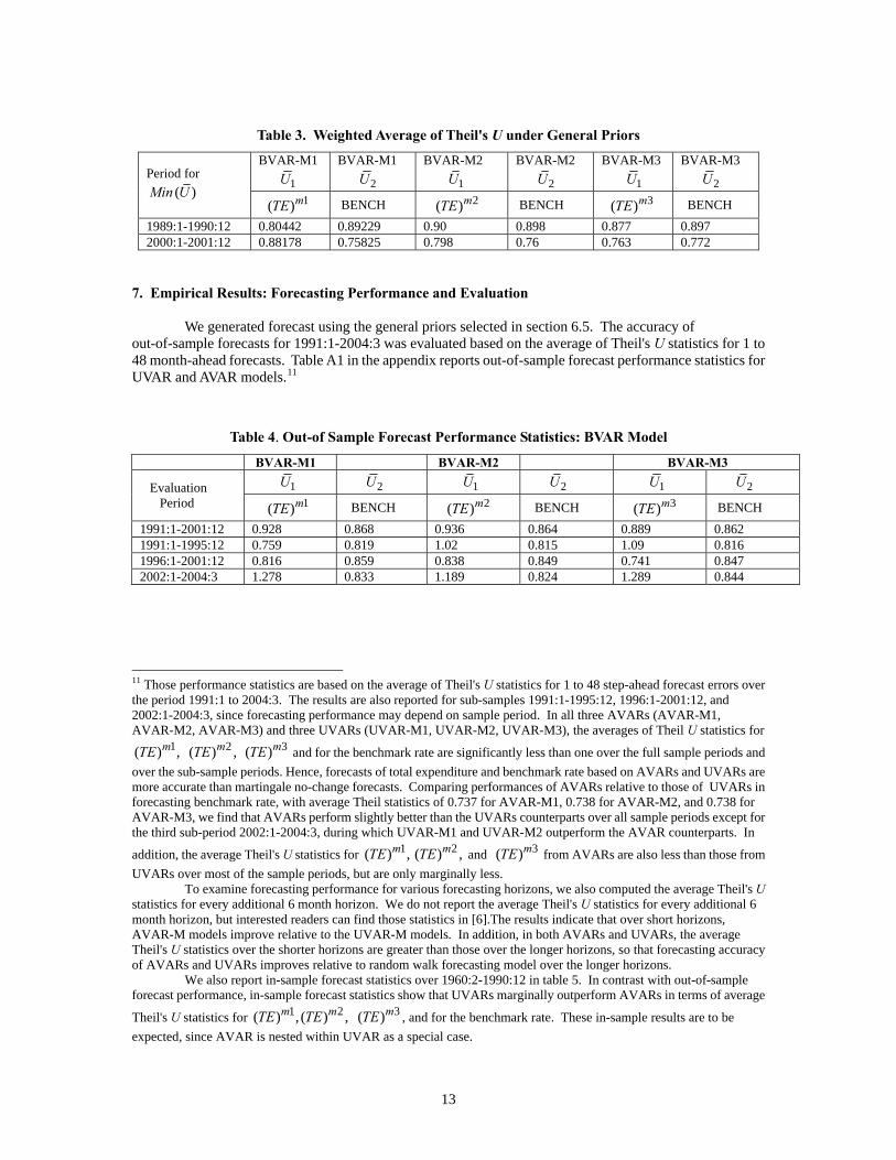
Table 3. Weighted Average of Theil's U under General Priors
BVAR-M1 1U
BVAR-M1 2U
BVAR-M2 1U
BVAR-M2 2U
BVAR-M3 1U
BVAR-M3 2U Period for
( )Min U 1( )mTE BENCH 2( )mTE BENCH 3( )mTE BENCH
1989:1-1990:12 0.80442 0.89229 0.90 0.898 0.877 0.897 2000:1-2001:12 0.88178 0.75825 0.798 0.76 0.763 0.772
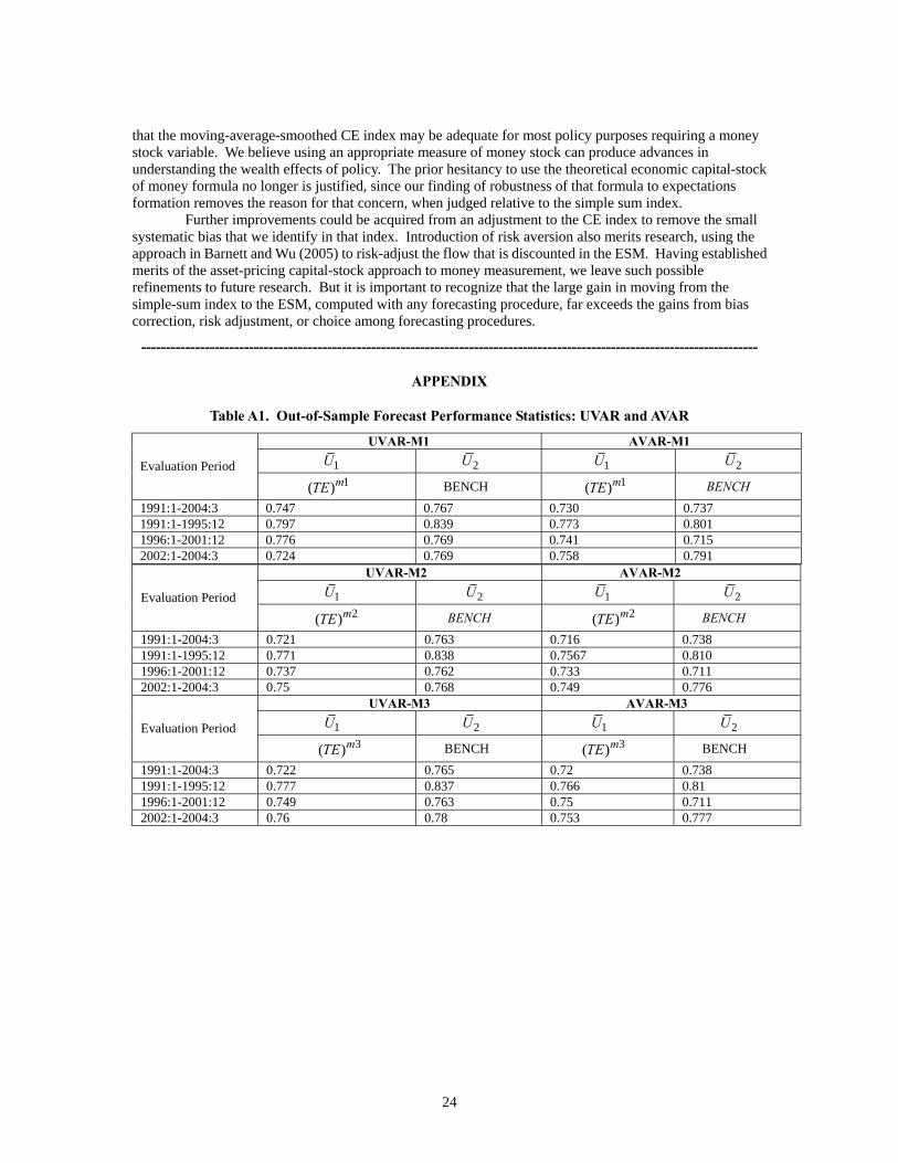
7. Empirical Results: Forecasting Performance and Evaluation We generated forecast using the general priors selected in section 6.5. The accuracy of out-of-sample forecasts for 1991:1-2004:3 was evaluated based on the average of Theil's U statistics for 1 to 48 month-ahead forecasts. Table A1 in the appendix reports out-of-sample forecast performance statistics for UVAR and AVAR models.11
Table 4. Out-of Sample Forecast Performance Statistics: BVAR Model
BVAR-M1 BVAR-M2 BVAR-M3 1U 2U 1U 2U 1U 2U Evaluation
Period 1( )mTE BENCH 2( )mTE BENCH 3( )mTE BENCH 1991:1-2001:12 0.928 0.868 0.936 0.864 0.889 0.862 1991:1-1995:12 0.759 0.819 1.02 0.815 1.09 0.816 1996:1-2001:12 0.816 0.859 0.838 0.849 0.741 0.847 2002:1-2004:3 1.278 0.833 1.189 0.824 1.289 0.844
m mTE TE
11 Those performance statistics are based on the average of Theil's U statistics for 1 to 48 step-ahead forecast errors over the period 1991:1 to 2004:3. The results are also reported for sub-samples 1991:1-1995:12, 1996:1-2001:12, and 2002:1-2004:3, since forecasting performance may depend on sample period. In all three AVARs (AVAR-M1, AVAR-M2, AVAR-M3) and three UVARs (UVAR-M1, UVAR-M2, UVAR-M3), the averages of Theil U statistics for
and for the benchmark rate are significantly less than one over the full sample periods and over the sub-sample periods. Hence, forecasts of total expenditure and benchmark rate based on AVARs and UVARs are more accurate than martingale no-change forecasts. Comparing performances of AVARs relative to those of UVARs in forecasting benchmark rate, with average Theil statistics of 0.737 for AVAR-M1, 0.738 for AVAR-M2, and 0.738 for AVAR-M3, we find that AVARs perform slightly better than the UVARs counterparts over all sample periods except for the third sub-period 2002:1-2004:3, during which UVAR-M1 and UVAR-M2 outperform the AVAR counterparts. In
addition, the average Theil's U statistics for , and from AVARs are also less than those from UVARs over most of the sample periods, but are only marginally less. To examine forecasting performance for various forecasting horizons, we also computed the average Theil's U statistics for every additional 6 month horizon. We do not report the average Theil's U statistics for every additional 6 month horizon, but interested readers can find those statistics in [6].The results indicate that over short horizons, AVAR-M models improve relative to the UVAR-M models. In addition, in both AVARs and UVARs, the average Theil's U statistics over the shorter horizons are greater than those over the longer horizons, so that forecasting accuracy of AVARs and UVARs improves relative to random walk forecasting model over the longer horizons.
1( ) ,mTE 2( ) ,mTE 3( )mTE
1 2( ) , ( ) 3( )mTE
We also report in-sample forecast statistics over 1960:2-1990:12 in table 5. In contrast with out-of-sample forecast performance, in-sample forecast statistics show that UVARs marginally outperform AVARs in terms of average
Theil's U statistics for , and for the benchmark rate. These in-sample results are to be expected, since AVAR is nested within UVAR as a special case.
1 2( ) , ( ) ,m mTE TE 3( )mTE
13
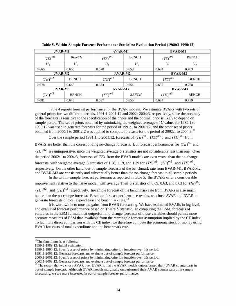
Table 5. Within-Sample Forecast Performance Statistics: Evaluation Period (1960:2-1990:12)
UVAR-M1 AVAR-M1 BVAR-M1
(TE) m1 BENCH (TE) m1 BENCH (TE) m1 BENCH
1U 2U 1U 2U 1U 2U 0.665 0.650 0.670 0.658 0.694 0.763 UVAR-M2 AVAR-M2 BVAR-M2
2( )mTE BENCH 2( )mTE BENCH 2( )mTE BENCH 0.678 0.648 0.684 0.654 0.637 0.758 UVAR-M3 AVAR-M3 BVAR-M3
3( )mTE BENCH 3( )mTE BENCH 3( )mTE BENCH 0.681 0.648 0.687 0.655 0.634 0.759
Table 4 reports forecast performance for the BVAR models. We estimate BVARs with two sets of general priors for two different periods, 1991:1-2001:12 and 2002:-2004:3, respectively, since the accuracy of the forecasts is sensitive to the specification of the priors and the optimal prior is likely to depend on sample period. The set of priors obtained by minimizing the weighted average of U values for 1989:1 to 1990:12 was used to generate forecasts for the period of 1991:1 to 2001:12, and the other set of priors obtained from 2000:1 to 2001:12 was applied to compute forecasts for the period of 2002:1 to 2004:3.12
Over the sample period 1991:1 to 2001:12, forecasts of , and from
BVARs are better than the corresponding no-change forecasts. But forecast performances for and
are unimpressive, since the weighted average U statistics are not considerably less than one. Over the period 2002:1 to 2004:3, forecasts of from the BVAR models are even worse than the no-change forecasts, with weighted average U statistics of 1.28, 1.19, and 1.29 for and , respectively. On the other hand, out-of sample forecasts of the benchmark rate from BVAR-M1, BVAR-M2, and BVAR-M3 are consistently and substantially better than the no-change forecast in all sample periods.
1( ) ,mTE 2( )mTE 3( )mTE1( )mTE
2( )mTETEs
1( ) ,mTE 2( )mTE ,
3( )mTE
In the within-sample forecast performances reported in table 5, the BVARs offer a considerable improvement relative to the naive model, with average Theil U statistics of 0.69, 0.63, and 0.63 for
, and respectively. In-sample forecast of the benchmark rate from BVARs is also much better than the no-change forecast. Based on forecast performance results, we chose AVAR and BVAR to generate forecasts of total expenditure and benchmark rate.
1( ) ,mTE2( )mTE 3( )mTE
13 It is worthwhile to note the gains from BVAR forecasting. We have estimated BVARs in log level, and evaluated forecast performance based on Theil's U statistic. In computing the ESM, forecasts of variables in the ESM formula that outperform no-change forecasts of those variables should permit more accurate measures of ESM than available from the martingale forecast assumption implied by the CE index. To facilitate direct comparison with the CE index, we therefore compute the economic stock of money using BVAR forecasts of total expenditure and the benchmark rate.
12The time frame is as follows: 1959:1-1988:12: Initial estimation 1989:1-1990:12: Specify a set of priors by minimizing criterion function over this period. 1991:1-2001:12: Generate forecasts and evaluate out-of-sample forecast performance. 2000:1-2001:12: Specify a set of priors by minimizing criterion function over this period. 2002:1-2003:12: Generate forecasts and evaluate out-of-sample forecast performance. 13 The reason that we chose AVAR over UVAR is that the AVAR models outperformed their UVAR counterparts in out-of-sample forecast. Although UVAR models marginally outperformed their AVAR counterparts at in-sample forecasting, we are more interested in out-of-sample forecast performance.
14
8. Empirical Results: Estimation of Money Stock 8.1. Economic Stock of Money Computed using Actual Data
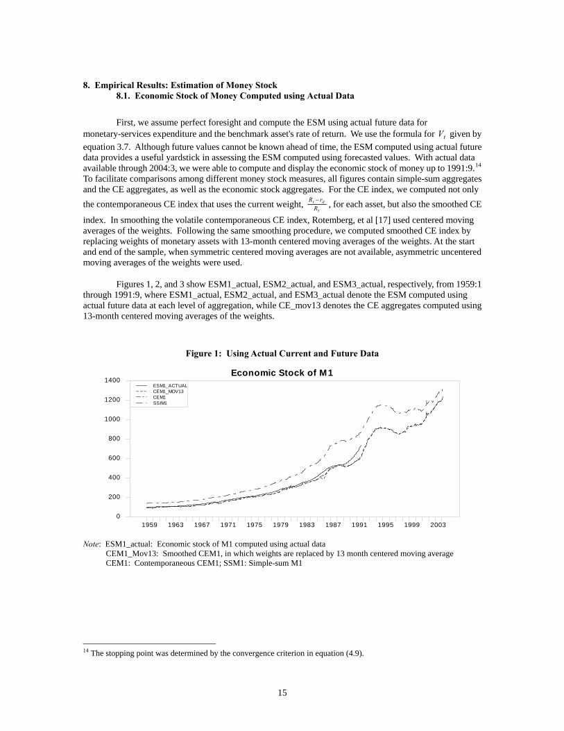
First, we assume perfect foresight and compute the ESM using actual future data for monetary-services expenditure and the benchmark asset's rate of return. We use the formula for given by equation 3.7. Although future values cannot be known ahead of time, the ESM computed using actual future data provides a useful yardstick in assessing the ESM computed using forecasted values. With actual data available through 2004:3, we were able to compute and display the economic stock of money up to 1991:9.
tV
14 To facilitate comparisons among different money stock measures, all figures contain simple-sum aggregates and the CE aggregates, as well as the economic stock aggregates. For the CE index, we computed not only the contemporaneous CE index that uses the current weight,
t
ittR
rR − , for each asset, but also the smoothed CE
index. In smoothing the volatile contemporaneous CE index, Rotemberg, et al [17] used centered moving averages of the weights. Following the same smoothing procedure, we computed smoothed CE index by replacing weights of monetary assets with 13-month centered moving averages of the weights. At the start and end of the sample, when symmetric centered moving averages are not available, asymmetric uncentered moving averages of the weights were used.
Figures 1, 2, and 3 show ESM1_actual, ESM2_actual, and ESM3_actual, respectively, from 1959:1 through 1991:9, where ESM1_actual, ESM2_actual, and ESM3_actual denote the ESM computed using actual future data at each level of aggregation, while CE_mov13 denotes the CE aggregates computed using 13-month centered moving averages of the weights.
Figure 1: Using Actual Current and Future Data
Economic Stock of M1
1959 1963 1967 1971 1975 1979 1983 1987 1991 1995 1999 20030
200
400
600
800
1000
1200
1400ESM1_ACTUALCEM1_MOV13CEM1SSIM1
Note: ESM1_actual: Economic stock of M1 computed using actual data CEM1_Mov13: Smoothed CEM1, in which weights are replaced by 13 month centered moving average CEM1: Contemporaneous CEM1; SSM1: Simple-sum M1
14 The stopping point was determined by the convergence criterion in equation (4.9).
15
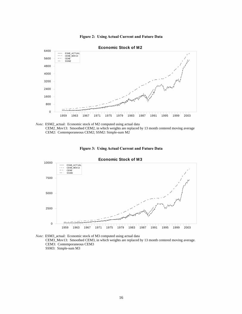
Figure 2: Using Actual Current and Future Data
Economic Stock of M2
1959 1963 1967 1971 1975 1979 1983 1987 1991 1995 1999 20030
800
1600
2400
3200
4000
4800
5600
6400ESM2_ACTUALCEM2_MOV13CEM2SSIM2
Note: ESM2_actual: Economic stock of M2 computed using actual data CEM2_Mov13: Smoothed CEM2, in which weights are replaced by 13 month centered moving average CEM2: Contemporaneous CEM2; SSM2: Simple-sum M2
Figure 3: Using Actual Current and Future Data
Economic Stock of M3
1959 1963 1967 1971 1975 1979 1983 1987 1991 1995 1999 20030
2500
5000
7500
10000ESM3_ACTUALCEM3_MOV13CEM3SSIM3
Note: ESM3_actual: Economic stock of M3 computed using actual data CEM3_Mov13: Smoothed CEM3, in which weights are replaced by 13 month centered moving average. CEM3: Contemporaneous CEM3 SSM3: Simple-sum M3
16
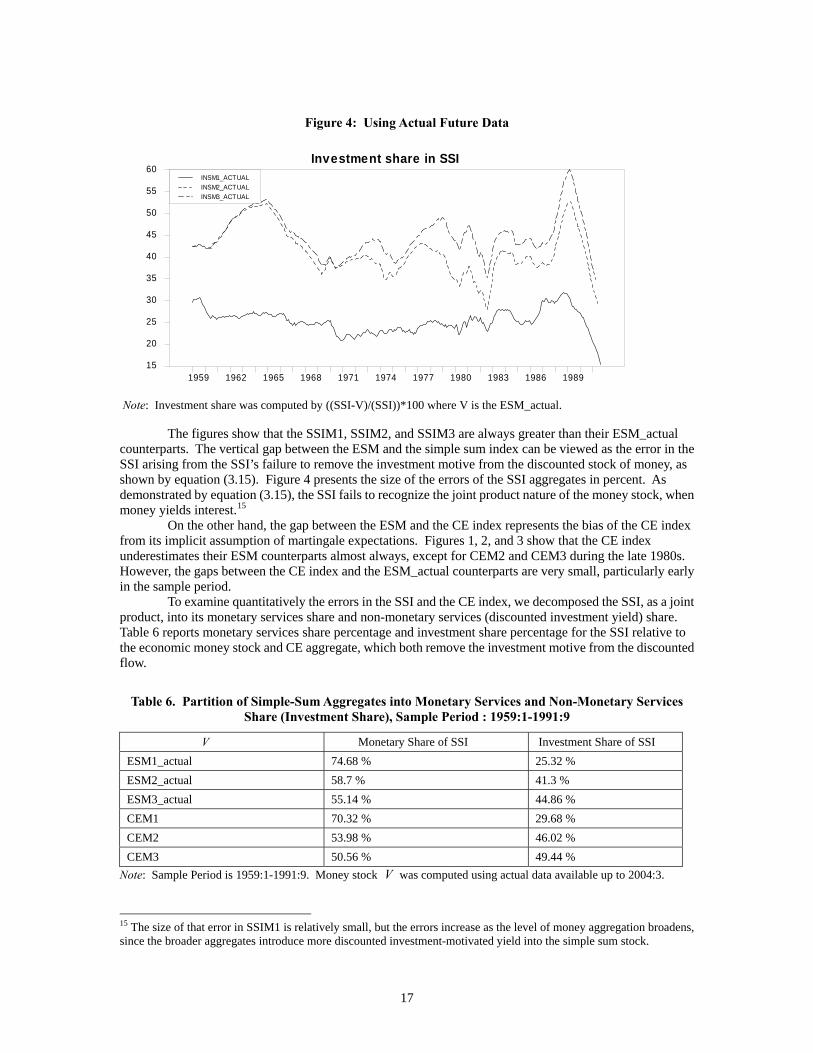
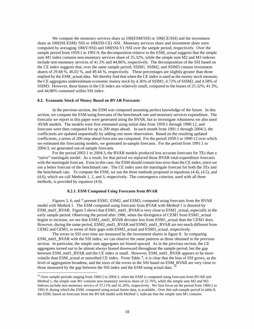
Figure 4: Using Actual Future Data
Investment share in SSI
1959 1962 1965 1968 1971 1974 1977 1980 1983 1986 198915
20
25
30
35
40
45
50
55
60INSM1_ACTUALINSM2_ACTUALINSM3_ACTUAL
Note: Investment share was computed by ((SSI-V)/(SSI))*100 where V is the ESM_actual. The figures show that the SSIM1, SSIM2, and SSIM3 are always greater than their ESM_actual counterparts. The vertical gap between the ESM and the simple sum index can be viewed as the error in the SSI arising from the SSI’s failure to remove the investment motive from the discounted stock of money, as shown by equation (3.15). Figure 4 presents the size of the errors of the SSI aggregates in percent. As demonstrated by equation (3.15), the SSI fails to recognize the joint product nature of the money stock, when money yields interest.15
On the other hand, the gap between the ESM and the CE index represents the bias of the CE index from its implicit assumption of martingale expectations. Figures 1, 2, and 3 show that the CE index underestimates their ESM counterparts almost always, except for CEM2 and CEM3 during the late 1980s. However, the gaps between the CE index and the ESM_actual counterparts are very small, particularly early in the sample period. To examine quantitatively the errors in the SSI and the CE index, we decomposed the SSI, as a joint product, into its monetary services share and non-monetary services (discounted investment yield) share. Table 6 reports monetary services share percentage and investment share percentage for the SSI relative to the economic money stock and CE aggregate, which both remove the investment motive from the discounted flow.
Table 6. Partition of Simple-Sum Aggregates into Monetary Services and Non-Monetary Services
Share (Investment Share), Sample Period : 1959:1-1991:9
V Monetary Share of SSI Investment Share of SSI ESM1_actual 74.68 % 25.32 % ESM2_actual 58.7 % 41.3 % ESM3_actual 55.14 % 44.86 % CEM1 70.32 % 29.68 % CEM2 53.98 % 46.02 % CEM3 50.56 % 49.44 %
Note: Sample Period is 1959:1-1991:9. Money stock V was computed using actual data available up to 2004:3.
15 The size of that error in SSIM1 is relatively small, but the errors increase as the level of money aggregation broadens, since the broader aggregates introduce more discounted investment-motivated yield into the simple sum stock.
17
We compute the monetary services share as 100(ESM/SSI) or 100(CE/SSI) and the investment share as 100(SSI-ESM) /SSI or 100(SSI-CE) /SSI. Monetary services share and investment share were computed by averaging 100(V/SSI) and 100(SSI-V) /SSI over the sample period, respectively. Over the sample period from 1959:1 to 1991:9, the decomposition relative to the ESM_actual suggests that the simple sum M1 index contains non-monetary services share of 25.32%, while the simple sum M2 and M3 indexes include non-monetary services of 41.3% and 44.86%, respectively. The decomposition of the SSI based on the CE index suggests that, over the same sample period, SSIM1, SSIM2, and SSIM3 contain investment shares of 29.68 %, 46.02 %, and 49.44 %, respectively. These percentages are slightly greater than those implied by the ESM_actual data. We thereby find that when the CE index is used as the money stock measure, the CE aggregates underestimate economic money stock by 4.36% of SSIM1, 4.72% of SSIM2, and 4.58% of SSIM3. However, these biases in the CE index are relatively small, compared to the biases of 25.32%, 41.3%, and 44.86% contained within SSI index. 8.2. Economic Stock of Money Based on BVAR Forecasts In the previous section, the ESM was computed assuming perfect knowledge of the future. In this section, we compute the ESM using forecasts of the benchmark rate and monetary-services expenditure. The forecasts we report in this paper were generated using the BVAR, but to investigate robustness we also used AVAR models. The models were first estimated using initial data from 1959:1 through 1990:12, and forecasts were then computed for up to 200 steps ahead. In each month from 1991:1 through 2004:3, the coefficients are updated sequentially by adding one more observation. Based on the resulting updated coefficients, a series of 200-step-ahead forecasts are computed. For the period 1959:1 to 1990:12 over which we estimated the forecasting models, we generated in-sample forecasts. For the period from 1991:1 to 2004:3, we generated out-of-sample forecasts. For the period 2002:1 to 2004:3, the BVAR models produced less accurate forecasts for TEs than a “naive” martingale model. As a result, for that period we replaced those BVAR total-expenditure forecasts with the martingale forecast. Even in this case, the ESM should contain less error than the CE index, since we use a better forecast of the benchmark rate. The CE index uses the martingale forecast for both the TEs and the benchmark rate. To compute the ESM, we use the three methods proposed in equations (4.4), (4.5), and (4.6), which we call Methods 1, 2, and 3, respectively. The convergence criterion, used with all three methods, is provided by equation (4.9). 8.2.1. ESM Computed Using Forecasts from BVAR Figures 5, 6, and 7 present ESM1, ESM2, and ESM3, computed using forecasts from the BVAR model with Method 1. The ESM computed using forecasts from BVAR with Method 1 is denoted by ESM_mtd1_BVAR. Figure 5 shows that ESM1_mtd1_BVAR is very close to ESM1_actual, especially in the early sample period. Observing the period after 1980, when the divergence of CEM1 from ESM1_actual begins to increase, we see that ESM1_mtd1_BVAR deviates less from ESM1_actual than the CEM1 does. However, during the same period, ESM2_mtd1_BVAR and ESM3_mtd1_BVAR are not much different from CEM2 and CEM3, in terms of their gaps with ESM2_actual and ESM3_actual, respectively. The errors in SSI over time are measured by the investment shares in figure 8. In comparing ESM_mtd1_BVAR with the SSI index, we can observe the same patterns as those obtained in the previous section. In particular, the simple sum aggregates are biased upward. As in the previous section, the CE aggregates turned out to be almost always biased downward throughout the sample period, but the gap between ESM_mtd1_BVAR and the CE index is small. However, ESM_mtd1_BVAR appears to be more volatile than ESM_actual or smoothed CE index. From Table 7, it is clear that the bias of SSI grows, as the level of aggregation broadens, and the sizes of the errors in the SSI based on ESM_BVAR are very close to those measured by the gap between the SSI index and the ESM using actual data .16
16 Over sample periods ranging from 1960:2 to 2004:3, when the ESM is computed using forecasts from BVAR and Method 1, the simple sum M1 contains non-monetary services share of 22.76%, while the simple sum M2 and M3 indexes include non-monetary service of 37.11% and 41.26%, respectively. We first focus on the period from 1960:2 to 1991:9, during which the ESM, computed using actual future data, is available. Over this sub-sample period in table 8, the ESM, based on forecasts from the BVAR model with Method 1, indicate that the simple sum M1 contains
18
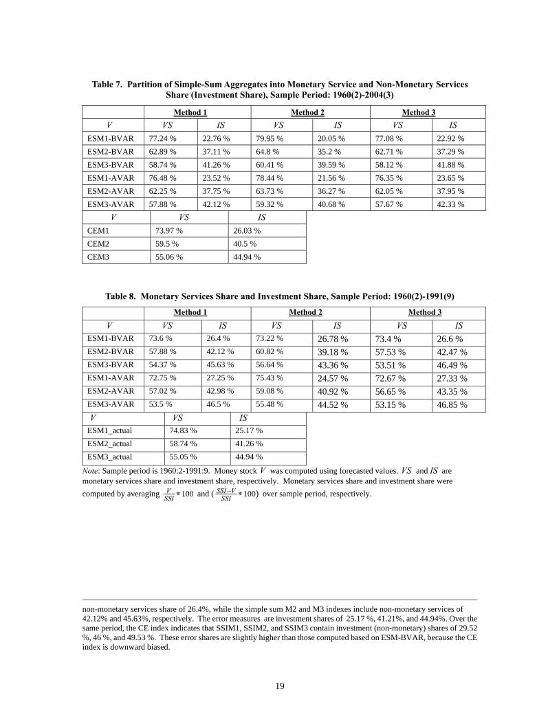
Table 7. Partition of Simple-Sum Aggregates into Monetary Service and Non-Monetary Services Share (Investment Share), Sample Period: 1960(2)-2004(3)
Method 1 Method 2 Method 3 V VS IS VS IS VS ISESM1-BVAR 77.24 % 22.76 % 79.95 % 20.05 % 77.08 % 22.92 % ESM2-BVAR 62.89 % 37.11 % 64.8 % 35.2 % 62.71 % 37.29 % ESM3-BVAR 58.74 % 41.26 % 60.41 % 39.59 % 58.12 % 41.88 % ESM1-AVAR 76.48 % 23.52 % 78.44 % 21.56 % 76.35 % 23.65 % ESM2-AVAR 62.25 % 37.75 % 63.73 % 36.27 % 62.05 % 37.95 % ESM3-AVAR 57.88 % 42.12 % 59.32 % 40.68 % 57.67 % 42.33 % V VS ISCEM1 73.97 % 26.03 % CEM2 59.5 % 40.5 % CEM3 55.06 % 44.94 %
Table 8. Monetary Services Share and Investment Share, Sample Period: 1960(2)-1991(9)
Method 1 Method 2 Method 3
V VS IS VS IS VS ISESM1-BVAR 73.6 % 26.4 % 73.22 % 26.78 % 73.4 % 26.6 % ESM2-BVAR 57.88 % 42.12 % 60.82 % 39.18 % 57.53 % 42.47 % ESM3-BVAR 54.37 % 45.63 % 56.64 % 43.36 % 53.51 % 46.49 % ESM1-AVAR 72.75 % 27.25 % 75.43 % 24.57 % 72.67 % 27.33 % ESM2-AVAR 57.02 % 42.98 % 59.08 % 40.92 % 56.65 % 43.35 % ESM3-AVAR 53.5 % 46.5 % 55.48 % 44.52 % 53.15 % 46.85 % V VS ISESM1_actual 74.83 % 25.17 % ESM2_actual 58.74 % 41.26 % ESM3_actual 55.05 % 44.94 %
Note: Sample period is 1960:2-1991:9. Money stock V was computed using forecasted values. VS and are monetary services share and investment share, respectively. Monetary services share and investment share were computed by averaging
IS
100VSSI ∗ and ( 100)SSI V
SSI− ∗
over sample period, respectively.
non-monetary services share of 26.4%, while the simple sum M2 and M3 indexes include non-monetary services of 42.12% and 45.63%, respectively. The error measures are investment shares of 25.17 %, 41.21%, and 44.94%. Over the same period, the CE index indicates that SSIM1, SSIM2, and SSIM3 contain investment (non-monetary) shares of 29.52 %, 46 %, and 49.53 %. These error shares are slightly higher than those computed based on ESM-BVAR, because the CE index is downward biased.
19
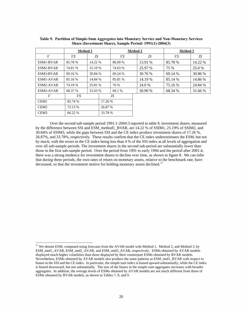
Table 9. Partition of Simple-Sum Aggregates into Monetary Service and Non-Monetary Services Share (Investment Share), Sample Period: 1991(1)-2004(3)
Method 1 Method 2 Method 3 V VS IS VS IS VS ISESM1-BVAR 85.78 % 14.22 % 86.09 % 13.91 % 85.78 % 14.22 % ESM2-BVAR 74.81 % 25.19 % 74.03 % 25.97 % 75 % 25.0 % ESM3-BVAR 69.16 % 30.84 % 69.24 % 30.76 % 69.14 % 30.86 % ESM1-AVAR 85.16 % 14.84 % 85.81 % 14.19 % 85.14 % 14.86 % ESM2-AVAR 74.19 % 25.81 % 76 % 24.0 % 75.16 % 24.84 % ESM3-AVAR 68.37 % 31.63 % 69.1 % 30.90 % 68.34 % 31.66 % V VS ISCEM1 82.74 % 17.26 % CEM2 73.13 % 26.87 % CEM3 66.22 % 33.78 %
Over the second sub-sample period 1991:1-2004:3 reported in table 9, investment shares, measured by the difference between SSI and ESM_method1_BVAR, are 14.22 % of SSIM1, 25.19% of SSIM2, and 30.84% of SSIM3, while the gaps between SSI and the CE index produce investment shares of 17.26 %, 26.87%, and 33.78%, respectively. These results confirm that the CE index underestimates the ESM, but not by much, with the errors in the CE index being less than 4 % of the SSI index at all levels of aggregation and over all sub-sample periods. The investment shares in the second sub-period are substantially lower than those in the first sub-sample period. Over the period from 1991 to early 1994 and the period after 2001:4, there was a strong tendency for investment shares to decline over time, as shown in figure 8. We can infer that during these periods, the own rates of return on monetary assets, relative to the benchmark rate, have decreased, so that the investment motive for holding monetary assets declined.17
17 We denote ESM, computed using forecasts from the AVAR model with Method 1, Method 2, and Method 3, by ESM_mtd1_AVAR, ESM_mtd2_AVAR, and ESM_mtd3_AVAR, respectively. ESMs obtained by AVAR models displayed much higher volatilities than those displayed by their counterpart ESMs obtained by BVAR models. Nevertheless, ESMs obtained by AVAR models also produce the same patterns as ESM_mtd1_BVAR with respect to biases in the SSI and the CE index. In particular, the simple sum index is biased upward substantially, while the CE index is biased downward, but not substantially. The size of the biases in the simple sum aggregates increases with broader aggregates. In addition, the average levels of ESMs obtained by AVAR models are not much different from those of ESMs obtained by BVAR models, as shown in Tables 7, 8, and 9.
20
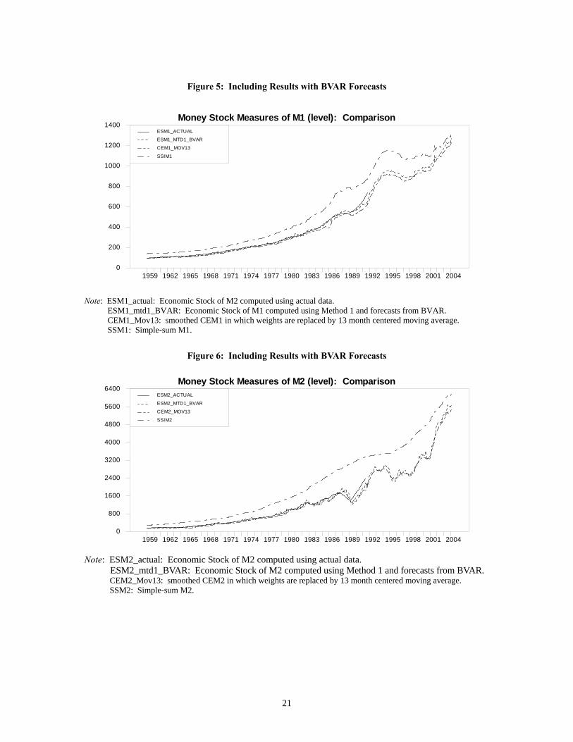
Figure 5: Including Results with BVAR Forecasts
Money Stock Measures of M1 (level): Comparison
1959 1962 1965 1968 1971 1974 1977 1980 1983 1986 1989 1992 1995 1998 2001 20040
200
400
600
800
1000
1200
1400ESM1_ACTUAL
ESM1_MTD1_BVAR
CEM1_MOV13
SSIM1
Note: ESM1_actual: Economic Stock of M2 computed using actual data. ESM1_mtd1_BVAR: Economic Stock of M1 computed using Method 1 and forecasts from BVAR. CEM1_Mov13: smoothed CEM1 in which weights are replaced by 13 month centered moving average. SSM1: Simple-sum M1.
Figure 6: Including Results with BVAR Forecasts
Money Stock Measures of M2 (level): Comparison
1959 1962 1965 1968 1971 1974 1977 1980 1983 1986 1989 1992 1995 1998 2001 20040
800
1600
2400
3200
4000
4800
5600
6400ESM2_ACTUAL
ESM2_MTD1_BVAR
CEM2_MOV13
SSIM2
Note: ESM2_actual: Economic Stock of M2 computed using actual data. ESM2_mtd1_BVAR: Economic Stock of M2 computed using Method 1 and forecasts from BVAR. CEM2_Mov13: smoothed CEM2 in which weights are replaced by 13 month centered moving average. SSM2: Simple-sum M2.
21
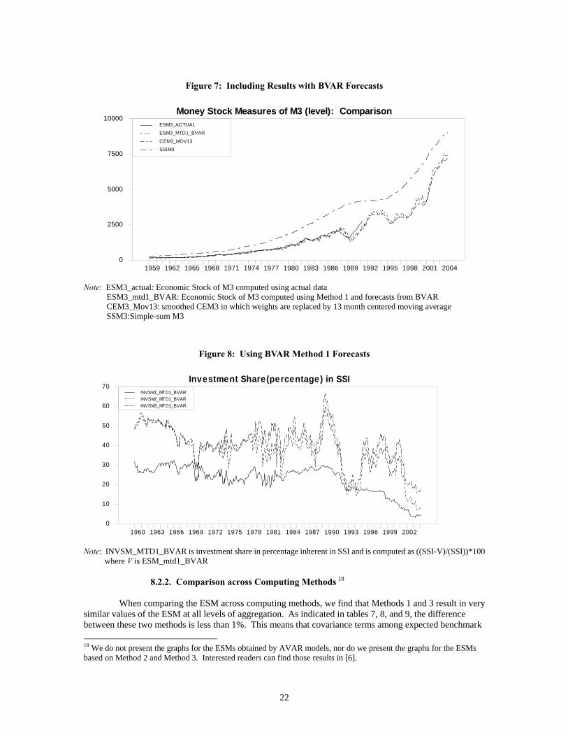
Figure 7: Including Results with BVAR Forecasts
Money Stock Measures of M3 (level): Comparison
1959 1962 1965 1968 1971 1974 1977 1980 1983 1986 1989 1992 1995 1998 2001 20040
2500
5000
7500
10000ESM3_ACTUAL
ESM3_MTD1_BVAR
CEM3_MOV13
SSIM3
Note: ESM3_actual: Economic Stock of M3 computed using actual data ESM3_mtd1_BVAR: Economic Stock of M3 computed using Method 1 and forecasts from BVAR CEM3_Mov13: smoothed CEM3 in which weights are replaced by 13 month centered moving average SSM3:Simple-sum M3
Figure 8: Using BVAR Method 1 Forecasts
Investment Share(percentage) in SSI
1960 1963 1966 1969 1972 1975 1978 1981 1984 1987 1990 1993 1996 1999 20020
10
20
30
40
50
60
70INVSM1_MTD1_BVARINVSM2_MTD1_BVARINVSM3_MTD1_BVAR
Note: INVSM_MTD1_BVAR is investment share in percentage inherent in SSI and is computed as ((SSI-V)/(SSI))*100 where V is ESM_mtd1_BVAR 8.2.2. Comparison across Computing Methods 18
When comparing the ESM across computing methods, we find that Methods 1 and 3 result in very similar values of the ESM at all levels of aggregation. As indicated in tables 7, 8, and 9, the difference between these two methods is less than 1%. This means that covariance terms among expected benchmark 18 We do not present the graphs for the ESMs obtained by AVAR models, nor do we present the graphs for the ESMs based on Method 2 and Method 3. Interested readers can find those results in [6].
22
rates, and covariances between expected benchmark rates and expected monetary-service expenditures, did not seem greatly to affect measurement of the ESM. On the other hand, comparing the ESMs based on Method 1 and Method 2 over the full sample period, we found that monetary service shares estimated by Method 2 were greater than those estimated by Method 1, but the differences between the two methods were less than 3% of the SSI at all levels of aggregation. This divergence between Methods 1 and 2 results from the assumption that the benchmark rate follows a martingale process. Nevertheless, the differences in economic money stock across computing methods seem to be negligibly small, relative to the overall bias in the SSI. Furthermore, regardless of the forecast models from which forecasts are generated, and methods by which ESM is computed, certain patterns are evident. The SSI is biased upward, while the CE index is biased downward, on average, with bias less than 4 % of SSI. 9. Discussion and Conclusion We measure the United States capital stock of money implied by the Divisia monetary-services-flow, in a manner consistent with present-value discounting and time-varying discount rates. Based on Barnett's [4] definition of the economic capital stock of money, we compute the economic stock of money by discounting to present value the expected monetary-services-flow expenditure, with user cost pricing of those flows. The economic stock of money nests the currency equivalent (CE) index as a special case under the assumption of martingale expectations. While the martingale expectations assumption greatly simplifies the present-value discounting, that assumption is very strong and often has motivated hesitancy to use the CE index as a stock measure. Instead of assuming martingale expectations, we use forecasts based on asymmetric vector autoregression (AVAR) and Bayesian vector autoregression (BVAR). For comparison, we compute the ESM using actual realized future data within our sample. We report the size of biases embedded in the SSI and the CE index. Those biases can be attributed to the two indexes’ implicit assumptions. The ESM computed using BVAR forecasts implies that the simple sum index greatly exaggerates money stock through inclusion of substantial non-monetary shares. Over the period 1960:2 to 2004:3, those non-monetary shares comprised 22.76% of the stock at the M1 level, 37.11% at the M2 level, and 41.26% at the M3 level of aggregation. The CE index almost always underestimated the economic stock of money, but the size of the bias in the CE index was less than 4% of the SSI index’s bias at all levels of aggregation. Although the assumption of martingale expectations may be unappealing, the resulting bias of the CE index is very small compared with the bias of the SSI index. A particularly noteworthy conclusion of this research was the robustness of our results across forecasting models. Prior concerns about the use of Barnett’s economic capital stock of money have centered on the difficulties of discounting expected future flows and on the possible need to use sophisticated approaches of forecasting to acquire good results. We find that robustness to the forecasting method is not only high, but is so high that even the simple martingale expectations method implicit in the easily computed CE index may be adequate for most purposes. This conclusion is particularly clear, when the capital stock of money, computed with various models of expectations formation, is compared with the simple sum index. In particular, the variation in capital stock indexes with different expectations formation models is small relative to the gap between any of their paths and that of the simple sum index. Since the difference between the simple sum monetary aggregates and the discounted economic capital stock of money is large, accurate measurement of the theoretical capital stock could have important implications for understanding the wealth effects and transmission mechanism of monetary policy. To do better than the CE index in measuring the growth rate of the monetary-asset capital stock, one can use our BVAR or AVAR model. They both outperformed the “naive” martingale forecast model implicit in the CE index. But data series that depend on forecasted variables are not likely to be preferred by governmental agencies, and we find the gains from forecasting to be small. Although based upon “naive” forecasting, the CE is not atheoretical, unlike the atheoretical simple-sum accounting index. In addition the CE index can easily be computed using data at a single point in time, with moving average smoothing of that otherwise highly volatile index. In conclusion, the CE index can be used to measure the stock of money with reasonable accuracy, while the official simple-sum aggregate is an inappropriate measure of money stock or monetary-services flow. While the use of BVAR or AVAR forecasting can produce small gains for research purposes, we believe
23
that the moving-average-smoothed CE index may be adequate for most policy purposes requiring a money stock variable. We believe using an appropriate measure of money stock can produce advances in understanding the wealth effects of policy. The prior hesitancy to use the theoretical economic capital-stock of money formula no longer is justified, since our finding of robustness of that formula to expectations formation removes the reason for that concern, when judged relative to the simple sum index. Further improvements could be acquired from an adjustment to the CE index to remove the small systematic bias that we identify in that index. Introduction of risk aversion also merits research, using the approach in Barnett and Wu (2005) to risk-adjust the flow that is discounted in the ESM. Having established merits of the asset-pricing capital-stock approach to money measurement, we leave such possible refinements to future research. But it is important to recognize that the large gain in moving from the simple-sum index to the ESM, computed with any forecasting procedure, far exceeds the gains from bias correction, risk adjustment, or choice among forecasting procedures.
------------------------------------------------------------------------------------------------------------------------------
APPENDIX
Table A1. Out-of-Sample Forecast Performance Statistics: UVAR and AVAR
UVAR-M2 AVAR-M2 1U 2U 1U 2U Evaluation Period
2( )mTE BENCH 2( )mTE BENCH 1991:1-2004:3 0.721 0.763 0.716 0.738 1991:1-1995:12 0.771 0.838 0.7567 0.810 1996:1-2001:12 0.737 0.762 0.733 0.711 2002:1-2004:3 0.75 0.768 0.749 0.776
UVAR-M3 AVAR-M3 1U 2U 1U 2U Evaluation Period
3( )mTE BENCH 3( )mTE BENCH 1991:1-2004:3 0.722 0.765 0.72 0.738 1991:1-1995:12 0.777 0.837 0.766 0.81 1996:1-2001:12 0.749 0.763 0.75 0.711 2002:1-2004:3 0.76 0.78 0.753 0.777
UVAR-M1 AVAR-M1 1U 2U 1U 2U Evaluation Period
1( )mTE BENCH 1( )mTE BENCH 1991:1-2004:3 0.747 0.767 0.730 0.737 1991:1-1995:12 0.797 0.839 0.773 0.801 1996:1-2001:12 0.776 0.769 0.741 0.715 2002:1-2004:3 0.724 0.769 0.758 0.791
24
References 1. Barnett, W.A.: The user cost of money, Economics Letter 1, 145-149 (1978). Reprinted in: Barnett, W. A., Serletis, A. (eds.) The theory of monetary aggregation. Amsterdam: North Holland 2000 2. Barnett, W.A.: Economic monetary aggregates: an application of aggregation and index number theory, Journal of Econometrics 14, 11-48 (1980). Reprinted in: Barnett, W. A., Serletis, A. (eds.) The theory of monetary aggregation. Amsterdam: North Holland 2000 3. Barnett, W. A.: Understanding the new Divisia monetary aggregate, Review of Public Data Use 11, 349-355 (1983). Reprinted in: Barnett, W. A., Serletis, A. (eds.) The theory of monetary aggregation. Amsterdam: North Holland 2000 4. Barnett, W. A.: A reply to Julio J. Rotemberg. In: Belongia, M.T. (ed) Monetary policy on the 75th anniversary of the federal reserve system. Boston: Kluwer Academic, 232-244 (1991). Reprinted in: Barnett, W. A., Serletis, A. (eds.) The theory of monetary aggregation. Amsterdam: North Holland 2000 5. Barnett, W.A.: Exact aggregation under risk. In: Barnett, W. A., Salles, M., Moulin, H., Schofield, N. (eds.) Social choice, welfare and ethics. Cambridge: Cambridge University Press 1995. Reprinted in: Barnett, W. A., Serletis, A. (eds.) The theory of monetary aggregation. Amsterdam: North Holland 2000 6. Barnett, W. A., Chae, U., Keating, J.: Forecast design in monetary capital stock measurement. In: Berglund, P. G., Ussher, L. J. (eds.) Critical perspectives on recent developments in macroeconomics. London and N. Y.: Routledge 2006 7. Barnett, W. A., Liu, Y., Jensen, M.: The CAPM risk adjustment for exact aggregation over financial assets, Macroeconomic Dynamics 1, 485-512 (1997). Reprinted in: Barnett, W. A., Serletis, A. (eds.) The theory of monetary aggregation. Amsterdam: North Holland, Amsterdam 2000 8. Barnett, W. A., Wu, S.: On the user costs of risky monetary assets, Annals of Finance 1, 35-50 (2005) 9. Blanchard, O. J., Fischer, S.: Lectures on macroeconomics. Cambridge: MIT Press 1989 10. Diewert, W. E.: Exact and superlative index numbers, Journal of Econometrics 4, 115-145 (1976) 11. Doan, T., Litterman, R. B., Sims, C.A.: Forecasting and conditional projection using realistic prior distributions, Econometric Reviews 3, 1-144 (1984) 12. Hoover, K. D., Perez, S. J.: Post hoc ergo propter once more: an evaluation of “does monetary policy matter? in the spirit of James Tobin, Journal of Monetary Economics 34, 89-99 (1994) 13. Keating, J. W.: Asymmetric vector autoregressions, Proceedings of the Business and Economic Statistics Section of the American Statistical Association 88, 68-73 (1993) 14. Keating, J. W.: Macroeconomic modeling with asymmetric vector autoregressions, Journal of Macroeconomics 22, 1-28 (2000) 15. Litterman, R. B.: Forecasting with Bayesian vector autoregression - five years of experience, Journal of Business and Economic Statistics 4, 25-38 ( 1986) 16. Rotemberg, J. J.:.Commentary: monetary aggregates and their uses. In: Belongia, M.T. (ed) Monetary policy on the 75th anniversary of the federal reserve system. Boston: Kluwer Academic, 232-244 (1991). 17. Rotemberg, J. J., Driscoll, J. C., Poterba, J. M.: Money, output and prices: evidence from a new monetary aggregate, Journal of Business and Economic Statistics 13, 67-83 (1995) 18. Schunk, D. L.: The relative forecasting performance of the Divisia and simple sum monetary aggregates, Journal of Money, Credit and Banking 33, 272-283 (2001) 19. Sims, C. A.: Macroeconomics and reality, Econometrica 48, 1-48 (1980)
25