1

Money and Banking

Notes for the Money and Banking students, Course BSB 6301, in Bahrain Polytechnic

Section Title Page

1 Bahrain Economy and Financial System 2

2 Money and the Financial System 14

3 Commodity Markets 42

4 Macro-Economics 59

5 The British Financial System 75

6 The US Financial System 88

7 The Eurozone and its currency 108

8 Asset Valuation 126

9 Bills, Bonds and Interests Rates 139

10 International Finance 150

2

Bahrain Economy and Financial System

Introduction

This section covers Bahrain’s population and employment, resources, economy, government

budget, currency and exchange rate, financial institutions, “Vision 2030” and the

International Competitiveness Survey.

Bahrain covers an area of 750 square kilometers but has a sea area of 7,500 square

kilometers. Bahrain only has a very small amount of agricultural land and is therefore highly

dependent on food imports. Bahrain has a rapidly depleting oil and gas resource which

underpinned the economy in the past. Bahrain therefore urgently requires economic

diversification. A very good source of information on all countries including Bahrain is CIA

Bahrain.

Bahrain Population and Employment

Table 1

The Population of Bahrain in 2011 was:

Bahrainis 584,688

Non-Bahrainis 610,322

Total 1,195,020

Table 2, below, shows the rapid growth in the population of the country since the first

census was taken in 1941.

Table 2

Year Bahrainis Non-Bahrainis Total

1941 74k 15k 89k

1971 178k 38k 216k

1981 238k 112k 351k

1991 323k 185k 508k

2001 406k 245k 650k

2011 585k 610k 1,195k

Source for Tables 1 and 2, Central Informatics organization

The Bahraini part of the population is growing steadily at about 2.0% pa. In 2013 there were

15k births and only 2k deaths among the Bahraini section of the population.

The Non-Bahraini part has grown very rapidly but the rate of growth is very unstable, eg -

the number fell by over 7% between 2010 and 2011, and varies with the state of the

economy.

3

Bahrain is highly dependent on a Non-Bahraini workforce as they make up 77% of the

workers in the Country. The Table below shows the workforce in different sectors.

Table 3

Employment in Sectors Total Bahrainis Non-Bahrainis

Manufacturing 81k 15k 65k

Construction 131k 11k 120k

Trade 127k 24k 103k

Finance 14k 9k 5k

Government 58k 53k 5k

Domestic 95k 0k 95k

Other 142k 36k 107k

Total 648k 148k 500k

Source, Bahrain Economic Development Board

The Employment Participation Rate in Bahrain is low by international standards. The

standard method of measuring Employment Participation Rates is to calculate the

percentage of the population aged between 24 and 65 who are working. The table below

gives Employment Participation rates for Bahrain and the 27 countries of the European

Union. The Participation Rates for Bahraini Females is very low by international standards.

Table 4

Bahrain EU 27

Male 82% 74%

Female 40% 62%

Total 61% 68%

Sources, Bahrain CIO and Eurostat

The Bahrain Population and workforce can be represented as a pyramid. This diagram is

copied for the 2013 Annual Report of the Bahrain Economic Development Board. The shape

of the population pyramid reflects the rapid population growth and youn age structure of

the population.

4

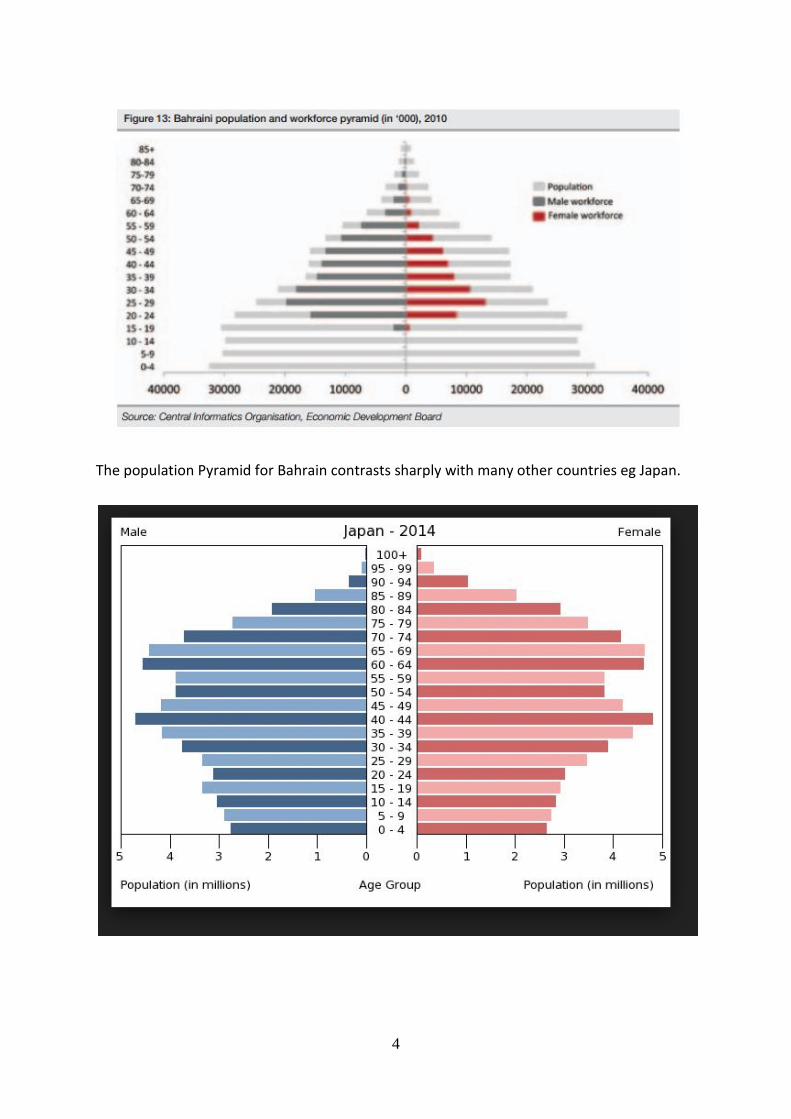
The population Pyramid for Bahrain contrasts sharply with many other countries eg Japan.

5

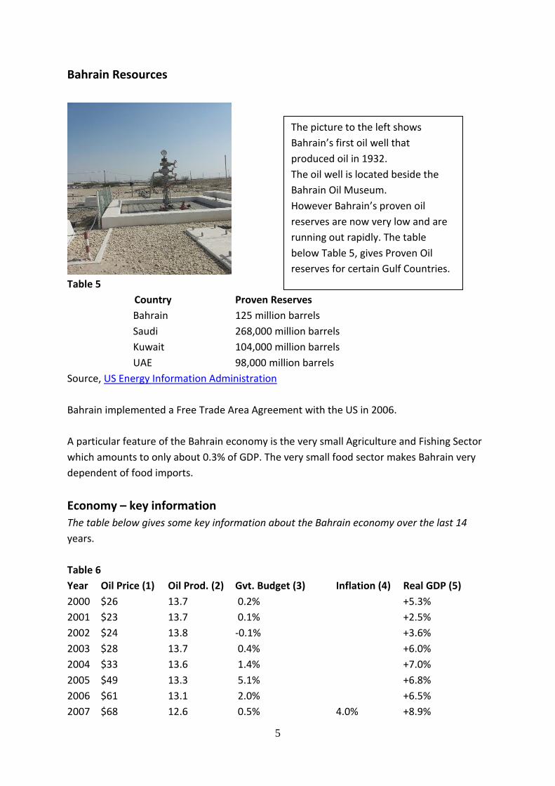
Bahrain Resources

Table 5

Country Proven Reserves

Bahrain 125 million barrels

Saudi 268,000 million barrels

Kuwait 104,000 million barrels

UAE 98,000 million barrels

Source, US Energy Information Administration

Bahrain implemented a Free Trade Area Agreement with the US in 2006.

A particular feature of the Bahrain economy is the very small Agriculture and Fishing Sector

which amounts to only about 0.3% of GDP. The very small food sector makes Bahrain very

dependent of food imports.

Economy – key information

The table below gives some key information about the Bahrain economy over the last 14

years.

Table 6

Year Oil Price (1) Oil Prod. (2) Gvt. Budget (3) Inflation (4) Real GDP (5)

2000 $26 13.7 0.2% +5.3%

2001 $23 13.7 0.1% +2.5%

2002 $24 13.8 -0.1% +3.6%

2003 $28 13.7 0.4% +6.0%

2004 $33 13.6 1.4% +7.0%

2005 $49 13.3 5.1% +6.8%

2006 $61 13.1 2.0% +6.5%

2007 $68 12.6 0.5% 4.0% +8.9%

The picture to the left shows

Bahrain’s first oil well that

produced oil in 1932.

The oil well is located beside the

Bahrain Oil Museum.

However Bahrain’s proven oil

reserves are now very low and are

running out rapidly. The table

below Table 5, gives Proven Oil

reserves for certain Gulf Countries.

6

2008 $94 12.0 3.9% 0.5%* +3.1%

2009 $62 11.8 -8.4% 1.6% +2.7%

2010 $78 11.1 -8.0% 1.0% +4.4%

2011 $106 15.5 -3.0% 0.2% +1.9%

2012 $110 16.6 -2.0% 2.6% +3.4%

2013 $105 -5.3% 4.0% +5.3%

2014 $96 +4.5%

(1) $ per barrel. Source, World Bank, Dubai Price Series

(2) Crude Oil produced in Bahrain in millions of barrels pa. Source, BEDB, Economic

Development Board

(3) Budget Surplus/Deficit as % of GDP. Source, Ministry of Finance,

https://www.mof.gov.bh/

(4) Consumer price Index, Source, Central Informatics Organization, * November 2008

(5) GDP Growth adjusted for inflation, Source, BEDB

Government Budget

The Bahrain Government Budgets for 2013 and 2014 are as follows:

Table 7

Revenue in millions of BD 2013(O) 2014(F) 2014(O) 2015(F)

Oil and Gas Revenue 2,600 2,404 2,662 1,824

Taxation and Fees 224 199 203

Gvt. Goods and Services 53 54 54

Investments and Gvt. Property 18 76 82

Grants 0 38 28

Sale of Capital Assets 0 0 1

Fines, Penalties and Miscellaneous 49 22 59

Total Revenue 2,944 2,793 3,089 2097

Recurrent Expenditure

Manpower 1,300 1,393 1,379

Services 211 193 223

Consumables 131 144 148

Assets 31 34 36

Maintenance 67 68 69

Transfers 695 800 729

Grants and Loan Interest 442 520 511

Total Recurrent Expenditure 2,877 3,153 3,096 3,136

Projects 477 826 448 435

Total Expenditure 3,354 3,978 3,544 3,570

Surplus (Deficit) in Budget (410) (1185) (455) (1,474)

7

Notes, (O) = Outturn, (F) = Forecast

Sources Ministry of Finance, Consolidated Final Accounts

Ministry of Finance, Projections for 2015 and 2016

The dependence of Bahrain on Oil and Gas Revenue, which are both subject to commodity

price fluctuations, makes budgeting very difficult.

The Next table shows the Overall Budget Outturn for the Bahrain Government for the last

14 years:

Table 8

Year Revenue Expenditure Balance

2005 1,671 1,289 382

2006 1,840 1,558 281

2007 2,037 1,818 219

2008 2,678 2,173 547

2009 1,708 2,154 -446

1020 2,176 2,635 -460

2011 2,821 2853 -31

2012 3,034 3,261 -226

2013 2,944 3,354 -410

2014 3,098 3,544 -455

Sources, Ministry of Finance,

The Budget Deficits of recent years are leading to an increase in Bahrain’s National Debt.

The Table below gives the Bahrain’s Public Debts Instruments as a % of GDP for some recent

years.

Table 9

Year Public Debt Instruments as % of GDP

2009 18.3%

2010 29.0%

2011 29.0%

2012 33.9%

2014 41.4%

Source CBB, Economic Indicators

Bahrain Government Bonds have a BBB rating with Standard and Poor and the rates of

interest on Bahrain Government Bills and Bonds are given below on page 10 below.

8

Currency and Exchange Rate

The major currency in use in Bahrain up to 1959 was the Indian Rupee issued by Reserve

Bank of India. The Rupee was pegged to the £ Sterling at 13.33 = £. Rupees circulating in

the Gulf were used to circumvent Indian restrictions on the purchase of gold. In 1959 the

Reserve Bank of India issued a new “Gulf Rupee” which had the same value as the “Indian

Rupee” but which had restriction on its use for purchasing gold.

The Gulf Rupee was the dominant currency in Bahrain from 1959 to 1965. In 1965 Bahrain

set up the Bahrain Currency Board and introduced the Bahrain Dinar (BD). The value of the

BD was set at 1.86621 grams of gold and 10 Gulf Rupees. (The BD has strengthened relative

to the Rupee and is now, December 2014, worth 164 Rupees) The notes were printed by De

La Rue in London. The BD became the Legal Tender in Bahrain and the Gulf Rupees were

exchanged for BDs.

After independence in 1971 Bahrain set up the Bahrain Monetary Agency to act as a Central

Bank for Bahrain. The Bahrain currency was rocked by counterfeiting of BD 20 notes in 1998

but this was overcome by printing a new set of BD 20 notes.

In 2006 the Central Bank of Bahrain (CBB) was set up and it took over the duties of the

Bahrain Monetary Agency. The CBB is responsible for Monetary Policy and Bank Regulation.

http://www.cbb.gov.bh/

Bahrain has a long history of pursuing a fixed exchange rate policy. The Economist Magazine

reported on August 1st 1964 that one of the reasons that Bahrain was going to introduce its

own currency was “to avoid being pulled into a forced devaluation by India”. The Dinar was

pegged to the $ in 1980. In 2001, the fixed exchange rate with the USD was made official.

Bahrain is committed to an exchange rate peg at BHD 0.376 per US Dollar, corresponding to

approximately BHD 1 = USD 2.65957.

The exchange rate peg aims at protecting the currency’s external value while ensuring

internal price stability. Within this framework, the Central Bank has flexibility to alter

domestic monetary conditions by changing policy interest rates, introducing prudential

guidelines on bank lending and adjusting reserve requirements to achieve the required

balance between price stability and growth.

Since Bahrain is a small and open economy with foreign trade accounting for more than

110% of nominal GDP, the exchange rate represents a logical anchor for monetary policy. It

reduces transaction costs and exchange rate uncertainty, and thereby stimulates trade.

Given the role of the US Dollar as the leading global reserve currency as well as its central

role in international trade and finance, pegging the Bahrain Dinar to the Dollar enhances the

credibility of monetary policy and contributes to financial stability.

9

The Central Bank of Bahrain (CBB) defines its role as “the main authority responsible for

maintaining monetary and financial stability, and having the instruments and operational

independence in pursuing its policy objectives. It is also the single integrated regulator of

Bahrain’s financial industry “.

The CBB utilizes three main monetary policy instruments to influence liquidity conditions in

the banking sector:

Exchange rate facility: CBB offers to buy/sell Bahraini Dinars against the US

Dollar at rates very close to the official exchange rate. CBB provides this

facility to all commercial banks located in the Kingdom of Bahrain.

Standing facilities: A set of lending and deposit facilities designed to influence

overnight liquidity, overnight interest rates and steering the short-term

money market to the key policy rate determined by the CBB. The lending

facilities are Overnight Secured Loans and One week Repo Loans. The rate of

interest on these loans was 2.25% in June 2014. The rate of interest on

deposits was 0.5% in June 2014.

Reserve Requirements: All commercial banks operating in the Kingdom of

Bahrain are required to maintain reserves deposited at the CBB amounting to

5% of the value of non-bank deposits denominated in Bahraini dinars. The

reserves are not remunerated.

The Bahrain Central Bank is responsible for Financial Stability in Bahrain. The central bank

licences and regulates the banks in Bahrain and if any bank gets into trouble the CBB will

intervene to protect depositors or other creditors. In July 2009 Bahrain's central bank took

control of Awal Bank because there was a substantial shortfall in their assets relative to

their liabilities. This decision was appealed in court by persns linked to Awal bank but the

court found that CBB had acted legally

Financial Institutions

Bahrain has a very large financial services industry relative to the size of the economy. In

2012 the country had 405 firms involved in financial services.

Table 10

Category Number of Firms

Conventional Banks 77

Islamic Banks 26

Insurance Companies 152

Investment Firms 49

Specialized Financial Firms 79

Capital Markets Firms 22

Total 405

10

Source CIO

The Money Supply in Bahrain at the end of April 2014 was as follows:

Table 11

Category BD in Millions

Currency outside the banking system 486

Private Demand Deposits 2,468

M1, Narrow Money Supply 2,953

Term and Savings Deposits 6,650

M2, Medium Money Supply 9,603

Government Deposits 1,821

M3, Broad Money Supply 11,425

Source CBB, Page 3

The table below gives some aggregated information about the Assets of the Bahrain banking

System:

Table 12

Category BD billions

Total Assets of Banking System 193

Retail Bank Assets 78

Wholesale Bank Assets 115

Islamic Banks 24

Domestic Assets 50

Source, CBB

The Lending by the Banking System was broken down as follows by Sector for end of 2012.

Table 13

Business Sector Total Lending

Personal 2,368

Government 198

Transport 249

Trading 960

Construction 1,642

Agriculture and Fishing 12

Mining and Quarrying 9

Manufacturing 538

Others 874

Total 6,849

Source CBB, Page 9

11

An interesting feature of Bahrain bank lending was the rapid growth in Bank Lending to

Construction between the end of 2005 and the end of 2008. During this period the total

lending by Bahrain banks to the construction Industry increased from BD302 million to BD

1540 million. This massive growth in bank lending followed the pattern in many parts of the

world including the US where bank lending fuelled a property bubble.

The Interest rates on various Financial Assets was as follows for April 2014:

Table 14

Financial Asset Interest Rate

Personal Loans 6.24%

Business Loans 4.73%

Interest on Deposits 1.05%

Money market rates, 3 Months 0.24%

Money market rates, 6 Months 0.34%

Treasury Bills, 3 Months 0.87%

Treasury Bills, 6 Months 1.08%

Treasury Bills, 12 Months 1.25%

Source, CBB

The CBB issues Government Bonds on behalf of the Government. An example is as follows,

GDEV. BND 19 which was issued on 08/11/2012 and will mature on 08/11/2019. This was

issued in BD1,000 units and has an interest rate of 4.3%. The average rate of interest on

Bahrain Government Bonds was 2.62% in April 2014

The rates of interest on the Bahrain Money market over the last 9 years are shown in the

next diagram which is taken from the BEDB 2013 Annual Report.

12

Vision 2030

Vision 2030 is a comprehensive long-term economic and social vision for the development

of Bahrain. Vision 2030 was adopted in 2008 after wide consultation. Bahrain Vision 2030 is

a vision for Bahrain as it addresses the issues linked to a decline in oil revenues and a rapidly

growing population. Oil revenues played a vital role in the economy of the country for the

last 80 years. The population of Bahrain is growing rapidly with the population growing by

over 13 times between 1941 and 2011.

The following extracts from the document highlight some of the challenges facing Bahrain:

“We aspire to shift from an economy built on oil wealth to a productive, globally

competitive economy, shaped by the government and driven by a pioneering private sector

– an economy that raises a broad middle class of Bahrainis who enjoy good living standards

through increased productivity and high wage jobs.”

“Our society and government will embrace the principles of sustainability and fairness to

ensure that every Bahraini has the means to live a secure and fulfilling life and reach their

full potential”.

“Bahrain is facing a shortage of both quality employment and appropriate skills.”

“4,000 Bahrainis a year are entering the job market with at least a college degree. The

private sector is creating on average only 1,100 jobs per annum with a monthly salary of at

least BHD 500 for Bahrainis and about 2,700 for non-Bahrainis.”

“Bahrainis are not the preferred choice for employers in the private sector since the

education system does not provide the young people with the skills and knowledge needed

to succeed in our labour market.”

“For many years Bahrain has been able to address these issues by redistributing oil revenues

and offering citizens jobs in the public sector. This has left us with an oversized public sector

– a situation that will be unsustainable in the future considering the gradual decline of oil

revenues.”

“The sustainability of government finances is strengthened by reducing dependence on oil

revenues to fund current expenditure”

“The most sustainable way of resolving the imbalance and raising the quality of employment

is a transformation to an economy driven by a thriving private sector – where productive

enterprises, engaged in high value added activities offer attractive career opportunities to

suitably skilled Bahrainis.”

13

“On a Global scale, Bahraini innovation is currently negligible.”

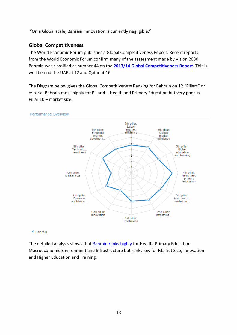
Global Competitiveness

The World Economic Forum publishes a Global Competitiveness Report. Recent reports

from the World Economic Forum confirm many of the assessment made by Vision 2030.

Bahrain was classified as number 44 on the 2013/14 Global Competitiveness Report. This is

well behind the UAE at 12 and Qatar at 16.

The Diagram below gives the Global Competitiveness Ranking for Bahrain on 12 “Pillars” or

criteria. Bahrain ranks highly for Pillar 4 – Health and Primary Education but very poor in

Pillar 10 – market size.

The detailed analysis shows that Bahrain ranks highly for Health, Primary Education,

Macroeconomic Environment and Infrastructure but ranks low for Market Size, Innovation

and Higher Education and Training.

14

Money and the Financial System

Introduction

Money and the financial system play a complex and central role in the functioning of the

modern economy. This note on money and the financial system will cover the definition of

money, the role of money, how money affects the real economy, the evolution of

commercial banks, the Bank of England, bank licensing and regulation, money creation by

banks, the 2007/08 financial crisis, the Gold Standard, British Inflation during the 20th

century, inflationary spirals and hyperinflation, deflation, Fisher’s Equation, the role of a

central bank, financial stability, Systemically Important Banks, Monetary Policy,

“Unconventional Monetary Policy” and inflation targets. This section ends with a Glossary of

Banking Terminology from the Central Bank of Bahrain Rulebook.

Definition of Money

Money is a highly complex social convention for the recording of debts and obligations

arising out of exchange transactions. A social convention gives meaning to something that is

accepted by most members of a community and therefore influences the actions of persons

within that community. Language is a social convention in that members of the language

community accept the meaning of words and use these words in accordance with rules that

give these words meaning. Money is a social convention in that members of that economic

community accept it as a form of payment for goods and services on the understanding that

it can be used to buy the equivalent value of goods and services at some point in the future.

Language evolved in human communities because communication was vital for human

survival. Money evolved as a social convention because it allows exchange to operate much

more efficiently especially in large and complex communities. Efficient exchange was

needed to allow communities take advantage of the benefits of specialization in production

Money is enormously difficult to define. The Collins Reference Dictionary of Economics, for

example, defines money as “An asset that is generally acceptable as a medium of

exchange”. In a historical sense this definition is correct in that money originated with the

use of real assets such as gold in exchange. Modern forms of money including coins, paper

money and bank deposits are not “real assets”. These forms of money are claims on a share

of the real resources (assets, goods and services) that are traded within a community. The

claim is guaranteed by the organization, or the community which the organization

represents, issuing the money. So a better definition of money is “A claim to a share of the

real resources that are traded in a community that is issued and guaranteed by an

organization which has the credibility to have its guarantees accepted”. The person who has

a Bahrain Dinar has a note which allows him/her to claim one BD’s worth of resources that

15

are traded in Bahrain and the Central Bank of Bahrain has the credibility to have its

guarantee accepted.

Money is totally different when seen from the perspective of any individual or

group/organisation in a community or the perspective of that community as a whole.

Economics looks at the functioning of the economy from the perspective of the overall

community so economics usually looks at money from that perspective.

Business looks at money from the perspective of an individual or group/organisation within

the community. Money, looked on from this perspective, is an asset and the more money

the individual or group/organization has then the richer they are. From the perspective of

the overall community, however, money is not an asset and an increase in the amount of

money in circulation will not make the community richer. From the point of view of the

overall community money is merely a way of keeping the economy functioning. Adam

Smith, the Scottish Economist, described money as a “great wheel of circulation” in his book

The Wealth of Nations , p 235, which was published in 1776 (Pennsylvania University

eCopy).

The definition of money by central banks as M1, M2 or M3 depends on how easily the

money can be spent. M1, the simplest definition of money, involves money in a form that

can be spent immediately. MI involves cash and demand deposits held by the public

(individuals and all non-bank organisations).

Role of Money

In any well-functioning economy money fulfills the following roles, Medium of Exchange

Measure of Value

Store of Value

By medium of exchange is meant that goods and services are not exchanged directly for

each other as in barter but that money is used as an intermediary. In a modern economy the

exchange value or price of goods and services is measured in money. Wealth can be saved in

money whether it is cash or bank deposits.

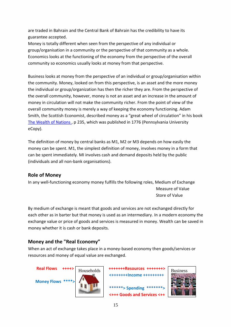
Money and the "Real Economy”

When an act of exchange takes place in a money-based economy then goods/services or

resources and money of equal value are exchanged.

Real Flows ++++> +++++++Resources +++++++>

<+++++++Income +++++++++

Money Flows ****>

******> Spending *******>

<+++ Goods and Services <++

Households

Business

16

When looking at an economy you can focus on the money flows (****) or focus on the

goods/services and resources (++++) which are being exchanged for the money. If you are

focusing on the goods and services which are being produced and exchanged, instead of on

the money flows, you are said to be dealing with the “Real Economy”.

In the US this distinction is often put as “Wall Street” and “Main Street”. When the financial

system came under stress in 2007/2008, policy makers were concerned to ensure that the

problems of the financial system did not push the economy into a deep recession. This was

described as preventing “Wall Street” from affecting “Main Street”.

The Financial System is so important to the modern economy that the maintenance of an

efficient financial system is a key priority of most governments. This was shown by the

global reaction to the financial crisis of 2008 where there was an orchestrated global

reduction of central bank interest rates and coordinated refinancing of banks in the EU,

Britain, Japan, China and the US.

History of Money

The money systems which we use evolved over many years from the bartering of goods and

services directly for each other.

Barter economy

Use of items of intrinsic value as money

Use of coins made from precious metal

Receipts for gold as Paper Money

Paper Money

Bank Deposits

The simplest exchange system is that of barter where goods and services are exchanged

directly for each other. Barter, however, is a very cumbersome method of exchange. Barter

remained important in parts of Europe into the 19th century. When farmers were selling

their grain in the public markets of Europe they often had to give a 1/32nd part to the owner

of the market.

In traditional societies there was only limited use of money. People exchanged goods and

services among each other within the local community based on well understood rights and

obligations without the use of money. These rights and obligations were based on custom

and law. In Europe the social system known as Feudalism was based on the ordinary people

who were known as Serfs having the right to work land that was allocated to them and to

receive protection from the Lord in exchange for labour, goods and service.

17

Up to the 1950s farmers in the West of Ireland often exchanged “days”. Farmer A would

help farmer B for a number of days and B would end up “owing” A that number of days and

would pay back these days at some future time. Farmers who exchanged days would often

be linked by blood or friendship connections. Occasionally one day owed might be

transferred to a third farmer. If B owed A one day and if A owed C one day then the debts

could be settled by B giving C one day.

The exchange of goods and services without the use of money and the consequent debts

and obligations, can only work on a small scale and at a local level so precious metals were

used in different societies as ways of recording these debts or claims and obligations when

exchanges spread beyond the local level. There are however significant difficulties with

using precious metals to record debts. These difficulties are linked to the weighing of metals

and assessing the purity of metals.

Coins were minted and stamped with a state seal to guarantee their weight and purity. The

first gold coins were minted by Croesus, King of Lydia, (modern-day Turkey), in the period

560 to 546 BC. Minted coins became the accepted money in all countries. The original

English silver penny contained 1/240 of a pound of pure silver and so the English pound

Sterling, being worth 240 pennies, was equivalent to a pound (lb Troy measure) of pure

silver. (The Troy pound is about 37% of a Kilogram).

Bank notes, which were, in effect, receipts for silver or gold, started to circulate at the end

of the 17th century. The first bank notes in Britain were those circulated in London by the

“Goldsmith Bankers”. These were receipts for gold. Bank deposits, whose ownership can be

transferred by cheques or EFT (Electronic Funds Transfer), are now the major form of

money. The Money Supply now consists of cash held by the public and bank deposits. There

are different technical definitions of the Money Supply chiefly depending on whether or not

Time Accounts are included. M1, which is the money supply narrowly defined, just includes

cash held by the public and demand deposits of the private sector.

Central Bank of Bahrain Financial Statistics show that M1 for Bahrain was BD2,943 million in

April 2014. M2 includes cash and all private sector bank deposits. M2 for Bahrain was

BD9,603 million. M3, which is the money supply broadly defined, also includes all bank

deposit, both private and public sector. M3 for Bahrain in April 2014 was BD11,425 million.

Evolution of Commercial Banks

Commercial Banks in Europe gradually evolved from the business of Goldsmiths and

Moneylenders who provided a safe storage facility to merchants and stored their gold and

silver coins.

18

The first modern bank is believed to have been set up in Venice in Italy in 1157. Venice was

then a great trading city and port. The oldest surviving bank in the world is the Monte dei

Paschi di Siena Bank (MPS), of Siena in Italy, which was founded in 1472. MPS made losses

of €7 billion in 2011 and failed the ECB stress testing in 2014. This created a situation where

MPS was required to increase its capital by €2 billion.

Accounting was invented by Italian Bankers and was widely practiced in Italy after 1300.

(The first book on accounting by Luca Pacioli, explaining double entry, was only published in

1494 in Venice).

Italian goldsmiths and moneylenders started to arrive in Britain at the end of the 13th the

century from Florence, Venice and Genoa. Edward II, King of England gave a grant of land in

the City of London to a group of these goldsmiths, money-lenders and bankers from

northern Italy in 1318. They were called Lombards and the street is called Lombard Street.

They brought with them knowledge of banking and accounting (double entry). The Italian

money lenders also brought the notation for English money £sd, or Lira, Soldi and Denarii.

The development of Banking can be shown by looking at the evolution of the balance sheet

of a representative goldsmith/moneylender/banker in London such as Francis Child.

These businessmen, known as “Goldsmith Bankers”, started storing gold for merchants and

other wealthy persons in London. As London developed into a major trading centre the

need for safe storage of wealth grew. These Goldsmith Bankers developed both their money

storage activities, especially around the time of the English Civil Wars from 1642 to 1651,

and their lending activities and their businesses evolved into banks.

Stage 1 Merchant needed a safe place to store their gold. Francis Child stored gold for a

Merchant for a fee.

Assets Liabilities

Gold in Vault 100 oz Gold from Merchants 100 oz

-------- --------

100 oz 100 oz

(FC was making profits made from storing Gold for Merchants)

Stage 2 Francis Child found that he could lend some of the gold that he was being paid to

store.

Gold in Vault 40 oz Gold from Merchants 100 oz

Loans 60 oz

------- -------

100 oz 100 oz

(FC started making large profits from storing gold and lending the gold stored by him)

19

Stage 3 Francis Child could give loans by issuing Gold Receipts to the borrower.

As the scale of their business expanded Goldsmiths needed to keep better records and

started issuing “Warehouse Receipts” to those who deposited gold with them. These

“Warehouse Receipt” started to circulate among the public as payment for goods and

services. About 1680 Francis Child started issuing these “Warehouse Receipts” in standard

denominations. These are regarded as the first true banknotes in the Western World.

Gold in Vault 40 oz Gold from Merchants 100 oz

Loans by Warehouse Receipts 300 oz Receipts for Gold 240 oz

-------- -------

340 oz 340 oz

(FC started making increased profits from a massively expanded level of Lending)

Stage 4 The balance sheet of a modern bank looks as follows

Assets Liabilities

Cash 2% Capital 10%

Deposits with Central Bank 5% Bonds 10%

Bills and Bonds 18% Money Market 10%

Loans and Investments 73% Current Deposits 20%

Premises and Other Assets 2% Savings Deposits 50%

----- -----

100% 100%

(Profit from Lending and Banking Services)

The Bank of England

In 1694 a group of London businessmen offered the government of William of Orange, who

had recently deposed his father-in law as King of England and was involved in a war with

France, a loan of £1.2 million, at an interest rate of 8% per annum. These businessmen also

got a Royal Charter for a bank, with important privileges, to be known as the Bank of

England.

The Bank of England Notes, in the BoE’s own word’s “became a widely accepted currency as

people seldom doubted that the “promise to pay” which referred to gold coin of the realm

would be honored”. The BoE always redeemed their banknotes with gold coins at the rate of

one gold coin for a pound. (The gold coins which the bank used to redeem one Pound held

0.25 ounces of gold)

From its foundation the BoE acted as the government bank in Britain and managed the

national debt. The bank became the dominant bank in England and Wales. The banks notes

were made legal tender in 1833. The BoE, as the government’s bank, was used by the British

government to manage financial crises and so evolved into what is now called a Central

20

Bank. A Central Bank is a bank that manages the financial system of a country. The BoE was

a private bank from 1694 until it was nationalized in 1946.

Bank Types

There are now a wide variety of bank types or bank categories. These types or categories

vary from country to country so it is impossible to classify banks internationally other than

by the banking services they provide.

The simplest form of banking is deposit taking, personal lending and money transfer. Most

small banks provide these services and these banks are often referred to as “Retail Banks”.

Some banks specialize in providing banking services to business and these are often referred

to as “Commercial Banks”. Some banks, such as Coutts in London, specialize in providing

banking services to high net-worth individuals and these are referred to as “Private Banks”.

Banks, such as Goldman Sachs, that provide a range of advisory and funding services, such

as IPOs and Bond Sales, to large businesses are referred to as “Investment banks”. Goldman

Sachs has been involved in IPOs since they handled the launch of Sears Roebuck on the NYSE

in 1906. Investment Banks are also usually involved in proprietary trading and investment.

Up until 2008 US Investment banks did not hold banking licenses. Banking licenses in the US

restricted banks from engaging in high risk and high profit activities such as proprietary

trading and investment so the investment banks chose to operate without a banking license

to avoid regulation as banks. This however meant that they could not accept deposits or

access emergency funding from the Federal Reserve Bank. During the financial crisis this

form of unregulated US banking disappeared.

Banks in Britain and Europe were much less restricted, by banking legislation, in their

activities so most large British banks such as Barclays and Deutsche Bank provide a full

range of banking services including Retail, Commercial, Private and Investment Banking.

Barclays website says that “Our banking services cover everything from credit cards to

corporate banking, across the globe”.

In Bahrain there are 4 categories of banks. These are Conventional Banks, divided between

Retail and Wholesale, and Islamic Banks, divided into Retail and Wholesale. Conventional

Retail Banks provide the full range of banking services required by ordinary customers such

as deposit accounts, loans, credit card and foreign exchange. The Wholesale banks are

restricted by the scale of deposits as the minimum deposit in a wholesale bank is BD 7

million.

Islamic banks provide a variety of products, including Murabaha, Ijara, Mudaraba,

Musharaka, Al Salam and Istitsna'a, restricted and unrestricted investment accounts,

syndications and other structures used in conventional finance, which have been

21

appropriately modified to comply with Shari’a principles. An example of this is BisB which

provides Retail and Commercial Banking Services in Bahrain.

The CBB has a Register of Banks .There were 78 banks in Bahrain holding “Conventional

Licenses” in May 2015. These involve 22 Conventional Retail Banks and 56 Conventional

Wholesale banks. There were 24 banks in Bahrain holding “Islamic Licenses” in May 2015.

These involve 6 Islamic Retail and 18 Islamic Wholesale Banks.

Bank Licensing and Regulation

Banks are so important in the functioning of a modern economy that they are subject to

much stricter licensing and regulation than ordinary businesses. The systems for Bank

licensing vary from country to country and these systems evolve in response to political and

financial events.

In the US banks can apply for either State Banking Licenses or National Banking Licenses.

Each state has its own Licensing Authority. Holders of state banking licenses can only

operate in the state where they hold a license. In New York the state banks are licensed by

the Department of Financial Services of the State of New York. Banks that are allowed to

operate all over the US are called National Banks and are licensed by the Office of the

Controller of the Currency (Agency within the US Treasury set up in 1863 by President

Lincoln). Federal Savings Banks are licensed by the Office of Thrift Supervision (Agency

within the US Treasury)

In the UK bank licensing in now the responsibility of the Financial Conduct Authority but was

previously the responsibility of the Financial Services Authority . The financial crisis in Britain

in 2008 led to the splitting up of the Financial Services Authority and is role was divided

between the Financial Conduct Authority and the Prudential Regulation Authority , which is

an agency within the Bank of England.

In Bahrain bank licensing is the responsibility of the Central Bank of Bahrain . No person or

company can carry on banking activities in Bahrain without holding a banking license from

the CBB.

A summary of the bank licensing process in Bahrain can be found in the CBB Guide to

Licensing. Complete details of the CBB licensing process and requirements are prescribed in

the CBB Rulebook. Each Volume of the Rulebook contains a Module setting out the CBB's

licensing requirements, with respect to the sector covered by the Volume in question,

including a full description of the relevant Regulated Services. Volume 1 covers

“Conventional Banking and Volume 2 covers Islamic Banking.

Bank Regulation regimes vary significantly from country to country with major differences

between regulation in the US, Britain and Bahrain.

22

US banking regulation is highly complex with banks being subject to regulation by multiple

agencies. The Federal Reserve Bank , the Federal Deposit Insurance Commission , the Office

of the Controller of the Currency , Office of Thrift Supervision and the state bank regulator

are all involved in aspects of bank regulation.

All banks that are members of the Federal Reserve System are regulated by the Federal

Reserve. All banks that accept deposits must be covered by deposit insurance and are

subject to regulation by the Federal Deposit Insurance Corporation. State banks that are not

members of the Federal Reserve System are regulated by the Office of the Controller of the

Currency. Federal Savings banks are regulated by the Office of Thrift Supervision.

In Britain banks are regulated by the Financial Conduct Authority and by the Prudential

Regulation Authority.

Bahrain has a single regulator, the Central Bank of Bahrain. The Central Bank of Bahrain

(CBB), in its capacity as the regulatory and supervisory authority for all financial institutions

in Bahrain, issues regulatory instruments that licensees and other specified persons are

legally obliged to comply with. These regulatory instruments are contained in the CBB

Rulebook. The Regulated Banking Services are:

(a) Deposit-taking (b) Providing Credit (c) Accepting Sharia money placements/deposits (d) Managing Sharia profit/loss sharing investment accounts (e) Offering Sharia Financing Contracts (f) Dealing in financial instruments as principal (g) Dealing in financial instruments as agent (h) Managing financial instruments (i) Safeguarding financial instruments (j) Operating a Collective Investment Undertaking (k) Arranging deals in financial instruments (l) Advising on financial instruments (m) Providing money exchange/remittance services; or (n) Issuing/administering means of payment

Volume 1 covers Conventional Bank Licensees. It contains prudential requirements (such as

rules on minimum capital and risk management). Collectively, these requirements are aimed

at ensuring the safety and soundness of CBB-licensed conventional banks and providing an

appropriate level of protection to the clients of such banks

Volume 2 covers Islamic Bank Licensees. It contains prudential requirements (such as rules

on minimum capital and risk management). Collectively, these requirements are aimed at

ensuring the safety and soundness of CBB-licensed Islamic banks and providing an

appropriate level of protection to the clients of such banks

23

The website version of the Rulebook acts at all times as the definitive version of the

Rulebook.

The CBB Rulebook has a Glossary of Financial terms which may be useful. Some of these

financial terms are explained at the end of this section.

Money Creation by Banks

Bank lending is closely linked to money creation. Bank loans are not counted as money but

bank deposits are included in the money supply. When a person gets a loan from a bank

what normally happens is that the bank opens a loan account and transfers the amount of

the loan from the loan account into the person’s current account. The amount in the current

account is money since it is available for spending. When the borrower spends the money,

for example in the purchase of a house, ownership of the deposits is transferred within the

banking system.

This short video from the Bank of England shows how Money is created when a loan is given

by a bank. It is traditional to see the giving of the loan as the creation of money and the

bank as the creator. However when a loan is given there are two parties involved. The

borrower commits himself/herself to repay the bank so looked at from this perspective the

borrower is involved in creating money by committing herself to repay the bank. The money

is therefore created by the bank risking the loan and the borrower committing her future to

the deal.

Confidence is crucial in bank lending. The person borrowing must be confident that s/he can

repay out of future cash flow and the bank must be confident that it will get its money back.

When a loan is repaid to a bank what normally happens is that money is taken from deposits

to repay the loan. This reduces deposits and therefore reduces the money supply. So the

change in the total amount of lending by banks, how new loans compare with the

repayment of existing loans, is what affects the money supply.

In the examples above the banks took a certain amount of cash and created a much larger

amount of money based on this small cash holding. The power of a single bank in any

country to create money is limited. When any bank gives a loan it will almost certainly

create a deposit at the same time but once the deposit is spent the money will migrate to

another bank so its ability to create deposits is limited. However if all banks are increasing

their lending then the money supply can grow as all are generating deposits and these

deposits will be spread throughout the banks.

24

Banking Crises

The nature of banking is that the lending is usually for long period but the deposits, or

Money Market Funding, can be withdrawn at short notice. This creates the potential for

instability and there have been banking crisis since the invention of banking. If there is a loss

of confidence in a bank then there will be a “run on the bank” where savers withdraw all

deposits from the bank and other banks refuse to lend to that bank on the Money Market.

A recent example of a banking crisis was in Bulgaria in June 2014 where two of the largest

banks in the country were affected by massive withdrawal of deposits. (Confidence is

therefore crucial to both bank lending and bank deposits).

A run on the Northern Rock Bank started in England in September 2008. It is believed that

the run on the Northern Bank in England was triggered by the announcement by the Bank of

England that they had given an emergency loan to Northern. The legislation under which the

BoE then operated required it, in the interest of transparency, to make public information

about emergency lending. This was the first run on a bank in living memory in Britain. The

Chancellor of the Exchequer in Britain announced on 17/9/2007 that the UK Government

would guarantee all deposits in Northern Rock and the Bank of England lent £23bn to

Northern. These measures restored confidence and ended the run on the bank.

The UK government attempted to bring in private investors to take over the Northern but

these attempts failed and the Government announced that they were nationalizing the

Northern on 18/2/2008. In October 2008 the UK reacted to the continuing bank crisis by

guaranteeing all deposits held by UK banks and investing directly in a number of banks

including the Royal Bank of Scotland, Lloyds TSB and Halifax Bank of Scotland.

Bank Failures

Bank failures, such as that of Northern Rock in the UK in 2008 whose failure is described in

The Economist Magazine , are linked to a range of risk factors including:

Dependence on Money Market,

Asset Growth Rate,

Excessive Concentration on one industry,

Excessive Concentration on a small number of Companies/Individuals,

Structure of Employee Bonuses.

Banks, such as Northern Rock, which want to grow very fast, often depend heavily on the

Money Market. Money Market loans are very short-term and have to be replaced

continuously by other loans from the Money Market. This type of funding is not nearly as

secure as deposits and Money Market loans dry up if there is even a hint of the bank getting

into difficulty.

25

Banks which want to grow rapidly usually take higher risks including purchasing other banks.

The Royal Bank of Scotland grew rapidly, under the leadership of Fred Goodwin - Chief

Executive, until it was the largest company in the world in terms of assets at £1,900 billion in

2008. This rapid growth was largely driven by acquisitions. In 2008 RBS paid €71 billion for

the Dutch/French bank ABN/Amro. ABN/Amro was heavily exposed to the US Sub-Prime

Mortgage business where it made massive losses. The RBS had to be rescued by the UK

Government in 2008.

Many banks lent excessively to the property market in the period 2000 to 2007 and ended

up being too heavily exposed to a single industry. The collapse of property prices in 2008

led to the collapse of many bank debtors and the value of the property that was used as

collateral for loans also collapsed. Some of banks also lent far too heavily to a small number

of companies and individuals. Many of these companies and individuals were involved in

property and the collapse in the property market bankrupted them.

During the period 2001 to 2007 banks all over the world were trying to grow rapidly and

they created attractive bonus structures for lending officers and executives based on the

amount of loans. This bonus structure encouraged lending officers and executives to take

excessive risks in lending. One of the post-2008 bank reforms has been the reform of the

bank bonus structure in banks such as Barclays .

The Gold Standard

During the 19th century all Currencies were redeemable at a legally determined value in

terms of gold. The exchange rate between currencies was determined by their gold value.

The £ was worth 113 grains of gold (originally 120 grains) and the $ was worth just below

23.22 grains of gold giving an exchange rate of £ = $4.87 (which is based on 113/23.22 =

4.86). There are 480 grains of gold in an ounce “Troy” measure. This system was known as

the Gold Standard. Britain went off the Gold Standard in 1914 in order to prevent a run on

the Bank of England.

The US did not go off the Gold Standard in 1914 and this is one of the reasons why the $

replaced the £ as the main international reserve currency.

Under the Gold Standard banks could only issue paper money if they had sufficient Gold

Reserves to back the money they were issuing. This meant that the amount of money was

controlled by the amount of gold being mined. At present annual production of gold is about

2.5k tons per year. This adds very little to the total world supply of about 155k tons of which

about 31k tons are held by central banks.

The link between Sterling and gold meant that the level of prices in Britain remained very

stable (no inflation) over the entire 19th century. Since the ending of the Gold Standard

26

system in 1914 the money supply in any country is not linked to gold. This has led to a

massive increase in the amount of money in circulation and a loss in the value of, for

example, the £ measured in gold. In 1914 1oz of gold was worth £4.24 but 1oz of gold is

now (June 2014) worth £736 this means that the £ is now only worth about 0.5% of what it

was worth in 1914 or you would need 170 times as much money to buy an equivalent

amount of gold. Prices on average in Britain have risen about 100 times since 1914. This

means that the purchasing power of gold has risen over this period. Average prices over the

period 1914 to 2014 have fallen by about 40% when measured in terms of gold.

British Inflation

Inflation means a rise in the average level of prices and so means a reduction in the

purchasing power of money Inflation. Inflation is usually measured by the Consumer Price

Index (CPI). The CPI is a statistical estimate constructed using the prices of a weighted

sample of representative items whose prices are collected periodically. Britain has

experienced inflation over most of the century from 1914 to 2014. But over that century the

inflation rate varied significantly with periods of rapid inflation, periods of low inflation and

even periods of deflation or falling prices.

Period Inflation Rate over this Period

1900 - 1914 Low inflation, prices rose by 6% over this period.

1914 - 1920 Rapid Inflation caused by WW1, Prices doubled over this period.

1920 - 1935 Deflation. Over this period, 1920 to 1935, average prices fell by 20%.

1935 - 1970 Low Inflation but prices rose by 4.5 times in total over this period.

1970 - 1985 Rapid Inflation. In some years over this period, prices rose by 15%.

1985 – 2008 Low Inflation.

2009 Deflation. Prices fell slightly in the Spring of 2009.

2010 – 2014 Low Inflation.

Inflationary Spirals and Hyperinflation

An Inflationary Spiral is a situation where the following sequence of events takes place,

Rising Prices -> Wage Increases -> Cost Increases -> Further Price Rises and further Wage

Increases.

Stable Governments are always afraid of allowing an Inflationary Spiral to develop because

it is very hard to stop inflation once it gets going. If inflation gets out of control there is

always the possibility of Hyper-inflation as in Germany in 1923 and in Russia after the fall of

Communism. Hyper-inflation involves prices rising at least 100% per annum. Hyperinflation

creates massive problems for the financial system in any country.

The Hyperinflation in the German Weimar Republic in 1923 is well known . The German

government in 1922 was unable to meet the “reparations” (repayments) demanded under

27

the Versailles Treaty. (The Versailles Treaty was concluded after the end of the First World

War from 1914 to 1918. Germany had been defeated in the war and the victors, US, Britain

and France, imposed very harsh penalties including these “reparations” on Germany). The

French and Belgian armies occupied the Ruhr, Germany’s key industrial area. The German

government ordered the workers in the Ruhr to go on a general strike. The revenue of the

government collapsed and it financed its expenditure by printing money. This triggered a

hyperinflationary spiral. Prices rose at about 40% per day in October 1923. One loaf of bread

which had cost 163 marks in 1922 cost 200 billion marks by November 1923. In September

1923 Germany got a new Chancellor, Gustav Streseman who put together a rescue plan. The

workers in the Ruhr were ordered back to work, a loan was negotiated from the US and a

new currency called the Rentenmark was introduced. This stabilized the economy which

then recovered rapidly over the period 1924 to 1929.

Russia experienced Hyper-Inflation after the collapse of Communism in 1991. The

purchasing power of the Ruble fell rapidly as prices in Russia increased and this is indicated

by the exchange rate between the Ruble and the $ over the period 1991 to 2005. (In looking

at the exchange rates you have to take into account that in 1998 the old Ruble was replaced

by a new Ruble at the rate of 1000 old to 1 new)

Year Rubles $US

1975 0.75 Old Rubles = $1

1991 42 Old Rubles = $1

2005 28,000 Old Rubles or 28 (New) Rubles = $1

The hyperinflation in Russia, like in South America, led to a massive hoarding of dollars. It is

estimated that Russians had a hoard of $40bn to $50bn in cash in the early 2000s.

The new Ruble, the high oil price and the political stability brought about by President Putin

stabilized the Russian Ruble from 2005 to 2013 although developments linked to the

Ukraine reduced the value of the Ruble in 2014.

An example of a country that experienced Hyper-Inflation in recent times is Zimbabwe. The

official inflation rate for Zimbabwe the period 2004 to 2007 was as follows:

Year Official Inflation rate

2004 133%

2005 585%

2006 1,033%

2007 12,500%

Zimbabwe experienced an outbreak of cholera at the end of 2008 as the country’s water

and sewage systems collapsed. In January 2009 the Zimbabwe Government acknowledged

the final collapse of the Zimbabwe Currency by allowing the use of other currencies as legal

28

tender. In June 2015 the Zimbabwe Central Bank announced that they would exchange

Zimbabwe Dollars for US at the rate of Z$35Quadrillion for 1$US.

Hyper-Inflation usually results from a Government having a budget deficit and financing its

budget deficit by printing paper or borrowing from the banking system while the banking

system expands credit. This is referred to as increasing the money supply.

Hyper-Inflation always causes economic catastrophe, the wiping out of savings, the

impoverishment of all those on fixed incomes, a hoarding of foreign currency and exchange-

able goods, a complete collapse in banking and investment, a tendency to return to a barter

economy and a collapse in Government tax revenue.

Deflation

The term deflation refers to a situation where prices are falling and overall demand in the

economy is too low to maintain the level of economic activity. Prices fell in many countries

including the US, Britain and Bahrain during 2009 as the World economy experienced its first

period of deflation for over 50 years. The massive fall in oil prices in 2014 has caused overall

prices to fall in many countries including the US and UK.

Fisher’s Equation

The connection between the money supply and the level of prices was formulated in 1911

by Irving Fisher. For every money-based exchange the quantity of money paid is equal to the

value of the goods or services sold. This means that the total amount of money paid in

transactions in an economy over a year has to be equal to the total value of the goods and

services sold.

The total of money payments = Money Stock * Velocity of Circulation. Velocity of Circulation

means the number of times money is used in transactions over a defined period. The total

value of goods and services sold = Price level * number of Transaction.

This means that MV = PT.

M is the money stock, V is the velocity of circulation, P is the price level and T is the number

of transaction. If V and T remain constant all changes in M must be reflected in changes in P.

Example of Fishers equation in an economy where the only thing that is traded is bags of

rice.

Total Annual Sales of Rice = 1,000 bags

Price per bag = BD2

Total value of Sales = PT = BD 2,000

Money Supply = 200 BD coins

Velocity of Circulation = 10 times per annum

Total Purchases = MV = BD 2,000

29

There are massive difficulties in practice with attempting to use Fishers Equation. The

amount of money in an economy depends on confidence. Bank Credit is not money but Bank

Deposits are and the amount of Bank Deposits is closely linked to Bank Credit. Also in a

confident time in business most companies will be relaxed about credit terms. This facilitates

economic activity. The velocity of circulation is not constant with a higher V where there is

inflation for example.

The Role of a Central Bank

The leading central banks in the World are the Federal Reserve Bank of the US, The

European Central Bank (ECB) of the Eurozone, the Bank of Japan, the Peoples Bank of China

and the Bank of England of the UK.

The Bank of England was founded in 1694 as a private Joint Stock Bank. The BoE was the

Government's Bank and was much stronger financially than the other banks. During the

19th century the BoE became increasingly the agent of the Government in controlling the

banking system and was finally nationalized in 1946. The BoE evolved into a central bank

and became a role model for central banks all over the world.

The central bank in any country will normally play the following roles

Currency Role, Issue and Manage the Currency

Government Bank Manage the Government Account and the National Debt

Financial Stability Regulate the activities of the commercial banks

(Banker’s Bank) Act as Lender of Last Resort to commercial banks

Monetary Policy Manage the Exchange Rate and the Rate of Interest

In most countries it is the role of the central bank to issue the currency. The Federal Reserve

Bank does this in the US and the Central Bank of Bahrain does this for Bahrain. In the UK

some notes are issued by regional banks in Scotland and Northern Ireland although most

Sterling is issued by the Bank of England.

In most countries the government finances are managed by the central bank of the country.

This is the case in the US, Britain and Bahrain.

Financial Stability

Definition of Financial Stability

Central banks in all countries are responsible for ensuring financial stability in their country.

It is however extremely difficult to define Financial Stability although it is easy to recognize

Financial Instability in practice. The entire basis for the financial system in a country is

confidence in the currency and the institutions which are involved in financial transactions.

A good working definition is “Financial Stability is a situation where there is a high level of

30

confidence in all the key institutions within the financial system so that the normal financial

activities necessary for the operation of the economy can take place smoothly.” The Central

Bank of Bahrain has issued a paper on the Definition of Financial Stability.

During the twenty years leading up to the 2007/08 financial crisis there was overconfidence

in the financial system and financial stability was taken for granted. This led to a relaxation

in financial regulation by central banks. In the US strict regulations under the Glass-Seagal

Act, which were introduced during the Great Depression in the 1930s, were relaxed.

In Britain the Bank of England’s role as financial regulator was transferred to a new agency

called the Financial Services Authority in 2001. Ireland followed the British example and set

up an Independent Financial Services Authority (Independent of the Central bank) with

disastrous results. Luckily Bahrain kept the CBB as the financial regulator.

The Bank for International Settlements

The Bank for International Settlements (BIS) was established in 1930 in Basel, Switzerland.

The mission of the BIS is to “serve central banks in their pursuit of monetary and financial

stability, to foster international cooperation in those areas and to act as a bank for central

banks”.

The breakdown of the Bretton Woods fixed exchange rates system, over the period 1971 to

1973, led to turmoil on foreign exchange markets and created significant problems for

central bankers. In 1974 the governors of the G10 (10 Largest economies in the World)

Central Banks set up a Committee on Banking Supervision as a forum for cooperation on

bank supervision. The membership of the Committee on Banking Supervision has expanded

and now includes representatives of 28 leading economies. Guidelines issued by the

Committee have no legal force but are used by central banks and commercial banks to guide

their activities.

Basel Guidelines on Banking Capital The Committee on Banking Supervision issued guidelines on banking capital in 1988 and

these are known as Basel 1. These guidelines were revised in 1999 and these guidelines

were known as Basel 2.

The financial crisis of 2008 led to new guidelines known as Basel 3. The Basel 3 Guidelines

were issued in 2010 to try and prevent a recurrence of the financial instability that occurred

in 2008.

Basel 1 recommended that banks have Total Capital of 8% of Risk Weighted Assets. (Risk

Weighting is designed to force banks that have a large amount of risky assets to hold more

capital). This Capital includes Tier 1 and Tier 2. Tier 1 Capital includes Equity and Reserves.

31

Tier 2 involves Unsecured Subordinated Bonds. Unsecured Subordinated Bonds are bonds

that are not secured on any assets and are subordinated to depositors and ordinary

creditors in the event of a bank “resolution”. (Bank resolution means the sorting out of a

bank that is in danger of failing).

The Basel 3 guidelines cover Capital Adequacy and Liquidity

The Basel 3 Capital Adequacy Guidelines, summarized in Annex 1 on page 64, recommended

a Minimum Capital Ratio of 8% from 2013 rising to Minimum Capital Ratio of 10.5% in 2019.

In the run-up to 2019 banks must have at least 8% and then there is what is called a

“Conservation Buffer” of 2.5% where banks are restricted in terms of payouts to

shareholder.

The Minimum Capital Ratio under Basel 3 also includes a Counter-cyclical Buffer of 0 – 2.5%.

“The countercyclical buffer aims to ensure that banking sector capital requirements take

account of the macro-financial environment in which banks operate. It will be deployed by

national jurisdictions when excess aggregate credit growth is judged to be associated with a

build-up of system-wide risk to ensure the banking system has a buffer of capital to protect

it against future potential losses”.

This means that the Total Minimum Capital Ratio for a bank in a booming economy after

2019 could be as high as 13%.

Davis Polk have an online tool to calculate the risk weighting of assets of US banks. Some

assets, such as cash and deposits with the central bank, which have no risk, have a 0%

weighting and payments due to the bank which are delayed beyond 46 days have a 1,250%

weighting. This means that two banks with the same amount of assets can end up with

significantly different Risk-Weighted Assets. The table below gives an outline of Risk

Weighting for Basel 3 for US banks and is based on the Davis Polk Risk Weighting Tool.

Assets Class US Risk Weighting

Cash and Deposits with the Central Bank 0%

Residential Mortgages, 50%

Publically-traded Equities 300%

High risk Equities 600%

Payments due delayed beyond 46 days 1,250%

The Central Bank of Bahrain issued a plan for the Implementation of Basel 3 in Bahrain in

June 2013. This plan directed that all banks in Bahrain were required to have a Capital

Adequacy Ratio of 12.5% by 2015.

32

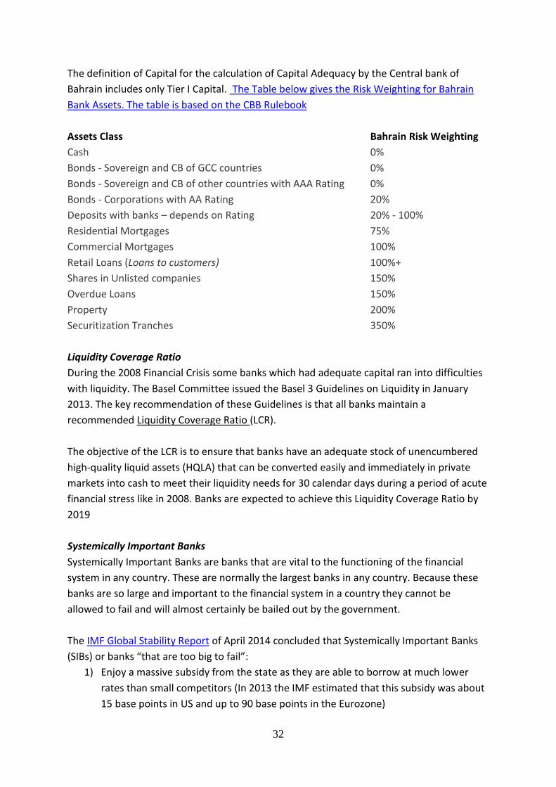
The definition of Capital for the calculation of Capital Adequacy by the Central bank of

Bahrain includes only Tier I Capital. The Table below gives the Risk Weighting for Bahrain

Bank Assets. The table is based on the CBB Rulebook

Assets Class Bahrain Risk Weighting

Cash 0%

Bonds - Sovereign and CB of GCC countries 0%

Bonds - Sovereign and CB of other countries with AAA Rating 0%

Bonds - Corporations with AA Rating 20%

Deposits with banks – depends on Rating 20% - 100%

Residential Mortgages 75%

Commercial Mortgages 100%

Retail Loans (Loans to customers) 100%+

Shares in Unlisted companies 150%

Overdue Loans 150%

Property 200%

Securitization Tranches 350%

Liquidity Coverage Ratio

During the 2008 Financial Crisis some banks which had adequate capital ran into difficulties

with liquidity. The Basel Committee issued the Basel 3 Guidelines on Liquidity in January

2013. The key recommendation of these Guidelines is that all banks maintain a

recommended Liquidity Coverage Ratio (LCR).

The objective of the LCR is to ensure that banks have an adequate stock of unencumbered

high-quality liquid assets (HQLA) that can be converted easily and immediately in private

markets into cash to meet their liquidity needs for 30 calendar days during a period of acute

financial stress like in 2008. Banks are expected to achieve this Liquidity Coverage Ratio by

2019

Systemically Important Banks

Systemically Important Banks are banks that are vital to the functioning of the financial

system in any country. These are normally the largest banks in any country. Because these

banks are so large and important to the financial system in a country they cannot be

allowed to fail and will almost certainly be bailed out by the government.

The IMF Global Stability Report of April 2014 concluded that Systemically Important Banks

(SIBs) or banks “that are too big to fail”:

1) Enjoy a massive subsidy from the state as they are able to borrow at much lower

rates than small competitors (In 2013 the IMF estimated that this subsidy was about

15 base points in US and up to 90 base points in the Eurozone)

33

2) May take excessive risks, as they are confident that they will be bailed out by the

state and these excessive risks may endanger the stability of the entire financial

system

3) Have become even more important as the Financial Crisis of 2008 led to industry

consolidation. Many countries have over 50% of bank assets controlled by three

banks.

The Global Financial Crisis of 2008 led to increased concern about SIBs and particularly G-

SIBs or Global-Systemically Important Banks. The G20, the club of the leading economies in

the world, set up the Financial Stability Board (FSB) in 2009.

The FSB and the Basel Committee on Bank Supervision have coordinated the global

response to SIBs. They have recommended:

1) Higher Capital Ratios for all SIBs

2) More Intense Supervision of all SIBs

The Basel 3 recommendations involve significantly higher Capital and Liquidity Ratios for

SIBs and many countries have even prescribed ratios even higher than Basel 3. Many Central

Banks, including the BoE and the ECB, have adopted new supervisory regimes with more

intense supervision of SIBs.

The Financial Stability Board has identified 30 large banks such as Goldman Sachs and HSBC

which are Global Systemically Important Banks. The FSB recommended in November 2014

that these Global SIBs be required to have Total Capital (Equity and Bonds) equal to 16% –

20% of Risk Weighted Assets.

Monetary Policy

Monetary policy, now often referred to a “Conventional Monetary Policy”, means the

control of interest rates and the value of a currency on the foreign exchange. In dealing with

Interest Rates it is useful to distinguish between the level of Interest Rates and the spread of

Interest Rates. These two topics are discussed below.

It is normally through the “Money Market” that the level of Interest Rates is established.

The “Money Market” is the market for unsecured short-term loans operated by the major

financial institutions. The interaction of Demand and Supply on the Money Market

determines the R of I for Short-Term Funds. The interest rate in the London Money Market

is called the Libor (London Interbank Offered Rate), the US rate is the Fed Funds Rate and

the Eurozone rate is the Euribor Rate. In normal times all other interest rates move in line

with Money Market rates although long-term rates tend to move less than short-term rates.

34

At any time Money Market Rates depend on the policy of the central bank and the level of

confidence in the currency. Central Banks have significant power to influence the R of I in

their economy. Central Banks try to control Money Market Rates through controlling the

amount of cash within the banking system and the rate of interest at which they lend for

short periods to the commercial banks and accept deposits.

The Central Bank of Bahrain, as of June 2014, was willing to lend to commercial banks at

2.25% and pays a rate of interest on 0.5% on deposits. This means that the Bahrain Money

Market rate cannot go above 2.25% or below 0.5%. If money market rates go above 2.25%

the commercial banks will borrow from the CBB and if money market rates go below 0.5%

the commercial banks will put their excess cash on deposit with the CBB.

Normally banks are able to borrow directly from each other for short periods through the

money market however the collapse of Lehman’s Bank in New York in 2008, the largest

bankruptcy in US history, led to a crisis of confidence in banking and a reluctance of banks to

lend to each other. What started to happen was that this money flooded into Central Banks

and short-term Government Bonds. Central Banks then lent the money to banks. This was

often referred to as “Emergency Liquidity Support”. The US Federal Reserve Bank, the Bank

of England and the ECB engaged in “Emergency Liquidity Support” in 2008 and 2009. In June

2009, for example, the ECB lent over €400 billion to Eurozone banks as part of this program.

The Federal Reserve System in the US was founded by Congress in 1913 “to provide the

nation with a safer, more flexible, and more stable monetary and financial system”.

Traditionally the US Federal Reserve Bank has attempted to control the Business Cycle in the

US Economy using the rate of interest.

The Fed controls the Money Market rate through its “Fed Rate” which is the Rate of Interest

on Reserves held by Commercial Banks with the Federal Reserve. Commercial banks borrow

and lend these Reserves between each other and the rate at which this money is traded is

the “Fed Rate”. The Fed sets a target for the “Fed Rate”.

The European Central Bank, which has been in control of interest rates in the Eurozone since

1999, has as its only/main target to keep inflation around 2%. The main rate of interest used

by the ECB to influence bank interest rates within the Eurozone is its Refinancing Rate or

“Refi Rate”. As the Great Recession developed the ECB gradually cut its Refi Rate to 0.25% in

2013 and then to 0.05% in 2014.

The level of confidence in a currency will influence Money Market rates. Confidence in a

currency is linked to the likelihood of devaluation. If there is a perception that a currency is

likely to be devalued, on the foreign exchanges, then any person who is able will try and

35

exchange the weak currency for other currencies and this will create a financial crisis and

drive up Money Market Rates.

The level of confidence in a currency is also linked to the level of inflation. If there is high

inflation the rate of interest will have to reflect this. The close link between inflation and

interest rates can be shown by international comparisons. High inflation countries have high

rates of interest and low inflation countries have low rates.

“Unconventional Monetary Policy”

The Financial Crisis in 2007/08 had such an impact on economies all over the World that

many central banks got involved in what is now called “Unconventional Monetary Policy”.

“Conventional Monetary Policy” involves adjusting short-term interest rates down to

manage overall demand in the economy. The difficulty with this policy is that it is very

difficult to push short-term interest rates much zero and the situation in 2007/08 warranted

negative short-term interest rates. This led central banks to start using “Unconventional

Monetary Policy”. Unconventional Monetary Policy involved using two new monetary policy

tools called “Quantitative Easing” and “Forward Guidance”.

The US Federal Reserve started a program of purchasing government bonds and asset-

backed securities at the end of 2008 when the US economy was plunging into deep

recession. “Quantitative Easing”, as it involves the central bank buying bonds and other

forms of securities, means that the amount of cash held by the banking system and the

public increases. (The term “Monetary Base” is used to describe the amount of cash held by

the public and the banks and the bank’s reserves with the central bank). Central banks

therefore make it easy for banks to increase their lending by Quantitative Easing (QE). QE

also increases the balance sheet of a central bank as it has paid out cash which is a liability

of the central bank and received in exchange a bond which is an asset.

Other central banks have also carried out large-scale asset purchase programs. The Bank of

Japan began a large-scale asset purchase program in 2009. In its most recent program,

launched in 2010, it has bought roughly $1.1 trillion in Japanese government bonds and

other assets. In March 2009, the Bank of England announced a “Large Scale Asset Purchase”

program and purchased $600 billion of assets (mostly of British government bonds).

The ECB did not use Quantitative Easing until Autumn 2014 because of German objections.

The Germans argued that increasing the money supply through Quantitative Easing would

lead to inflation.

The other “Unconventional Monetary Policy” tool is “Forward Guidance”. Central banks

were reluctant, up until the financial crisis in 2008, to give any advice about the future

direction of interest rates. Central banks did not want to limit their freedom to vary interest

36

rates by giving any clear statements on the future direction of rates. Since 2011, however,

the Fed has been using Forward Guidance as a tool of monetary policy. Forward Guidance

involves the Fed, or any central bank, giving a clear and transparent assessment of its

judgment on the direction of interest rates movement into the future.

The Fed has used Forward Guidance over the last few years to drive down medium-term

interest rates by signaling that they planned to keep short-term interest rates at a low level

for an extended period. When the Fed indicated that they were committed to keeping

short-term interest rates low for a considerable period it signaled to the market that there

was a much reduced risk to lenders for the medium term that they would be caught by a

rise in short-term rates. This helped to reduce medium term interest rates.

The BoE and the ECB have followed the lead of the Fed and also started using Forward

Guidance for the same purpose in recent years.

Inflation Targets

Most Central banks have an Inflation target of around 2%. Central banks have a fear of

deflation where the level of prices is falling. If prices are falling then persons and

organization are under no pressure to spend and may well postpone purchase decisions in

the expectation of lower prices in the future. If this happens then the level of overall

spending (demand) will be difficult to predict and may collapse. Central banks try to control

the level of overall demand by adjusting interest rates. This is very easy if prices are rising as

the level of interest rates can be adjusted to encourage or discourage spending. However if

prices are falling the most that a central bank can do is cut its interest rate to zero. This will

ensure that the rate of interest on bank deposits is also zero (or a little below). If prices are

falling persons who have money on deposit at zero interest rate are still making a profit as

they will be able to buy more in the future by leaving the deposits unspent. Deflation

therefore makes central bank interest rates largely useless as a way of controlling overall

demand in an economy. The Japanese experience with Deflation has shown how deflation

undermines that ability of a central bank to control overall demand and led the Japanese

Government and the Bank of Japan to agree on a 2% inflation target in 2013.

A small level of inflation has other attractions. It allows persons at work to look forward to

small annual wage increases. Inflation is also attractive to governments as almost all

governments are in debt (the national debt) and debts are gradually reduced in real terms

by inflation.

The benefits of a small level of inflation in terms of monetary policy, annual wage increases

and erosion of national debt has led to a consensus that an inflation target of around 2% is

appropriate.

37

Central Bank of Bahrain Glossary of Banking Terminology

The CBB Rulebook has a Glossary of Financial terms which may be useful. Some of these

financial terms are given below:

Base Rate and Prime rate

Base Rate is the interest rate that underpins lending to bank customers. Banks lend to their

customers at basis points over base rates. Prime Rate is the rate at which a bank will lend to

its most creditworthy customers

Basel Capital Accord Issued initially in July 1988 by the Basel Committee on Banking Supervision, the Basel Capital Adequacy Accord is a risk based capital adequacy methodology that defines the components of capital and applies a series of risk weights and capital charges to banks' assets and holdings of financial instruments. The Accord aims to increase the stability of the international financial system through having a single internationally acknowledged measurement of a bank's capital expressed as a percentage of its financial risks. It also serves to put internationally active banks on an equal competitive footing in respect of the measurement of their capital adequacy Bonds An instrument creating or acknowledging a present or future indebtedness (i.e. debentures, debenture stock, loan stock, bonds, certificates of deposit and any other instruments creating or acknowledging a present or future indebtedness), but excluding:

(a) An instrument creating or acknowledging indebtedness for, or for money borrowed to

defray, the consideration payable under a contract for the supply of goods and services;

(b) A cheque or other bill of exchange, a bankers draft or a letter of credit (but not a bill of

exchange accepted by a banker);

(c) A banknote, a statement showing a balance on a bank account, or a lease or other

disposition of property; and

(d) A contract of insurance

Capital adequacy

A measure of the financial strength of a bank or securities firm, usually expressed as a percentage ratio of its capital to its assets

Certificate of deposits This is a certificate issued by a bank or thrift that indicates a specified sum of money has been deposited with it for a specified period at a defined rate. A CD shows a maturity date and a specified interest rate, and can be issued in any denomination. The duration can be up to five years

Collateral Any form of property, security, guarantee or indemnity provided as security for a borrower.

Conventional bank license A license issued under Volume 1 of the CBB Rulebook. A Conventional bank license only allows a bank to take deposits and give credit.

38

Conventional wholesale bank licensee A conventional bank licensee, licensed as a wholesale bank Credit risk Is defined as the potential that a bank's borrower or counterparty will fail to meet its obligations in accordance with agreed terms. Credit risk exists throughout the activities of a bank in the banking book and in the trading book and includes on- and off-balance sheet exposures.

Dealing in financial instruments as agent Dealing in financial instruments as agent means buying, selling, subscribing for or underwriting any financial instrument on behalf of a client Dealing in financial instruments as principal Dealing in financial instruments as principal means buying, selling, subscribing for or underwriting any financial instrument on one's own account

Default Failure to service a credit in accordance with agreed terms, e.g. late or incomplete payments of principal or interest, or infringement of any other material provision of the credit documentation

Deposit: A contract that grants the bank the right to possess the deposited money and to dispose thereof in its ordinary course of business with an obligation to return an equal amount thereof to the depositor. Repayment of the deposit shall be in the same currency of the original deposit.

The definition of Deposit is more complex for a Sharia-compliant bank.

Derivative(s) A generic term for a financial instrument whose value is dependent on, or derived from, the changes in the absolute or relative value of some underlying asset or market index or rate. Often used for futures, options and swaps

Future(s) Rights under a contract for the sale of a commodity or property of any other description under which delivery is to be made at a future date and at a price agreed on when the contract is made

Going concern The idea that a company will continue to operate indefinitely, and will not go out of business and liquidate its assets.

Hedging A strategy designed to reduce investment risk using call options, put options, short-selling, or futures contracts. A hedge can help lock in profits. Its purpose is to reduce the volatility of

39

a portfolio by reducing the risk of loss.

Independent director An 'independent director' is a director whom the board has specifically determined has no material relationship which could affect his independence of judgment, taking into account all known facts.

Insider trading The activity which is in summary:

(a) The offence of which an individual is guilty if he has information as an insider and:

(i) In the circumstances described in (b), he deals in securities that are price-affected

securities in relation to the information; or

(ii) (A) he encourages another person to deal in securities that are (whether or not that other

knows it) price affected securities in relation to the information, knowing or having

reasonable cause to believe that the dealing would take place in the circumstances mentioned

in (b); or (B) he discloses the information, otherwise than in the proper performance of the

functions of his employment, office or profession, to another person; and

(b) The circumstances referred to in (a) are that the acquisition or disposal in question

occurs on a regulated market, or that the person dealing relies on a professional

intermediary or is himself acting as a professional intermediary

Islamic bank licensee

Liquidation The process of terminating a bank's activities whereby all creditors are discharged either in full (a solvent liquidation), or in part (an insolvent liquidation) and any remaining funds are returned to the shareholders. This process normally takes place in accordance with the requirements of specific legislation in the country of incorporation. In Bahrain this includes the Bankruptcy and Preventative Settlements Act.

Market risk The risk of losses in on- and off-balance sheet positions arising from movements in market prices. The risks that are subject to the market risk capital requirement are:

(a) Equity position risk in the trading book

(b) Interest rate risk in trading positions in financial instruments in the trading book

(c) Foreign exchange risk

(d) Commodities risk

Money-market instruments Those classes of instruments which are normally dealt in on the money market, such as treasury bills, certificates of deposit and commercial papers and excluding instruments of payment.

Option(s) An option is a contract giving the buyer the right, but not the obligation, to buy or sell any of the following at a specific price on or before a certain date:

(a) Currency of the Kingdom of Bahrain or any other country or territory;

(b) Palladium, platinum, gold or silver; or other commodity;

40

(c) Option to acquire or dispose of a financial instrument of the kind specified by this

definition by virtue of the above

Overseas conventional bank licensees Conventional bank licensees that are incorporated in an overseas jurisdiction and operate via a branch presence in the Kingdom of Bahrain

Over the counter (OTC) A decentralised market (as opposed to an exchange market) where geographically dispersed dealers are linked by telephones and computer screens. OTC trades are more often than not, denominated in non-standard amounts and on non-standard terms (eg maturity outside IMM dates). The term may also refer to trading in securities not listed on a stock or bond exchange.

Regulated banking services Any of the regulated activities permitted to be undertaken by a conventional bank licensee

Repo (a) an agreement between a seller and buyer for the sale of securities, under which the seller

agrees to repurchase the securities, or equivalent securities, at an agreed date and, usually, at

a stated price;

(b) an agreement between a buyer and seller for the purchase of securities, under which the

buyer agrees to resell the securities, or equivalent securities, at an agreed date and, usually,

at a stated price.Sovereign debt A debt instrument issued by central government.

Spot transactions

A foreign exchange transaction in which each party promises to settle the transaction two days after the transaction date

Swap(s)

A financial contractual agreement between two parties to exchange (swap) a set of payments that one party owns for a set of payments owned by the other party Underwriting A binding commitment by the reporting bank to purchase securities issued by, or provide syndicated loans/credit facilities to (as the case may be) an unconnected party ("the issuer" or "the borrower") at a mutually agreed price.

Wholesale BankWholesale banks are defined as banks who undertake the regulated banking

service of (a) and (b) plus any activity from (c) to (o) of those listed in AU-A.1.4 with

41

Commodity Markets

This section covers the variety of Market Types, Commodity Markets, Market Balance, Price

Instability, Elasticity, Market Stability, Minimum Prices, Price Cycles, the Price of Oil, the

impact of technology improvements on market prices and long term trends in food prices.

Variety of Market Types

There is an enormous variety of Market Types. Some Markets are local and others are

world-wide, some are real products and others are financial products, some are individual

products and others are entire systems, some are brands and others are commodities, some

are high technology and others are low technology, some have very few buyers or sellers

and others have many buyers or sellers.

Markets can be viewed from a variety of perspectives. All businesses are particularly

interested in the market in which they are selling their products. Sellers are interested in the

market price and understanding their ability to control their selling price. The ability to

control the market price is called Market Power. This analysis looks at markets from the

perspective of the seller and focuses on the seller’s Market Power.

42

There are three key factors that appear to influence the market power of a Seller in every

market. These are the number of competitors, the degree of product variation or

differentiation and the relationship with the customer.

The seller has massive market power if s/he is the only seller. The seller has increased

market power if her product meets the needs of the customer and her product is perceived

as being significantly different from alternatives. The relationship with the final customer is

also a key determinant of market power. If a seller has a close relationship with the final

customer based on understanding the customer’s needs in depth, an ability to meet these

needs precisely and trust from previous interactions this gives a high degree of market

power.

When markets are seen from the perspective of the seller and classified in terms of Market

Power three market types appear to dominate. These key market types are Monopoly

Markets, Brand Markets and Commodity Markets.

Monopoly Markets exist where there is only one seller and in this situation the Monopolist

has great market power. Companies which have developed Strong Brands have a degree of

Market Power similar to the Monopolist. These strong brands are based on product

differentiation and building a close relationship with the customer. The vast majority of

businesses however sell commodity type products in Commodity Type Markets and the

dominant form of trading, particularly in financial instruments, is in commodity type

markets.

Commodity Markets

Business and financial commentators use the term “Commodity Market” to refer to highly

organized physical commodity markets such as those for oil, metals including precious

metals and farm products. These markets, such as the Chicago Commodity Exchange and

the London Metals Exchange, trade in standardized products, have large numbers of buyers

and sellers and have significant involvement of middlemen including traders and brokers.

However modern financial markets are organized in exactly the same way with standardized

products, large numbers of buyers and sellers and significant involvement of middlemen

including traders and brokers. These markets can be described as Commodity-Type Markets.

A Commodity-Type Market exists where:

a) There are a large number of both Buyers and Sellers

b) The product is Standardised.

C) Middlemen control the Relationship with Customers

Commodity Markets are markets where no individual buyer or seller has any significant

ability to control the market price. For a market to be a commodity market there must be a

large number of buyers and sellers. If this is not the case then either the buyers or the

43

sellers can organize to dominate the market. For example if there are only 2 or 3 sellers it is

relatively easy for them to share the market and eliminate competition.

For a market to be a commodity market the product must be standardized or at least the

products of individual firms must be very similar. This applies to both technical features of

the product and product image. For a product to be a commodity the purchaser must not be

concerned about the identity of the producer. If a company is selling a technically

differentiated product with a particular image then it is likely that the purchaser will be

interested in the identity of the producer and the output of that producer will be identified

as a brand.

All commodity markets have middlemen who link producers and customers and control the

relationship with customers. Such middlemen include traders, wholesalers, dealers, agents

and brokers. Standardization makes it easier for middlemen to operate in a market and the

existence of middlemen encourages standardization.

These middlemen encourage product standardization as it makes it much easier for them to

trade if the products from different producers are standardized. For example in 1848 the

Chicago Commodity Exchange standardized the farm products that it traded in. This made it

easier for the traders, for example, to use the newly invented telegraph system to sell farm

products from a Mid-West US farmer to a London food importer. Before the emergence of

“marketing” and branding in the US from 1900 to 1930 most markets were dominated by

chains of middlemen and the producers did not control the relationship with customers.

One of the key challenges for the early companies in branding, such as P&G, was to

eliminate the middlemen and gain control of the customer relationship. It was only in this

way that the producer, eg P&G, could effectively guarantee the quality of its product to the

customer and build the relationship of trust that is fundamental to any brand.

The World Bank Commodity Price Database covers 70 physical commodities and gives prices

for many years, with some price series dating back to 1960.

Financial Commodity Markets include a wide variety of financial products such as Bonds, FX,

Equities and Derivatives. There has been a massive growth in trading in complex financial

products such as Derivatives and Asset Backed Securities over the last 40 years.

A derivative is a contract that derives its value from the performance of an underlying entity

such as an index eg S&P500.The growth of trading in these complex financial commodities

led the US to set up the US Commodity Futures Trading Commission in 1975 to regulate the

market.

Futures Trading in farm products was developed by the Chicago Board of Trade in the 1850s.

This allowed farmers to sell their products in advance and reduce risk. Futures Trading was

gradually extended to a whole range of physical products such as metals and energy. CME ,

the successor to the Chicago Commodity Exchange, which describes itself as the “world's

44

leading and most diverse derivatives marketplace” launched its first Financial Futures

product in 1971. This involved futures contracts based on 7 currencies priced in $s. In 1981

CME started offering futures contracts based on the S&P 500 Index and US Treasury Bonds.

CME now offers futures and options based on interest rates, equity indexes, foreign

exchange, energy and agricultural products.

Bloomberg's site classifies markets under Indexes, Futures, Currencies and Bonds. All of

these are financial products and all are sold in commodity-type markets. The Financial Times

e/edition gives market data under a variety of headings including Equities, Currencies,

Capital and Commodities. Three of these are financial products sold in commodity-type

markets.

Market Balance in Commodity Markets In

Commodity Markets the bargaining between Buyers and Sellers determines the price. An

example of a very simple situation will illustrate how price is determined.

The following 5 Buyers and 5 Sellers go into a market to trade a standardized item (the

number of Buyers and Sellers is too low for a Commodity Market but this is to make your

calculations easier).

A is willing to buy 2 units at a Price up to $13 per unit

B is willing to sell 3 units at a Price of $12 or more per unit

C is willing to buy 2 units at a Price up to $16 per unit

D is willing to buy 3 units at a Price up to $12 per unit

E is willing to sell 2 units at a Price of $15 or more per unit

F is willing to sell 2 units at a Price of $16 or more per unit

G is willing to buy 5 units at a Price up to $15 per unit

H is willing to sell 4 units at a Price of $13 or more per unit

I is willing to buy 2 units at a Price up to $14 per unit

J is willing to sell 2 units at a Price of $14 or more per unit

The market will balance at a price at which the amount that sellers want to sell (Supply) will

be equal to the amount that buyers want to buy (Demand). The way to calculate the price at

which supply and demand balances is to calculate the amount for sale at all different price

and the amount demanded at all different prices. These calculations are easier if you start

calculating supply from a low price and calculating demand from a high price. The number

of units that are for sale (supply) at all the different prices is shown below,

Market Price $1 Sellers - Units for sale 0

Market Price $12 Sellers B Uni1ts for sale 3

Market Price $13 Sellers B,H Units for sale 7

Market Price $14 Sellers B,H,J Units for sale 9

Market Price $15 Sellers B,H,J,E Units for sale 11

Market Price $16 Sellers B,H,J,E,F Units for sale 13

45

The number of units that buyers wish to buy (demand) at all the different prices is shown

below,

Market Price $17 Buyers - Units demanded 0

Market Price $16 Buyers C Units demanded 2

Market Price $15 Buyers C,G Units demanded 7

Market Price $14 Buyers C,G,I Units demanded 9

Market Price $13 Buyers C,G,I,A Units demanded 11

Market Price $12 Buyers C,G,I,A,D Units demanded 14

Market Price $11 Buyers C,G,I,A,D Units demanded 14

The market will balance at a price that makes supply equal to demand. This price will allow

all market participants who wish to buy or sell at the market price to do so. In this case the

price will fix at $14 and B, H and J will sell 9 units to C, G and I. The way the market is

brought into balance or equilibrium by the price is normally represented by the diagram

below.

Supply and Demand Curves

Supply Curve

Demand Curve

Units

The price that balances supply and demand is often called “the equilibrium price” because it

brings balance to the market. The equilibrium price is the price that ensures that the

quantity that sellers want to sell is the same as the quantity that buyers want to buy (supply

= demand).

The sensitivity of a market to changes in supply or demand can be illustrated by working out

the impact of a new trader entering the above market. If this new trader wishes to sell 4

units at a price at or above $11 the market price will fall from $14 to $13 but if he wishes to

buy 4 units at a price at or below $16 the market price will rise to $15.

Price Instability

The nature of commodity markets means that prices are unstable. In brands markets and

monopoly markets the firm that is selling sets the market price and brings stability to the

market.

Equilibrium

Price

46

In commodity markets the price is determined by the interaction of Supply and Demand and

prices constantly fluctuate, even minute by minute as in financial markets, as Supply and

Demand conditions change. Commodity markets are also influenced by speculation as

buyers buy in anticipation of price increases and sellers sell in anticipation of price falls.

The graph below gives the price of silver in $ per Troy Ounce. The 1980 spike in silver prices

is believed to have been largely the result of speculation, particularly by the Bunker Hunt

family who set out to control the world silver market in the late 1970s. This drove silver

prices from below $1 per ounce in the 1960s to almost $40 per ounce.

Price of Silver in Current $s per Troy Ounce from 1960 to 2015

Source, World Bank GEM Series – “Pink Sheets” World Bank Commodity Prices

The price of Gold also shows massive variation over the last 50 years but has been more

stable than Silver.

0.00

5.00

10.00

15.00

20.00

25.00

30.00

35.00

40.00

45.00

60

65

70

75

80

85

90

95

0 5 10

15

Silver

Silver

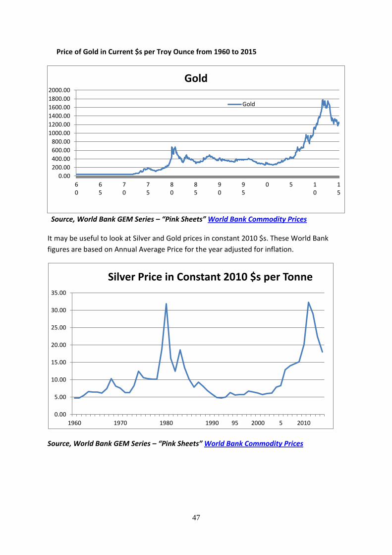
47

Price of Gold in Current $s per Troy Ounce from 1960 to 2015

Source, World Bank GEM Series – “Pink Sheets” World Bank Commodity Prices

It may be useful to look at Silver and Gold prices in constant 2010 $s. These World Bank

figures are based on Annual Average Price for the year adjusted for inflation.

Source, World Bank GEM Series – “Pink Sheets” World Bank Commodity Prices

0.00

200.00

400.00

600.00

800.00

1000.00

1200.00

1400.00

1600.00

1800.00

2000.00

60

65

70

75

80

85

90

95

0 5 10

15

Gold

Gold

0.00

5.00

10.00

15.00

20.00

25.00

30.00

35.00

1960 1970 1980 1990 95 2000 5 2010

Silver Price in Constant 2010 $s per Tonne

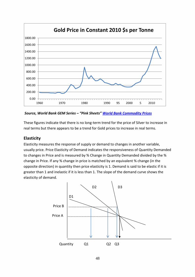
48

Source, World Bank GEM Series – “Pink Sheets” World Bank Commodity Prices

These figures indicate that there is no long-term trend for the price of Silver to increase in

real terms but there appears to be a trend for Gold prices to increase in real terms.

Elasticity

Elasticity measures the response of supply or demand to changes in another variable,

usually price. Price Elasticity of Demand indicates the responsiveness of Quantity Demanded

to changes in Price and is measured by % Change in Quantity Demanded divided by the %

change in Price. If any % change in price is matched by an equivalent % change (in the

opposite direction) in quantity then price elasticity is 1. Demand is said to be elastic if it is

greater than 1 and inelastic if it is less than 1. The slope of the demand curve shows the

elasticity of demand.

D2 D3

D1

Price B …………………………….………………..

Price A ……………………….……………………….

Quantity Q1 Q2 Q3

0.00

200.00

400.00

600.00

800.00

1000.00

1200.00

1400.00

1600.00

1800.00

1960 1970 1980 1990 95 2000 5 2010

Gold Price in Constant 2010 $s per Tonne

49

In the diagram above D1 represent very elastic demand as any % change in price will lead to

a much greater % change in quantity. D2 represent a price elasticity of around 1 and D3

represents an inelastic demand.

The elasticity of supply can be measured in exactly the same way. Price Elasticity of Supply

indicates the responsiveness of quantity supplied to changes in price and is measured by %

change in Q divided by % change in P. If the % change in price is matched by a

corresponding % change in quantity supplied then the price elasticity of supply is 1 (S2). If

the figure is above 1 it is said to be elastic (S3) and if below 1 then it is said to be inelastic

(S1)

The key factors that influence Elasticity of Supply (the shape of the supply curve) are

Industry Capacity and Variable Cost per Unit.

If the market price in a commodity market is at or above Total Cost per Unit then all firms

will supply at close to their capacity. In some industries a very high price will not lead in the

short run to a significantly higher level of supply because of capacity constraints. This means

that the Supply Curve will rise almost vertically when volume approaches Industry Capacity

(S1). In other industries it may be easy to increase capacity so the supply curve will be like

S3.

Every firm will have some Fixed Costs so it will make sense, in the short run, for a firm to sell

at a market price just below its Total Cost per Unit as it will be reducing its losses or making

a Contribution to Overheads. It will not, however, make sense for a firm to sell at a market

price below its Variable Cost per Unit so supply on to any commodity market will reduce

significantly if the market price drops below Variable Cost per Unit.

The structure of costs in any industry will significantly influence the level of stability of an

industry. Some industries have very high Fixed Costs and low Variable Costs. Other

industries have low Fixed Costs and high Variable Costs. Industries with high Fixed Costs are

likely to be unstable whereas industries with high Variable Costs are likely to be stable. The

oil industry is an example of an industry with high Fixed Costs and low Variable Costs. The

capital costs (Fixed) to open up a new oil well are very high but then the operating (Variable)

costs are low. This is part of the reason for the instability of the oil market.

Market Stability and Elasticity

The stability of price in any commodity market is linked to the price elasticity of supply and

demand. If both supply and demand are elastic then the price will tend to be very stable as

any disturbance to either supply or demand will not change price significantly. This is

represented by Diagram A below. If both supply and demand are inelastic then the price will

tend to be very unstable as any disturbance to either supply or demand will change price

significantly. This is represented by Diagram B below.

50

A, Elastic Supply and Demand Diagram B, Inelastic Supply and Demand

D1 D2 D1 D2

Price 1 …………………………………… ………………………………………………………………..……………..

Units Units

The relationship between demand and supply elasticity and price stability is illustrated by

the two diagrams above. Diagram A illustrates a situation where both demand and supply

are elastic. In this situation an increase in Demand, represented by a shift in the demand

curve from D1 to D2, leads only to a modest increase in price to P2. Diagram B represents a

situation where both demand and supply are inelastic. In this situation an increase in

Demand, represented by a shift in the demand curve from D1 to D2, leads to a dramatic

increase in price to P3. The world oil market is an example of a market with very inelastic

supply and demand. This results in a very unstable prices and massive fluctuations in profit

margins. The egg market on the other hand is an example of a market with elastic supply

and elastic demand and this results in relative stability of prices.

Minimum Prices

If there is over-supply, relative to demand, in any market that market will only come into

balance if suppliers reduce sales and in some cases if suppliers cease production. The price

will have to fall to drive the excess production out of the market. If there is, for example,

10% over-supply then the price must fall sufficiently to drive 10% of production out of the

market (assuming no increase in demand).

All businesses will have Fixed Costs or Overheads and Variable Costs. Fixed Costs or

Overheads are costs that the business must meet irrespective of its level of production or

sales as long as it continues to operate. Examples of Fixed Costs are Rates, Bank

Repayments, Depreciation of Plant and Machinery. Variable Costs are costs that vary with

the level of production and sales. Examples of Variable Costs are Raw Materials, Energy and

Direct Labour Costs. The Variable Cost per unit is the extra cost of producing one more unit

and will obviously reflect the amount of extra raw materials, energy and other inputs

needed to produce one extra unit.

If there is over-supply in a commodity market the price will have to fall to reduce supply.

Companies supplying to a Commodity Market will usually continue to supply while they are

covering their Variable Cost per Unit. In an over-supply situation therefore the price will fall

51

to just below the Variable Cost per Unit of the most inefficient producers. This should drive

sufficient production capacity out of the industry to bring about balance between supply

and demand.

The price of Zinc fell from over $1,550 per tonne in 1990 to $800 in 2002. This price fall had

an enormous impact on the profitability of mining companies such as Tara Mines, Europe’s

largest lead/zinc mine. Tara Mines closed temporarily in 2003 as a result of the fall in the

price of zinc. Widespread closures in any industry will eliminate over-supply and bring the

market back into balance. The price of zinc rose with the recovery in the World economy

and exceeded $3k per tonne in 2006/07.

Source, World Bank GEM Series – “Pink Sheets” World Bank Commodity Prices

The above chart is based on current prices for zinc but a better insight into the market can

be got by looking at zinc prices in constant prices. This data is also available from the World

Bank GEM series. The chart below gives zinc prices per tonne in constant 2010 $ but is

based on Annual Average Prices whereas the Chart above is based on Monthly Average

Prices.

0.00

500.00

1000.00

1500.00

2000.00

2500.00

3000.00

3500.00

4000.00

4500.00

5000.00

60

65

70

75

80

85

90

95

0 5 10

15

Zinc Prices in Currrent $ per Metric Tonne

Zinc

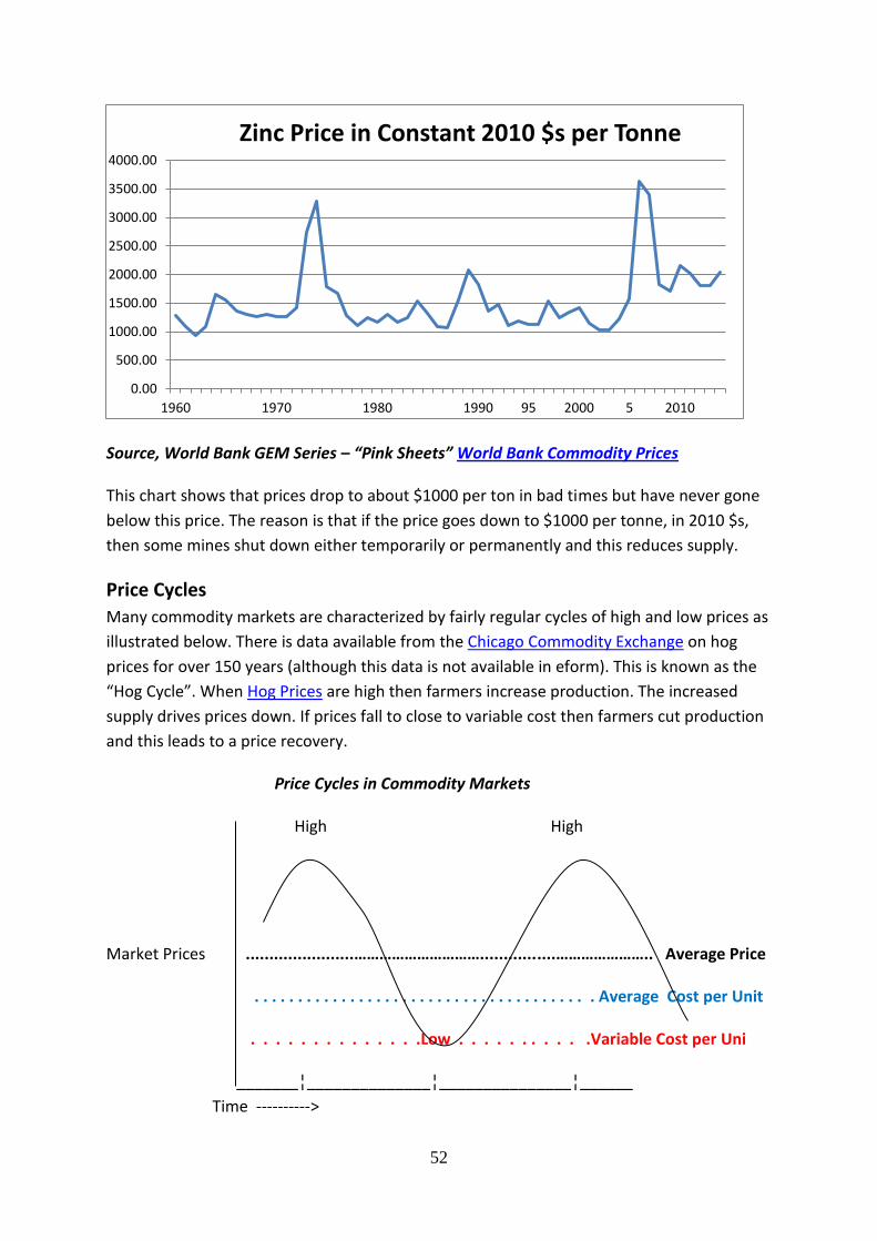
52

Source, World Bank GEM Series – “Pink Sheets” World Bank Commodity Prices

This chart shows that prices drop to about $1000 per ton in bad times but have never gone

below this price. The reason is that if the price goes down to $1000 per tonne, in 2010 $s,

then some mines shut down either temporarily or permanently and this reduces supply.

Price Cycles

Many commodity markets are characterized by fairly regular cycles of high and low prices as

illustrated below. There is data available from the Chicago Commodity Exchange on hog

prices for over 150 years (although this data is not available in eform). This is known as the

“Hog Cycle”. When Hog Prices are high then farmers increase production. The increased

supply drives prices down. If prices fall to close to variable cost then farmers cut production

and this leads to a price recovery.

Price Cycles in Commodity Markets

High High

Market Prices .......................…………………………................………………….. Average Price

. . . . . . . . . . . . . . . . . . . . . . . . . . . . . . . . . . . . . . . Average Cost per Unit

. . . . . . . . . . . . . .Low . . . . . . . . . . .Variable Cost per Uni

_______¦______________¦_______________¦______

Time ---------->

0.00

500.00

1000.00

1500.00

2000.00

2500.00

3000.00

3500.00

4000.00

1960 1970 1980 1990 95 2000 5 2010

Zinc Price in Constant 2010 $s per Tonne

53

The diagram below gives the price of Arabica Coffee Beans in terms of constant $s per kg for

the last 53 years. The coffee bean market, where producers interact with purchasers of

coffee beans, is a commodity market although when the product is sold to the consumer it

usually is a branded market. The price of coffee beans is determined by supply and demand.

The chart shows massive instability in price. This is largely due to variations in the quantity

supplied to the market. If supply is scarce then the price rises significantly. If there is

oversupply then the price will drop dramatically. The Demand for coffee is inelastic and this

means that the variation in supply from time to time cause massive price fluctuations.

Source, World Bank GEM Series – “Pink Sheets” World Bank Commodity Prices

The Price of Oil

0.00

2.00

4.00

6.00

8.00

10.00

12.00

1960 1970 1980 1990 2000 2010

Arabica Coffee Price in Constant 2010 $ per KG

The price of Crude

Oil has fluctuated

enormously over the

last 50 years. This is

illustrated by the

diagram below which

is taken from the

World Bank data for

monthly average oil

prices per barrel at

Dubai in current $s.

54

Oil is traded in units of barrels (BBL) because in the early years of the industry oil was

transported in wooden barrels. A barrel of oil has about 160 litres. The price is usually

measured in $s per barrel.

Source, World Bank GEM Series – “Pink Sheets” World Bank Commodity Prices

The price of crude oil fluctuated between 1$ and $3 per barrel from 1945 to 1973. A

reduction in supply, organized by OPEC (Organisation of Petroleum Exporting Countries), led

to an increase in price to above $37 for a period in 1980. This high price led to increased

supplies and reduced demand forcing prices down. There was a price spike in 1991 after the

invasion of Kuwait by Iraq. The price of oil held close to $15 from 1992 to 1996 but fell to

below $10 per barrel in for a short period in 1997. OPEC attempted to keep the price close

to $20 from 2000 to 2003.

Increased demand in recent years combined with the threat to supply linked to the US

invasion of Iraq in 2003 pushed prices above $70 in 2005 and up to $100 in December 2007.

The price continued to rise in Spring 2008 and reached $147 per barrel before falling back to

below €32 in December 2008. The price of oil rose again to reach $80 per barrel in

November 2009. The price of oil remained relatively steady from 2010 to 2014 about $100

per barrel before dropping dramatically to around $50 at the end of 2014. (The prices in the

charts are average annual prices so they do not fully indicate the level of price fluctuation)

If these oil prices are adjusted for inflation, as in the next table, a significantly different

pattern emerges. It now (2015) takes $5 to purchase what $1 purchased in 1960 so the

$1.50 per barrel price in 1965 is the equivalent of $7.50 now.

0.00

20.00

40.00

60.00

80.00

100.00

120.00

140.00

60

65

70

75

80

85

90

95

0 5 10

15

Oil price at Dubai in Current $s per barrel

Oil

55

Source, World Bank GEM Series – “Pink Sheets” World Bank Commodity Prices

These price fluctuations are caused by imbalances between supply and demand. The

demand for oil is fairly stable in the short term and has generally tended to grow over this

period. The demand for oil however, is very inelastic and this creates price instability if

supply fluctuates.

World Market for Oil in millions of barrels per day

150$ D

S

100$

30$

| | | | | | | | | | |

0 10 20 30 40 50 60 70 80 90 100

The above diagram, which attempts to represent the world oil market, shows a very

inelastic demand and very inelastic supply. The inelastic demand means that a scarcity could

0.00

20.00

40.00

60.00

80.00

100.00

120.00

1960 1970 1980 1990 2000 2010

Annual Average Oil Price at Dubai in Constant 2010 $s per Barrel

56

easily drive the price to $150 or a surplus could drive the price down to close to $30. The

variable costs in the industry are such that even if the price fell to $30, many suppliers

would continue to supply.

Over the past 30 years there have been massive variations in the price of crude oil but these

price variations have not, in the short term, led to major changes in demand, which has

tended to grow slowly, because energy usage is built into the pattern of living of people.

OPEC estimated that total crude oil production ran at about 92 million barrels per day in

2014 and this is gave a market balance at just around $90 per barrel. The US Energy

Information Agency information gives detailed breakdowns of energy usage by country.

Technological Improvements

If there are improvements in technology that allow a reduction in costs this will inevitably

be reflected in the market price especially if the industry is competitive. The massive

reduction in transport costs over the last 200 years has been a major factor in encouraging

an increased scale of production. Another industry showing massive cost reductions is

computing. The Computing Power provided by a $1,500,000 mainframe computer in 1970 is

now provided by a $400 laptop. This has happened as technological development cut

production costs and competition forced prices down in step with the reduction in costs as

effectively the PC market became a commodity type market.

The Computing Market from 1970 to 2014

D 70

1970 Price S 70

D 14 S 14

2014 Price ___|_______________________________________________________

1970 Units Q2014

D70 = 1970 Demand Curve, S70 = 1970 Supply Curve, D 14 = 2014 Demand Curve, S 14 =

2014 Supply Curve. (Diagram not to Scale)

Long-term trends in World Food Prices

The World Bank has collected data on World Food prices for over 50 years. Three of the key

food products are Soyabean, Wheat and Rice and these prices are given in the two charts

below.The data for the first chart is the Monthly Average Price in Current $s. This shows a

high level of price fluctuation. The second chart gives the Average Annual Price in Constant

2010 $s and as these are annual averages the price fluctuation is much less.

57

The spike in prices in the mid-1970s was linked to higher energy prices which led farmers to

use less fertilizer and this reduced crop yields. The World demand for these crops does not

change significantly from year to year, although it grows in line with population and income

growth, and therefore the significant price variation is largely caused by supply changes. The

second chart indicates a clear trend towards lower prices for these crops in real terms from

1960 to 2000 but that trend has changed in the last decade as the prices of these products

have risen significantly in real terms.

Price of Soyabean, Wheat and Rice per Metric Tonne in Current $s

Annual Average Price of Soyabean, Wheat and Rice in constant $2010 per Metric Tonne

Main Source, World Bank GEM Series – “Pink Sheets” World Bank Commodity Prices

0.00

100.00

200.00

300.00

400.00

500.00

600.00

700.00

800.00

900.00

1000.00

60

65

70

75

80

85

90

95

0 5 10

15

Soyabean

Wheat

Rice

0

200

400

600

800

1000

1200

1400

1600

1960 1965 1970 1975 1980 1985 1990 1995 2000 2005 2010 2015

Soyabean

Wheat

Rice

58

Macro-Economics or “Keynesian Economics”

Introduction

This note covers the Circular Flow of Income, Cycles in the Overall Economy, Wall Street

Crash of October 1929, impact of the Wall Street Crash outside the US, reaction of

Governments to the Wall Street Crash, Keynesian Analysis of a Simple Economy, Analogy of

a lake, More Complex Economy, Case Study of a Eurozone Boom, Financial Crisis of 2008/09

(The Great Recession) and the Great Depression in the US and the Great Recession in the

Eurozone PIIGS.

Circular Flow of Income

In a money-based economy Expenditure (Spending) purchases Sales. Sales and Production

are coordinated by business managers. Production generates Income as everybody who

contributes to production gets paid. Income finances Expenditure as people use their

income to buy the goods and services that they require. This is called the “circular flow of

income”. This relationship is very obvious with Services where for example when a person

spends BD20 on having a tooth filled the dentist has sales of BD20, valuing the production at

BD20, generating an income of BD20 for the dentist, who then has BD20 for spending. This

can be represented by

Expenditure of BD20 = Sales of BD20 = Production of BD20 = Income of BD20

Expenditure of BD20

This sequence should continue indefinitely as a circular flow of income but for the last two

centuries, recurring cycles of Boom and Recession have been observed and measured. A

Recession is normally defined as two quarters of falling Real GDP. A Depression is a

prolonged period of falling Real GDP.

Cycles in the Overall Economy

Trade Cycles or Business Cycles have been recorded for over 200 years. Between 1790 and

1914 Britain experienced 15 cycles. The longest of these cycles lasted for 11 years and the

shortest lasted for 5 years. Factors such as WW1, WW2 and Government Intervention in the

Economy during the 1950s and 1960s meant that the pattern and regularity of the Cycle was

distorted over most of the period from 1914 to 1970 but the pattern has become re-

established with recessions in Britain in 1974/75, 1982/83, 1991/92, 2001/2 and 2008/10.

In some of these “recessions”, such as the 2001/02 recession, most countries experienced a

drop in the growth rate but not a decline in real GNP. The most recent recession, now

referred to as the Great Recession, led to a fall in Real GNP in many countries

59

Over the period 1854 to 2009 the US experienced 33 Business Cycles according to the

National Bureau of Economic Research. The average length of these cycles was about 4.5

years with the shortest being 3 years and the longest being 11 years. The longest business

cycle in the last 150 years in the US was the cycle from 1991 to 2001. During this 11 year

cycle there were 10 years of continuous expansion. The longest period of contraction was

the 4 years of the Great Depression which followed the Wall Street crash of 1929. The Chart

below gives the Annual US GDP Growth Rates (Real) from 1930 to 2014.

US Bureau of Economic Analysis

Wall Street Crash of October 1929

In the period after the Wall Street Crash of October 1929 there was a major decline in share

prices with the Dow Jones Index (NYSE) falling from 381 to 41 (down 89%) between

September 1929 and June 1932. There was also a major decline in property prices. The

decline is asset prices led to a major loss of confidence and consumer demand fell. This led

to a situation where sales fell and businesses found that their level of stocks rose rapidly.

The increase in Stocks led to a cash-flow crisis and firms had to cut back both on their

production and investment. Many businesses went bankrupt as the recession developed.

The recession was then further aggravated by a financial crisis in which 9k of the 25.6k US

banks collapsed (1929 to 1933), wiping out the savings of millions. When a US bank went bankrupt the depositors lost access to their money for a period but in most cases the bank was taken over by another bank and the depositors, on average, received about 80% of their savings.

-15

-10

-5

0

5

10

15

20

25

30 40 50 60 70 80 90 0 10

US Annual GDP% Growth from Previous Year

GDP∆%

60

Unemployment rose from 3% in 1929 to 25% in 1933. Rising unemployment and the

collapse of businesses further eroded confidence and the US economy went into a

downward spiral which caused its Real GNP to fall by 33% between 1929 and 1933. The lack

of demand (Deflation) caused consumer Consumer Prices to fall by 21% between 1928 and

1934 . (Over this period farm prices fell by 50%). The combination of falling Real GNP and

falling prices caused GNP in Current Prices to fall by 46%.

There is still no full agreement on what caused the Wall Street Crash. Three important

factors which contributed to the crash are the level of Stock Market Speculation over the

period 1926 to 1929, the increase in interest rates and the introduction of tariff protection.

The Dow Jones Share Index rose from 100 in 1926 to 381 in September 1929. The rapid rise

in share prices was driven by a booming economy, new technology such as radio and high

levels of confidence. Rapidly rising share prices encouraged speculation, including share

purchasing “on margin”, and created a share “bubble” and a highly unstable situation.

The US was on the Gold Standard during the 1920s. In 1928 there was an outflow of gold

from the US particularly to France. The Federal Reserve Bank responded to this outflow by

increasing its Discount Rate (Lending Rate) from 3.5% in July 1928 to 6% in August 1929.

Increased interest rates usually drive down asset prices so the increase in interest rates was

a major contributory factor to the crash in share prices.

During the late 1920s US farmers campaigned for tariff protection. During the Presidential

Election campaign of 1928 President Hoover promised tariff protection for farmers, who

were suffering from depressed food prices, but as the bill passed through the House and

Senate its scope was significantly widened. The Smooth-Hawley Tariff Act as it is called,

increased average tariff levels on imports from 26% to 50% ad valorem. The act was being

debated in the Senate in October 1928 and it became obvious to investors that it would

become law. The act was finally signed into law by President Hoover in June 1930.

The Smoot-Hawley Tariff Act provoked a world-wide storm of retaliatory protectionism

which, in combination with the world recession, resulted in a 66% decline in world trade by

the mid-1930s, damaging business confidence and also damaging international relations.

The Smooth-Hawley Tariff Act is sometimes blamed for causing the depression but it

certainly made it worse.

The impact of the Wall Street Crash outside the US

The Wall Street Crash precipitated a world-wide recession and this recession was

particularly severe in Germany. Despite difficult problems including high “Reparations”

linked to the Versailles Treaty and the French occupation of the Ruhr in 1922 which

triggered the hyperinflation of 1923, the German economy was running smoothly in 1929.

61

There were active Communist and Nazi parties but they only commanded limited political

support. The Nazi Party, for example only got 2.6% of the vote in the 1928 election.

In the aftermath of the Wall Street crash the German economy went into a dramatic

recession which saw 5 major banks and over 20,000 businesses collapse. The recession led

to a rapid rise in unemployment, from 0.6 million in 1928 to 6 million in 1933. The recession

and banking collapse also wiped out the wealth and saving of millions of middle class

Germans. This changed the political situation dramatically. The Nazis increased their support

to 33% of the vote in November 1932 and Hitler was elected Chancellor in January 1933.

Reaction of Governments to the Wall Street Crash

The study of Trade Cycles, and the appropriate reaction of Governments, became the

central focus of Economics during the early 1930s as Economists and Politicians grappled

with a massive and world-wide economic recession. The conventional wisdom was that

governments should intervene to the minimum in the economy and balance their budgets.

The US Authorities, including the Federal Reserve Banks, stood by and allowed 40% of US

banks to go bankrupt. The NY Federal Reserve Bank even increased its Discount Rate (the

rate at which it made loans available to commercial banks) from 1.5% to 3.5% during 1930.

Governments all over the world found that as the recession developed that their tax

revenues fell substantially. Governments all over the world tried to balance their budgets by

increasing tax rates and reducing expenditure. The US had run substantial budget deficits in

1917 and 1918 to pay for WW1 but over the 1920s the Federal Government Budget was in

surplus. However in 1931 the budget went into deficit as tax revenues fell sharply. In

reaction the US increased income tax rates substantially with the top rate of Federal Income

Tax increasing from 25% to 79% between 1931 and 1936.

Keynes challenged the conventional wisdom in his writings over the early 1930s arguing that

these actions of governments were actually making the situation worse. The modern

understanding of Trade Cycles, which is called Macro-economics, is based on the work of JM

Keynes who published his “ General Theory” in 1936. The diagram below is based on a very

simplified approach to Keynes’s theory.

Version 1 (Explanation of Keynesian Economics using ordinary language)

Total Purchases of Goods and Services

Two sides of the one coin Sales and Purchases are identical for

each individual transaction. So Total

Purchases and Total Sales must be equal

Total Sales of Goods and Services

Businesses try to ensure that Sales If there is a difference

62

and Production are matched so Between Sales and Production then

Total Sales and Total Production Stock levels (Inventory levels) change

must be close

Total Production of Goods and Services

Production generates Income Almost identical but delays in calculating

and distributing Income

Total Income

People spend their Income Most Income will be spent but spending

and Total Demand is affected by a

variety of factors

Total Purchases of Goods and Services

If we look at this analysis we can see that there should be a rough balance between Total

Purchases (Spending) and Production but there can be imbalances. If there is too little

spending there will not be enough goods being purchased to keep pace with production so

businesses will have produced or purchased goods that they cannot sell. This will create

difficulties for business and will lead to a reduction in production causing lower

employment, lower income and further reductions in spending. This is the way that

recessions develop. If there is too much spending it will not be possible for business to

produce as much as they can sell and this will cause scarcity and price rises.

Version 2 (Explanation of Keynesian Economics using the language of Economics)

Simple Economy

In a Modern Economy the relationships between Expenditure, Sales, Production and Income

are very complex and this makes it difficult to understand what is happening. It is therefore

very useful to simplify and look at a situation where there is:

no Government

no International Trade and

no delays in Distributing Income.

If there is no Government there will not be any taxes, subsidies or welfare payments. Where

there are indirect taxes the seller does not get as much revenue as the purchaser spends.

Subsidies means that the producer receives more than is spent by consumers. Welfare

payments generate income for persons who do not earn it through the production of

goods/services.

If there is no International Trade then all trade is within this economy and all purchases in

the country must be balanced by sales in that country.

63

The assumption that there is no delay in Distributing Income means that when any product is

produced that instantaneously an equivalent amount of income arises. This situation is

approximated in the case of many services such as our example of dental services at the

start of this note. However in many situations this is unrealistic in that many goods take

months or even years to finish and there are often delays in the calculation of income

(company accounts) and payment of income. The distribution of profit is particularly slow.

We will call the economy where these conditions hold a “Simple Economy”.

Simple Economy

In this “Simple Economy” Total Production will be equal to Total Income because in such an

economy you can only get an Income from Production (there is no welfare provision) and

there is no delay in Distributing Income (assumption). Therefore Total Production (Y) €100 =

Total Income (Y) €100.

Savings and Investment

The relationship between Savings and Investment is crucial in determining how an economy

operates. We can work out how Savings and Investment are related in this Simple Economy

by analyzing Total Production (Y) and Total Income (Y).

Total Production or Y = Total Sales of Consumer Goods and Services ( C ) plus

Total Sales of Investment Goods ( I ) plus or minus

Stock Changes (Inventory changes) ( St )

Y = C + I ± St

(Note here that the word Stocks has a completely different meaning to the word when used

in discussing Stocks and Shares and is the same as Inventory in US English)

In this Simple Economy people will have only two choices about using their Income, either

to spend it by Purchasing Consumer Goods and Services or to Save it.

Total Income or Y = Total Purchases of Consumer Goods and Services or Consumption (C)

plus Total Savings (S).

Y = C + S

Total Production or Y = Total Income or Y (This was discussed above), therefore

C + I ± St = C + S

The C which represents Total Sales of Consumer Goods and Services must be the same as

the C which represents Total Purchases of Consumer Goods and Services, therefore

I ± St = S.

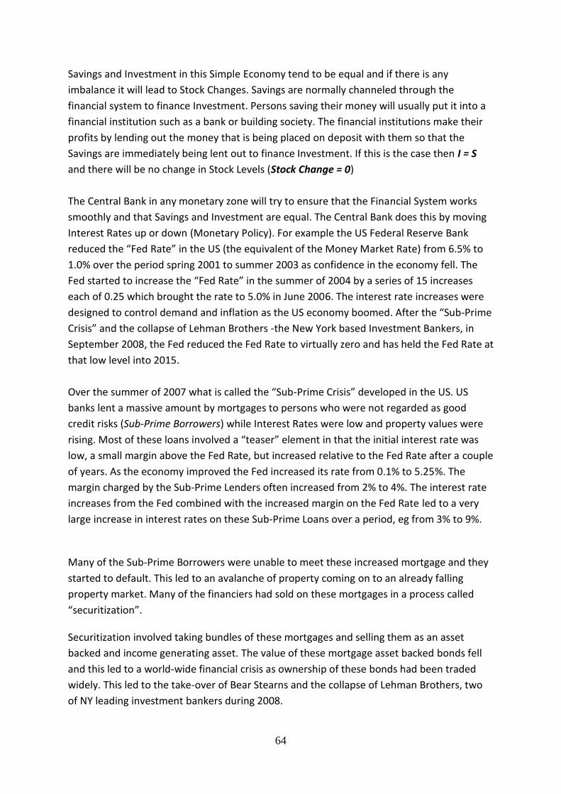
64

Savings and Investment in this Simple Economy tend to be equal and if there is any

imbalance it will lead to Stock Changes. Savings are normally channeled through the

financial system to finance Investment. Persons saving their money will usually put it into a

financial institution such as a bank or building society. The financial institutions make their

profits by lending out the money that is being placed on deposit with them so that the

Savings are immediately being lent out to finance Investment. If this is the case then I = S

and there will be no change in Stock Levels (Stock Change = 0)

The Central Bank in any monetary zone will try to ensure that the Financial System works

smoothly and that Savings and Investment are equal. The Central Bank does this by moving

Interest Rates up or down (Monetary Policy). For example the US Federal Reserve Bank

reduced the “Fed Rate” in the US (the equivalent of the Money Market Rate) from 6.5% to

1.0% over the period spring 2001 to summer 2003 as confidence in the economy fell. The

Fed started to increase the “Fed Rate” in the summer of 2004 by a series of 15 increases

each of 0.25 which brought the rate to 5.0% in June 2006. The interest rate increases were

designed to control demand and inflation as the US economy boomed. After the “Sub-Prime

Crisis” and the collapse of Lehman Brothers -the New York based Investment Bankers, in

September 2008, the Fed reduced the Fed Rate to virtually zero and has held the Fed Rate at

that low level into 2015.

Over the summer of 2007 what is called the “Sub-Prime Crisis” developed in the US. US

banks lent a massive amount by mortgages to persons who were not regarded as good

credit risks (Sub-Prime Borrowers) while Interest Rates were low and property values were

rising. Most of these loans involved a “teaser” element in that the initial interest rate was

low, a small margin above the Fed Rate, but increased relative to the Fed Rate after a couple

of years. As the economy improved the Fed increased its rate from 0.1% to 5.25%. The

margin charged by the Sub-Prime Lenders often increased from 2% to 4%. The interest rate

increases from the Fed combined with the increased margin on the Fed Rate led to a very

large increase in interest rates on these Sub-Prime Loans over a period, eg from 3% to 9%.

Many of the Sub-Prime Borrowers were unable to meet these increased mortgage and they

started to default. This led to an avalanche of property coming on to an already falling

property market. Many of the financiers had sold on these mortgages in a process called

“securitization”.

Securitization involved taking bundles of these mortgages and selling them as an asset

backed and income generating asset. The value of these mortgage asset backed bonds fell

and this led to a world-wide financial crisis as ownership of these bonds had been traded

widely. This led to the take-over of Bear Stearns and the collapse of Lehman Brothers, two

of NY leading investment bankers during 2008.

65

Also over this period, as well as cutting interest rates, the US Government nationalized the

two biggest mortgage providers Fannie Mae and Freddie Mac as they were regarded as too

important to the US Economy to be allowed to fail. Also in this category of “too important to

be allowed to fail” were AIG, the insurance giant, which was bailed out by the Fed which

provided it with €150 billion and Citibank which was given €45bn in capital.

We can see what happens to payments in an economy during a loss of Confidence and

Recession by looking at an example as below. A loss of confidence can be triggered by such

events as a political crisis, a sharp drop in share prices, war or the threat of war or a major

disaster.

Situation before a Loss of Confidence in a Simple Economy

Income ( Y ) of €100 leading to Consumption of €80 ( C ) and Savings ( S ) of €20.

Production ( Y ) of €100 matched by Sales of Consumer Goods ( C ) of €80 and Sales of

Investment Goods (I ) of €20. All Production is being sold so there is no change in the level of

Stocks.

In this situation the Consumption (Purchases) of €80 will buy the Sales of Consumer Goods

of €80 and the Savings of €20 will be channeled through the Financial System to finance the

Investment of €20. S (20) = I (20) ± Stock Change (0)

Situation immediately after a Loss of Confidence

Income ( Y ) of €100 but the loss of confidence will lead to a decline in Consumption to, say

€70 (C) and an increase in Savings ( S) to €30.

Production (Y ) of €100 will be followed by Sales of Consumer Goods (C ) falling to €70 as

consumers cut their purchases to €70.

Sales of Investment Goods ( I ) will fall, to say €10, as business confidence falls.

This gives us Savings of €30 but Investment of only €10. S = €30 and I = €10.

The Total Production of €100 is matched by Total Sales of €80 so Stocks ( St ) increase by

€20.

Businesses find that their Sales have declined and their Stock levels have increased.

S (30) = I (10) + Stock Increase (20)

In this situation there are Savings of €30 and only Investment of €10. The excess of Savings

over Investment (€20) will end up being borrowed by businesses as their finances

deteriorate. This can be seen by considering a simple example.

66

You were living in Ireland and planning to buy a new car for say €20k and had agreed with

the car dealer that you would complete the deal on the 23/11/2010. On 22/11/2010 the Irish

Government asked the IMF for a Bailout signaling that the country was in a massive financial

crisis. The garage would have ordered a replacement from the manufacturer for his

showroom. The arrival of the IMF might cause you to abandon the purchase and so you end

up saving the €20k and putting it in the bank. The garage owner would have expected to get

your €20k to cover his costs so he is short €20k and ends up increasing his overdraft by €20k.

Your savings end up being borrowed by the garage owner but it is borrowing forced on the

businessman against his wishes and possibly against the wishes of the bank.

One might expect that as the economy went into recession and the level of savings rose that

loans would be easily available from the financial system. This will not be correct. The

increased savings may be balanced by “Forced Loans” as an economy goes into Recession

and this would mean that there are no funds corresponding to the savings available for

lending,

Banks are also affected by the level of confidence in an economy and the perception of risk.

During a prolonged period of economic stability banks grow in confidence about lending. As

a recession develops banks become timid and become afraid of risk so they are less willing

to lend. This means that even viable new enterprises find it extremely difficult to get finance

for investment.

Businesses will react to the build-up of Stocks and the deterioration in their finances by

cutting Production. The cut in Production will lead to reduced purchase of inputs, job losses

and reduced employment. This may trigger off a downward spiral in the economy as job

losses lead to reduced spending and higher savings and the reduced spending leads to

further job losses. In this situation there will be very little investment, I = 0, so any Savings

will mean a buildup of Stocks, S = +St

As long as Stock levels are excessive business will cut production and eventually the

economy will reach a situation where I = 0 and S = 0. This is a situation where overall income

in the economy is so low that there are no Net Savings and the economy will stabilize at this

point, Y = C -> Y = C

In early 1930 the US economy went into a Recession of this type where there was virtually

no Investment and GNP at Market Prices fell by 46% so that there were no Net Savings.

Analogy of the Lake (This analogy is totally inappropriate for Bahrain students)

Keynes’s explanation for the business cycle with its Booms and Recessions was that the level

of Economic Activity rose and fell to ensure that Investment and Savings are equal. The

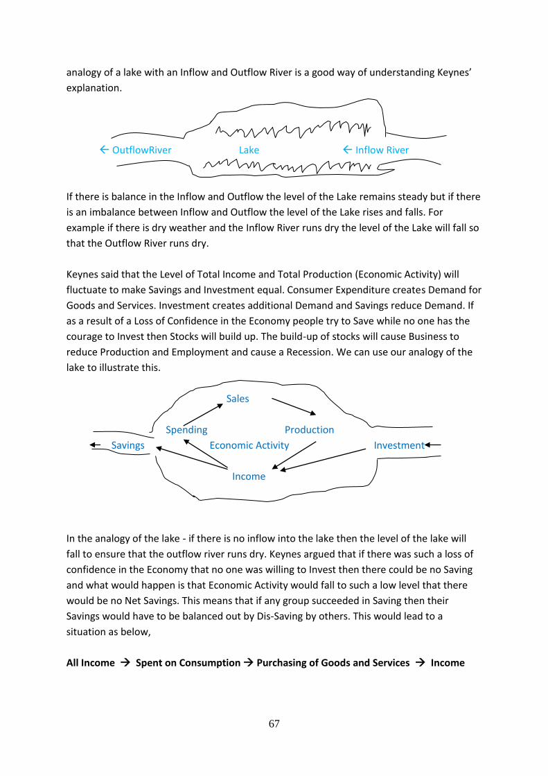
67

analogy of a lake with an Inflow and Outflow River is a good way of understanding Keynes’

explanation.

OutflowRiver Lake Inflow River

If there is balance in the Inflow and Outflow the level of the Lake remains steady but if there

is an imbalance between Inflow and Outflow the level of the Lake rises and falls. For

example if there is dry weather and the Inflow River runs dry the level of the Lake will fall so

that the Outflow River runs dry.

Keynes said that the Level of Total Income and Total Production (Economic Activity) will

fluctuate to make Savings and Investment equal. Consumer Expenditure creates Demand for

Goods and Services. Investment creates additional Demand and Savings reduce Demand. If

as a result of a Loss of Confidence in the Economy people try to Save while no one has the

courage to Invest then Stocks will build up. The build-up of stocks will cause Business to

reduce Production and Employment and cause a Recession. We can use our analogy of the

lake to illustrate this.

Sales

Spending Production

Savings Economic Activity Investment

Income

In the analogy of the lake - if there is no inflow into the lake then the level of the lake will

fall to ensure that the outflow river runs dry. Keynes argued that if there was such a loss of

confidence in the Economy that no one was willing to Invest then there could be no Saving

and what would happen is that Economic Activity would fall to such a low level that there

would be no Net Savings. This means that if any group succeeded in Saving then their

Savings would have to be balanced out by Dis-Saving by others. This would lead to a

situation as below,

All Income Spent on Consumption Purchasing of Goods and Services Income

68

But in a Modern Economy it takes a massive decline in Economic Activity to eliminate all

Savings especially as people panic and try very hard to Save as the economy goes into

recession. This is exactly what happened in the US during the early 1930s where GNP,

measured in Current Prices, fell by 46% between 1929 and 1933. During this period in the

US unemployment rose to 25% and over 10,000 banks failed.

It is easy to explain the Business Cycle using Keynesian Economics. In an Economic Boom

there is very high Demand as a result of high Investment and high Consumption. This

generates confidence and leads to high Asset Values (including Property and Shares). The

high Asset Values lead to even higher Consumer Expenditure and Investment. All this boosts

Total Demand in the economy and fuels the Boom.

When an economy goes into Recession confidence falls, Assets Values fall, Consumer

Expenditure falls and Investment falls. The decline in Total Demand drives the economy

further into Recession and the Recession feeds on itself.

Keynes advocated Demand Management by Governments to ensure that there was always

sufficient Demand to keep the level of Economic Activity High. This meant in the 1930s that

Governments should increase their own Expenditure to create Demand and Employment to

compensate for the lack of Private Sector Investment and not worry in the short-term about

balancing their Budgets. (Keynes also advocated that Government run Budget Surpluses in

Booms to prevent an Excessive level of Demand)

This was exactly what Franklin D Roosevelt, who was elected as US President in 1932, did.

Effectively Keynes created the intellectual justification for the heavy spending by the US

Government under Roosevelt’s “New Deal”.

More Complex Economy

In a Modern Economy with a Large Government Sector and International Trade the flow of

Income is more complex that in our simple example.

In this situation Total Production Y = C Sales of Consumer Goods and Services

I Sales of Investment Goods

X Export Sales

G Sales to the Government

± St Stock Changes

In this situation Total Income Y = C Purchases of Consumer Goods and

Services

S Savings

M Expenditure on Imports

T Government Taxation

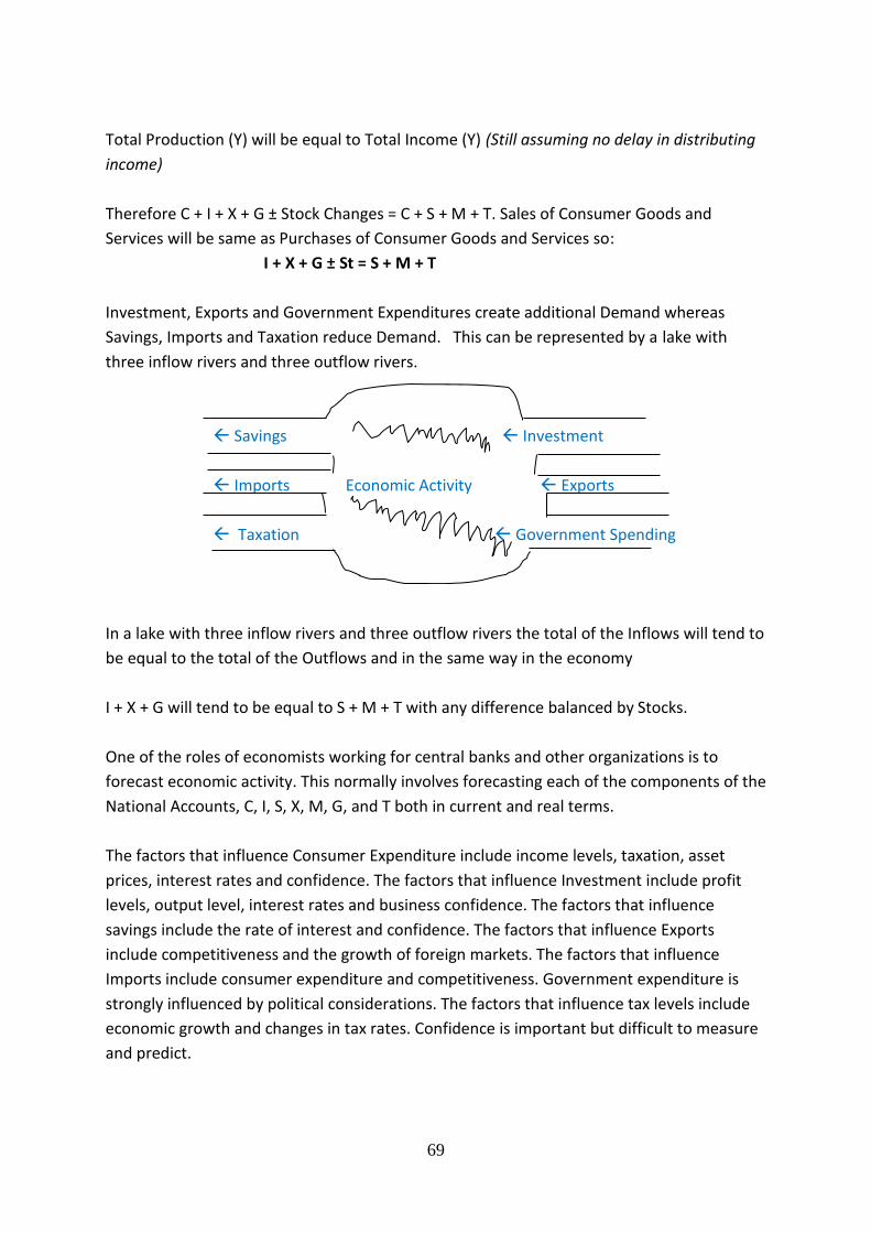
69

Total Production (Y) will be equal to Total Income (Y) (Still assuming no delay in distributing

income)

Therefore C + I + X + G ± Stock Changes = C + S + M + T. Sales of Consumer Goods and

Services will be same as Purchases of Consumer Goods and Services so:

I + X + G ± St = S + M + T

Investment, Exports and Government Expenditures create additional Demand whereas

Savings, Imports and Taxation reduce Demand. This can be represented by a lake with

three inflow rivers and three outflow rivers.

Savings Investment

Imports Economic Activity Exports

Taxation Government Spending

In a lake with three inflow rivers and three outflow rivers the total of the Inflows will tend to

be equal to the total of the Outflows and in the same way in the economy

I + X + G will tend to be equal to S + M + T with any difference balanced by Stocks.

One of the roles of economists working for central banks and other organizations is to

forecast economic activity. This normally involves forecasting each of the components of the

National Accounts, C, I, S, X, M, G, and T both in current and real terms.

The factors that influence Consumer Expenditure include income levels, taxation, asset

prices, interest rates and confidence. The factors that influence Investment include profit

levels, output level, interest rates and business confidence. The factors that influence

savings include the rate of interest and confidence. The factors that influence Exports

include competitiveness and the growth of foreign markets. The factors that influence

Imports include consumer expenditure and competitiveness. Government expenditure is

strongly influenced by political considerations. The factors that influence tax levels include

economic growth and changes in tax rates. Confidence is important but difficult to measure

and predict.

70

Case study of a Eurozone Boom

Overall Demand is made up of C + I + X +G. The Overall Demand can be appropriate, too

high or too low depending on the level of the components.

Ireland is a good example of a Country which allowed Demand to grow to an excessive level

in the run-up to the Financial Crisis. During the period 2002 to 2007 Overall Demand in

Ireland grew rapidly because of high Consumer Expenditure, high Government Expenditure

and High FDI (Foreign Direct Investment). The growth in Consumer Expenditure was driven

by rising incomes, reduced taxation, rapidly rising asset prices, low interest rates and high

general confidence. Local Investment grew rapidly because of low interest rates and high

Government Investment in Infrastructure. Government Expenditure as Tax Revenues grew

rapidly and pressure built up for better public services. This was also a period of growing US

High Tech Investment in Ireland.

A key aspect of the Irish Boom from 2002 to 2007 was a housing market bubble. The rapid

increase in house building and house prices was financed by Money Market borrowings

within the Eurozone by Irish Banks. The rising house prices created a “Wealth Effect”

consumer boom and gave a massive boost to government tax revenues. The dramatic

collapse in the Irish Housing Market in 2007/08, with the average price of houses and

apartments falling by 60%, and the World Financial Crisis led to equally dramatic falls in GNP

and Government Tax Revenues.

Keynesian Economics would have led the Irish Government to restrain expenditure, both

current and capital, during this boom. However the Government pursued a reckless policy of

spending the rapidly growing tax revenue. This meant that when the recession came in

2007/08 the Government was forced to reduce expenditure instead of increasing it. This

means that the Government inflated the boom to a disastrous level and then had to make

the recession worse by cutting expenditure.

The Financial Crisis of 2008/09 and the Great Depression in the US

During the Wall Street Crash of 1929 the authorities, the Fed and the Federal Government,

allowed a Recession to develop into “The Great Depression”. They did this by allowing over

10k banks to go bankrupt, increasing interest rates and attempting to balance the Budget.

This led to a fall of 33% in Real GDP and a rise to 25% in Unemployment.

The Financial Crisis of 2007/09 was triggered by a financial crisis in the US linked to a drop in

house prices. The reaction of the authorities in 2008 was quite different to 1929. The Fed

and the Federal Government intervened vigorously to protect the financial system to ensure

that the economic recession would not be turned into an economic collapse.

71

The Federal Reserve Bank acted to prevent the collapse of Bear Stearns, one of the World’s

leading investment bankers, in June 2007 by facilitating its takeover by JP Morgan Bank. The

Government nationalized Fannie Mae and Freddie Mac, the two largest mortgage providers

in the US in early September 2008. Fannie Mae was set up in 1938 by the FD Roosevelt

administration as part of the “New Deal” to support home ownership. US Treasury Secretary

Henry Paulson, previously Chairman and Chief Executive of Goldman Sachs, said that these

two companies were too important to be allowed to fail.

The Fed and US Government did not however intervene to protect Lehman Brothers, one of

the US’s leading Investment Bankers, who were forced to file for bankruptcy protection

under “Chapter 11” later in September 2008. The panic caused by the collapse of Lehmans

led to the takeover by Bank of America of Merrill Lynch that weekend and caused massive

problems in money markets all over the world.

The Wall Street Investment Bankers were not regulated by the Federal Reserve Bank. This

meant that they could not take deposits directly from the public or have access to the Fed

for funding but they did not have to observe Fed’s Capital Reserve Rules. By the end of

September 2008 all the big five Investment Bankers, Bear Stearns, Lehman’s, Merrill Lynch,

Goldman Sachs and Morgan Stanley had ceased to be Investment Bankers. Bear Stearns was

taken over, Lehman’s had gone bankrupt, Merrill Lynch was taken over and then Goldman

Sachs and Morgan Stanley applied to the Fed to become bankers regulated by the Fed.

The US Government also bailed out other financial institutions including AIG and Citibank.

AIG, a major insurance company specializing in financial insurance, was seen as vital to the

financial system and was given $150bn after making losses of $99bn in 2008. AIG had

insured Credit Default Swaps, effectively insurance on loans, and lost over $50bn on these.

AIG’s losses were the largest ever in US corporate history. Citibank, the world’s largest bank,

was given $45bn.

The Fed reduced interest rates from 5.25% in the summer of 2007 to 0% to 0.25% by the

end of 2008. This is the lowest rate in the history of the Fed. Holding interest rates at a

historically low rate is designed to stimulate the economy by discouraging saving and

encouraging borrowing.

The Federal Government focused on protecting the economy instead of balancing the

budget in the short-term. The incoming Obama Administration introduced a 2009 US budget

based on a €1.75 Trillion deficit equal to 12% of GDP. Much of this money was spent on

Green Energy, Infrastructure, Education and Health. The Obama Administration also put

together a support package of $275bn for the 9 million American families who were

struggling with their mortgages. All of this was on top of a $700bn rescue package for the

banks put together by the outgoing Bush Administration at the end of 2008.

72

The Obama Administration also resisted pressures towards protectionism. The Hoover

Government in 1929 introduced protectionist policies and there is always pressure for

protectionism in recessions. By resisting these pressures the US government gave a lead in

ensuring that free international trade continued during the recession.

The US reaction to the Recession of 2007/09 was exactly what Keynesian Economics would

have suggested and this prevented a complete collapse in the economy. The severity of the

Great Depression and the Great Recession can be compared by looking at the length of the

downturn, the decline in GNP, the level of unemployment and the decline in Share Prices.

In the Great Depression the downturn lasted four years with year on year declines in Real

GNP from 1929 to 1933. Real GNP fell by 33% over this period with unemployment rising

from 3% to 25%. The Dow Jones Index fell by 89% from its high in 1929 to its low in 1932.

The 2008/09 Great Recession only lasted for four Quarters recession (from summer of 2008

to spring 2009) and Real GNP fell by 4%. Unemployment rose from 4.5% to 10.0% between

February 2007 and December 2009. US unemployment started to fall in January 2010.

The fall in the Dow Jones Index from its highest in October 2007 at 14,093 to its lowest at

6,626 in March 2009 was 53%. This is disastrous and the biggest percentage decline since

the 1930s but is much better than an 89% fall. The information given above indicates that

the Great Recession of 2008/09 in the US does not compare, in terms of severity, with the

great Depression.

Dow Jones Industrial Index for 2004 to 2014.

Source, Yahoo Finance

73

The Great Recession in the PIIGS

The impact of the Great Recession was much more severe in some countries including what

are called the Eurozone “PIIGS”, Portugal, Italy, Ireland Greece and Spain. In Ireland, for

example, share prices fell by 85% including a 99% fall in bank shares, Government Tax

Revenue fell by 30%, Real GNP fell by 14%, Consumer Prices fell by 6% and Employment fell

by 17%.

The Great Recession was much more severe in the PIIGS because they all had enjoyed

massive booms before the financial crisis. These booms were fuelled by Excessive Bank

Lending and Asset Price Bubbles. This led to unsustainable growth in Government

Expenditures and loss of Competitiveness in the Private Sector. This left these economies

very vulnerable and when the Great Recession arrived they experienced an economic

collapses. The Chart below shows the Annual Change in Inflation, GNP Growth, Mortgage

Rates and Employment in Ireland since 1970.

Irish Inflation, GDP Growth, Interest Rates and Change in Employment from 1970 to 2014

Sources. All data is from the Irish Central Statistics Office, Database Direct

-15

-10

-5

0

5

10

15

20

25

70 75 80 85 90 95 0 5 10 14

Inflation

∆% in GNP

Mortgage

∆% Empl

ECBRate

74

The British Financial System

Introduction

This note covers the Financial Services Industry in London, London Money Market, the Bank

of England, the Bank of England as Government Bank, Currency Issuer, Financial Stability,

(Bankers’ Bank) and Lender of Last Resort and Monetary Policy.

London’s Financial Services Industry

London’s Financial Services industry is based in and around the “City of London”. The City of

London is one of the leading financial centres in the World. The City of London, which is a

small area in the middle of modern London, equivalent to the medieval city and often

referred to as the “square mile”, got its charter as a self-governing free city from William the

Conqueror in 1075.

The City of London’s development as a financial centre dates back to around 1300 when the

King of England, Edward 1, gave a grant of land in the city to goldsmiths and moneylenders

from Lombardy in Italy. This street is called Lombard Street.

The Royal Exchange was built as a centre for all kinds of business and trading in 1571. Over

time a variety of financial services developed in or around the Royal Exchange. Insurance

brokers established their business in Lloyd’s coffee shop around 1691. This eventually

developed into Lloyds which is the key insurance centre in the World. Lloyds, which calls

itself “the World’s specialist insurance market” had about £23 billion in premium income in

2013.

Brokers in shares were excluded from the Royal Exchange in 1698, because their shouting

distubed other traders .They transferred their business to Jonathan’s coffee shop and a

broker called Castaing started to put up a list of prices of shares and commodities in the

coffee shop. This is the origin of Stock Exchange “Listing”. The London Stock Exchange

moved into its own premises in 1801.

Britain’s dominance of World Trade in the 19th century and the strength and stability of the

British Financial System led to the emergence of London as the most important centre for

international banking and international finance in the World. (The rise of the US, as the

leading economy, and the emergence of the $, as the major reserve currency, allowed New

York to challenge London’s supremacy in the 20th century). There are now about 1,400

foreign-based financial services firms operating in London.

The London Financial Services industry has now expanded outside the City and in total

employs about 380k people. The UK’s Financial Services industry, largely based in London,

contributes about 12% of the UK government’s tax revenue.

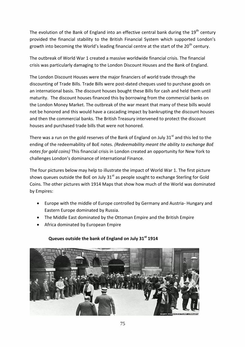
75

The evolution of the Bank of England into an effective central bank during the 19th century

provided the financial stability to the British Financial System which supported London’s

growth into becoming the World’s leading financial centre at the start of the 20th century.

The outbreak of World War 1 created a massive worldwide financial crisis. The financial

crisis was particularly damaging to the London Discount Houses and the Bank of England.

The London Discount Houses were the major financiers of world trade through the

discounting of Trade Bills. Trade Bills were post-dated cheques used to purchase goods on

an international basis. The discount houses bought these Bills for cash and held them until

maturity. The discount houses financed this by borrowing from the commercial banks on

the London Money Market. The outbreak of the war meant that many of these bills would

not be honored and this would have a cascading impact by bankrupting the discount houses

and then the commercial banks. The British Treasury intervened to protect the discount

houses and purchased trade bills that were not honored.

There was a run on the gold reserves of the Bank of England on July 31st and this led to the

ending of the redeemability of BoE notes. (Redeemability meant the ability to exchange BoE

notes for gold coins) This financial crisis in London created an opportunity for New York to

challenges London’s dominance of international Finance.

The four pictures below may help to illustrate the impact of World War 1. The first picture

shows queues outside the BoE on July 31st as people sought to exchange Sterling for Gold

Coins. The other pictures with 1914 Maps that show how much of the World was dominated

by Empires:

Europe with the middle of Europe controlled by Germany and Austria- Hungary and

Eastern Europe dominated by Russia.

The Middle East dominated by the Ottoman Empire and the British Empire

Africa dominated by European Empire

Queues outside the bank of England on July 31st 1914

76

Europe in 1914 The Middle East in 1914 Africa in 1914

London Money Market The London

Money Market is a market in short-term loans based in London. The period of the loans can

be from overnight to 1 year. The Rate of Interest in the London Money Market is called the

Libor Rate. Libor (or LIBOR) stands for London Interbank Offered Rate. The Libor Rate is

important in that it is widely used as a benchmark for determining the rate of interest on

loans all over the world.

A Libor rate is established each day in London for 5 different currencies and for 8 different

time periods. These currencies are £, $, €, Swiss Franc (CHF) and Japanese Yen.

The London Money Market originated in the early 19th century with the growth in the use of

Bills of Exchange to finance trade. Bills of Exchange were effectively post-dated cheques

guaranteed by a bank (Underwritten), that purchasers of goods used to pay for the goods.

When the seller of goods received a Bill of Exchange s/he would often require cash before

the maturity date of the cheque. Certain businesses specialized in the purchasing of Bills of

Exchange and they became known as Discount Houses.

The Discount Houses purchased Bills at a discount on face value and held the Bills until

maturity. For example if the owner of a Bill of Exchange worth BD100, but with a maturity

date in six months, needed cash then s/he could sell the Bill to a Discount House. If the

Discount House paid BD96 for the Bill they would have invested BD96 for 6 months in the

hope of getting BD100 in 6 months making a return on Investment of over 8% per annum.

During the 20th century the use of Bills of Exchange was reduced but this was balanced by

the growth of Commercial Bills and Treasury Bills. The Discount Houses are the major

purchasers of UK Treasury Bills. The Discount Houses either hold Treasury Bills to maturity

or sell them to other financial institutions.

Discount Houses finance their businesses by borrowing short-term from commercial banks.

The Bank of England found the role of the Discount Houses so useful that it rescued them in

1914 at the outbreak of World War 1 when many Bills of Exchange became worthless. The

77

BoE counts loans by commercial banks to the Discount Houses (“Call Money”) as Reserve

Assets.

Origins of the Bank of England

The basic model for Central Banking is the Bank of England, the Central Bank of the UK. The

Bank of England (BoE) developed central banking gradually over its long history and the

history of the BoE gives some insight into the nature of central banking. The role of a Central

Bank is normally seen as:

Acting as the Government’s Bank

Issuing the currency of the State or Group of States

Acting as Bankers’ Bank(Financial Stability Policy)

Managing Interest Rates (Monetary Policy)

Managing the Foreign Exchange Rate (Exchange Rate Policy)

This note will cover the first four roles and the discussion of Exchange Rates will follow in

Section 10.

In 1688 William of Orange, from Holland replaced his father-in-law, James II as King of

England, Scotland, Wales and Ireland. The civil war that followed lasted until the defeat of

James in Ireland in 1690. This was followed by a war with France. The Government of

William was heavily in debt and a group of businessmen, including many of the people who

organised the overthrow of James and his replacement by William, saw an opportunity to

get involved in the business of banking.

In 1694 this group of businessmen offered the government, who were then in Bagehot's

words “in desperate want of money”, a loan of £1.2 million, at the very high interest rate of

8% per annum, in exchange for a Royal Charter for a bank, with important privileges, to be

known as the Bank of England.

The introduction to the act describes it as “An Act for granting to theire Majesties severall

Rates and Duties upon Tunnage of Shipps and Vessells and upon Beere Ale and other Liquors

for secureing certaine Recompenses and Advantages in the said Act mentioned to such

Persons as shall voluntarily advance the summe of Fifteene hundred thousand pounds

towards the carrying on the Warr against France”.

The BoE was the only Joint Stock bank allowed to issue banknotes in England and Wales. By

joint stock is meant that the BoE could have many shareholders and so had access to a large

capital base. This large capital base, the high income from the government loan and the

powerful connections of the major shareholders made the BoE a powerful organization

from the very beginning.

78

The 1694 act prevented the bank from engaging in any activities other than issuing and

trading in “bills”, coins and bullion. This was because the persons who contributed the

original capital were businessmen. These businessmen did not want the bank to use its

great power to compete with them in their own business activities.

The Bank of England as Government Bank

From its foundation the BoE acted as the government bank in Britain and managed the

national debt. Its role as Government bank helped the BoE to become the dominant bank in

England and Wales. When Henry Thornton wrote about the role of the BoE in 1802 he even

described it as “The National Bank”. Walter Bagehot wrote in 1873 about “the popular

conviction that the Government is close behind the Bank, and will help it when wanted.

Neither the Bank nor the Banking Department have ever had an idea of being put 'into

liquidation;' most men would think as soon of 'winding up' the English nation.”

The bank, however, during most of its history remained in an ambiguous position. Its close

relationship with the Government meant that it was often seen as a “National Bank” which

required it to act in the national interest. However it was a private bank and was owned and

controlled by its shareholders. These shareholders required it to act in their interest and

generate as much profit as possible for its owners. These tensions continued to exist until its

role as a National Bank or Central Bank became almost universally accepted by the end of

the 19th century.

The BoE remained a private business for 250 years and was only nationalized in 1946. The

fact that it was a private business during most of its history was crucial in ensuring that it

had a degree of independence from government.

Currency Issue

The Bank of England’s notes, which are referred to in UK legislation as “promissory notes of

the governor and company of the Bank of England, payable on demand” became in the

BoE’s own word’s “a widely accepted currency as people seldom doubted that the “promise

to pay” which referred to gold coin of the realm would be honored”.

The bank used to purchase gold “bullion” at £4 per ounce and mint it into coins. The original

gold coins minted by the BoE held exactly ¼ ounce (120 grains) of pure gold. The BoE always

redeemed their banknotes with these gold coins at the rate of one gold coin for a pound. In

1797 during a war with France, there was a run on the bank and the “redeemability” of the

bank’s notes had to be suspended.

Thornton showed that the confidence in the BoE notes was so high that the loss of

redeemability in 1797 did not affect the acceptance of BoE notes as payment.

Redeemability was re-established in 1821 and lasted until 1914. When redeemability of the

£ was re-established in 1821 the weight of the new gold coins being minted was 113 grains

79

of gold and the pound was redeemable in terms of one gold coin per £. The bank’s notes

were made Legal Tender in 1833, even though the bank was a private business, which

meant that they had to be accepted for payment of debts.

Redeemability of Sterling in gold ended at the start of World War 1, as explained above, and

was never reestablished.

Financial Stability, (Bankers’ Bank and Lender of Last)

The BoE’s role as Bankers’ Bank evolved naturally during the 18th and 19th century. The

prestige and power of the Bank of England led to a situation where most other banks kept

an account with the Bank of England and kept their surplus deposits with the bank. Most

other banks were therefore customers of the BoE and if they needed money they borrowed

from the BoE in the normal course of business.

The Bank’s role as “Lender of Last Resort” evolved from its normal lending activities to

banks. During bank panics some banks would find it impossible to borrow from other banks

and so were forced to borrow from the BoE. The bank developed its approach as “Lender of

Last Resort” based on practical experience in handling financial crises. The bank learned

both from its successes and its failures. A theoretical understanding of the role of the BoE as

Lender of Last resort was developed in the writings of bankers and economists such as

Henry Thornton (writing in 1802) and Walter Bagehot ( writing in 1873).

Britain was the first country in the world to develop large-scale deposit banking. With

deposit banking there is always a risk of financial instability in that most deposits can be

withdrawn immediately yet to make a profit the bank must lend for a long period. Banks

have to manage their lending risks against the need for liquidity. This led to regular financial

crises from the end of the 18th century. These financial panics required intervention by

either the BoE or the British Treasury to protect the banking system.

Thornton showed that the BoE failed to stem a financial crisis in 1793 when it refused to

issue more notes against good security and the British Treasury had to solve the problem by

issuing Exchequer Bills against good security.

Henry Thornton, who is sometimes referred to as the “father of Central Banking” advocated

that the BoE be less timid in future and not worry about the impact of the extra cash that

banks demanded in financial crisis on inflation. Thornton argued that the circulation of

money slows during times of financial stress as hoarding creates a shortage of cash.

The BoE did behave with courage in a major financial panic in 1825. Harman, the Governor

of the Bank of England, describing how the bank managed the panic said “We lent it by

every possible means and in modes we had never adopted before; we took in stock on

security, we purchased Exchequer bills, we made advances on Exchequer bills, we not only

discounted outright, but we made advances on the deposit of bills of exchange to an

80

immense amount, in short, by every possible means consistent with the safety of the Bank,

and we were not on some occasions over-nice. Seeing the dreadful state in which the public

were, we rendered every assistance in our power. After a day or two of this treatment, the

entire panic subsided, and the 'City' was quite calm”. (Quote from Bagehot’s “Lombard

Street”.)

Walter Bagehot in his Essay “Lombard Street”, published in 1873, showed how important

the British financial system was to the success of Britain as the world’s dominant economic

and trading power and the key role that the BoE played in the system.

Bagehot wrote that “The directors of the Bank are, therefore, in fact, if not in name, trustees

for the public, to keep a banking reserve on their behalf; and it would naturally be expected

either that they distinctly recognized this duty and engaged to perform it, or that their own

self-interest was so strong in the matter that no engagement was needed. But so far from

there being a distinct undertaking on the part of the Bank directors to perform this duty,

many of them would scarcely acknowledge it, and some altogether deny it”.

Bagehot explained the ambiguity in the role of the BoE as a private bank but having a

national interest. “It might be expected, he wrote, that as this great public duty was cast

upon the Banking Department of the Bank, the principal statesmen (if not Parliament itself)

would have enjoined on them to perform it. But no distinct resolution of Parliament has ever

enjoined it; scarcely any stray word of any influential statesman.”

Bagehot noting the reluctance of both the Bank of England, and the government, to

acknowledge this “great public duty” concluded “as we have seen, though the Bank, more or

less, does its duty, it does not distinctly acknowledge that it is its duty”

Carrying out “this great public duty” of protecting the British financial system required in

Bagehot’s words “In opposition to what might be at first sight supposed, the best way for

the bank or banks who have the custody of the bank reserve to deal with a drain arising from

internal discredit, is to lend freely.”

He also worked out the principles of Central Banking showing how the Bank of England

could protect the stability of this financial system, “an immense system of credit, founded on

the Bank of England as its pivot and its basis, now exists. The English people, and foreigners

too, trust it implicitly in effect”.

The effective working of the Bank of England required in his view:

“First. There should be a clear understanding between the Bank and the public that, since

the Bank hold out ultimate banking reserve, they will recognise and act on the obligations

which this implies; that they will replenish it in times of foreign demand as fully, and lend it

in times of internal panic as freely and readily, as plain principles of banking require.”

81

“Secondly. The government of the Bank should be improved in a manner to be explained. We

should diminish the 'amateur' element; we should augment the trained banking element;

and we should ensure more constancy in the administration.”

“Thirdly. As these two suggestions are designed to make the Bank as strong as possible, we

should look at the rest of our banking system, and try to reduce the demands on the Bank as

much as we can. The central machinery being inevitably frail, we should carefully and as

much as possible diminish the strain upon it.”

The policies pursued by the BoE gave Britain a 150 year period of financial stability. If a bank

got into financial difficulty the BoE sorted the issue out without the general public becoming

aware of the problem so that no panic occurred. If the issue was one of liquidity then the

BoE provided the necessary liquidity. If the issue was one of solvency then the BoE arranged

a take-over of the bank.

One hundred and fifty years of financial stability led to a widespread belief in Britain that

financial instability and bank runs were merely historical events. This created the

environment for the disastrous “reforms” under the 1998 Bank of England Act.

The 1998 “reforms” gave autonomy to the Bank of England in Monetary Policy but also set

up an Independent Financial Services Authority (FSA) to control the individual banks. This

meant that the BoE was in charge of interest rates but the FSA was in charge of bank

regulation. This act also required the BoE to disclose any lending to banks. This system broke

down during the financial crisis of 2007/08 as confusion developed as to who should take

the lead in dealing with a crisis in Northern Rock Bank. Worse still, the BoE was forced to

disclose that it had lent money to Northern Rock. This led to a panic and a run on the bank.

Northern Rock had specialized in providing long term loans for housing and financed this by

borrowing on the money market. As the sub-prime crisis developed in the US, the money

market loans dried up for Northern Rock. On September 14th 2007 the BoE had to provide a

loan of £25 billion and a guarantee of a further £30 billion to allow the bank to survive. The

run on the Northern Bank was provoked by a BBC report on September 13th by Robert

Peston, BBC Financial Correspondent, that Northern Bank had sought assistance from the

BoE. The run on the Northern Bank was covered by a Channel 4 TV Program on September

17th 2007

Northern Rock shareholders were wiped out and eventually the bank was sold to Virgin and

now operates as Virgin Bank but most of the BoE loans have been repaid.

In total the BoE or the UK Treasury had to provide £850 billion in shares, loans and loan

guarantees to banks and insurance companies during the crisis although most of this has

been or will be repaid.

82

The experiment with breaking up the Bank of England and handing some of its role to the

FSA was a disaster. The FSA was re-integrated into the BoE in 2009.

The role of the FSA is now played by an office within the BoE called the Prudential

Regulatory Authority (PRA) which was set up in 2012. In 2013 the PRA started stress-testing

the 8 largest UK banks using the Basel 3 Guidelines. The banks were RBS, Barclays, HSBC,

Bank Santander UK, Lloyds, Standard Chartered, The Cooperative Bank and Nationwide. The

BoE wanted each bank to have a Basel 3 Capital Ratio of above 7% of Risk Weighted Assets.

Five of the 8 banks failed the test based on their 2012 accounts and had to either raise

capital or reduce their assets.

Stress testing has continued on an annual basis. The 2014 stress tests which covered the top

7 banks (Nationwide not included) assumed, among other things, a 35% fall in UK house

prices. The Cooperative Bank failed the 2014 stress test and was forced to raise finance and

reduce their balance sheet. Barclays had a bare pass and they were forced to forego a

payment of dividends to shareholders. The 2015 stress tests will be confined to the top 6

banks as Nationwide and The Cooperative Bank are not included. The 2015 stress tests

assume, among other things, a 20% fall in UK house prices and a 40% fall in Hong Kong

house prices.

Monetary Policy

Monetary Policy, which involves influencing the level of economic activity though variations

in the short term rate of interest, only became an important activity in the 1980s. Between

1945 and 1976 the consensus was that the correct way to control overall economic activity

was through “Fiscal Policy”. Fiscal Policy works through varying the overall government

budget surplus or deficit by changing expenditure and taxation.

The Bank of England was nationalized in 1946 and it lost its independence. The UK Treasury

decided what the rate of interest should be and it was the job of the BoE to implement the

Treasury policy.

The economic policies pursued between 1945 and 1976 led to a massive expansion in the

role of the state in the economy and to growing inflation. The led to what is often referred

to as “Stagflation” which was economic stagnation combined with inflation. Economic

stagnation, inflation, excessive power of the trade unions and rising national debt forced the

British government to apply for a bailout from the International Monetary Fund in 1976.

This was followed by 3 years of economic and political instability until Margaret Thatcher

was elected as British Prime Minister in 1979.

Thatcher’s government pursued what were called “Monetarist Policies” which involved the

government balancing its budget and controlling inflation through controlling the Money

Supply. During this period the BoE tried to ensure that the Money Supply was controlled by

forcing up interest rates. A combination of cuts in government expenditure to balance the

83

budget and high interest rates to combat inflation led to a severe economic recession at the

start of the 1980s. These policies were similar to those being pursued in the US at the same

time.

In 1979 the European Union decided to start moving towards a single currency, by linking

currency exchange rates in what was called the European Monetary System (EMS). Britain

decided not to become involved in the setting up of the EMS. Britain joined the EMS in 1990

but was forced out of the system and forced to devalue sterling by massive foreign

exchange speculation against the currency in September 1992. Since 1992 the £stg has been

allowed to float on the foreign exchange market with its value determined by the market.

The EMS developed into the Euro but Britain remains outside the Eurozone.

The BoE was given full control of Interest Rates and Monetary Policy by the Labour

Government in 1997 and this was confirmed by the 1998 Bank of England Act. The Bank

says that its role is “Promoting the good of the people of the United Kingdom by maintaining

monetary and financial stability”.

The 1998 Act directed the BoE, as its top priority, to pursue monetary policies to achieve

“price stability” which is defined as an inflation rate of 2% pa. The policy is implemented by

the Monetary Policy Committee, (MPC) of the BoE which normally meets once per month to

set interest rates.

The Governor of the BoE is required to write a letter to the Chancellor of the Exchequer if

the rate of inflation is more than 1% away from the target. The MPC is also required to

target economic growth and full employment.

The BoE has been making short term loans available to banks since 1694. The rate of

interest on these loans has been called by a variety of names in that period. From 1694 until

1972 the rate was called the Bank Rate, from 1972 to 1996 it was called the Minimum

Lending Rate, from 1996 to 2006 it was called the Repo Rate (Repurchase Agreement Rate)

and since 2006 it is called the Official Bank Rate.

Between 1694 and 1914 the rate moved between 2% and 10% but most of the time it was

around 3 to 4%. It was only during a period of acute financial instability that the rate was

increased above 5%. For example in 1914 the BoE increased its rate to 10% as WW1

commenced. During the Great Depression the rate never went below 3% and for some time

it was at 6%.

During the Financial Crisis in 1976 which led to borrowing from the IMF the rate went to

17% and it remained very high for the next ten years as Britain experienced high inflation

and as the Thatcher Government used high interest rates to combat this inflation.

84

In 2003 the Official Bank Rate was 3% and then as the economy recovered the rate was

increased to 5.75% in 2007. The financial crisis led to a rapid cut to 0.5% in 2009 and it has

remained at 0.5% for the last 5 years. The simplified chart below only shows the Bank of

England’s Official Bank Rate at end of June each year.

Source BoE Official Bank Rate

The Bank has kept its Official Bank Rate at 0.5% from 2009 until April 2015 to encourage a

recovery in the UK economy and push up inflation to 2% after the Great Recession but this

recovery, as shown in the next graph, was very slow at happening and the inflation rate is

now (April 2015) 0.0% pa compared with a target of 2.0%pa.

UK GDP Growth and Inflation from 2005 to 2014

Source, Office for National Statistics

0

5

10

15

20

80 85 90 95 0 5 10 15

Bank of England Official Bank Rate

BoE Rate %

-8

-6

-4

-2

0

2

4

6

0 1 2 13 4 5 6 7 8 9 10 11 12 13 14 15

GDP Growth

Inflation

BoE given

control of

Monetary

Policy in 1997

85

Quantitative Easing As

the cut in the Official Bank Rate to 0.5% did not lead to immediate economic recovery the

BoE decided in January 2009 to start a policy of Long Term Asset Purchase which is referred

to as Quantitative Easing (QE).

This policy was following the lead of the US Federal Reserve Bank which started QE in

November 2008. QE was designed to force down long term interest rates to aid economic

recovery. Under its QE policy the BoE purchased Long-term Securities – over 99% UK

Government Securities. Under QE the BoE purchased £375 billion of assets. This had the

effect of forcing up security prices and forcing down long term interest rates.

Low interest rates normally lead to high asset prices including property prices. During 2013

and 2014 UK property prices, especially house prices, started rising rapidly and the BoE

became concerned that this could lead to another housing bubble. In June 2014 the bank

introduced restrictions on lending to the housing market. These restrictions controlled the

amount of the loan relative to the income of the borrower and introduced stress tests to

ensure that borrowers would be able to service the loans after a 3% increase in rates.

The UK economy started growing at about 3% in 2014. In Q4 2014 GDP was estimated to

have been 4% higher than the pre-economic downturn peak of Q1 2008. From the peak in

Q1 2008 to the trough in Q2 2009, the economy shrank by 6.0%. This decline has now been

fully recovered and the excellent growth rate is leading to speculation that the BoE will

increase the Official Interest Rate during 2015.

Forward Guidance

Forward Guidance is now one of the policy instruments of the BoE’s Monetary Policy.

Forward Guidance involves the BoE, or any other central bank, giving clear information on

how it sees short term interest rates developing in the near future as a way of guiding

market expectations about changes in interest rates.

Forward Guidance was first used by the BoE in August 2013. The Monetary Policy

Committee (MPC) said it would leave interest rates unchanged at 0.5% at least until the

unemployment rate had fallen to 7%, provided there weren’t risks to inflation or financial

stability.

By February 2014, unemployment had fallen close to 7%. The MPC said there remained

room for growth in the economy before raising interest rates. The MPC also promised that

increases in interest rates will be gradual and limited. This statement has been

supplemented by a BoE assessment of its own Monetary Policy during the Great Recession

and how it sees Monetary Policy developing as the economy recovers.

The Diagram below shows the sequence of Bank of England Monetary Policy actions

designed to stimulate economic recovery.

86

Source, UK Office of National Statistics

The British Pound and the Euro

During the period when the Euro was being planned and developed Britain was ambiguous

about joining a Common European Currency. The other European countries agreed a system

of fixed exchange rates for their currencies, as predecessor to a European currency in 1979.

Britain did not join this fixed exchange rate system at the beginning but did join in 1990.

However Britain was forced out of the fixed exchange rate system by massive speculation

against the currency in September 1992.

The European Monetary System developed into the Euro, which became the common

currency of most European Union countries and was launched in 2002. Britain has remained

outside the Euro. This has been a great advantage to Britain during the Financial Crisis of

2008 and the Great Recession as it allowed the bank of England to retain full control of the

UK financial system and pursue Monetary Policies suited to the needs of the UK economy.

London, as one of the World’s greatest financial centres, would almost certainly have been

the headquarters for the European Central Bank. When Britain pulled out of the planning for

the Euro it led to the ECB being located in Frankfurt. Another disadvantage to the retention

of the Pound is that the value of the Pound fluctuates relative to the Euro and this

complicates trading with the majority of EU countries. This is illustrated by the screenshot

below from Yahoo Finance which shows the Euro to Sterling Exchange Rate for the last 5

years.

-8

-6

-4

-2

0

2

4

6

8

0 1 2 13 4 5 6 7 8 9 10 11 12 13 14 15

GDP Growth

Inflation

Bank Rate Bank

Rate

Q

E

Forward

Guidance

87

References Walter Bagehot,

Editor of the Economist Magazine, 1873, Lombard Street, a description of the Money

Market. Henry Thornton, London

Merchant Banker, 1802, An Enquiry into the nature and effects of the Paper Credit of Great

Britain. The-great-northern-rock-

bank-run

Minutes of Monetary Policy Committee

http://www.bankofengland.co.uk/publications/minutes/Documents/mpc/pdf/2014/mpc14

08.pdf

88

The US Financial System

Introduction

This note covers the New York Financial Services Industry, the First and Second Banks of the

US, the National Banks, the Federal Reserve Bank, Financial Stability Policy, Monetary Policy,

Taylor Rule, “Quantitative Easing”, “Forward Guidance”, Inflation Targets and Economic

Recovery in the US.

New York Financial Services Industry

The US had over 5,600 commercial banks at end of 2014. This number is down from over

14k in the 1980s. US banks hold over $14trillion in deposits. The US banking industry is

centred on New York.

The Financial Services industry started in New York with the setting up of the Bank of New

York in 1784. In 1792 the First Bank of the United States, see below, opened a branch in NY

and the New York Stock Exchange (NYSE) was established in 1792 and traded in the Tontine

Coffee Shop from 1793.

New York became the leading financial services centre in the world, displacing London, after

World War 1. This was linked to the emergence of the US as the World’s leading economy

and the decision of the US in 1914 to maintain the redeemability of the $ in terms of gold.

There are about 350k persons working in Financial Services in New York. The two leading

stock exchanges in the world in terms of Market Capitalization are the New York Stock

Exchange (NYSE) and Nasdaq. Before the financial crisis in 2008 the 5 top banks in the

World, based on revenue, had their head offices in New York.

New York’s dominance of Financial Services is being eroded with the rise of stock markets in Europe and Asia and the renewal of London’s dynamism in international financial services. London is seen as more attractive than NY in terms of regulation particularly in the cost and

simplicity of regulation. (An example of the complexity of US regulation is that the Volker

Rule, part of the Dodd-Frank Act Consumer Protection Act of 2010 runs to almost 1100

pages).An example of the complexity of US regulation is that the Volker Rule, part of the

Dodd-F rank Act Consumer Protection Act of 2010 runs to almost 1100 pages . London has

emerged as the major world centre for derivative trading.

The First and Second Banks of the US

The US has two forms of banks, state banks and federal banks. At the foundation of the US

all banks were chartered by their state but their business was confined to that state.

89

After the US won its independence from Great Britain in 1776 there was a desire among

many business people and politicians to set up a National Bank that could operate all over

the US and could perform a role similar to the Bank of England. There was also opposition to

a strong national bank from groups such as farmers who disliked bankers. The First Bank of

the United States was given a charter by the Federal Government in 1791 but this was only a

20 year charter and the charter was not renewed in 1811.

In 1812 the US got involved in a war with Great Britain. In 1813 the British captured

Washington and burned the White House. During the war the US Government realized that

they needed a large powerful bank to raise finance for the war by selling government bonds.

This eventually led to the setting up of a second national bank.

The Second Bank of the United States was given a 20 year charter in 1816 but in 1836 its

charter was also not renewed. This meant that America only had small state-chartered

banks which only operated within their own state. This created many difficulties including

very poor quality bank notes and problems for the government in raising finance.

During the US Civil War, which lasted from 1861 to 1865, the “Union” government, with

Abraham Lincoln as President, could not raise enough funding and the US Treasury started

printing “United States Notes”. These were “legal tender” and were used to help finance the

war although the government had other sources also including tax revenues and war bonds.

National Banks

In 1863 the National Banking Act was passed by Congress. This act provided for the setting

up of banks with national charters that could carry on banking all over the US. The act also

led to the ending of note issue by the state banks. The national banks had to follow rules on

Capital and Reserves. The national banks could only issue banknotes if they were fully

backed by US government securities.

Even after the setting up of the national banks there was no agency that could lend notes to

commercial banks, secured by bank assets, during a financial panic. There were regular

financial panics in the US over the following 40 years. These included panics in 1873, 1884,

1890, 1893 and 1907. These financial panics led to bank collapses, losses by depositors and

“Trade Recessions”.

The 1907 financial crisis led to a large number of bank failures and would have been much

worse only for the actions of JP Morgan who coordinated the major banks in New York to

provide funding for other banks.

A consensus emerged after 1907 that the US needed a Central Bank but there was no

consensus on who should control the new bank or how it should be organized. The larger

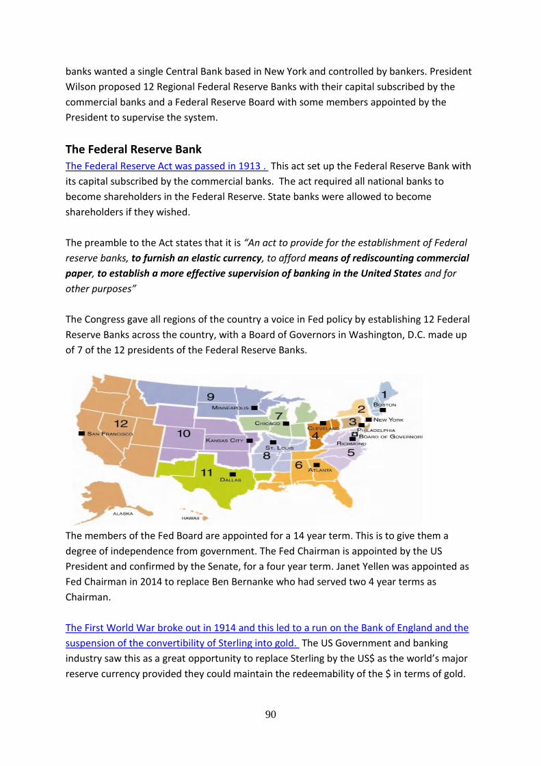
90

banks wanted a single Central Bank based in New York and controlled by bankers. President

Wilson proposed 12 Regional Federal Reserve Banks with their capital subscribed by the

commercial banks and a Federal Reserve Board with some members appointed by the

President to supervise the system.

The Federal Reserve Bank

The Federal Reserve Act was passed in 1913 . This act set up the Federal Reserve Bank with

its capital subscribed by the commercial banks. The act required all national banks to

become shareholders in the Federal Reserve. State banks were allowed to become

shareholders if they wished.

The preamble to the Act states that it is “An act to provide for the establishment of Federal

reserve banks, to furnish an elastic currency, to afford means of rediscounting commercial

paper, to establish a more effective supervision of banking in the United States and for

other purposes”

The Congress gave all regions of the country a voice in Fed policy by establishing 12 Federal

Reserve Banks across the country, with a Board of Governors in Washington, D.C. made up

of 7 of the 12 presidents of the Federal Reserve Banks.

The members of the Fed Board are appointed for a 14 year term. This is to give them a

degree of independence from government. The Fed Chairman is appointed by the US

President and confirmed by the Senate, for a four year term. Janet Yellen was appointed as

Fed Chairman in 2014 to replace Ben Bernanke who had served two 4 year terms as

Chairman.

The First World War broke out in 1914 and this led to a run on the Bank of England and the

suspension of the convertibility of Sterling into gold. The US Government and banking

industry saw this as a great opportunity to replace Sterling by the US$ as the world’s major

reserve currency provided they could maintain the redeemability of the $ in terms of gold.

91

The US Government decided that they would maintain the convertibility of the $ into Gold.

Foreign Investors had invested heavily in US business, particularly in the railways. The

Government closed the NYSE for 4 months from July 31 to make it difficult for foreign

countries to sell their US investments. If countries could sell their US investments they

would be paid in $s which they would then want to convert into gold. This would have

created a drain on US gold reserves. In addition the US would only export in exchange for $s

or gold and this created a demand for $s which also protected the gold reserves. The US

Treasury also provided emergency loans to banks. The emergency loans to banks prevented

financial panic.

The Fed was established in November 1914. The first major test of the Fed after 1914 was in

1929 with the start of the “Great Depression”. The failure of the Fed in 1929 is in sharp

contrast with the success of the US Treasury in 1914.

The Fed responded inadequately to bank runs and bank failures that swept the US. More

than 10,700 of the nation's 25,000 banks (at the end of 1928) suspended operations

between 1929 and 1934.

Bank depositors suffered significant losses in bank failures - on average about 20% of the

value of the deposits. In 1934 the US introduced bank deposit insurance by setting up the

FDIC, Federal Deposit Insurance Corporation under the FDIC Act of 1933.

Between World War II, which ended in 1945, and the recent financial crisis, macroeconomic

stability was the predominant concern of most central banks including the Fed as there was

general financial stability.

From 1950 to 1973 the Fed sought to keep both inflation and economic growth reasonably

stable but gave priority to economic growth. Inflation gradually increased and then the oil

price increases of 1973 and 1978 pushed the inflation rate even higher. This is shown in

the next chart which shows US annual inflation rates since 1930.

-15

-10

-5

0

5

10

15

20

30 40 50 60 70 80 90 0 10

% C

han

ge

US Annual Inflation, 1930 - 2014

Inflation

92

The increase in oil prices in the 1970s and the increases in wages that it triggered led to a

surge in inflation and inflation expectations. Inflation reached almost 15% per year in the

late 1970s, see Chart 1 above, and controlling inflation became a political, economic and

financial priority. Fed Chairman Paul Volcker (1979 – 1987) announced, in October 1979, a

dramatic break in the way that monetary policy would operate.

The new approach to monetary policy, adopted by Paul Volker, involved controlling inflation

through controlling the Money Supply. In practice this involved very high interest rates (in

June 1981 the Federal Funds Rate reached a peak at 20%) to reduce demand and bring

down growth - effectively generating unemployment. The Fed policy of reducing the

inflation rate through high interest rates forced up interest rates worldwide and caused a

severe worldwide recession in 1981 and 1982.

In the recession at the start of the 1980s, US Real GDP fell by 2% in 1982 and unemployment

peaked at nearly 11% in 1983.

Chart 2

The US economy experienced a combination of stagnation and inflation in the early 1980s.

This is shown clearly in the next graph which shows GDP Growth and Inflation. The

combination of stagnation and inflation was called Stagflation.

-15

-10

-5

0

5

10

15

20

25

30 40 50 60 70 80 90 0 10

% C

han

ge

US Annual GDP% Growth

GDP%

Volker

Recession

WW2

39-45

Financial

Crisis

Great

Depression

93

Chart 3

From the 1987 to 2007 (Fed Chairman - Alan Greenspan), GDP grew steadily with low

inflation and only a small recession in 1992. This period is often called "The Great

Moderation." Because of the Financial Stability during this period, monetary policy received

greater emphasis than financial stability policies. Most financiers and economists believed

that financial stability was assured and that bank runs and bank collapses were just part of

history and not possible in the modern US financial system.

Financial Stability Policy

Financial Stability Policy is about ensuring the stability of the financial system. This role of a

central bank is often referred to as acting as banker’s bank. During the twenty years up to

2007 there was a growing tendency to take financial stability for granted in the US. This

overconfidence allowed actions and practices to develop which threated the stability of the

US financial system.

These actions and practices included:

Repeal of the Glass - Steagal Act

Excessive lending for property

Development of new complex Financial Instruments

Increased importance of unregulated banks

The (Glass - Steagal Act) US Banking Act of 1933 was introduced to reduce the risk of bank

failures by imposing restrictions on the activities of commercial banks. Banks were not

allowed to get involved in complex securities trading. In effect Glass - Steagal separated

normal banking activities such as accepting deposits, giving loans etc from investment

banking. During the 1990s pressure built up to eliminate these restrictions and the GLBA

-15

-10

-5

0

5

10

15

20

-15

-10

-5

0

5

10

15

20

25

30 40 50 60 70 80 90 0 10

% C

han

ge

US Annual GDP% Growth and Inflation, 1930 - 2015

GDP%

Inflation

Stagflation

94

Act of 1999 repealed Glass - Seagal and allowed banks to get involved in securities trading

and other high risk financial activities.

One of the key reasons for the financial crisis of 2008 was the excessive lending to property.

Prior to the early 2000s, US homebuyers typically made a significant down payment and

lenders were very careful about accurate documentation. The Fed's low interest rate

monetary policy in the early 2000s made house purchase very attractive and led to rising

prices.

Rising house prices created an expectation that housing was a "can't lose" investment. A

surge in Sub-Prime Lending (Loans to borrowers with high risk) and ARMs, Adjustable Rate

Mortgages , drove up demand for housing, raising prices further.

Complex Financial Instruments were developed with very little regulation or understanding

of the risks involved. One of category of such instruments was securitization of home loans.

Lenders “bundled” home loans into Mortgage Backed Securities which they sold as low risk

investments and then used the money they raised to give further house loans. Fannie Mae

and Freddie Mac are two US Government-backed Agencies that helped to finance home

purchases by purchasing these Mortgage Backed Securities (MBS). They funded their MBS

purchases through short-term borrowings on the Money Market.

US House Prices more than doubled between 2000 and 2006 as shown by the Case – Schiller

Index of House Prices below. Rising House Prices combined with rising interest rates

eventually led to a drop in demand for houses. Declining demand for houses led to a drop in

house prices beginning in early 2006.

US House prices fell by about 40 percent between 2006 and 2008. Many house owners,

particularly Sub-Prime ARMs Borrowers had “Negative Equity” and could not meet

payments. Mortgage delinquencies and foreclosures surged. The number of houses for sale

grew rapidly and prices fell. Banks and other holders of Mortgage Backed Securities suffered

sizable losses—a key trigger of the crisis.

Case – Schiller Index of US House Prices from 2000 to 2014

95

Source Case Schiller

As investors realized that the housing market was collapsing they withdrew funding from all

organisations linked to housing finance including Fannie Mae and Freddie Mac. These two

companies were rescued by the US Treasury which guaranteed loans of $200 billion to each

of them.

Many of the Mortgage Backed Securities were insured by AIG, the largest Insurance

Company in the World. The Fed rescued AIG with a $85bn loan.

The rescue of Fannie Mae, Freddie Mac and AIG were part of a cascade of events in

September 2008 that spread out from the collapse in the housing market and rocked the US

financial system.

Up until 2008 New York had five major investment banks. These were Goldman Sachs,

Lehman Brothers, Bear Stearns, Merrill Lynch and Morgan Stanley. These investment banks

did not have banking licences, so were just ordinary companies. Because they were not

banks in a legal sense these Investment Banks were not regulated by the Federal Reserve

Bank and so had much greater freedom of action than ordinary banks. The downside of this

was that since they were not regulated by the Federal Reserve they could not take deposits

or access the Fed for short terms loans if they were in difficulty. This meant that they were

very dependent on the Money Market for funding.

These investment bankers were heavily involved in subprime lending and derivative trading

and were badly affected by the financial crisis of 2007/2008. The Federal Reserve Bank of NY

organized a bail-out of Bear Stearns (BS) in March 2008. BS was facing a “liquidity” crisis so

the Fed of NY approached JP Morgan Chase (JPMC) to bailout BS and this was done by

means of an immediate buyout. JPMC offered just $2 per share even though BS shares were

trading at $150 per share less than one year earlier, although it later increased the offer to

$10. The Fed lent $29bn to JPMC to support the buyout of Bear Stearns.

The crisis on Wall Street came to a head in September 2008. Merrill Lynch was bought by

Bank of America on September 14th. On September 15th Lehman Brothers filed for

bankruptcy. Lehman Brothers had assets of over €600 billion and this was the biggest

bankruptcy in US history. Within days of the collapse of Lehman Brothers both Morgan

Stanley and Goldman Sachs converted into ordinary banks regulated by the Federal Reserve

in order to be able to borrow directly from the Fed. This was the end of Wall Street

investment banking outside the control of the Fed.

The decision by US Financial Authorities to allow Lehman Brothers to go bankrupt was

quickly seen as a massive error as it reduced confidence in the banking system on a world-

wide basis and deepened the world-wide recession.

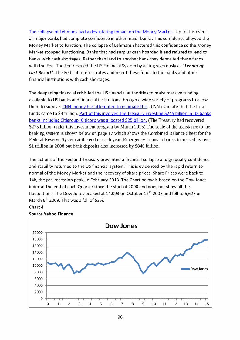
96

The collapse of Lehmans had a devastating impact on the Money Market. Up to this event

all major banks had complete confidence in other major banks. This confidence allowed the

Money Market to function. The collapse of Lehmans shattered this confidence so the Money

Market stopped functioning. Banks that had surplus cash hoarded it and refused to lend to

banks with cash shortages. Rather than lend to another bank they deposited these funds

with the Fed. The Fed rescued the US Financial System by acting vigorously as “Lender of

Last Resort”. The Fed cut interest rates and relent these funds to the banks and other

financial institutions with cash shortages.

The deepening financial crisis led the US financial authorities to make massive funding

available to US banks and financial institutions through a wide variety of programs to allow

them to survive. CNN money has attempted to estimate this . CNN estimate that the total

funds came to $3 trillion. Part of this involved the Treasury investing $245 billion in US banks

banks including Citigroup. Citicorp was allocated $25 billion. (The Treasury had recovered

$275 billion under this investment program by March 2015).The scale of the assistance to the

banking system is shown below on page 17 which shows the Combined Balance Sheet for the

Federal Reserve System at the end of each year. Emergency Loans to banks increased by over

$1 trillion in 2008 but bank deposits also increased by $840 billion.

The actions of the Fed and Treasury prevented a financial collapse and gradually confidence

and stability returned to the US financial system. This is evidenced by the rapid return to

normal of the Money Market and the recovery of share prices. Share Prices were back to

14k, the pre-recession peak, in February 2013. The Chart below is based on the Dow Jones

index at the end of each Quarter since the start of 2000 and does not show all the

fluctuations. The Dow Jones peaked at 14,093 on October 12th 2007 and fell to 6,627 on

March 6th 2009. This was a fall of 53%.

Chart 4

Source Yahoo Finance

0

2000

4000

6000

8000

10000

12000

14000

16000

18000

20000

0 1 2 3 4 5 6 7 8 9 10 11 12 13 14 15

Dow Jones

Dow Jones

97

During the Financial Crisis it became obvious that the repeal of the 1933 Glass-Steagal Act

by the GLBA Act of 1999, which allowed banks to get involved in a variety of high risk areas

including proprietary trading in complex derivatives, had contributed to the financial

instability .The Dodd-Frank’s Act of 2010 introduced restrictions on the activities of US

banks to prevent them from engaging in such high risk activities. One section of the Dodd-

Franks Act, known as the Volker Rule, restrains banks from short-term proprietary trading of

securities, derivatives, commodity futures and options on these instruments .

Following on from the Financial Crisis the Fed, in line with the development of the Basel 3

Rules and the requirements of the 2010 Dodd-Franks Act, introduced new Capital Ratios and

Liquidity Requirements for US institutions. The Capital Ratio requires banks to have capital

equal to 8% of Risk Weighted Assets. The Liquidity Requirements involve having liquid assets

to cover 30 days potential outflows under stressed conditions

Davis Polk have a tool to calculate the risk weighting of assets of US banks. Some assets,

such as cash and deposits with the central bank, which have no risk, have a 0% weighting

and payments due to the bank which are delayed beyond 46 days have a 1,250% weighting.

This means that two banks with the same amount of assets can end up with significantly

different Risk-Weighted Assets. The table below gives an outline of Risk Weighting for Basel

3 for US banks and is based on the Davis Polk Risk Weighting Tool.

Assets Class US Risk Weighting

Cash and Deposits with the Federal Reserve 0%

Residential Mortgages, 50%

Publically-traded Equities 300%

High risk Equities 600%

Payments due delayed beyond 46 days 1,250%

In early 2015 the Fed carried out special Stress testing of the 6 largest banks in the US.

These banks are JP Morgan Chase, Bank of America, Citigroup, Wells Fargo, Goldman Sachs

and Morgan Stanley. These tests revealed that under severe stress conditions that Goldman

Sachs, JP Morgan and Morgan Stanley would hold inadequate capital. This forced these

three banks to reduces their planned dividend payments or share buybacks

Monetary Policy

The Federal Reserve Website explains that “"monetary policy" refers to the actions

undertaken by a central bank, such as the Federal Reserve, to influence the availability and

cost of money and credit to help promote national economic goals. The Federal Reserve Act

of 1913 gave the Federal Reserve responsibility for setting monetary policy”.

98

The Federal Reserve’s responsibility for managing monetary policy comes from the 1913

Act’s Preamble which directed the Fed "to furnish an elastic currency”.

The Fed’s role in Monetary Policy was clarified by Federal Reserve Act in 1977 which

directed the Fed to "maintain long run growth of monetary and credit aggregates … so as to

promote effectively the goals of maximum employment, stable prices, and moderate long-

term interest rates". This wording, which focused on Monetary and Credit aggregates,

reflected the thinking in the 1970s (Monetarism) which argued that the role of a central

bank was to control the economy and particularly inflation by focusing on “Monetary

Aggregates” such as M1 and Credit Growth.

However all attempts to control the economy through controlling the money supply with

targets for M1 or other definitions of money were not effective as banks innovated and

technology changed. The first ATM was installed by Barclay’s Bank in London in 1967. The

availability of ATMs reduced the need to hold large amounts of cash. More recent examples

of this innovation and technology change include Internet Banking and Bitcoins.

Ben Bernanke explained this in 2006 “Unfortunately, the empirical relationship between

money growth and variables such as inflation and nominal output growth has continued to

be unstable at times”.

This led the Fed to focus on controlling Interest rates as a way of controlling the economy.

This focus on interest rates, now referred to as “Conventional Monetary Policy” lasted from

the 1980s until the 2008 Financial Crisis. After 2008 the Fed also used Quantitative Easing

and Forward Guidance.

“Conventional Monetary Policy” involves the management of a target short-term interest

rate (In US - the Federal Funds Rate and in UK - the Money Market Rate). “Federal Funds” in

the US are excess reserves held by banks with the Fed. Banks which are short of funds

borrow these excess reserves for short periods including one day. The one day rate of

interest on interbank lending plays a key role in setting interest rates on longer term loans.

The Chart below gives the Fed Funds Rate from 1990 to the present. The chart is based on

the Fed Funds rate at the end of each quarter.

99

Chart 5

The New York Fed implements the Fed’s Open Market Operations and this link to the New

York Fed Website gives the daily Fed Funds Rate.

In general longer term interest rates tend to fall when the short-term rate falls and tend to

rise when the short-term rises. Lower long-term interest rates encourage purchases of long-

lasting consumer goods, houses, and capital goods and discourage saving. When the Central

Bank cuts the short-term rate it stimulates the economy. When the Central Bank increases

the short-term rate it slows down the economy.

The Federal Reserve controls four tools of monetary policy. These tools are the Discount

Rate, Reserve Ratio, the Interest Rate on Excess Deposits and Open Market Operations

(OMO).

The Board of Governors of the Federal Reserve System is responsible for the Discount Rate,

Excess Reserves Rate and Reserve Requirements and the Federal Open Market Committee

(FOMC) is responsible for Open Market Operations.

The Discount Rate is the interest rate charged to commercial banks and other depository

institutions on loans they receive from their regional Federal Reserve Bank's lending

facility—called the discount window. All “discount window loans” are fully secured. The

Discount Rate is set above the usual level of short-term market interest rates and was at

0.75% in April 2015.

The second tool is Reserve Requirements. US Banks need to have reserves with the Fed for

two reasons:

0

1

2

3

4

5

6

7

8

9

90 91 92 93 94 95 96 97 98 99 0 1 2 3 4 5 6 7 8 9 10 11 12 13 14 15

Fed Funds Interest Rate, %

Fed Funds

100

1 To allow settlements under the “Fedwire” bank settlement system.

2 To meet the Fed’s Minimum Reserve Requirements.

All 9k banks in the US use the Fedwire “clearinghouse” settlement system which handles 45

million items per day with average value of $1.7k.

The Fed Website explains that “Reserve Requirements are the amount of funds that a

depository institution (Bank) must hold in reserve against specified deposit liabilities. Within

limits specified by law, the Board of Governors has sole authority over changes in reserve

requirements. Depository institutions must hold reserves in the form of vault cash or deposits

with Federal Reserve Banks”.

The Federal Reserve Website explains that “The interest rate paid on excess balances is also

determined by the Board and gives the Federal Reserve an additional tool for the conduct of

monetary policy”. That rate was 0.25% in April 2015 but if in the future the Fed wants to

push up the Federal Funds Rate it can do so by offering an attractive interest rate on Excess

Deposits.

The Fed Website explains that “Open Market Operations (OMOs) --the purchase and sale of

securities in the open market--are a key tool used by the Federal Reserve in the

implementation of monetary policy. The Federal Reserve uses OMOs to adjust the supply of

reserve balances so as to keep the Federal Funds Rate--the interest rate at which depository

institutions lend reserve balances to other depository institutions overnight--around the

target established by the FOMC”.

The Federal Reserve Act of 1913 was designed “to provide the nation with a safer, more

flexible, and more stable monetary and financial system”. Traditionally the US Federal

Reserve Bank has attempted to control the Business Cycle in the US Economy using the rate

of interest. The “Fed” attempts to balance the economy to achieve “its long-run goals of

price stability and sustainable economic growth”.

The choices open to the Fed are illustrated by the Table below which illustrates the link

between the Business Cycle, the level of Overall Demand, the level of GNP Growth, the level

of Inflation and the Employment situation. The three examples represent Recession,

Balance and Boom.

Business Cycle Demand Level GNP Growth Inflation Unemployment

Recession Too Low Below 4% Below 2% Rising

Balance Correct Level 4% 2% Full Employment

Boom Excessive Above 4% Above 2% Labor Shortage

101

The Fed normally tries to control the economy through controlling the Federal Funds Rate

or Fed Rate. Commercial banks borrow and lend Excess Reserves at the Fed between each

other without security and the rate at which this money is traded is the “Fed Rate”.

The Federal Open Market Committee (FOMC) sets a target for the “Fed Rate” and tries to

achieve this target by Open Market Operations. Open Market Operations involve the Fed

buying and selling US Government Securities. Open Market Operations change the amount

of “Liquidity” held by the commercial banks. When, for example, the Fed sells a Government

Security the buyer will normally use a bank deposit to pay for the security. The payment will

involve the purchaser’s bank making a liquidity transfer (cash or deposits with Fed) to the

Fed. This reduces the amount of liquidity within the banking system and is likely to lead to a

rise in the Fed Funds Rate.

The Discount Rate is the rate at which the Federal Reserve lends to commercial banks. The

Fed always keeps the Discount rate just above the Fed Funds Target Rate.

The Fed Discount Rate and Fed Funds Rate from 2003 to 2015

Chart 5

The chart above is based on the Discount Rate and the Fed Funds Rate at the end of each

Quarter.

If the economy is in balance the Fed will pursue what is called a neutral interest rate policy.

A 4% Fed Rate is normally regarded as neutral. A rate below 4% is often described as

“expansionary” or “accommodative” and a rate above 4% is described as “restrictive”.

Before the 2007 Financial Crisis the Fed Rate was 5.25%. The Fed cut the Fed Rate rapidly to

a range from 0.0% to 0.25% in December 2008. This is the lowest rate ever in the history of

the Fed and indicates a severe recession with inadequate Demand and with the danger of

0

1

2

3

4

5

6

7

3 4 5 6 7 8 9 10 11 12 13 14 15

Fed Discount Rate

Fed Funds Rate

102

inflation being replaced by a danger of deflation. The Fed has continued with the 0.25 Fed

Funds rate until May 2015.

US Fed Funds Rate Cycle

1990 1993 2000 2003 2007 2008 2015

High Rate 8.0% 6.5% 5.25%

Low Rate 3.0% 1.0% <0.25%

Taylor Rule

Up until 2009 the Fed did not state its Target GDP Growth Rate or Target Inflation Rate.

The thinking in the Fed appeared to be in lines with the Taylor Rule which was devised by

John Taylor of Princeton University.

The Taylor Rule is:

Fed Rate = 4% + 1.5 (Actual GDP Growth - Target GDP Growth + Actual Inflation - Target

Inflation)

The Target GDP Growth was the Long-term Sustainable Growth Rate of 4% and the Target

Inflation Rate was 2%. Using these targets gives us the Fed Rate as follows

Fed Rate = 4% + 1.5 (Actual GDP Growth - 4 + Actual Inflation - 2)

The Taylor Rule gives a Fed Rate of 4% (seen as a neutral rate) if the GDP Growth Rate is 4%

and the Inflation Rate is 2% but if the overall level of demand is too high, resulting in a GDP

growth rate higher than 4% and inflation above 2%, then the Fed Rate must rise, eg if GDP

growth is 5% and inflation is 3% then the Fed Rate should rise to 7%.

The Taylor Rule shows how interest rate should move in a normal business cycle however

the crisis in finance and the scale of the recession in 2008/09 was outside this normal cycle.

GDP fell by 2.8% and prices fell by 0.3% in 2009. Applying the Taylor Rule to this situation

would have given a 2009 Fed Rate = 4 + 1.5(-2.8 -4 -0.3 – 2) = 4 + 1.5(-9.1) = -10

This means that the Taylor Rule applied in 2009 would have given a Fed Funds rate of -10%.

This would mean that a bank would have to pay another bank 10% pa to hold its money for

it and this is not realistic as it is impossible to drive down interbank rates or the Fed Funds

rate much below 0%.

The scale of the Financial Crisis was so great that the US economy contracted rapidly at the

end of 2008. The impact of this on employment is shown in Chart 6 which is based on US

Unemployment at the end of each quarter. US Unemployment rose from 4.4% in early 2007

to 10.0% in October 2010.

103

Chart 6

A cut in the Fed Funds Rate to near zero was insufficient to stimulate consumer and

investment spending. The low level of demand was leading to a build-up of stocks

(inventory), cash flow problems for business and a rapid rise in unemployment. The low

level of demand was also creating a risk of long-term deflation. This led to the Fed to adopt

“Unconventional Monetary Policy” tools. These were Quantitative Easing and Forward

Guidance.

Quantitative Easing

“Quantitative Easing” (QE) is an “Unconventional Monetary Policy” used by central banks to

stimulate the economy when standard monetary policy has become ineffective. A central

bank implements quantitative easing by increasing the money supply. It does this by

buying financial assets from commercial banks and other private institutions. By buying

these assets and bidding up their price the central bank also lowers the yield on these

assets.

US Quarterly %∆ in GDP and Inflation from 2008 to 2014

Chart 7

0

2

4

6

8

10

12

4, Q1 5, Q1 6, Q1 7, Q1 8. Q1 9, Q1 10, Q1 11, Q1 12, Q1 13, Q1 14,Q1 15, Q1

US Unemployment Rate %

US Unemp

-10

-8

-6

-4

-2

0

2

4

6

8 9 10 11 12 13 14 15

%∆ in GDP

Inflation

104

The Chart above with GDP figures from the Bureau of Economic Analysis and prices (CPI

Unadjusted) from the Bureaux of Labor Statistics shows that the US economy contracted by

8.3% in the last quarter of 2008. This rapid contraction led the Fed to start buying bonds

and other securities in November 2008. This is now referred to as QE1. The Fed started QE 2

in November 2010 because the economy was not recovering as expected. The Fed started

QE 3 in September 2012 as the economy was still not recovering. QE 3 involved asset

purchases of $85 billion per month. The Fed ended its QE 3 program of asset purchases in

October 2014.

Under the QE programs the Fed purchased Treasury Bonds (US Government) and

government-sponsored enterprise (GSEs) Mortgage Backed Securities to push down long

term interest rates. These actions also massively increased the Fed’s Balance Sheet as

shown below in a summary extracted for the Annual Combined Accounts. The Emergency

lending to the banks in 2008 was phased out and replaced by increased purchasing of

Treasuries and Mortgage Backed Securities issued by Government Sponsored Enterprises

such as Fannie Mae and Freddie Mac.

Federal Reserve System Combined Balance Sheet in $ billions

Assets 2007 2008 2009 2010 2011 2012 2013 2014

Treasuries 47 80 805 1066 1750 1809 2356 2416

MBS 745 502 919 1004 848 950 1533 1734

Emergency Loans 73 1098 96 0 0 0 0 0

Other 50 566 415 357 320 158 135 297

Total 915 2246 2235 2427 2918 2917 4024 4492

Liabilities

Notes 792 853 888 942 1034 1126 1197 1267

Bank Deposits 21 860 977 968 1562 1491 2249 2796

Other 102 533 370 517 322 300 578 429

Total 915 2246 2235 2427 2918 2917 4024 4492

The growth in the Fed’s Assets is shown in this Graph from the Wall Street Journal below.

105

Ben Bernanke explained the impact of QE on interest rates in the following words “With the

available supply of Treasury and GSE securities reduced by Fed purchases, investors were

willing (forced) to accept lower yields. Lower longer-term rates helped stimulate the

economy, just as they do under conventional policies. Reduced availability of Treasury and

GSE securities led investors to purchase other assets, such as corporate bonds, lowering the

yields on those assets as well”.

The impact of QE on long term interest rates can be seen by looking at 10 and 30 year bond

yields. The Yield on 10 Year US Treasury Bonds fell to 2% and the Yield on 30 Year US

Treasury Bonds fell to below 3%.

Chart 8

US Treasury 10 year Bond Yields

Source Yahoo Finance

106

Chart 9

US 30 year Bond Rates

The 30 year bond yield graph, however, shows that even with this massive program of Asset

Purchase it was not possible for the Fed to keep Long Term Bond Yields much below 3%.

Forward Guidance

The Fed has been using Forward Guidance since 2011 as a tool of monetary policy. Forward

Guidance involves the Fed, or any central bank, giving a clear and transparent assessment of

its judgment on the direction of interest rates movement into the future.

The Fed has used Forward Guidance to drive down medium-term interest rates by signaling

that they planned to keep short-term interest rates at a low level for an extended period.

When the Fed indicated that they were committed to keeping short-term interest rates low

for a considerable period it signaled to the market that there was a much reduced risk to

lenders for the medium term that they would be caught by a rise in short-term rates. This

helped to reduce medium term interest rates.

John Williams, President of the San Francisco Fed explained the impact of Forward guidance

as follows in a speech he delivered in November 2012 “The introduction of forward guidance

in the August 2011 FOMC statement succeeded in shifting market expectations regarding

the future path of the federal funds rate. Specifically, the FOMC stated that it “anticipates

that economic conditions…are likely to warrant exceptionally low levels for the federal funds

107

rate at least through mid-2013.” That statement communicated that the FOMC would

probably keep the fed funds rate near zero for at least two more years, longer than many

private-sector economists had been thinking. As a result of this shift in expectations, yields

on Treasury securities fell by between one- and two-tenths of a percentage point”.

The Bank of England and the ECB both followed the lead of the Fed in adopting Forward

Guidance as a Monetary Policy Tool.

Inflation Target

As a step towards greater transparency the Fed Chairman Ben Bernanke announced in

February 2009, in the context of severe deflationary pressures in the US economy, that the

Fed would set a target inflation rate of 2%. This was the rate which was always assumed to

be the Fed’s Target Inflation Rate.

There was a fear that the increase in the Money Supply caused by Quantitative Easing would

cause inflation as per Fishers Equation, MV = PT but this has not happened. Chart 7 above

shows that the inflation rate for 2013 and 2014 was below 2%. Even the German

Bundesbank which was afraid that similar Quantitative Easing by the ECB would generate

inflation is now will to accept Quantitative Easing.

However the increase in the Money Supply has increased Asset Prices by bringing down

interest rates. This has benefitted the owners of assets, such as shares (chart below) and

property, and therefore has shifted wealth in favor of those who were already wealthy.

Economic Recovery

The Dow Jones Index which reached a peak at almost 14k in October 2007 fell by over 50%

to below 7k in March 2009 but reached 14k again in March 2013

Chart 10

6,627 in March 2009

14,093 in October 2007

108

The recovery in share prices in 4 years contrasts with the recovery after the Great

Depression which took 30 years - until 1959. The table below contrasts the Great Recession

with the Great Depression.

Factor Great Depression Great Recession

Fall in Dow from Maximum to Minimum 85% 53%

Length of time until full recovery in Dow 30 Years 4 Years

Length of Recession 4 Years 1 Year

Bank Deposits lost Deposits in 10k Banks None

Decline in GDP 33% 4%

The US economy has been recovering with a GDP Growth of 2.6% in 2013 and good growth

in early 2014. This happened with Inflation still below the Fed Target. The Fed decided in

December 2013 to run down its Asset Purchase Program during 2014 ending in October

2014.

Over the next two years the Fed is likely to reverse QE by large scale selling of its Assets. It

will also increase the Federal Funds Rate broadly in line with the Taylor Rule although how

to apply the Taylor Rule as the economy comes out of this dramatic recession may be

complex. There are also indications that the Fed is now focusing more on the

unemployment rate than on the growth rate. The Fed Game below has replaced the GDP

Growth Target of 4% by a 5% Unemployment Target.

But whatever targets the Fed sets it is likely that the Fed Funds Rate will increase

significantly during 2015.

The Fed has a simple game for students showing how Monetary Policy Works . This site is

worth visiting.

109

The European Union and its currency

Introduction

This note covers the History of the European Union, EU Institutions, Introduction of the

Euro, History of the Eurozone, the ECB, Financial Stability in the Eurozone, ECB Monetary

Policy, Forward Guidance, Quantitative Easing, Shared Approach to Bank Resolution, Euro

Exchange Rate and the Impact of the Recession on the operation of the Eurozone and ECB.

History of the European Union

The foundations for the EU were laid in the years after the ending of Second World War.

This war which involved Germany, Japan and Italy on one side and the US, UK and the Soviet

Union on the other side, lasted from 1939 to 1945 and killed tens of millions worldwide and

devastated Europe, China and Japan.

In the immediate aftermath of the war Western European political leaders sought to

develop a European Economic Community (EEC) which would contribute to the economic

recovery of Western Europe, prevent another war between France and Germany and

prevent the takeover of the free democratic countries of Western Europe by the Soviet

Union and its communist allies.

France and Germany had fought three wars in 1870-71 (Franco- Prussian), 1914-18 (WW1)

and 1940-45 (WW2). After the end of World War 2 the Soviet Union and the West (Western

Europe and the US) fought a “Cold War” and the threat of Communist expansion

encouraged France and Germany to end their historic rivalry. Europe was divided by what

was called the “Iron Curtain” separating the “Free Countries” of Western Europe and the

Soviet Union dominated Communist Bloc. The formation of the EEC was strongly supported

by the US. The US considered that a strong European Partner was vital to US attempts to

curb communist expansion.

The six founding members of the EEC were France, Germany, Italy, Belgium, Holland and

Luxembourg. These six countries formed the European Coal and Steel Community (ECSC) in

1951 and then proceeded to set up European Economic Community (EEC) in 1958. Since the

1950s the community, now referred to as the European Union (EU), has grown by adding

new member countries and new powers. There are now 28 member countries including all

the countries of Western Europe, apart from Switzerland, Iceland and Norway, and many

Eastern European countries including 10 countries that were formerly part of the

Communist Bloc.

The EU, in 2014, has a combined population of over 500 million and generates about 20% of

global GDP.

110

The EU has also grown in power by agreeing new treaties giving new additional roles to the

community. The EU developed a single market through a standardized system of laws that

apply in all member states and the elimination of trade restrictions. EU policies aim to

ensure the free movement of people, goods, services, and capital and maintain common

policies on trade including agriculture.

The EU has developed a limited role in external relations and defense through a Common

Foreign and Security Policy.

The EU has also developed a monetary union, known as the Eurozone. The Eurozone was

established in 1999 and came into full force in 2002 with the introduction of the Euro as the

currency of 11 countries. The Eurozone is currently composed of 18 member states that use

the Euro as their legal tender. The European Central Bank is the Central Bank of the

Eurozone.

EU Institutions

The European Union (EU) is an economic and political union of 28 European countries. The

EU operates through a system of independent supranational institutions. These institutions

are the European Commission, the Council of the European Union, the Court of Justice of

the European Union, the European Central Bank, the Court of Auditors and the European

Parliament. The European Parliament is elected every five years by EU citizens.

All major decisions within the EU require unanimous agreement of all 28 member countries.

Member countries differ in level of commitment to the community, legal frameworks,

culture and level of economic development.

The UK, for example, has always been a reluctant member of the EU, remains outside the

Eurozone and is even planning a Referendum on continuing its membership. Ireland has a

constitution that requires that all international agreements that impact on the constitution

have to be put to a popular referendum. Germany has a powerful Constitutional Court and

all agreements by the EU and all major decisions by EU institutions have to be consistent

with the Constitutional Court’s interpretation of the German Constitution. There are

significant cultural differences between Northern and Southern Europe. This is particularly

true in terms of attitude to inflation with most Northern European Countries strongly

opposed to inflation. Northern Europe has a much more developed economic system

compared to Southern and Eastern Europe.

These differences between EU member countries mean that decision-making within the EU

is slow and complex and requires a long process of consensus building. This was shown by

the EU response to the Financial Crisis. The ECB has a timeline of this response which shows

the slowness and complexity of this response.

111

The EU response to the Financial Crisis in 2007/08 was much slower and less decisive than

that of the US, Japan and China. When the banking systems in Ireland, which is within the

Eurozone, and the UK, which is outside the Eurozone, were threatened by financial panic

both governments intervened to protect their banking systems without consulting the

European Central Bank (ECB). The ECB even increased interest rates during 2008 while the

crisis was developing. The US, UK and Japan introduced Quantitative Easing (QE) in 2008 -

2009. Germany and some other North European countries opposed the ECB doing QE on the

basis that it would cause inflation. This delayed Eurozone QE until the start of 2015 when it

was clear that QE did not cause immediate inflation in either the US, Japan or Britain.

The inadequate EU response to the financial crisis, particularly when it almost bankrupted

some Eurozone countries, even threatened the survival of the Euro and the Eurozone. The

ECB however has moved slowly forward in addressing the financial crisis in the Eurozone

and the survival of the Eurozone is no longer threatened.

Introduction of the Euro

In the early years of the EEC all the major member states had their own currencies. The

value of these currencies could change on the Foreign Exchange. The EEC therefore used the

$US to keep accounts and measure financial transactions. In 1971, US President Richard

Nixon removed the gold backing from the $, causing a collapse in the Bretton Woods

System that had provided international financial stability since 1945. The Nixon decision led

to a fluctuations in exchange rates and a fall in the value of the $. The EEC started to use a

European Unit of Account (EUA), based on the pre-devaluation $, for accounting purposes.

In 1978 the EEC decided to set up the European Monetary System (EMS). This involved a

New Currency Unit called the European Currency Unit (ECU) but based on the EUA or pre

1971 $, fixed Exchange Rates for EMS currencies based on the ECU and a new organization

called the European Monetary Cooperation Fund (EMCF).

Ireland agreed a value for the Irish Pound of IR£0.66 = ECU with Germany agreeing a

DM2.51 = ECU. This gave a value for the IR£ = DM3.80. Britain stayed out of the EMS until

October 1990 and then joined with £Stg0.70 = ECU. In September 1992 (Wednesday

16/9/1992, “Black Wednesday”) Britain was forced to leave the EMS by Foreign Exchange

speculation, including major activity by George Soros. Britain allowed its currency to float

down against EMS Currencies. Britain’s withdrawal from the EMS was a major setback and

showed the problems associated with partial monetary union.

Germany had been divided between East Germany, part of the Communist Bloc, and West

Germany, part of Western Europe, since the end of World War 2. The fall of Communism in

1989/90 led to the collapse of the communist regime in East Germany and a desire among

almost all Germans for re-unification of Germany. There was significant international

opposition, particularly in France and Britain to the re-unification of Germany. This

112

opposition was based on the fear that a re-unified Germany would come to dominate

Europe. There was also opposition in Germany to the creation of a single European currency

to replace, in Germany, the Deutschmark. A political deal was negotiated, at a summit

meeting in Dublin, in 1990 that involved Germany agreeing to the setting up of a single

European currency in exchange for European Union (EU) support for German re-unification.

The decision by the German Government to replace the Deutschmark with the Euro was not

supported by a majority of Germans. Germans were very proud of the Deutschmark. The

Deutschmark had been one of the strongest currencies in the world over the period 1960 to

1990 and had helped to establish financial stability in Germany. The German government

agreed to replace the Deutschmark by the Euro but would not agree to the undermining of

the Bundesbank’s (German Central Bank) role in supervising and controlling the German

banking system. This led to a situation where the ECB was in charge of Monetary Policy but

the national central banks were in charge of Financial Stability Policy (controlling the

financial system).

The goal of achieving Economic and Monetary Union (EMU) in Europe including a single

currency was enshrined in the 1992 Maastricht Treaty (Treaty on European Union), which

set out the ground rules for its introduction. These stated the objectives of EMU, allocated

responsibly for setting up the Euro and specified the conditions Member States must have

met in order to adopt the Euro. These conditions were known as the 'convergence criteria'

(or 'Maastricht criteria') and included low and stable inflation, exchange rate stability and

sound public finances. The European Monetary Institute (EMI) was set up in 1995 under the

Masastricht Treaty to prepare for full monetary union.

In 1997 the EU agreed a Stability and Growth Pact, designed to ensure budgetary discipline

after creation of the euro. To participate in the new currency, member states had to

meet strict criteria such as a budget deficit of less than 3% of their GDP, a debt ratio of less

than 60% of GDP, low inflation and interest rates close to the EU average. In 1998 the EU

agreed the 11 countries that were to take part in the launch of the Euro. Greece applied to

join the Euro but failed to meet the criteria and was excluded from the Eurozone. There was

a penalty clause in the Stability and Growth Pact but this was not enforced by the EU against

France and Germany who both had budget deficits in excess of 3% in 2003 and 2004.

The EMI chose the name Euro for the new currency and agreed to launch the new currency

on January 1st 1999. The value of the Euro was based on the ECU. The European Central

Bank was set up to control the new currency and take over from the European Monetary

Institute.

113

The conversion rates between the original 11 participating national currencies and the Euro

were established in 1998. On 1 January 1999 the national currencies of the 11 participating

countries (the Eurozone) were locked at fixed rates against each other. The notes and coins

for the old currencies, however, continued to be used as legal tender until Euro Notes were

introduced on 1 January 2002. All other money forms including bank deposits, loans and

government bonds were converted into the Euro on January 1st 2002. The transition went

smoothly and within two weeks the Euro was the accepted currency in all Eurozone

countries.

The original 11 countries that set up the Euro were Belgium, Germany, Ireland, Spain,

France, Italy, Luxembourg, the Netherlands, Austria, Portugal and Finland. Since then 7

other countries have joined. These 7 are Greece (which joined in 2002), Slovenia, Cyprus,

Malta, Slovakia, Estonia, Latvia and Lithuania. Lithuania only joined on 1st January 2015.This

means that the euro is the currency of 19 countries and is used by 330 million people as

their currency.

Denmark has locked its currency, the Krone (DKK), against the € but has continued to use its

own currency. Two non EU countries, Montenegro and Kosovo have adopted the € without

membership of the EU or the Eurozone.

The UK, Sweden, Poland, the Czech Republic, Slovenia, Bulgaria and Romania are members

of the EU but have not adopted the €.

In the countries using the € the traditional role of a central bank was divided between the

European Central Bank (ECB) and the central bank of each country. In Ireland, for example,

this meant that the Currency Role and Monetary Policy were controlled by the ECB and the

EU states using the euro (Eurozone) Euro linked currency Other EU states Non EU States using the euro This map is slightly out of date as Lithuania joined the Euro on 1/1/2015

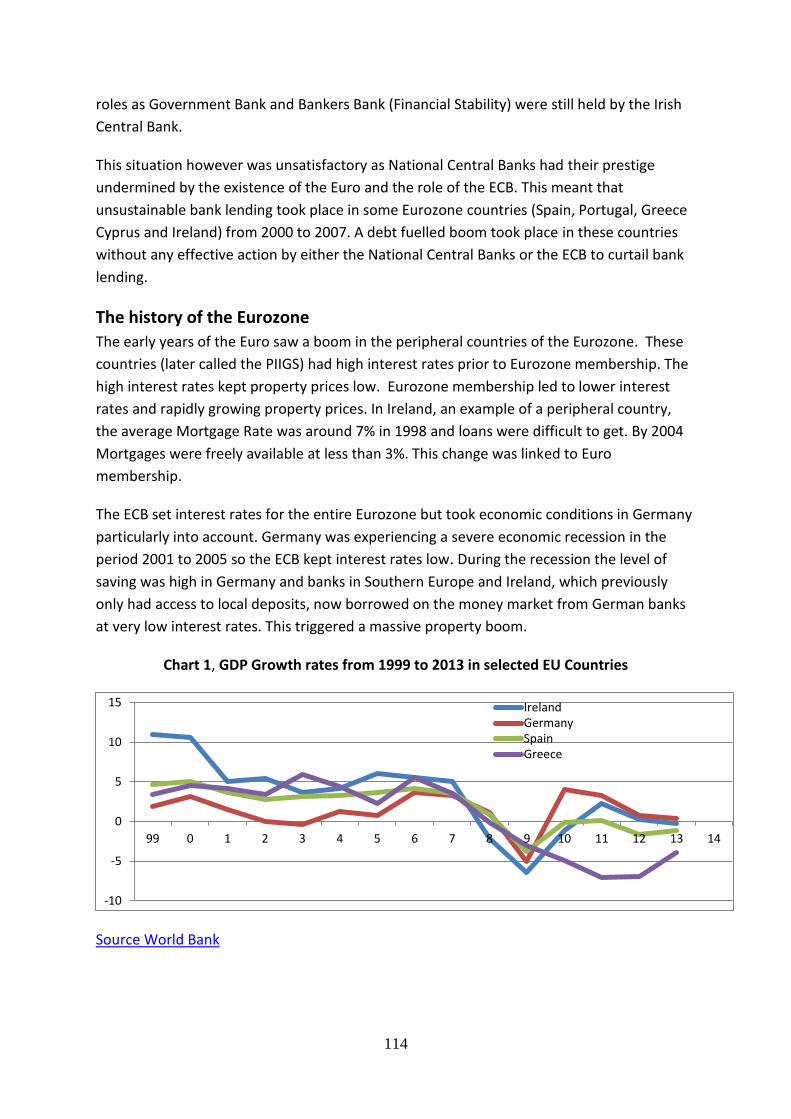
114

roles as Government Bank and Bankers Bank (Financial Stability) were still held by the Irish

Central Bank.

This situation however was unsatisfactory as National Central Banks had their prestige

undermined by the existence of the Euro and the role of the ECB. This meant that

unsustainable bank lending took place in some Eurozone countries (Spain, Portugal, Greece

Cyprus and Ireland) from 2000 to 2007. A debt fuelled boom took place in these countries

without any effective action by either the National Central Banks or the ECB to curtail bank

lending.

The history of the Eurozone

The early years of the Euro saw a boom in the peripheral countries of the Eurozone. These

countries (later called the PIIGS) had high interest rates prior to Eurozone membership. The

high interest rates kept property prices low. Eurozone membership led to lower interest

rates and rapidly growing property prices. In Ireland, an example of a peripheral country,

the average Mortgage Rate was around 7% in 1998 and loans were difficult to get. By 2004

Mortgages were freely available at less than 3%. This change was linked to Euro

membership.

The ECB set interest rates for the entire Eurozone but took economic conditions in Germany

particularly into account. Germany was experiencing a severe economic recession in the

period 2001 to 2005 so the ECB kept interest rates low. During the recession the level of

saving was high in Germany and banks in Southern Europe and Ireland, which previously

only had access to local deposits, now borrowed on the money market from German banks

at very low interest rates. This triggered a massive property boom.

Chart 1, GDP Growth rates from 1999 to 2013 in selected EU Countries

Source World Bank

-10

-5

0

5

10

15

99 0 1 2 3 4 5 6 7 8 9 10 11 12 13 14

IrelandGermanySpainGreece

115

In 2006, for example, the ECB Rate was 2% while Irish GDP Growth was 5.5% and Spanish

growth was 4.1%. An independent central bank in Ireland or Spain at that time would have

pushed up interest rates to control the excessive demand.

In Ireland in 2006 the Irish GDP Growth of 5.5% was combined with a 2.5% inflation rate.

The Taylor Rule [Fed Rate = 4% + 1.5 (Actual GDP Growth - Target GDP Growth + Actual

Inflation - Target Inflation )]would have suggested a Central Bank Rate of 7.0% as

appropriate for Ireland but the ECB Rate was only 2%.

Chart 2, Irish GDP Growth, Inflation and ECB Refi Rate from 1999 to 2014

The imbalance between the actual interest rates and the interest rate appropriate to the

needs of their economies led to a property boom in Southern Europe and Ireland. Irish

banks could borrow Euros easily at the ECB Refi Rate and were willing to lend at ECB Refi

Rate + 1%. This gave an Irish Mortgage Rate of 3% while house prices were rising at 20% per

annum. The property boom led to an increase in average house prices from €78k in 1995 to

€306k in 2006. House and apartment building boomed and reached 90k in 2006 while the

birth rate was only 65k.

The Irish Central Bank and the ECB did nothing to try and prevent this excessive boom. This

failure by the ECB and Irish Central Bank eventually led to greatest economic and financial

crisis in the history of the state. The crisis came to a head on September 29th 2008. That

morning the Chairman of Ireland’s third largest bank, Anglo Irish Bank, contacted the

Chairmen of the two largest banks, Bank of Ireland and AIB, asking for an emergency short-

term loan as Anglo Irish had to repay over €1 billion the following morning and did not have

the funds and could not borrow on the money market and could not get funds from the Irish

Central Bank. (Anglo-Irish was also suffering a run on its deposits and lost €1.8 billion of

deposits on that day alone). This would mean that the third largest bank in Ireland could

-10

-5

0

5

10

15

99 2000 1 2 3 4 5 6 7 8 9 2010 11 12 13 14

ECB Refi Rate

Irish Inflation

Irish GDP Growth

116

not open in the morning. The Chairmen and Chief Executives of Ireland’s two largest banks

then sought an emergency meeting with the Government. That meeting lasted most of the

night.

During that meeting the Irish Government decided to issue a “blanket guarantee” covering

all the liabilities of the Irish banks (€450 billion) based on the belief that the banks were

suffering a liquidity problem. It turned out that the Irish banks were insolvent and that

decision has cost the Irish state €64 billion.

The two leading banks in Ireland, AIB and Bank of Ireland had to be rescued by the State and

their shareholders lost 99% of their investment. The third and sixth largest banks in Ireland,

Anglo-Irish and Irish Nationwide, went bankrupt completely wiping out shareholders. The

fourth and fifth largest banks, Ulster and National Irish, which were subsidiaries of foreign

banks, had to be rescued by their parent banks. In the case of Ulster Bank its parent bank,

the RBS which saved Ulster by an injection of £16 billion, had itself to be rescued by a £46

billion injection from the British Treasury. National Irish, a subsidiary of the Danish bank,

Danske, also required significant funding from its parent to survive.

The Irish economy went into a massive recession at the end of 2008. GDP at Market Prices

fell by 14% in 1989 alone. Building activity fell by 90%. House prices fell by 60%. Consumer

spending fell massively. Government tax revenue fell by 30%. The Government cut public

sector wages and welfare benefits. Businesses collapsed. Unemployment rose sharply. The

rate of interest on Irish 10 year government bonds rose to 15%. Irish share prices fell by 85%

but bank shares fell by 99%. Ireland applied to EU and IMF for a bailout in November 2010.

During 2010 the EU realized that some EU governments would not be able to sell bonds on

the open market and agreed to set up a fund called the European Fiscal Stability Facility

(EFSF). The role of this fund was to provide funding for governments that were unable to

borrow on the open market. The EFSF was agreed in May 2010. The EFSF was allowed to

borrow up to €400 billion and this borrowing was guaranteed by the EU. The EFSF was used

to part fund (with the IMF) the rescue of Greece in May 2010, Ireland in November 2010

and Portugal in May 2011.

The loss of confidence in the Euro during 2011 led to a massive movement into the Swiss

Franc (CHF). This led to an increase in the value of the CHF from €0,62in 2008 to €0.96 in

2011. The 50% increase in the value of the CHF massively damaged the competitiveness of

the Swiss Economy and forced the Swiss National Bank (Central Bank) to intervene to put an

upward cap on the value of the currency at CHF1.2 = €1 or CHF1 = €0.83. The Swiss National

Bank maintained this cap on the value of the CHF until January 2015 when the weakness of

the €, linked to Eurozone Quantitative Easing, forced the Swiss to end the cap. The

immediate reaction was a rise in the value of the CHF from €0.83 to €0.96. This led to an

immediate fall of 10% in share prices on the Zurich Stock Market.

117

During 2012 the financial crisis continued in Greece, which required a second Bailout in

early 2013, and threatened to spread to Spain and Italy. There appeared to be a strong

possibility that Greece would leave the Euro and a financial crisis in Italy might require more

funds that those available under the EFSF. In 2012 the EU agreed a Fiscal Compact, which is

effectively a tightening up of the Stability and Growth Pact. Under the Fiscal Compact all

Eurozone countries agreed to:

- achieve Balanced Budgets (this actually involves a budget deficit of less than 3% of

GDP,

- Keep National Debt below 60% of GDP and if above this reducing the excess by 5%

pa,

- Agree a Medium Term Objective with EU Commission and keep its budget in line

with the Medium Term Objective,

- Make the Fiscal Compact part of National Law.

The Fiscal Compact came into force on January 1 2013. All Eurozone countries, and some

other EU member countries, signed the Fiscal Compact. Some EU countries including the UK

did not sign the treaty.

The Fiscal Compact set up a permanent fund called the European Stability Mechanism to

provide funding for emergency loans to governments.

The Cyprus Banking System collapsed in March 2013 as Greece needed a second bailout. As

part of the second Greek bailout (€130bn in addition to the €110bn of the first bailout) the

IMF and EU imposed a write off of 50% on Greek bonds. Cyprus had developed a large off-

shore banking industry largely based on Russian Investors. The Cypriot banks had used these

deposits to fund massive lending to property investors and also invested heavily in Greek

government bonds. The collapse in property prices in Cyprus put these banks under

pressure. The write-off on Greek bonds bankrupted the banks in Cyprus forcing them to

close for two weeks (including ATMs) and forced Cyprus to seek a bailout. As part of that

bailout, Lariki, the second largest bank in Cyprus was closed down and uninsured deposits

suffered significant losses. Deposits up to €100k were protected but 37% of all deposits

above €100 were transformed into shareholding in the banks and these are largely

worthless.

Ireland emerged from the EU/IMF bailout in December 2013 and started to raise funds in

early 2014 on the open market. The rate of interest on these 10 year Irish Government

bonds is 1.5% as November 2014. (The discussion of Ireland is used to illustrate the position

of all the PIIGS)

The ECB

The European Central Bank (ECB) is the Central Bank for the Euro and controls the monetary

policy of the Eurozone. The ECB is one of the world's most important Central Banks and is

118

one of the 7 legal institutions of the European Union (EU). The ECB was established by the

Treaty of Amsterdam in 1998, and is headquartered in Frankfurt, Germany. The ECB was

given complete autonomy in the operation of monetary policy in the Eurozone by the

Amsterdam Treaty.

The President of the ECB is Mario Draghi, former Governor of the Bank of Italy. The owners

and shareholders of the European Central Bank are the central banks of the 28 member

states of the EU. The Directors of the ECB are the Governors of the National Central Banks of

the 18 Eurozone countries.

The primary objective of the European Central Bank, as mandated in Article 2 of the Statute

of the ECB, is to maintain price stability within the Eurozone. The basic tasks, as defined in

Article 3 of the Statute are to define and implement the monetary policy for the Eurozone,

to conduct foreign exchange operations, to manage the foreign reserves of the European

System of Central Banks and manage the financial market infrastructure of the Eurozone.

The ECB’s capital is five billion euro held by the national central banks of the member states

as shareholders. The initial capital allocation was determined in 1998 on the basis of the

each state's population and GDP. Shares in the ECB are not transferable and cannot be used

as collateral.

Financial Stability in the Eurozone

Financial Stability is very difficult to define. The ECB defined financial stability “as a

condition in which the financial system – intermediaries, markets and market infrastructures

– can withstand shocks without major disruption in financial intermediation and in the

effective allocation of savings to productive investment” in its 2014 Financial Stability

Report. The Eurozone has had to face significant financial instability over the period 2008 to

2014 partly due to the weaknesses in the original Eurozone structure.

One of the key weaknesses within the Eurozone, as it was set up in 1999, in addition to

setting interest rates to primarily suit the German economy, was that each member country,

through its own central bank, regulated its banks according to its own laws and banking

rules. This weakness made it very difficult for the Eurozone to deal with the Financial Crisis

in 2007/08. National central banks provided liquidity to their own banks and operated their

own Bank Resolution procedures.

Each national central bank provided liquidity to their commercial banks. This was not a

problem between 1999 and 2007. The problems in Ireland and Southern Europe in 2007

however were such that these countries’ central banks could not provide sufficient funding

for their banks and each central bank, in turn, had to call the ECB for help.

The financial crisis in the US in August/September 2007 created a situation where the

Eurozone money market stopped working. This meant that banks from all over the Eurozone

119

had to borrow from the ECB as Lender of Last Resort). On one day, August 9th 2007, the ECB

lent €97 billion to banks. Because the bank funding crisis was so severe the ECB started to

lend for 3 to 6 months to the banks. It committed itself to provide unlimited funding against

collateral, increased the range of assets it accepted as collateral and started to lend to over

800 banks compared with the 360 that they had lent to before the crisis. This lending was

against bonds with a minimum Credit Rating. However the ECB has used a “waiver” policy

and given loans against securities without this minimum credit rating for countries

participating in a financial adjustment program agreed with the European Commission such

as Ireland, Portugal and Greece. For example in 2012 the ECB agreed to lend against Greek

Bonds which had a junk bond rating by S&P. However the ECB suspended the waiver for

Greek Bonds in February 2015 when the new Greek Government rejected the agreement

which a previous government had entered into with the European Commission. This has

forced Greek banks to rely on what is called Emergency Liquidity Assistance.

The ECB has a program of Emergency Liquidity Assistance for banks which are not able to

provide acceptable collateral. This lending is by the national central bank of the country and

the national central bank accepts the risk of default. Almost inevitably the banking system in

a Eurozone country, where the country is in financial trouble, will depend on ELA. When a

country gets into financial trouble its government bonds will be downgraded and become

ineligible as collateral for normal ECB loans. Banks, who normally hold significant amounts

of government bonds, cannot use their own government bonds to get ECB funding and will

be forced to borrow through the ELA program. This means that the ECB can put pressure on

governments through control of ELA. In 2010 the Irish banking system was highly dependent

on ELA. A letter from JC Trichet, then President of the ECB, to the Irish Minister for Finance,

which hints at the possible withdrawal of ELA, is widely regarded as the trigger which forced

the Irish Government to apply to the IMF for a bailout in November 2010.

The political, economic and financial crisis in Greece that arose after the election of a radical

left-wing government in January 2015 led to a massive outflow of deposits from Greek

banks and by May 2015 the Greek banks were borrowing over €75 billion under ELA. If the

ECB were to withdraw this ELA support from the Greek banks they would inevitably have to

close. This means that the ECB has considerable negotiating power relative to the Greek

Government just as he had with Ireland in 2010.

The activity of the ECB and the National Central Banks in maintaining financial stability can

be seen by looking at the development of the Euro System’s Consolidated balance Sheet.

120

Euro System of Central Banks Consolidated Assets at end of Year in € Billions

Source ECB Annual Accounts

The Euro System of Central Banks Balance Sheet increased from €1,150 billion in 2006 to

€2,075 billion in 2008 as the ECB System provided loans to the banks and purchased

securities to increase the amount of liquidity within the banking system.

The Financial Crisis also demonstrated that the supervision of the Eurozone banking system

needed to be reorganized.

The EU Commission proposed in 2012 that the ECB should take over the supervision of the

major banks in every country in the Eurozone and that there should be a Shared Approach

to bank supervision and Bank Resolution. The collapse of the banking system in Cyprus in

2013 made setting up this new system a priority.

The Shared Approach to Bank Supervision and Bank Resolution involves an Integrated

Supervisory Mechanism, a single “Bank Resolution” system and a Bank Resolution Fund for

all banks in the Eurozone. The UK and Sweden will not be taking part in the Shared

Approach.

The Eurozone’s integrated Supervisory Mechanism, into effect in November 2014. The ECB

took over responsibility for supervising the top 150 banks (Systemically Important but

called by the ECB “significant credit institutions) in the Eurozone and the smaller banks will

be supervised by the national central banks but using a common approach

Bank Resolution is the term used to describe the procedures used for the resolution of

liquidity or solvency problems in a bank including if necessary the winding up of the bank.

0

500

1000

1500

2000

2500

3000

99 0 1 2 3 4 5 6 7 8 9 10 11 12 13 14

Other

Securities

Bank Loans

121

Each Eurozone country in the past had its own Bank Resolution procedures. All the EU

decision-making institutions agreed in early 2014 a Single Bank Resolution System which

will come into force in all Eurozone countries on January 1, 2016.

All banks are contributing to the Bank Resolution Fund. This fund is expected to be about

€50bn and is controlled by the ECB which can use it to wind up any EU bank that is

insolvent. The rules for the new resolution system involve the full protection of all deposits

up to €100,000 and bank investors (Shareholders and Bond Holders) will bear losses before

national governments are required to provide funds.

ECB Monetary Policy

The ECB website states that “The primary objective of the ECB’s monetary policy is to

maintain price stability” The ECB aims at inflation rates of below but close to 2% over the

medium term.

This sole focus on price stability is in contrast with the Fed which is required to “promote

effectively the goals of maximum employment, stable prices, and moderate long-term

interest rates" and the Bank of England which has as its policy “Promoting the good of the

people of the United Kingdom by maintaining monetary and financial stability”.

The ECB implemented Monetary Policy up to 2015 through controlling short-term interest

rates (Conventional Monetary Policy). The main rate of interest used by the ECB to influence

interest rates within the Eurozone is its Refinancing Rate or “Refi”. This is equivalent to the

Fed’s Discount Rate and the BoE’s Official Bank Rate. It is the rate at which the ECB will lend

to banks within the Eurozone.

In January 1999, when it was established, the ECB set its Refi Rate at 3% (which was the

same as the Bundesbank Rate in December 1998). The ECB cut its Refi Rate in 2001 to 2%

during a recession and kept it at that level until 2005.

The ECB increased its Refi Rate by 9 steps of 0.25% from 2.0% to 4.25% over the period 2005

to 2008. These increases followed an increase in average Eurozone inflation to above 2%.

The ECB Refi Rates were appropriate for Germany but were totally inappropriate to the

countries that were later termed the PIIGS.

The ECB cut its Refi Rate from 4.25% to 1.0% between September 2008 and May 2009.

Then, in a striking error of judgment, the ECB increased its rate to 1.5% in 2011 before being

forced to cut the rate to 0.25% in 2013 by a deepening economic crisis in the Eurozone. The

ECB cut the Refi Rate to 0.05% and the Deposit Rate to -0.2% in September 2014. This

meant that the ECB was starting to charge banks to hold deposits for them. This is the first

time on record where a bank was paying a negative interest rate. The ECB Refi Rates are

given here going back to the setting up of the ECB in 1999.

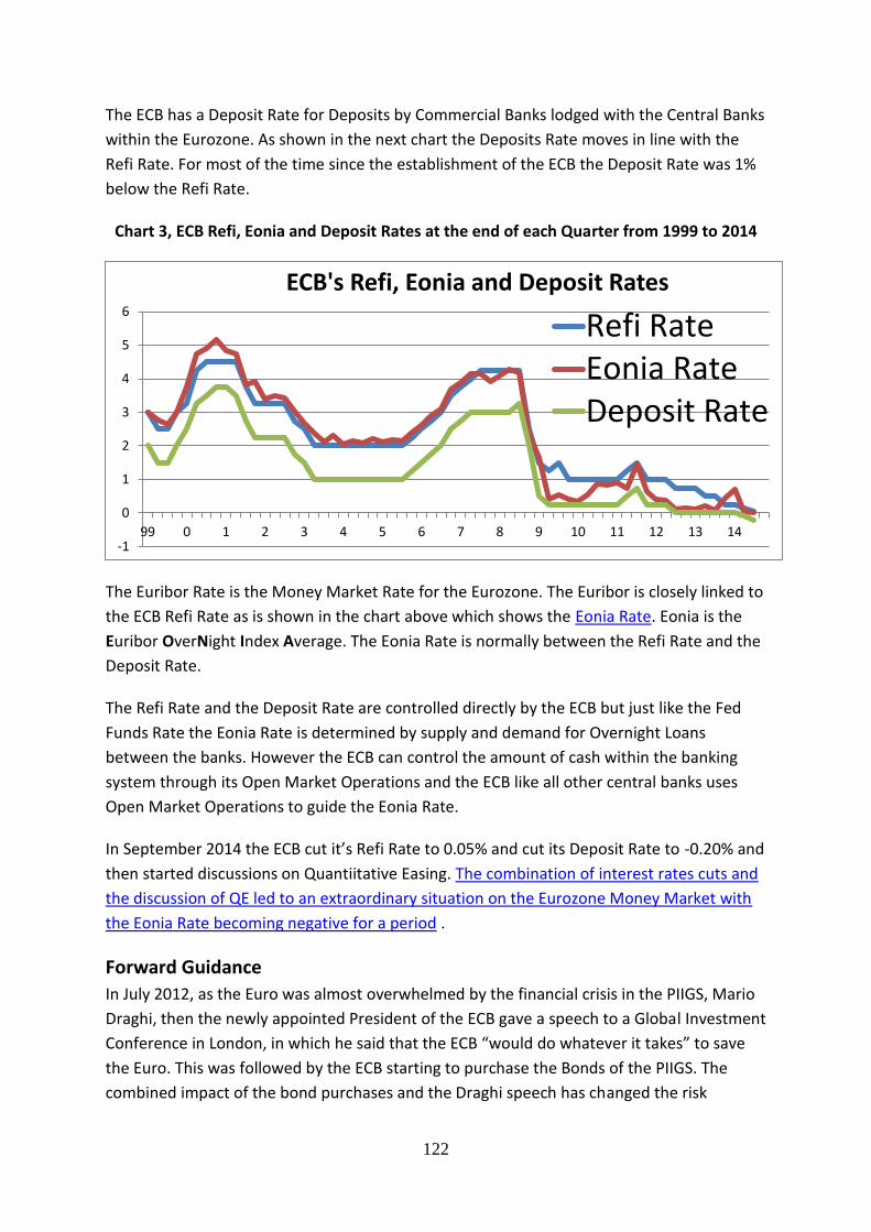
122

The ECB has a Deposit Rate for Deposits by Commercial Banks lodged with the Central Banks

within the Eurozone. As shown in the next chart the Deposits Rate moves in line with the

Refi Rate. For most of the time since the establishment of the ECB the Deposit Rate was 1%

below the Refi Rate.

Chart 3, ECB Refi, Eonia and Deposit Rates at the end of each Quarter from 1999 to 2014

The Euribor Rate is the Money Market Rate for the Eurozone. The Euribor is closely linked to

the ECB Refi Rate as is shown in the chart above which shows the Eonia Rate. Eonia is the

Euribor OverNight Index Average. The Eonia Rate is normally between the Refi Rate and the

Deposit Rate.

The Refi Rate and the Deposit Rate are controlled directly by the ECB but just like the Fed

Funds Rate the Eonia Rate is determined by supply and demand for Overnight Loans

between the banks. However the ECB can control the amount of cash within the banking

system through its Open Market Operations and the ECB like all other central banks uses

Open Market Operations to guide the Eonia Rate.

In September 2014 the ECB cut it’s Refi Rate to 0.05% and cut its Deposit Rate to -0.20% and

then started discussions on Quantiitative Easing. The combination of interest rates cuts and

the discussion of QE led to an extraordinary situation on the Eurozone Money Market with

the Eonia Rate becoming negative for a period .

Forward Guidance

In July 2012, as the Euro was almost overwhelmed by the financial crisis in the PIIGS, Mario

Draghi, then the newly appointed President of the ECB gave a speech to a Global Investment

Conference in London, in which he said that the ECB “would do whatever it takes” to save

the Euro. This was followed by the ECB starting to purchase the Bonds of the PIIGS. The

combined impact of the bond purchases and the Draghi speech has changed the risk

-1

0

1

2

3

4

5

6

99 0 1 2 3 4 5 6 7 8 9 10 11 12 13 14

ECB's Refi, Eonia and Deposit Rates

Refi RateEonia RateDeposit Rate

123

perception on PIIGS Government bonds. This can be seen by looking at Irish 10 year bond

yields over the past 4 years

One of the key powers of a Central Bank is to influence thinking through what is often

referred to as “Forward Guidance”. Forward Guidance involves a central bank giving a clear

indication of the direction of its Monetary Policy into the future. A central bank has

significant control over short term interest rates. The Fed has developed Forward Guidance

into an important policy instrument in the US by, for example, indicating over 2013 and

2014 that it was committed to maintaining a low Fed Funds Rate, at least until 2015. This

reassured medium term lenders and kept medium term interest rates lower. The ECB

started giving Forward Guidance for the first time in July 2013.

In July 2013 the ECB Governing Council announced that it expected the key policy rates to

remain at very low levels for an extended period of time. The Governing Council confirmed

in December 2013 that it continued to expect low interest rates. This forward Guidance had

the impact of keeping medium term interest rates low. In June 2014 the ECB announced

that it would start publishing the minutes of its board meetings from 2015.

For example in September 2014 ECB President Mario Draghi gave an interview on French

radio and said “Interest rates will stay at the present level for an extended period of time

because they can’t go much lower than that”.

Quantitative Easing

The ECB did not follow the lead of the US Fed and the Bank of England in Quantitative

Easing (QE). The German Government and the Bundesbank, with the support of some other

Northern European countries, objected to QE because they believed that this would lead to

inflation.

In September 2012, the ECB in line with Mari Draghi‘s commitment “to do whatever it

takes” to save the Euro, started to purchase the bonds of Eurozone countries, like Ireland,

Greece, Italy, Spain and Portugal which had agreed a fiscal adjustment program with the EU.

The purpose of these bond purchases was to drive up the price of the bonds and reduce the

rate of interest on these government’s bonds. These high bond yields were making it very

difficult for business to raise funds for investment. However these bond purchases were not

Quantitative Easing as the ECB took parallel measures to reduce the money supply by an

equal amount. They called this “Sterilization”.

The ECB policy of keeping interest rate low and purchasing the bonds of countries Southern

European countries had a dramatic effect on Government Bond Yields. This is shown by a

Screen capture of Irish bond yields.

124

Screen capture showing Irish 10 year Bond Yields

The massive reduction in Ireland’s 10 year bond yields (15% in August 2010 to 1.5% in

November 2014) shown in this Chart is not solely due to ECB support as the Irish economy is

now recovering from the financial crisis but the ECB support has contributed to the changed

perception of the risk of Irish bonds.

During 2013 and early 2014 the Eurozone remained in recession and the inflation rate

dropped to 0.5% against a target of 2%. At the same time the value of the Euro increased on

the foreign exchange making Eurozone exports less competitive. This led to a consensus in

the ECB that it should engage in Quantitative Easing. In January 2015 the ECB announced a

program of purchasing Asset-Backed Securities (ABS) starting in March 2015. This QE

Program involves the ECB purchasing €60 billion of Securities each month from March 2015

to September 2016

The prospect of ECB Quantitative Easing, followed by the actual delivery of the QE Program

pushed down the value of the Euro on the FX market in late 2014. This is shown in the Chart

below.

The Euro Exchange Rate

The Euro, as seen above, originated as a European Accounting Unit based on the pre-1971

$US. If the Euro is in effect a European version of the $ then it might be expected that the €

to $ exchange rate would stay close to 1 to 1. The value of the Euro in terms of the $

however has fluctuated massively since 2010 as show by this screen capture from Yahoo.

125

The recent activity of the ECB, involving Quantitative Easing, very low Refi Rate and Forward

Guidance, combined with the Greek Crisis of early 2015, has pushed the € down from $1.38

in early 2014 to $1.12 in May 2015.

The Impact of the Recession on the operation of the Eurozone and ECB

The Euro was set up as a political compromise without the support mechanism needed to

allow a common currency system to function efficiently. The mandate for the ECB was

narrowly focused on keeping inflation low and ignoring the level of economic activity or the

FX value of the currency

It was also a single currency zone without a single system for bank supervision and

resolution.

The impact of the recession on the Eurozone, national finances and the Eurozone banking

system has forced the Eurozone to broaden its focus to take into account economic activity

and the FX value of the currency. It has also driven the Eurozone to develop, effectively, a

banking union to support the monetary union.

The Eurozone is now a well consolidated monetary and banking union with good controls on

both banks and national budgets and a monetary policy which is becoming more flexible

and less focused on inflation prevention.

The ECB's Economia Game allows students to play the Central bank Game.

126

Asset Valuation

Introduction

This note covers the definition of Assets, Art as an Asset, Demand for Assets, supply of

Assets and the market for Assets, Shares or Equities and Property Values including

Commercial Property.

Assets

An Asset is anything that is bought primarily for its ability to generate income and/or capital

gain. An asset is what you invest in. Assets include Government Securities, Shares, Property,

Works of Art, Antiques and Precious metals

There is no clear distinction between Assets and other types of goods such as houses and

machinery. One can visualise a continuum between services and items bought for

immediate consumption and assets bought purely for investment.

Pure Consumption Pure Investment

¦-------------------------------------------------------------------------------------------------------------------¦

Meals out Houses Shares

Personal Services Art Securities

Art as an Asset

Works of art are bought at least partly as investments. These are usually unique items and

are normally sold at auction. The auction price is determined by the bidders and the price

that the under-bidder is prepared to bid. Prices in auctions are therefore to some extent

unpredictable as it only takes two bidders to force the price up. For example in the late

1980s some Japanese businessmen, who were at time among the richest people in the world

because of high asset prices in Japan, developed a craze for European Art. In 1990 Ryeoi

Saito paid $82 million for Vincent van Gogh’s “Portrait of Doctor Gachet” – picture on right.

(The Nikkei Index reached 38,916 in December 1989 and fell to 7,268 in February 2009). In

2006 a painting by Gustav Klimt of “Adele” was sold for $135million – middle picture. The

“Card Players” by Paul Cezanne was sold for $250 million in 2011 – picture on left.

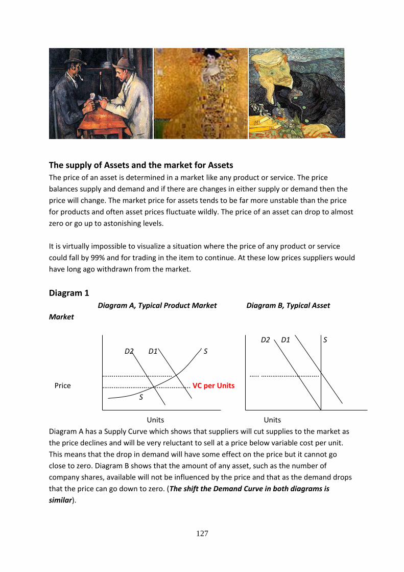
127

The supply of Assets and the market for Assets

The price of an asset is determined in a market like any product or service. The price

balances supply and demand and if there are changes in either supply or demand then the

price will change. The market price for assets tends to be far more unstable than the price

for products and often asset prices fluctuate wildly. The price of an asset can drop to almost

zero or go up to astonishing levels.

It is virtually impossible to visualize a situation where the price of any product or service

could fall by 99% and for trading in the item to continue. At these low prices suppliers would

have long ago withdrawn from the market.

Diagram 1

Diagram A, Typical Product Market Diagram B, Typical Asset

Market

D2 D1 S

D2 D1 S

……..…………………..…… ….. ………………………….

Price ……………………………………….. VC per Units

S

Units Units

Diagram A has a Supply Curve which shows that suppliers will cut supplies to the market as

the price declines and will be very reluctant to sell at a price below variable cost per unit.

This means that the drop in demand will have some effect on the price but it cannot go

close to zero. Diagram B shows that the amount of any asset, such as the number of

company shares, available will not be influenced by the price and that as the demand drops

that the price can go down to zero. (The shift the Demand Curve in both diagrams is

similar).

128

The chart below, from Yahoo Finance, shows the 97% fall in the share price of RBS (Royal

bank of Scotland), one of the biggest banks in the UK. (The price fall in NYSE was from over

$2.00 in 2007 to $0.035 in January 2009, now $0.12). This fall occurred as the RBS had to be

bailed out by the British Government purchasing shares and owning over 80% of the bank.

Before the collapse RBS was for a short period the largest bank in the World in terms of

Assets.

Chart 1

Source, Yahoo Finance

But just as the price of an asset can fall to virtually zero the price can go up to astonishing

levels. This happens when an asset market is dominated by speculation. Speculation refers

to a situation where a product or asset is bought primarily because the price is expected to

rise. The expectation that the price will rise increases demand and fuels what can develop

into a “Speculative Bubble”.

One of the best known examples of a market driven by speculation was the Dutch tulip

market over the period 1631 to 1637. During this period Holland experienced what has been

called “tulip mania” where most of Dutch society started to invest in tulips driving the price

of individual bulbs to astonishing levels. The highest prices were paid for a particular type of

tulip called “Semper Augustus” which had vivid colours and “flaming” as a result of a virus

infection. In February 1637 a single Semper Augustus bulb was sold for 5,200 Guilders or

about 4kg of gold. (The value of 4kg of gold was about $154k in December 2014). The

market collapsed in 1637 bankrupting large numbers of individuals, families and businesses.

The absence of any “floor price” for assets and the potential for a speculative bubble to

develop means that asset prices are often very unstable.

129

Demand for Assets

Since the supply of most assets is largely fixed the market price usually changes as a result

of a change in demand. The Demand for Assets is influenced by four factors:

1) Income or Benefit from the Asset

2) Cost of Holding the Asset

3) Rate of Interest

4) Expectations about changes in the Price of the Asset

Income or Benefit

The income or benefit that an asset generates for the owner is usually a key determinant of

demand for the Asset. This applies to shares, government securities and property. The

relationship between the purchase price of an asset and the income it generates for the

owner is called the Price/Earnings Ratio (P/E Ratio). The purchase price of an asset is usually

between 10 and 25 times the annual income that it generates (P/E Ratio = 10 – 25). If an

asset were to be sold for much less than 10 times the annual income it generates, eg 5

times, it would be so attractive to potential buyers that they would force the price up

through competitive bidding.

The Standard and Poor 500 P/E ratio since 1880 is given below.

Cost of owning the Asset

Some Assets have a holding or ownership cost and other do not and the level of this holding

cost will impact on the price. If an asset has a high holding cost it will deter investors at least

to some degree.

There is no holding cost for Shares or Government Securities but there is a holding cost for

other assets such as Property or Gold. The holding costs for ownership of property are taxes

and maintenance. The State can and does change the taxation situation on property and

thereby changes the value of this property. Owners of large quantities of gold obviously

have to hold it in a secure and expensive location. In times of political or financial instability

however investors usually turn to gold as a safe investment and this drives the price up.

The supply of gold is virtually fixed with annual production, at 2.5k tons, only running at

about 1.5% of the total existing stock of 160k tons.

130

Chart 2, The Price of Gold in $s per Troy Ounce

Source, World Gold Organisation

Gold is not expensive to store and charges are typically 0.2% to 0.3% of the value of the gold

but this is a cost while the gold generates no income. This leads to a situation where in

times of financial and political stability there is a reduced demand for gold but in times of

financial and political instability there is an increased demand and this pushes the price up.

Around 32k tons of gold is held by Monetary Agencies with the US holding over 8k tons and

Germany, France and Italy all holding over 2.5k tons. The IMF holds 2.8k tons. The Central

Bank of Bahrain holds 4.7 tons.

The Rate of Interest

The Rate of Interest has a significant influence on the demand for most Assets. This happens

because investors before making investment decisions usually examine the alternatives

including putting the money into a deposit account in a bank or buying bonds.

In the early 1980s the yield on 10 year US Treasuries reached 14%. Long term bank deposit

rates were similar. Investors in all assets expected to get broadly similar yields and this

drove the prices of these assets lower. In 2012 the yield on these 10 year US Treasuries

went below 2%. This very low yield, accompanied by similar long term deposit rates, drove

investors towards shares and property and the prices of these assets increased rapidly.

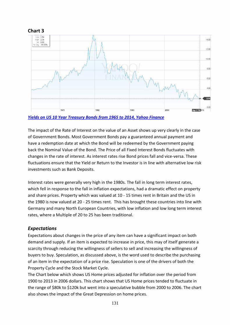
131

Chart 3

Yields on US 10 Year Treasury Bonds from 1965 to 2014, Yahoo Finance

The impact of the Rate of Interest on the value of an Asset shows up very clearly in the case

of Government Bonds. Most Government Bonds pay a guaranteed annual payment and

have a redemption date at which the Bond will be redeemed by the Government paying

back the Nominal Value of the Bond. The Price of all Fixed Interest Bonds fluctuates with

changes in the rate of interest. As interest rates rise Bond prices fall and vice-versa. These

fluctuations ensure that the Yield or Return to the Investor is in line with alternative low risk

investments such as Bank Deposits.

Interest rates were generally very high in the 1980s. The fall in long term interest rates,

which fell in response to the fall in inflation expectations, had a dramatic effect on property

and share prices. Property which was valued at 10 - 15 times rent in Britain and the US in

the 1980 is now valued at 20 - 25 times rent. This has brought these countries into line with

Germany and many North European Countries, with low inflation and low long term interest

rates, where a Multiple of 20 to 25 has been traditional.

Expectations

Expectations about changes in the price of any item can have a significant impact on both

demand and supply. If an item is expected to increase in price, this may of itself generate a

scarcity through reducing the willingness of sellers to sell and increasing the willingness of

buyers to buy. Speculation, as discussed above, is the word used to describe the purchasing

of an item in the expectation of a price rise. Speculation is one of the drivers of both the

Property Cycle and the Stock Market Cycle.

The Chart below which shows US Home prices adjusted for inflation over the period from

1900 to 2013 in 2006 dollars. This chart shows that US Home prices tended to fluctuate in

the range of $80k to $120k but went into a speculative bubble from 2000 to 2006. The chart

also shows the impact of the Great Depression on home prices.

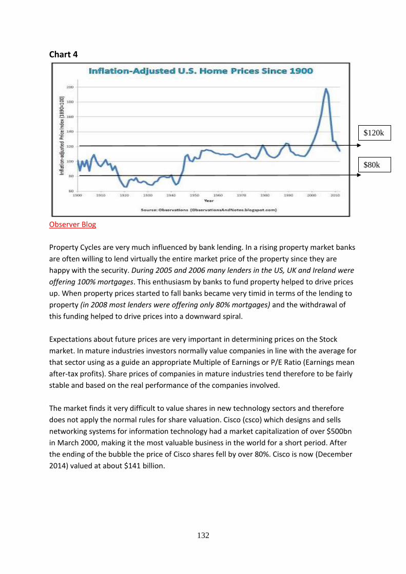
132

Chart 4

Observer Blog

Property Cycles are very much influenced by bank lending. In a rising property market banks

are often willing to lend virtually the entire market price of the property since they are

happy with the security. During 2005 and 2006 many lenders in the US, UK and Ireland were

offering 100% mortgages. This enthusiasm by banks to fund property helped to drive prices

up. When property prices started to fall banks became very timid in terms of the lending to

property (in 2008 most lenders were offering only 80% mortgages) and the withdrawal of

this funding helped to drive prices into a downward spiral.

Expectations about future prices are very important in determining prices on the Stock

market. In mature industries investors normally value companies in line with the average for

that sector using as a guide an appropriate Multiple of Earnings or P/E Ratio (Earnings mean

after-tax profits). Share prices of companies in mature industries tend therefore to be fairly

stable and based on the real performance of the companies involved.

The market finds it very difficult to value shares in new technology sectors and therefore

does not apply the normal rules for share valuation. Cisco (csco) which designs and sells

networking systems for information technology had a market capitalization of over $500bn

in March 2000, making it the most valuable business in the world for a short period. After

the ending of the bubble the price of Cisco shares fell by over 80%. Cisco is now (December

2014) valued at about $141 billion.

$120k

$80k

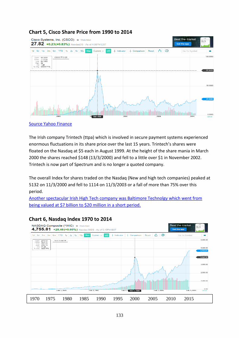
133

Chart 5, Cisco Share Price from 1990 to 2014

Source Yahoo Finance

The Irish company Trintech (ttpa) which is involved in secure payment systems experienced

enormous fluctuations in its share price over the last 15 years. Trintech’s shares were

floated on the Nasdaq at $5 each in August 1999. At the height of the share mania in March

2000 the shares reached $148 (13/3/2000) and fell to a little over $1 in November 2002.

Trintech is now part of Spectrum and is no longer a quoted company.

The overall Index for shares traded on the Nasdaq (New and high tech companies) peaked at

5132 on 11/3/2000 and fell to 1114 on 11/3/2003 or a fall of more than 75% over this

period.

Another spectacular Irish High Tech company was Baltimore Technolgy which went from

being valued at $7 billion to $20 million in a short period.

Chart 6, Nasdaq Index 1970 to 2014

1970 1975 1980 1985 1990 1995 2000 2005 2010 2015

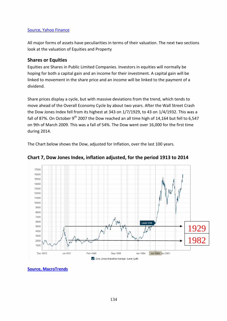
134

Source, Yahoo Finance

All major forms of assets have peculiarities in terms of their valuation. The next two sections

look at the valuation of Equities and Property

Shares or Equities

Equities are Shares in Public Limited Companies. Investors in equities will normally be

hoping for both a capital gain and an income for their investment. A capital gain will be

linked to movement in the share price and an income will be linked to the payment of a

dividend.

Share prices display a cycle, but with massive deviations from the trend, which tends to

move ahead of the Overall Economy Cycle by about two years. After the Wall Street Crash

the Dow Jones Index fell from its highest at 343 on 1/7/1929, to 43 on 1/4/1932. This was a

fall of 87%. On October 9th 2007 the Dow reached an all time high of 14,164 but fell to 6,547

on 9th of March 2009. This was a fall of 54%. The Dow went over 16,000 for the first time

during 2014.

The Chart below shows the Dow, adjusted for Inflation, over the last 100 years.

Chart 7, Dow Jones Index, inflation adjusted, for the period 1913 to 2014

Source, MacroTrends

1929

1982

135

Market Capitalization

Market Capitalization is the total value of the company and is equal to Total Shares Issued *

Price per Share.

The level of a company’s Adjusted Earnings (after-tax profits adjusted for “exceptional

items”) is usually a key determinant of its market value (Market Capitalization). An average

company with average prospects in average times is usually worth about 10 to 15 times its

annual adjusted earnings. The long-run average P/E ratio for the Standard & Poor’s 500

(New York Stock Exchange Index) is about 15. The total value of a company (Market

Capitalization) divided by its annual adjusted earnings is called the P/E Ratio.

Chart 8, The Standard and Poor P/E Ratio for the last 140 years.

Source, Multipl.com

The spike in the P/E Ratio in 2010 can be explained by the drop in company earnings in 2009

and the recovery in investor confidence in 2010 giving low earnings and a high share price

and resulting in a very high P/E Ratio.

The P/E Ratio reflects the "Judgment of the Market" on a Company and its prospects. If the

market judges that the company will be very successful into the future its P/E Ratio will be

high. If the market judges that the company will not be successful into the future its P/E

Ratio will be low. (You cannot use the P/E ratio to judge whether a share offers good value

or not. The P/E ratio is like the length of the queue at a supermarket checkout. If a checkout

is moving fast then many persons will join and it will be a long queue but if the checkout is

moving slowly then few persons will join.

1880 1900 1920 1940 1960 1980 2000

15

10

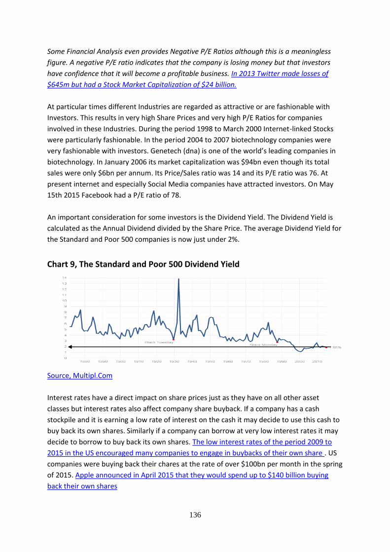
136

Some Financial Analysis even provides Negative P/E Ratios although this is a meaningless

figure. A negative P/E ratio indicates that the company is losing money but that investors

have confidence that it will become a profitable business. In 2013 Twitter made losses of

$645m but had a Stock Market Capitalization of $24 billion.

At particular times different Industries are regarded as attractive or are fashionable with

Investors. This results in very high Share Prices and very high P/E Ratios for companies

involved in these Industries. During the period 1998 to March 2000 Internet-linked Stocks

were particularly fashionable. In the period 2004 to 2007 biotechnology companies were

very fashionable with investors. Genetech (dna) is one of the world’s leading companies in

biotechnology. In January 2006 its market capitalization was $94bn even though its total

sales were only $6bn per annum. Its Price/Sales ratio was 14 and its P/E ratio was 76. At

present internet and especially Social Media companies have attracted investors. On May

15th 2015 Facebook had a P/E ratio of 78.

An important consideration for some investors is the Dividend Yield. The Dividend Yield is

calculated as the Annual Dividend divided by the Share Price. The average Dividend Yield for

the Standard and Poor 500 companies is now just under 2%.

Chart 9, The Standard and Poor 500 Dividend Yield

Source, Multipl.Com

Interest rates have a direct impact on share prices just as they have on all other asset

classes but interest rates also affect company share buyback. If a company has a cash

stockpile and it is earning a low rate of interest on the cash it may decide to use this cash to

buy back its own shares. Similarly if a company can borrow at very low interest rates it may

decide to borrow to buy back its own shares. The low interest rates of the period 2009 to

2015 in the US encouraged many companies to engage in buybacks of their own share . US

companies were buying back their chares at the rate of over $100bn per month in the spring

of 2015. Apple announced in April 2015 that they would spend up to $140 billion buying

back their own shares

137

This was an additional source of demand helping to drive the Dow to over 18,000, its highest

level ever.

Occasionally a number of other factors can influence the value of companies. The value of

companies can be influenced by the level of sales revenue or asset values. During the boom

in internet companies during the early 2000s many companies were valued on the basis of a

multiple of sales revenue. In the take-over of private companies it is quite common for the

business to be valued on the basis of revenue.

Property Values including Commercial Property.

The value of property is determined primarily by Demand and Supply (but the amount of

ground level space, including agricultural land and sites, is fixed). The overall level of

demand for property is mainly determined by the three factors, Population Change,

Prosperity and Interest rates.

Where the population of a region or country is rising this almost inevitably pushes up the

demand for property and a falling population reduces demand. Historically we can see the

impact of population change on property values. After the Black Death of 1348/49 the

population of Europe fell significantly and this led to a fall in property values (and a rise in

the level of wages).

If a country is prosperous this leads to an increase in demand for property and high property

prices. Rapid changes in the level of prosperity will lead to changes in property prices.

The level of interest rates also influences property prices. High interest rates deter investors

in property and so bring property prices down. Low interest rates encourage investment in

property and so drive prices up.

The value of Commercial Property is primarily influenced by rental incomes (linked to

population and prosperity) and the rate of interest. Because there is always only a limited

Supply of attractive Shopping and Business Space combined with High Demand the owners

of this space can rent it out at attractive rents. The Purchase Price will be determined as

follows,

Annual Rent x Multiple = Purchase Price

The Multiple used to value property at any time is very closely related to the Rate of Interest

at that time. The UK and Irish Property Multiple was about 10 in the 1970s and 1980s but

rose to 30 in Ireland for good properties in 2007 at the height of the property boom. For

example the big two Irish banks, AIB and BoI sold bank branches with a leaseback

arrangement for multiples of around 30 during 2006 and 2007. However the financial crisis

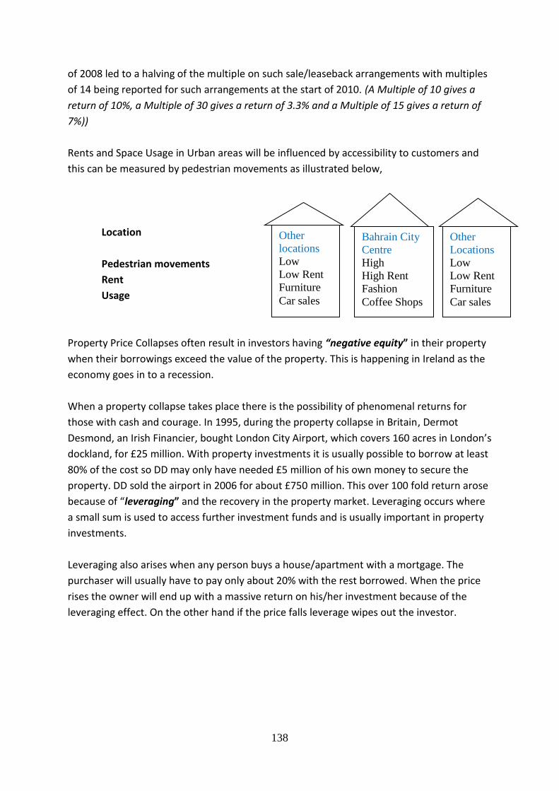
138

of 2008 led to a halving of the multiple on such sale/leaseback arrangements with multiples

of 14 being reported for such arrangements at the start of 2010. (A Multiple of 10 gives a

return of 10%, a Multiple of 30 gives a return of 3.3% and a Multiple of 15 gives a return of

7%))

Rents and Space Usage in Urban areas will be influenced by accessibility to customers and

this can be measured by pedestrian movements as illustrated below,

Location

Pedestrian movements

Rent

Usage

Property Price Collapses often result in investors having “negative equity” in their property

when their borrowings exceed the value of the property. This is happening in Ireland as the

economy goes in to a recession.

When a property collapse takes place there is the possibility of phenomenal returns for

those with cash and courage. In 1995, during the property collapse in Britain, Dermot

Desmond, an Irish Financier, bought London City Airport, which covers 160 acres in London’s

dockland, for £25 million. With property investments it is usually possible to borrow at least

80% of the cost so DD may only have needed £5 million of his own money to secure the

property. DD sold the airport in 2006 for about £750 million. This over 100 fold return arose

because of “leveraging” and the recovery in the property market. Leveraging occurs where

a small sum is used to access further investment funds and is usually important in property

investments.

Leveraging also arises when any person buys a house/apartment with a mortgage. The

purchaser will usually have to pay only about 20% with the rest borrowed. When the price

rises the owner will end up with a massive return on his/her investment because of the

leveraging effect. On the other hand if the price falls leverage wipes out the investor.

Other

locations

Low

Low Rent

Furniture

Car sales

Bahrain City

Centre

High

High Rent

Fashion

Coffee Shops

Other

Locations

Low

Low Rent

Furniture

Car sales

139

Bills, Bonds and Yields Introduction

This note will cover Interest Rates and Yields, Spread of Interest Rates, Market for

Government Bills and Bonds and Yield Curves

Interest Rates and Yields

This note will focus particularly on interest rates and how they impact on Bills and Bonds. A

Bill is effectively a post-dated cheque or a promise to pay a certain amount on a particular

day. Bills originated as Trade Bills and were used to finance trade, particularly British

international trade, up to the 20th century. The purchaser would make out a Bill to the

supplier of goods and pay with the Bill. The Bill was often post-dated for 3 or 6 months

because international trade was slow. The supplier of goods would only accept a guaranteed

Bill so the purchaser would have to get a bank to guarantee the Bill. The supplier of goods

would then go to his bank and get cash. The bank would not pay the “face value” of the Bill

but would discount it, eg if it was a 6 month bill for £100 then the bank might pay £97 for it

and therefore make a return of 6% on its investment. Banks all over England brought Bills to

Discount Houses in London and sold them at a profit. In our example the bank might sell it

for £98. The Discount House, specialized traders in Bills of Exchange, financed their business

by borrowing on the London Money Market at very low rates of interest for short periods.

Most bills are now Government Bills and are referred to as Treasury Bills. Bills are very

useful to banks and other financial institutions as they have a secure return and also know

exactly when they are going to get the cash back. Bills are very useful to governments as

they can borrow at very low rates of interest using bills. Bills are also useful to Central Banks

as they can trade in bills to control the amount of cash within the financial system.

Bonds are promises to pay a certain Rate of Interest over the time period and repay the

amount at a future date (exceptions). The price of a bond will vary with variations in interest

rates. The calculation of the yield, or return on investment, in a bond is often complex

because of interest payments and Capital Gains or Capital Losses. However this complexity

does not arise with a small number of Perpetual Bonds such as the UK 3.5% War Loan. With

this bond the original sum will never be repaid and the owner will continue to receive £3.50

each year for every £100 unit of the bond that she owns.

The Yield is the return on Investment and is linked to the income and the price paid for the

asset

Inverse Relationship between Bond Prices and Interest Rates

The Yield is the return on Investment and is linked to the interest rate adjusted for capital

gain or loss and the price paid for the asset. There is an inverse relationship between bond

prices and yields. This inverse relationship was very easy to show in the case of the UK 3.5%

140

War Loan with the price fluctuating in an inverse relationship to interest rates. The 3.5%

War Loan bond was first issued in 1932 by the British Government to refinance maturing

war bonds from the First World War (1914 – 1918). This bond had no maturity date so the

purchaser of this bond would only get the interest payments. The value of a £100 block of

this bond at any time was £100 *(3.5/Rate of Interest at that time). When the rate of

Interest on very long term UK bonds was 14% the formula gave the value of £100 block as

£100* (3.5/14) = £25). However as interest rates on UK government bonds fell the price of

this bond reached £100 and the UK Chancellor of the Exchequer announced in December

2014 that the UK Government was going to to redeem this security and this security is no

longer traded on the London Stock Exchange.

All bond prices (and bill prices) move in an inverse relationship with interest rates so that

when interest rates rise bond prices fall and when interest rates fall then bond prices rise.

Hargreaves and Lansdown have an excellent website that gives up-to-date prices for UK

bonds.

The Spread of Interest Rates

At any time within any country there will be a significant spread of interest rates. This can

be illustrated by looking at interest rates in Bahrain. The Situation in Bahrain as of May 2014

is as below:

Interest Rate Spread in Bahrain Interest Rate pa

Central Bank of Bahrain Deposit Rate 0.25%

Money Market Rate (3 Months) 0.23%

Three Month Notice Deposits 0.58%

Bahrain Treasury Bills (3 Months) 0.69%

Bahrain Government Bonds 2.0%

Bahrain CB Repo Rate 2.25%

Business Loans (Manufacturing) 3.5%

Personal Loans (Mortgages) 5.7%

Credit Cards 18.7%

Source CBB Bahrain Bank Interest Rates

The entire system of Interest rates tends to move in line with the Money Market Rate and

Central Bank Rate. If Money Market Rates rise or fall then all other interest rates tend to rise

or fall. If (when) the Money Market Rate in Bahrain rises to 4% then all other interest rates

will move up with for example Business Loans to Manufacturing going up to around 7%.

Interest rates for loans vary depending on:

Administrative Costs

Risk of Non-repayment

Risk of Capital Loss, Purchasing Power Loss or FX Loss

141

The admin costs. for Bills and Bonds

Length of the Loan Period

Administration Costs

The administration costs of a loan must be covered by the lending organization. The admin

costs vary massively from the situation on the money market to credit cards. In the Money

Market admin costs are minimal as banks only lend to other banks which they have

complete confidence in. With credit card lending there is a high risk of default and high

admin costs.

Risk of Non-repayment

There is always a risk of non-repayment or “Default”. This note focuses on Government Bills

and Bonds where the risk is lower but here is always some risk. The British Government has

never defaulted on its debt since 1694 but the Greek Government has defaulted 6 times

since 1820. This might indicate that there is no risk in lending to Britain but if Britain had

been defeated in either WW1 or WW2 then it would almost certainly have defaulted. Risk is

measured by Credit Rating Agencies.

The big three credit rating agencies are Standard and Poor (S&P), Moody, and Fitch. All are US

based although Fitch has a dual base in London. S&P and Moody’s are the dominant agencies. The

weaknesses shown up in the Credit Rating System by the Financial Crash of 2008 has led the EU to

consider supporting an EU Credit Rating Agency

Each agency has its own rating system. The rating is based on the agency’s judgment about

the likelihood of Default. The S&P rating system starts with AAA. AAA means that the issuer

is highly unlikely to default as the organization issuing the bond has an “Extremely strong

capacity to meet financial commitments”.

The S&P ratings are:

‘AAA’ — Extremely strong capacity to meet financial commitments. Highest Rating.

‘AA’ — Very strong capacity to meet financial commitments.

‘A’ — Strong capacity to meet financial commitments, but somewhat susceptible to

adverse economic conditions and changes in circumstances.

‘BBB+ — Adequate capacity to meet financial commitments, but more subject to adverse

economic conditions.

‘BBB- — Considered lowest investment grade by market participants.

‘BB+ — Considered highest speculative grade by market participants.

‘BB- — Less vulnerable in the near-term but faces major ongoing uncertainties to adverse

business, financial and economic conditions.

‘B’ — More vulnerable to adverse business, financial and economic conditions but

currently has the capacity to meet financial commitments.

‘CCC’ — Currently vulnerable and dependent on favorable business, financial and

economic conditions to meet financial commitments.

142

‘CC’ — Currently highly vulnerable.

‘C’ — Currently highly vulnerable obligations and other defined circumstances.

‘D’ — Payment default on financial commitments.

There are two broad categories of Bond Grades. These are Investment Grade Bonds and

“Junk Bonds”. Investment Grade Bonds are bonds that carry an S&P rating from AAA to BBB.

“Junk Bond” is a colloquial term for a high-yield bond that carries a rating of 'BB' or lower by

Standard & Poor'. Junk bonds are so called because of their higher default risk in relation to

investment-grade bonds.

There are only 12 countries in the World with an AAA grading from S&P . 10 of these have a

North European culture and the other two are Hong Kong and Singapore. The Major

countries with an AAA rating are Germany, UK, Canada, Australia and Switzerland. The US

has an AA+ rating, Ireland has an A rating Bahrain has a BBB rating. The bonds of a number

of Eurozone countries including Portugal (BB) and Greece (B) are classified as Junk.

The impact of Credit Agency Rating on yields of Government Bonds can be seen within the

Eurozone. The yield on 10 year Government Bonds for a number of Euro Countries, as of

May 2015, is given below. All these countries use the same currency so have the same

Central Bank Interest Rates and very similar inflation rates so the variations in bond yields is

solely based on the perception of risk.

Country S&P Rating Yield on 10 year Government Bonds

Germany AAA 0.6%

France AA 0.9%

Spain BB 1.7%

Greece B 10.9%

Source Bloomberg

The impact of Credit Rating Agency ratings is through influencing demand in the market. In

general investors will be encouraged to buy highly rated bonds and discouraged from buying

lower rated bonds. Some investment funds even have rules that prevent them from

purchasing low rated bonds. However there is not an exact correlation between yields and

agency rating. The situation with Japan illustrates this. Japan does not have an AAA (AA)

rating but its 10 year bond yields, at 0.41%, are the lowest in the world. (US 10 year bonds

were yielding 2.2%). This is because domestic investors make their judgment without taking

credit agency grades

The risk of default has a massive impact on government bond yields. In 2010 and 2011

Ireland went through a period of high default risk as perceived by international investors.

This is shown by the yield on 10 year government bonds. After 2012 the perceived risk

reduced rapidly as a result of actions by the Irish Government to reduce the budget deficit, a

143

recovery in the economy and ECB support. Investors who bought Irish Government Bonds in

2011 made a massive return on their investment.

Irish Government 10 year Bond Yields from 1986 to 2014

Source. tradingeconomics

Risk of Capital Loss, FX loss or Purchasing Power Loss

Capital Loss, or a loss in the value of the asset, will occur if interest rates increase. If

investors believe that the risk of a rise in interest rates is low because there is no inflation

and the financial system is stable then they will be more willing to buy long term bonds.

However if Interest rates are very low and there is inflation then the likelihood is that they

will rise. Capital Loss can be illustrated by the UK 3.5% War Loan .This bond was issued in

£100 blocks in 1932 to repay War Loans from the First World War. It was issued at “par”

which is the nominal value (In the UK the nominal value of a unit is always £100). This

security fell to £50 in the 1960s when interest rates were around 7% and reached an all-

time low of £25 in 1981 when interest rates were around 14%. The 3.5% War Loan reached

£100 in December 2014 when long term interest rates in the UK were 3.5% and at that time

the government bought up the bonds at £100.

The Price of this Bond was very easy to calculate as it moved inversely with the long term

rate of Interest in the UK. Unfortunately for us it is no longer traded so it does not work as

an example.

The fear of Purchasing Power Loss is linked to the Expected Inflation Rate. Japan has a very

low expected inflation rate so lenders are willing to lend to the government at low rates. In

countries where the inflation rate is high the lenders will be reluctant to lend long term at a

rate below the Expected Inflation Rate because they will find other ways of protecting their

wealth. If the expected inflation rate is high then borrowers will be willing to pay high

interest rates because they will realize that their level of repayments will decline in real

terms over time.

The close relationship between 10 year Government Bond Yields and the inflation rate is

shown by the next table. In 6 of the seven major economies the 10 year bond yields are

slightly higher than the rate of inflation. Japan is the exception. It is not the level of Inflation

144

that influences the actions of Lenders and Borrowers but the level of Expected Inflation.

However in most cases the only objective measure of Expected Inflation is Actual Inflation.

In the Japanese situation the inflation rate has been temporarily boosted by a sales tax. This

short term boost in inflation must not have boosted inflation expectations. Also Japanese

investors are not scared by the absence of an AA rating.

10 Year Bond Yields Central Bank Rate Inflation Rate S&P

Ratings

Japan 0.4% 0.1% 2.3% AA

Germany 0.6% 0.05% 0.0% AAA

Canada 1.7% 1.0% 1.2% AAA

UK 1.9% 0.5% 0.0% AAA

US 2.2% 0.25% 0.0% AA+

India 7.9% 7.5% 6.3% BBB-

Over the last 20 years some countries have started issuing inflation protected bonds. The US

started issuing TIPS, Treasury Inflation-Protected Securities, in 1997 and now there are over

$500 billion of these issued. With TIPS the PAR or Nominal value of the Security adjusts to

inflation.

The UK has “Index Linked Bonds” bonds of which this is an example. This particular bond will

mature in 2050 and pays a rate of interest of 0.5% but will be redeemed at an inflation

adjusted value. This bond and all other Index Linked Bonds are linked to the UK Index of

Retail Prices.

The risk or fear of FX loss will also impact on Yields. If a currency is seen as strong on the FX

market then it will reduce the yields on Government Bonds denominated in that currency.

The Euro is seen as a strong currency on the FX markets and this means that bond yields in

the Eurozone are in some cases surprisingly low. As of May 2015 the yield on Irish 10 year

bonds was 1.3% while 10 year UK bond yields was 1.8%. This is the situation even though UK

bonds are seen as very low risk and the UK has an AAA grade from S&P whereas Ireland was

almost bankrupt in 2010 and has an A Grade from S&P.

The fear of Capital Loss, Purchasing Power Loss and FX Loss works through influencing

demand on the market for Bills and Bonds. If the fear of loss is high then it reduces demand

for bonds and as the price of the bonds fall then yields rise. If the fear of loss is low then

demand for bonds will rise pushing up bond prices and pushing down yields.

The Market for Government Bills and Bonds

There is a market for Bills and Bonds just like any other market. The Supply and Demand in

this market is influenced by the price which is in this case the rate of interest. This note will

assume that there is virtually no risk of default so all the analysis below makes that

assumption.

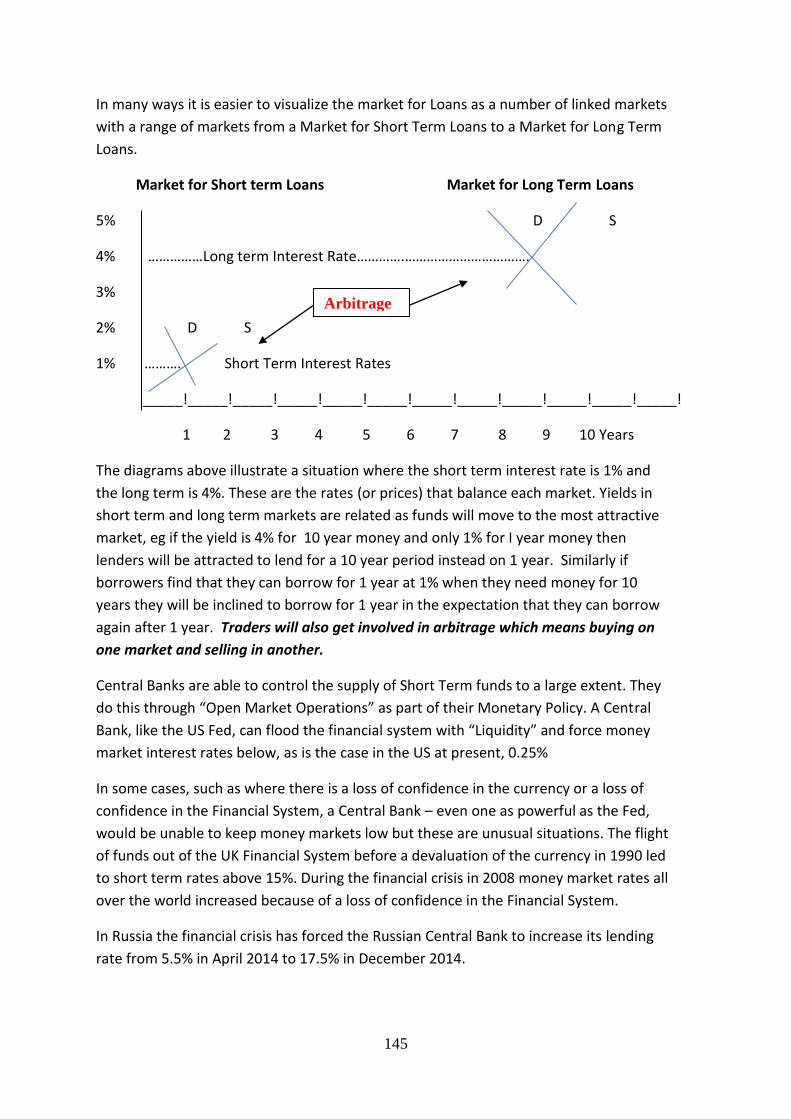
145

In many ways it is easier to visualize the market for Loans as a number of linked markets

with a range of markets from a Market for Short Term Loans to a Market for Long Term

Loans.

Market for Short term Loans Market for Long Term Loans

5% D S

4% ……………Long term Interest Rate………….…………………………….

3%

2% D S

1% ………. Short Term Interest Rates

_____!_____!_____!_____!_____!_____!_____!_____!_____!_____!_____!_____!

1 2 3 4 5 6 7 8 9 10 Years

The diagrams above illustrate a situation where the short term interest rate is 1% and

the long term is 4%. These are the rates (or prices) that balance each market. Yields in

short term and long term markets are related as funds will move to the most attractive

market, eg if the yield is 4% for 10 year money and only 1% for I year money then

lenders will be attracted to lend for a 10 year period instead on 1 year. Similarly if

borrowers find that they can borrow for 1 year at 1% when they need money for 10

years they will be inclined to borrow for 1 year in the expectation that they can borrow

again after 1 year. Traders will also get involved in arbitrage which means buying on

one market and selling in another.

Central Banks are able to control the supply of Short Term funds to a large extent. They

do this through “Open Market Operations” as part of their Monetary Policy. A Central

Bank, like the US Fed, can flood the financial system with “Liquidity” and force money

market interest rates below, as is the case in the US at present, 0.25%

In some cases, such as where there is a loss of confidence in the currency or a loss of

confidence in the Financial System, a Central Bank – even one as powerful as the Fed,

would be unable to keep money markets low but these are unusual situations. The flight

of funds out of the UK Financial System before a devaluation of the currency in 1990 led

to short term rates above 15%. During the financial crisis in 2008 money market rates all

over the world increased because of a loss of confidence in the Financial System.

In Russia the financial crisis has forced the Russian Central Bank to increase its lending

rate from 5.5% in April 2014 to 17.5% in December 2014.

Arbitrage

146

A Central Bank can also force up money market rates as part of monetary policy by

selling Bills and Bonds and draining the financial system of liquidity. If Money Market

rates increase then Long Term Interest Rates will tend to increase. If for example the

money market rate rises from 2% to 5% then a bank is unlikely to be willing to continue

lending below 6%.

In summary, Central Banks have a significant ability to control short term interest rates but

“the market” controls long term rates and this is illustrated by the Diagram below.

.

The Central Bank can flood the money market with Liquidity or drain the money market of

Liquidity very easily and so control short-term rates but the Central Bank cannot control the

price at which investors purchase and sell long term bonds. This has been shown by the

inability of the US Fed to push long term interest rates below 3% for a sustained period.

There is much more volatility in short term than long term interest rates. The Fed was able

to bring down money market rates to virtually zero in 2008 - 2011 but could not drive down

long term rates to the same extent. When the economy recovers the Fed will force up short

term rates but long term will not move up nearly as much.

The Demand for Long-term Loans will be similar to demand for all other types of goods

in that the higher the price the lower the demand and the lower the price the higher the

demand. This can be plotted as a normal demand curve. The supply situation will also be

similar to most markets in that the higher the price the more will be supplied. In the

market for most goods the supply curve becomes very elastic at the level of variable cost

per unit. With long-term loans the situation is very similar as no person will be willing to

lend at a very low rate of interest because the lower the rate of interest the greater the

chance of interest rates rising. A rise in interest rates will mean a capital loss for all

bonds but the level of the loss grows the longer the period of the bond

Range of Short-term and Long-term Bond Yields

15%

12%

9%

6%

3%

Money Market 10 year bonds

147

The supply of Long-term Loans will tend to dry up at around the expected long term

inflation rate and this sets a minimum figure for long-term bonds. Japan has had zero

inflation for the last 10 years and this has led to long-term bond rate below 1%. If the long

term inflation rate is expected to be 2%, as is the case in the US since this is declared Fed

policy, then if interest rates drop below 3% many investors will hold on to cash and keep

their money in bank deposits even with 0% rates on deposits. If inflation is very high, eg

Argentina where inflation is at least 20% pa then persons with savings will want to buy all

kinds of assets or $US to protect their wealth.

Bond investors normally expect that long-term inflation will lead to currency depreciation

and they will want to be compensated for the currency depreciation and inflation by a

higher interest rate. The diagram below illustrates the normal market situation for long-

term government bonds in a low inflation (2%) situation.

8% Demand Supply

6%

4%

2%

A key reason for the unwillingness of lenders to lend long term at low interest rates is the fear of

Capital Loss.

If there is inflation of 2% and interest rates are very low then persons with savings may

decide that the risk of Capital Loss outweighs the benefits from the low level of interest

payment.

Another influence on interest rates is the attractiveness of alternative investments. This

influences Demand. In Japan both property prices and share prices have crashed over the

last 20 years so there is a reluctance to invest either in property or shares. On the other

hand where there is a dynamic economy with rising property and share prices then lenders

will want to charge high interest rates for long term loans and borrowers will be willing to

pay these high interest rates.

Yield Curves

The relationship between the yield (Return on Investment) on Government Bonds and the

length of the Loan is called the Yield Curve. Usually the longer the period of the loan the

higher the Rate of interest. This makes sense as the owner of the money is giving up access

to the money for a longer period and therefore foregoing all opportunities to use this

money in the meantime. Also many investments require a long period before the

Expected Inflation

Rate

148

investment generates profit for the investor so these investors need long term money. This

gives what is called the “Normal Yield Curve”.

The US Treasury Yield Curve for May 2014 below illustrates the Normal Yield Curve.

Source US Treasury

There are three well known Yield Curve Categories, Normal Yield Curves as above, Steeply

Rising Yield Curves and Downward Sloping Yield Curves.

Normal, Steeply Sloping and Downward Sloping Yield Curves

10% ……C…………………………………………………………B………………………………………….

8% …………………………………………………………………………………………………………….

6% ……………………………………………………………………………………………………………..

4% ……………………………………………………A………………………………………………C…...

2% ……B………A……………………………………………………………………………………..……..

Years to Maturity 1 2 3 4 5 6 7 8 9 10 1 12 13 14 15 16 17 18 19

A is a Normal Yield Curve where lenders demand higher interest rates to compensate for the

longer period that they are giving up access to liquidity.B is a Steeply Sloping Yield Curve and

this occurs if short term interest rates are low but there is an expectation of high inflation

and higher interest rates in future.C is a Downward Sloping Yield Curve and this occurs

where short term interest rates are high but there is an expectation of low inflation and low

interest rates in future

Index Linked

Bonds

Traditional

149

US SEC

The US Securities and Exchange Commission is the US Regulator for Financial Investment.

The mission of the SEC “is to protect investors, maintain fair, orderly, and efficient markets,

and facilitate capital formation”. The SEC was set up in 1934 after millions of US investors

had been wiped out in the Wall Street Crash. The SEC was set up to restore investor

confidence in US capital markets by “providing investors and the markets with more reliable

information and clear rules of honest dealing”. The Central bank of Bahrain is the Capital

Markets Regulator for Bahrain. The CCB Capital Markets Supervision Directorate carries out

the same role as the SEC for Bahrain.

150

International Finance

Introduction

International Finance looks at the systems used to pay for goods and services traded across

international boundaries or between currency zones

This note on International Finance will cover International Barter, Silver and Gold Standards,

end of the Gold Standard, Bretton Woods System, Single Gulf Currency, FX Markets and

Purchasing Power Parity Theory.

Barter

It is possible for goods and services to be traded internationally without using currency

through a barter system. International barter was used extensively between communist

countries before 1990. The best known example of this was the Cuban and Soviet Union

barter agreements which involved Cuba supplying the Soviet Union with sugar and the

Soviet Union supplying Cuba with oil.

These barter agreements did not reflect world market prices for the commodities involved.

Both sugar and oil prices fluctuated massively over this period and the barter arrangements

did not reflect the relative values of these commodities on world markets.

Barter arrangements for the international exchange of commodities are feasible though

difficult. However international barter arrangements for branded goods and high tech goods

would be much more difficult to organize.

Silver Standard

Gold and silver as universal currencies were used for international trade before the

emergence of paper money. Up to the 19th century silver coins were dominant. After the

Spanish conquest of South America the massive production of silver coins (The Potosi mine

in Peru produced over 40k tons of silver) led to the Spanish dollar becoming the dominant

currency in international trade for many years.

Gold Standard

The Bank of England however based its paper money on gold. The bank purchased gold

bullion and minted its own coins. The BoE gold coins held exactly ¼ ounce (120 grains) of

pure gold up to from 1604 to 1797. The BoE always redeemed their banknotes with these

gold coins at the rate of one gold coin for a pound. In 1797 during a war with France, there

was a run on the bank and the “convertibility” of the bank’s notes had to be suspended.

Convertibility was re-established in 1821 and lasted until 1914. When convertibility of the £

151

was re-established in 1821 the weight of the new gold coins being minted was 113 grains of

gold and the pound was redeemable in terms of one gold coin per £ so the value of the £

was 113 grains of gold.

During the latter half of the 19th century many countries followed the British practice and

switched their currency base from silver to gold. The US $ originated as a silver coin based

on the “Piece of Eight”, a Spanish silver coin. The piece of eight was a silver coin minted

throughout the Spanish world and called a piece of eight because it was worth 8 Reals. The

value of the Spanish piece of eight was based on the Thaler which was a German coin

containing 1 ounce of silver. During the 19th century the US gradually shifted from silver to

gold as the basis for the currency and in 1900 the US Gold Standard Act laid down the value

of the $ as 23.22 grains of gold.

The British £ was worth 113 grains of gold and the US $ was worth 23.22 grains of gold and

this gave the exchange rate of £ = $4.86.

Parallel with the emergence of the Gold Standard was the general acceptance of Free Trade.

A consensus had emerged that countries were better off adopting British-style Free Trade

Policies and by the start of the 19th century the system for international trade was based on

Free Trade and the system for international finance was based on the Gold Standard.

End of Gold Standard

The Gold Standard System ended in 1914 at the outbreak of World War 1. The outbreak of

the war led to a run on the gold reserves of the Bank of England and it was forced to

suspend the convertibility of the £ in terms of gold. The same situation developed in

Germany, France and many other countries. The US however did not suspend the

convertibility of the $ in terms of gold as US policy makers saw an opportunity for the $ to

replace the £ as the leading international and reserve currency.

During the 1918 to 1945 period there was no agreed international framework for

international trade or international finance. (The League of Nations (predecessor of the

United Nations) had been set up after World War 1 but the US, following a policy called

“Isolationism”, had not joined and, as the US was then the major economic and military

power in the World, its absence left the League much diminished). After World War 1 many

countries tried to go back on to the gold standard but this was not successful

The late 1920s and 1930 also saw a movement away from Free Trade with country after

country introducing restrictions on imports. Herbert Hoover, when running successfully for

US President in 1928, promised to introduce import restrictions to protect US farmers. This

pledge led to the Smooth Hawley Tariff Act of 1930 which imposed tariffs on over 20k

152

different US imports. The Smooth Hawley Act led to retaliation by a large number of

countries including Canada, Britain, France and Germany.

The US maintained the convertibility of the $ in terms of gold into the 1930s but this policy

however had a high price as the Fed was forced on occasion to push up the rate of interest

to protect its gold reserves when the need to stimulate the economy required low interest

rates. The US Government suspended the convertibility of the $ into gold in 1933 and

transferred all the gold reserves of the US banking system to the Federal Reserve Bank. The

US also devalued the $ in 1933 from $20 to $35 per Troy ounce.

Bretton Woods System

At the end of WW2 the Allied Powers (US, UK, France, Soviet Union etc) who defeated

Germany and Japan, reached a number of agreements and set up international institutions

(The United Nations - UN, World Bank, International Monetary Fund - IMF and General

Agreement on Tariffs and Trade – GATT, WTO) to manage international relations after the

War.

One of the most important agreements was reached at a conference in Bretton Woods in

New Hampshire. The Bretton Woods Agreement set up a system of rules, institutions, and

procedures to regulate the international monetary system. The agreement established

the International Monetary Fund ( IMF) and the World Bank.

The Bretton Woods agreement required all signatory countries to maintain a fixed exchange

rate with the US$ while the US maintained a fixed value for the $ in terms of gold at $35 to

Troy ounce. The UK, for example, agreed that the £ would be valued at $4.00.

The Bretton Woods agreement was designed to prevent the competitive devaluations which

had been a feature of the 1930s. Under the Bretton Woods system the value of a currency

could only be changed by agreement. The British devalued the £ a number of times under

This box from the IMF shows the

collapse of international trade in the

1930s as a result of Trade Wars. These

Trade Wars contributed to political

tensions which eventually led to

World War 2 in 1939

One of the achievements of the IMF

and the World Trade Organisation

over the last 6 years was to prevent the

Financial Crisis leading to an outbreak

of Trade Wars as happened in the

1930s.

153

this system with the value of the £ falling from $4.00 to $2.80 in 1949 and from $2.80 to

$2.40 in 1967.

During the 1960s the US imported much more than it exported and this led to a massive

increase in the holdings of $s abroad. By the late 1960s the US only had gold reserves of

about 30% of the value of international holdings of $s. A combination of problems

developed in the US in 1971 including the “Impeachment” of President Nixon. Germany was

unwilling to revalue their currency which the US felt was undervalued. Switzerland and

France started converting their $ reserves into gold and there was a likelihood that many

other countries would follow suit. The United States unilaterally ended the convertibility of

the US dollar to gold in 1971. The ending of the convertibility of the $ brought the Bretton

Woods System to an end.

The major currencies, such as the £ then adopted floating exchange rate policies with the

value of the currency being solely determined by buying and selling on the foreign exchange

market. The £ fluctuated wildly over the period 1971 to 1975 relative to the $ at one stage

falling to $1.20 and another rising to $2.60.

After the ending of the Bretton Woods system a number of different exchange rate policies

were adopted by countries. The European Union developed the Euro which now has 19

member countries using the single currency. Britain joined the European Monetary System,

a precursor for the Euro, in 1989 but left in 1991.

Saudi Arabia and Bahrain linked their currencies to the $ in 1980. Both Saudi Arabia and

Bahrain depend on oil export for their foreign exchange earnings and oil is priced in $s. The

Central Bank of Bahrain justifies its exchange rate policy as follows “Bahrain is a small open

economy for which external trade, i.e. exports and imports, corresponds to more than 140%

of GDP. It is therefore important to have a monetary arrangement which mirrors that of

major trading partners. The Bahraini dinar is pegged to the US dollar. The peg has been

effectively unchanged since 1980. The use of a large foreign currency as a nominal anchor

for monetary policy is a frequent arrangement among small open economies and has proven

to be successful if supported by appropriate fiscal and structural policies. The US dollar peg

serves to enhance credibility and transparency of monetary policy to maintain financial

stability”.

A fixed exchange rate requires that a central bank or other monetary agency is willing to buy

and sell the country’s currency at the fixed rate in terms of the base currency. In the case of

Bahrain the Central Bank of Bahrain “maintains an exchange rate peg at 0.376 Bahraini

dinars to the US dollar” and “The CBB offers a foreign exchange facility, implying that it

stands ready to buy and sell US dollars, at rates very close to the official exchange rate. The

CBB provides this facility to commercial banks located in the Kingdom of Bahrain”.

The CBB has to ensure that it is always able to meet the demand for $s. The CBB therefore

maintains part of its foreign reserves as $ deposits with commercial banks, both inside and

outside Bahrain. The reserves also consist of short, medium and long term debt securities of

154

high credit standards, such as US Treasury bills and bonds, euro bonds, mortgage backed

securities, asset-backed securities and corporate bonds.

According to Article 19 of the Central Bank of Bahrain and Financial Institutions Law, foreign

reserves permanently maintained by the Central Bank shall not be less than 100% of the

value of the currency in circulation. At the end of 2011, which is the most recent year for

which the CBB Annual Report is available, the total value of BD in circulation was 500 million

and the total foreign reserves of the CBB was over BD2 billion.

Single Gulf Currency

In 1981 Saudi Arabia, Kuwait, Bahrain, Qatar, UAE and Oman set up the Gulf Cooperation

Council, GCC. The GCC agreement committed the countries to cooperate in security,

economic and monetary affairs. The countries committed themselves to the establishment

of a common currency by 2010 but this has not been achieved. All the countries involved,

apart from Kuwait, have had stable relationships between their currencies since the 1980s

because all are pegged to the $. The Kuwait currency is pegged to a basket of currencies.

The early success of the Euro encouraged the countries involved to move forward but the

crisis in the Euro after the world recession has changed thinking.

Kuwait pegged its currency (Kuwait Dinar) to a basket of currencies from 1975 to 2002 and

then linked its currency to the $ at KD = $3.45 but reverted to an “undisclosed weighted

basket” in 2007. This was because they were unhappy with the decline in the value of the $

on the foreign exchange market.

In 2010 Saudi, Bahrain, Qatar and Kuwait signed a Monetary Union Agreement to establish a

single gulf currency and as step towards that to set up a Gulf Monetary Council based in

Riyadh. The role of the Gulf Monetary Council is to prepare for the setting up of the new

currency and the new central bank.

The Foreign Exchange (FX) Market

The foreign exchange market (FX) is like all markets with the price (the FX rate) determined

by Supply and Demand. The Bank for International Settlements carries out a survey of the

FX markets every three years. This is the best information source on FX markets .

The major sources of supply and demand for a currency on the FX market are linked to:

Trade, Travel and Tourism,

Long-term Capital Movements,

Hot Money and

Speculation.

155

Most foreign exchange demand and supply arises through the normal activities of

international trade, international travel or international tourism. When a person or business

normally resident in any country wants to purchase goods or services from abroad they

must sell their local currency to purchase the currency of the seller or else they pay in their

local currency and the seller of the goods and services sells their currency. All imports of

goods and services lead to a foreign exchange outflow and this is normally balanced by a

foreign exchange inflow from the export of goods and services.

Long term investment also creates supply and demand on the foreign exchange market. An

investor into any country will normally have to buy the local currency to make the

investment. Long-term investments therefore create inflows and outflows of foreign

currency.

Some investors move money from one currency to another depending on the rates of

interest available in that currency. This is often described as “hot money”. High interest

rates attract hot money and low interest rates deter hot money flows. The very low interest

rates in the US after 2008 discouraged investors from purchasing $s and made the € more

attractive but the speculation in late 2014 the ECB decision to keep its interest rates and

engage in Quantitative Easing led to the € falling from $1.40 in May 2014 to $1.10 in May

2015.

The final source of supply and demand is linked to speculation. If a currency is perceived by

investors as weak and therefore likely to be devalued then this will lead to a rush to sell.

Persons with cash or deposits will try to exchange the currency that is perceived as weak for

strong currencies. Speculators will also borrow the weak currency to sell it. This will

inevitably lead to an increase in short term interest rates in the weak currency. The

speculative activity that forced the UK out of the European Monetary System in 1991 is well

known.

The Russian Central Bank was forced to increase its lending rate by to 17.5% to support the

currency on the FX market in late 2014. The collapse of the Ruble was triggered by US and

EU sanctions against Russia linked to events in Ukraine and the fall in the price of oil. The

Russian Central Bank was forced to intervene in the FX market and did so by increasing

interest rates and using its foreign exchange reserves to purchase Rubles. This has led to a

recovery in the value of the Ruble from a low of $ = 63 Rubles to $ = 56 Rubles on

22/12/2014. The fall in the Ruble value on the FX markets is illustrated by the next chart

from Yahoo Finance.

156

US$ to Russian Ruble Exchange Rate from October 2014 to December 2014

Source, Yahoo Finance=

This chart show that the value of the Ruble fell from around $40 Ruble to $ in October to

almost 66 Ruble to the $ in mid December before recovering to 56 Ruble to $ at 22/12/14.

Speculation is linked to the level of confidence in a currency. During 2010, 2012 and 2014

the Eurozone went through three crises which undermined confidence in the currency.

Each of these crisis was associated with a drop in the value of the €. The screenshot below,

from Yahoo Finance, shows the variation in the $/€ exchange rate over the last 5 years and

the three low points for the value of the Euro are clear.

€/$ Exchange Rate over the last 5 years

Source, Yahoo Finance

157

Purchasing Power Parity Theory

The theory of Exchange Rates states that at the existing Exchange Rates an equivalent sum

should buy the same quantity of goods and services in all countries. This theory implies a

direct connection between inflation and changes in the exchange rate. The theory is largely

supported by the experience since 1945.

Over that period some countries, including the UK, have had significant inflation and other

countries, including Germany had very little inflation. The differences in inflation rates have

largely been reflected in the Exchange Rates with the value of currencies, where there was

inflation constantly falling against the currencies which had little inflation.

The Euro was established in 1971 (Then called the European Unit of Account) as a European

version of the $ and had a value of one 1970 $.

The Chart below shows the US and German Inflation Rates, as measured by the Consumer

Price Index, over the period 1971 to 2003.

US and German Inflation from 1971 to 20014

Over the 43 years from 1971 to 2014 the level of inflation in Germany has been below that

of the US for 37 years and the average inflation rate in Germany over that period was 2.9%

compared with 4.3% for the US. Germany is the dominant economy within the Eurozone

and the change in the $/€ exchange rate reflects the difference in the inflation rate between

the two countries.

Competitiveness and the FX Rate

It is often very difficult to determine what is the correct FX rate for a currency but it is

usually very easy to determine if the FX rate is too high. If the FX value of a currency is too

-2

0

2

4

6

8

10

12

14

16

1971 1980 1990 2000 2010

Germany US

158

high then it will be very difficult to export goods and services so exports will fall. Exports

generate demand for the country’s currency on the FX market. If the FX value of a currency

is too high it will also make it very easy for foreign business to sell goods and services in the

country. Imports generate a supply of the country’s currency on the FX market.

Supply and Demand on the FX Market

D S

FX Price Too High ………………………………

FX Price Correct

FX Price Too Low …………………………….

Volume

Competitiveness however is a very complex issue. Competitiveness does not just take into

account the level of costs. A country can be highly competitive even with high cost if the

products and services sold by the country are such high quality and high tech that they

command high prices. Switzerland is an example of a high cost but highly competitive

country because the items produced in Switzerland command high prices. An example of

this is the Swiss Textile Industry. In the 19th century Switzerland produced textile products

but the industry transitioned from producing textile products to producing high quality

textile machinery that dominates the world market in many sectors.

If a country loses competitiveness through its costs rising too much, without compensating

improvements in quality and technology levels, what will happen is that exports will fall and

imports will rise and the increased supply and reduced demand for the currency on the FX

market will change the FX rate.

The Economist Magazine produces each year an index of the value of currencies based on

the price of a McDonald’s Big Mac. They calculate in US dollars the price of the Big Mac in

various countries and compare that with the US price of the Big Mac. Based on this the

Economist Magazine works out whether a currency is over-valued or undervalued. The

Economist Big Mac Index does not cover the Bahrain Dinar but does cover over 40

currencies. The average price of the Big Mac in the US in January 2014 was $4.63. The

average price for the Big Mac in the Eurozone was €3.66 which at the going exchange rate

was $4.96. This implied that the € was 7% overvalued in January 2014. If the Big Mac Index

was correct the value of the Euro should have fallen from $1.37 in January 2014 to about

$1.27 now but the actual exchange rate now, May 2015 is around $1.10.