Non-parametric estimation of a timevarying GARCH model

by Neelabh Rohan and T. V. Ramanathan

Technical Report 3/2011

Department of Statistics and Centre for Advanced StudiesUniversity of Pune, 411 007, INDIA

May, 2012 (Revised)

1

Non-parametric estimation of a timevarying GARCH model

Neelabh Rohan1 and T. V. Ramanathan2

Department of Statistics and Centre for Advanced StudiesUniversity of Pune, 411 007, INDIA

Abstract

In this paper, a non-stationary time-varying GARCH (tvGARCH) model has beenintroduced by allowing the parameters of a stationary GARCH model to vary as functionsof time. It is shown that the tvGARCH process is locally stationary in the sense that itcan be locally approximated by stationary GARCH processes at fixed time points. Wedevelop a two step local polynomial procedure for the estimation of the parameter func-tions of the proposed model. Several asymptotic properties of the estimators have beenestablished including the asymptotic optimality. It has been found that the tvGARCHmodel performs better than many of the standard GARCH models for various real datasets.

Mathematical Subject classification: 62M10, 62G05

Keywords: Local polynomial estimation, time-varying GARCH, volatility modelling.

1Corresponding author Email: neelabh.stats@yahoo.co.in2Email: ram@stats.unipune.ac.in

2

1 Introduction

The first decade of the 21st century left the global economies grappling with the conse-

quences of the financial crisis followed by an uninvited rash of currency wars. Many of

the emerging economies started receiving large capital inflows that have the potential to

destabilizing the economy. Perhaps, the most deleterious consequence of capital inflows

has been the strengthening of domestic currency, which can lead to a loss in export com-

petitiveness. This, in turn led to currency wars-the phenomenon of several emerging and

developed countries intervening in currency market simultaneously in order to ensure that

their currency will not be the only one that appreciates. Such a phenomenon may induce

instability and hence non-stationarity in the bilateral exchange rate volatility process,

implying the failure of standard stationary volatility models. In this paper, we address

this problem by considering a GARCH model with time varying parameters.

Non-stationary volatility models have got considerable attention recently, see for ex-

ample Mercurio and Spokoiny (2004), Mikosch and Starica (2004), Starica and Granger

(2005), Dahlhaus and Subba Rao (2006), Amado and Terasvirta (2008), Fryzlewicz, Sap-

atinas and Subba Rao (2008) and Chen and Hong (2009) and among others. Dahlhaus

and Subba Rao (2006) proposed a time-varying ARCH (tvARCH) model for the volatil-

ity process by allowing the parameters of a stationary ARCH model to change slowly

through time. Fryzlewicz et al. (2008) developed a least-squares estimation procedure

for such a tvARCH model. We generalize the tvARCH model introduced by Dahlhaus

and Subba Rao (2006) to time varying GARCH (tvGARCH) by allowing the parameters

of a stationary GARCH model to vary as functions of time.

Dahlhaus and Subba Rao (2006) showed that the tvARCH model can be approxi-

mated by stationary ARCH processes locally. We extend their results to the tvGARCH

model and show that a non-stationary tvGARCH process can be locally approximated by

stationary processes at specific time points. Therefore, the tvGARCH model is asymp-

totically locally stationary at every point of observation, but it is globally non-stationary

because of time-varying parameters. Such an approximation further helps us in deriving

the asymptotic distribution of the estimators.

An alternative approach to incorporate non-stationarity in the volatility process is the

varying coefficient GARCH model (see Cizek and Spkoiny (2009) and references therein).

The estimation of a varying coefficient GARCH model requires the search for local time

3

intervals of homogeneity over the entire period, such that the parameters of the process

remain nearly a constant over each interval. The estimation is carried out using the

quasi-maximum likelihood (QML) approach. However, the QML procedure is not very

reliable when the sample size is small, since the quasi-likelihood tends to be shallow about

the minimum for small sample sizes, see Shephard (1996), Bose and Mukherjee (2003)

and Fryzlewicz et al. (2008). In addition, the QML estimator does not admit a closed

form solution. The model and estimation procedure of Amado and Terasvirta (2008) also

suffers from similar drawbacks.

We develop a two-step local polynomial estimation procedure for the estimation of the

proposed tvGARCH model. One can refer to Wand and Jones (1995), Fan and Gijbels

(1996) and Fan and Zhang (1999) among others for the application of local polynomial

techniques in various regression models. The proposed two-step estimation procedure

requires the estimation of a tvARCH model initially in the first step. In the second step,

we obtain the estimator of the tvGARCH model using the initial estimator. Expressions

for the asymptotic bias and variance of the estimators in both the steps are derived and

asymptotic normality is established. It is found that the asymptotic MSE of estimators

of the parameter functions of tvGARCH model remain invariable for a wide range of the

initial step bandwidths, thus making it computation friendly. Moreover, our estimator

achieves the optimal rate of convergence under a higher order differentiability assumption

of the parameter functions.

Even though this paper deals with tvGARCH (1,1) process only, the results presented

here can be extended to a general tvGARCH (p, q) with appropriate modifications. In

the empirical analysis of financial data, lower order GARCH (1,1) model has often been

found appropriate to account for the conditional heteroscedasticity. It usually describes

the dynamics of conditional variance of many economic time series quite well, see for

example Palm (1996). Therefore, in this paper we concentrate on tvGARCH (1,1) model.

We illustrate the performance of the tvGARCH model using various bilateral ex-

change rate and stock indices data in the past decade. The tvGARCH model is shown

to outperform several stationary GARCH as well as tvARCH models in terms of both

in-sample and out of sample prediction. The model is also found to be performing better

than a long memory model in predicting the volatility.

The rest of the paper is organized as follows. A tvGARCH model and its properties

4

have been discussed in Section 2. Section 3 develops a two step local polynomial estima-

tion procedure for the model. We establish the asymptotic properties of the estimators

in Section 4. Several applications of the tvGARCH model are given in Section 5. All the

proofs are deferred to the Appendix.

2 A time varying GARCH model

Let ǫt be a process such that E(ǫt|Ft−1) = 0 and E(ǫ2t |Ft−1) = σ2

t , where Ft−1 =

σ(ǫt−1, ǫt−2, . . .). Suppose vt is a sequence, independent of ǫt, of real valued indepen-

dent and identically distributed random variables, having mean 0 and variance 1. Then

a GARCH model with time varying parameters is defined as

ǫt = σtvt,σ2

t = ω(t) + α(t)ǫ2t−1 + β(t)σ2

t−1

(1)

where ω(·), α(·) and β(·) are certain non-negative functions of time.

In order to obtain a meaningful asymptotic theory, we rescale the domain of the

parameter functions of (1) to unit interval. That is, we study the following process,

ǫt = σtvt,

σ2t = ω

(tn

)+ α

(tn

)ǫ2t−1 + β

(tn

)σ2

t−1, t = 1, 2, . . . , n.(2)

The sequence of stochastic processes ǫt, t = 1, 2, . . . , n is said to follow a tvGARCH

process if it satisfies (2). Here ω(u), α(u), β(u) ≥ 0 ∀ u ∈ (0, 1] ensure the non-negativity

of σ2t . We define ω(u), α(u), β(u) = 0 for u < 0. Such a rescaling is a common technique in

non-parametric regression and it does not affect the estimation procedure, see Dahlhaus

and Subba Rao (2006).

Now we show that the tvGARCH process can be locally approximated by stationary

GARCH processes at specific time points. This allows us to refer the tvGARCH as a lo-

cally stationary process. Towards this, first we state the following technical assumptions:

Assumption 1. (i) There exists δ > 0 such that

0 < α(u) + β(u) ≤ 1 − δ, ∀ 0 < u ≤ 1 and supu

ω(u) < ∞.

(ii) There exist finite constants M1,M2 and M3 such that ∀ u1, u2 ∈ (0, 1],

|ω(u1) − ω(u2)| ≤ M1|u1 − u2||α(u1) − α(u2)| ≤ M2|u1 − u2||β(u1) − β(u2)| ≤ M3|u1 − u2|.

5

The Assumption 1 (i) here is similar in spirit to the stationarity condition for GARCH

(1,1) model discussed by Nelson (1991). This condition is required for the existence

of a well defined unique solution to the tvGARCH process. It is also sufficient for the

tvGARCH to be a short memory process. The Lipschitz continuity condition for the

parameters in Assumption 1 (ii) is required for the local stationarity of the tvGARCH

process. Similar condition is also assumed by Dahlhaus and Subba Rao (2006) for pa-

rameters of the tvARCH process. Notice that we do not make any assumption on the

density function of ǫt. Therefore, the methodology introduced in the paper will be useful

for analyzing data with heavy tailed distributions which is a common phenomenon in

financial time series.

Before proceeding further, we show in Proposition 2.1 that the tvGARCH process

possesses a well defined unique solution. In the Proposition 2.2, we derive the covariance

structure of the tvGARCH process and show that tvGARCH is a short memory process.

Proposition 2.1. Let the Assumption 1 (i) hold. Then the variance process (2) has

a well defined unique solution given by

σ2t = ω

(tn

)+

∞∑i=1

i∏j=1

(α(

t−j+1n

)v2

t−j + β(

t−j+1n

))ω(

t−in

),

such that |σ2t − σ2

t | → 0 a.s., if σ20 (starting point) is finite with probability one. Also,

infu

ω(u)/(1 − infu

β(u)) ≤ σ2t < ∞ ∀ t a.s.

Proposition 2.2. Suppose that the Assumption 1 (i) is satisfied for the tvGARCH

process. Further assume that E|vt|4 < ∞. Then for a fixed k ≥ 0 and 0 < δ < 1,

Cov(ǫ2t , ǫ

2t+k) = O

((1 − δ)k

).

Now we define a stationary GARCH (1,1) process, which locally approximates the original

process (2) in the neighborhood of a fixed point (see Proposition 2.3). Let ǫt(u0), u0 ∈(0, 1] be a process with E(ǫt(u0)|Ft−1) = 0 and E(ǫ2

t (u0)|Ft−1) = σ2t (u0) where Ft−1 =

σ(ǫt−1, ǫt−2, . . .). Then ǫt(u0) is said to follow a stationary GARCH process associated

with (2) at time point u0 if it satisfies,

ǫt(u0) = σt(u0)vt,σ2

t (u0) = ω(u0) + α(u0)ǫ2t−1(u0) + β(u0)σ

2t−1(u0).

(3)

6

Under Assumption 1(i), (3) is a stationary ergodic process. It is also sufficient for ǫt(u0)

to be weakly stationary. A unique stationary ergodic solution to (3) is

σ2t (u0) = ω (u0) +

∞∑i=1

i∏j=1

(α (u0) v2

t−j + β (u0))ω (u0) . (4)

Here |σ2t (u0) − σ2

t (u0)| → 0 a.s. (see Nelson (1991)). Now in the following proposition,

we show that if the time point (t/n) is close to u0, then (3) can be locally considered as

an approximation to (2).

Proposition 2.3. Suppose that the Assumptions 1 (i) and (ii) are satisfied, then the

process ǫ2t can be approximated locally by a stationary ergodic process ǫ2

t (u0). That

is, there exists a well defined stationary ergodic process Vt independent of u0 and a con-

stant Q < ∞ such that

|ǫ2t − ǫ2

t (u0)| ≤ Q(∣∣∣ t

n− u0

∣∣∣+ 1n

)Vt a.s.

or equivalently

ǫ2t = ǫ2

t + OP

(∣∣∣ tn− u0

∣∣∣+ 1n

).

We can also write (2) by recursive substitution,

σ2t = α0(

tn) +

t−1∑k=1

αk(tn)ǫ2

t−k + σ20

t∏i=1

β(

t−i+1n

), (5)

where

α0(tn) = ω

(tn

)+

t−1∑k=1

ω(

t−kn

) k∏i=1

β(

t−i+1n

), αk(

tn) = α

(t−k+1

n

) k−1∏i=1

β(

t−i+1n

),

k = 1, 2, . . . t − 1.

Here we take0∏

i=1β(

t−i+1n

)= 1. Notice that the functions αk(·) here are geometrically

decaying as k → ∞ under Assumption 1(i). Also, if σ20 is finite with probability one, then

σ20

t∏i=1

β(

t−i+1n

)P→ 0 as t → ∞, n → ∞. Here,

P→ denotes convergence in probability.

3 Local polynomial estimation

The local polynomial estimation of the tvGARCH model (2) can be carried out in two

steps. In Step 1, we obtain a preliminary estimate of σ2t using a time varying ARCH

(p) model, exploiting the representation (5) of tvGARCH. In the second step, we finally

7

reach the estimators of the parameter functions of tvGARCH. It has been shown that

with appropriately chosen bandwidth, the rate of convergence of the MSE of final esti-

mates become independent of the initial step estimates.

Step 1. First, we obtain a preliminary estimate of σ2t using the following tvARCH

(p) model;

σ2t = α0(

tn) + α1(

tn)ǫ2

t−1 . . . + αp(tn)ǫ2

t−p

which can also be written as

ǫ2t = α0(

tn) + α1(

tn)ǫ2

t−1 . . . + αp(tn)ǫ2

t−p + σ2t (v

2t − 1).

Here, p is such that p = pn → ∞ as n → ∞. Among several choices of such a p, one

specific choice is log n. The asymptotic results derived in Section 4 for the tvGARCH

model hold for pn → ∞. However, we drop the suffix n for notational simplicity. We

use local polynomial technique to estimate the functions αi(u), i = 0, 1, . . . p, treating

σ2t (v

2t −1) as error. Now onwards, we will denote (t/n) = ut. We assume that the function

αi(·) possesses a bounded continuous derivative up to order d + 1, (d ≥ 1) (see Section

4). Using Taylor’s series expansion, the function αi(u) can locally be approximated in

the neighborhood of a point u0 by,

αi(ut) ≈ αi0 + αi1(ut − u0) + . . . + αid(ut − u0)d, i = 0, 1, . . . , p

where αij, j = 0, 1, . . . d are constants. Therefore, given a Kernel function K(·), we get

the estimator by minimizing,

L =n∑

i=p+1

(ǫ2i −

d∑k=0

(α0k +p∑

j=1αjkǫ

2i−j)(ui − u0)

k

)2

Kh1(ui − u0) (6)

where Kh1(·) = (1/h1)K(·/h1) and h1 denotes the bandwidth. Define

Ut = [1, (ut − u0), . . . , (ut − u0)d]1×(d+1) t = 1, 2, . . . , n ,

X1 =

Up+1 ǫ2pUp+1 . . . ǫ2

1Up+1

Up+2 ǫ2p+1Up+2 . . . ǫ2

2Up+2...

.... . .

...Un ǫ2

n−1Un . . . ǫ2n−pUn

,

W1 = diag(Kh1(up+1 − u0), . . . , Kh1(un − u0)) and Y1 = [ǫ2p+1, . . . ǫ

2n]⊤.

8

The estimator of αi(u0) as a solution to least-squares problem (6) can be expressed as,

αi(u0) = e⊤i(d+1)+1,(p+1)(d+1)(X⊤1 W1X1)

−1X⊤1 W1Y1, i = 0, 1, . . . , p. (7)

Here and throughout the paper, we use the notation ek,m for a column vector of length

m with 1 at kth position and 0 elsewhere. Therefore, an initial estimate of σ2t is obtained

by,

σ2t = α0(ut) +

p∑k=1

αk(ut)ǫ2t−k,

where α0(ut) and αk(ut) represent the estimators of α0(ut) and αk(ut) respectively. They

are calculated using (7) at ut. We set ǫ2t = 0, ∀ t ≤ 0 for the practical implementation.

This method can also be used for the estimation of a tvARCH (p) model of Dahlhaus

and Subba Rao (2006).

Step 2. In this step, we use the conditional variance initially estimated in Step 1 to

get the estimates of the parameter functions of tvGARCH process. The parameter func-

tions ω(·), α(·) and β(·) are assumed to be continuously differentiable up to order d + 1.

Using Taylor’s series expansion, we can write,

ω(ut) ≈ ω02 + ω12(ut − u0) + . . . + ωd2(ut − u0)d

α(ut) ≈ a02 + a12(ut − u0) + . . . + ad2(ut − u0)d

β(ut) ≈ b02 + b12(ut − u0) + . . . + bd2(ut − u0)d

where ωi2, ai2 and bi2, i = 0, 1, . . . , d are constants. We can write (2) as

ǫ2t = ω( t

n) + α( t

n)ǫ2

t−1 + β( tn)σ2

t−1 − β( tn)(σ2

t−1 − σ2t−1) + σ2

t (v2t − 1). (8)

Corollary 2 (in Section 4) shows that for a particular choice of the Step 1 bandwidth

h1 = o(h2), E(σ2t−1 − σ2

t−1) is asymptotically negligible. Here h2 denotes the bandwidth

in the Step 2. The estimates are obtained by minimizing

L =n∑

i=2

(ǫ2i −

d∑k=0

(ωk2 + ak2ǫ2i−1 + bk2σ

2i−1)(ui − u0)

k

)2

Kh2(ui − u0).

Define

X2 =

U2 ǫ21U2 σ2

1U2

U3 ǫ22U3 σ2

2U3...

......

Un ǫ2n−1Un σ2

n−1Un

,

W2 = diag(Kh2(u2 − u0), . . . , Kh2(un − u0)), and Y2 = [ǫ22, . . . , ǫ

2n]⊤.

9

Then, the exact expressions for the estimators are given by

ω(u0) = e⊤1,3(d+1)(X⊤2 W2X2)

−1X⊤2 W2Y2,

α(u0) = e⊤d+2,3(d+1)(X⊤2 W2X2)

−1X⊤2 W2Y2 and

β(u0) = e⊤2d+3,3(d+1)(X⊤2 W2X2)

−1X⊤2 W2Y2.

The final estimates of σ2t in tvGARCH model can be obtained using these estimators.

These estimators achieve the optimal rate of convergence when an optimal bandwidth is

used (see Section 4).

3.1 Bandwidth selection

As will be discussed in the next section, the two step estimator is not very sensitive to the

choice of initial bandwidth h1 as long as it is small enough, so that the bias in the first

step is asymptotically negligible. Therefore, one can simply apply the standard univariate

bandwidth selection procedures to select the smoothing parameter for Step 2. The initial

smoothing parameter can be chosen according to the second step bandwidth. For the

practical implementation, we select the optimal bandwidth (h2) using the cross validation

method based on the best linear predictor of ǫ2t given the past (see Hart (1994)), which

is, ω(

tn

)+ α

(tn

)ǫ2t−1 + β

(tn

)σ2

t−1. That is, such a bandwidth (h2) is chosen for which,

CV (h2) = 1n−1

n∑t=2

(ǫ2t − ω−t(ut) − α−t(ut)ǫ

2t−1 − β−t(ut)σ

2t−1

)2(9)

is minimum, where ω−t(ut), α−t(ut) and β−t(ut) denote the local polynomial estimators

of ω(

tn

), α(

tn

)and β

(tn

)obtained by leaving the tth observation. A pilot bandwidth is

chosen initially to get the initial estimate of σ2t−1 using the full data. Using the similar

arguments as in Hart (1994), asymptotically it can be shown that such a bandwidth is

a minimizer of the mean squared prediction error of ǫ2t . The pilot bandwidth should be

small enough to be of o(h2) and at the same time, should satisfy nh1 → ∞. In case, if

h2 comes out be such that the pilot bandwidth is not of o(h2), the above cross validation

procedure can be repeated by choosing even smaller initial bandwidth.

However, it is not feasible to compute (9) practically, as it requires the repeated

refitting of the model after deletion of the data points each time. The bandwidth selection

procedure is computationally too cumbersome, specially when n is large. Therefore we

provide a simplified version of (9) to reduce the computational complexity and make the

bandwidth selection easy and doable. This has been described in the Appendix B.

10

4 Asymptotic results

Towards proving the asymptotic results corresponding to estimators in Steps 1 and 2, we

first state the following standard technical assumptions and then introduce some nota-

tions:

Assumption 2. (i) The functions ω(·), α(·) and β(·) (and hence αj(·)) have the bounded

and continuous derivatives up to order d+1 (d ≥ 1), in a neighborhood of u0, u0 ∈ (0, 1].

(ii) K(u) is a symmetric density function of bounded variation with a compact support.

(iii) The bandwidths h1 and h2 are such that h1 → 0, h2 → 0 and nh1 → ∞, nh2 → ∞as n → ∞.

(iv) E|vt|4 < ∞.

Notations.

µi =∫

uiK(u)du, νi =∫

uiK2(u)du,

S = S(u0) = E([1, ǫ2

t−1(u0), . . . , ǫ2t−p(u0)]

⊤[1, ǫ2t−1(u0), . . . , ǫ

2t−p(u0)]

),

Cj = Cj(u0) = E(ǫ2t (u0) ǫ2

t−j(u0)),

Ω = Ω(u0) = E(σ4

t (u0)[1, ǫ2t−1(u0), . . . , ǫ

2t−p(u0)]

⊤[1, ǫ2t−1(u0), . . . , ǫ

2t−p(u0)]

),

wj = E(ǫjt(u0)), αtvARCH(u0) = [α0(u0), α1(u0), . . . , αp(u0)]

⊤,Di = [µd+1, hiµd+2, . . . , h

di µ2d+1]

⊤, i = 1, 2,em = a column vector of length m with 1 everywhere,

Ai =

1 hiµ1 . . . hdi µd

hiµ1 h2i µ2 . . . hd+1

i µd+1...

.... . .

...hd

i µd hd+1i µd+1 . . . h2d

i µ2d

,

Bi =

ν0 hiν1 . . . hdi νd

hiν1 h2i ν2 . . . hd+1

i νd+1...

.... . .

...hd

i νd hd+1i νd+1 . . . h2d

i ν2d

, i = 1, 2.

In the following theorem, we obtain the exact expressions for the biases of the estimators

of tvARCH (p) of Step 1.

Theorem 4.1 Let the Assumptions 1 and 2 be satisfied. Then the asymptotic bias of

αj(u0), j = 0, 1, . . . , p is given by,

Bias(αj(u0)) =hd+11

(d+1)!

(α

(d+1)j (u0)

)e⊤1,d+1A

−11 D1 + oP (hd+1

1 ).

11

Further, if E|vt|8 < ∞, then the asymptotic variance of the estimator is

V ar(α0(u0), . . . , αp(u0))= 1

nh1e⊤1,d+1A

−11 B1A

−11 e1,d+1V ar(v2

t )S−1ΩS−1(1 + oP (1)),

Interestingly, the bias expression for αj(u0) depends on the (d+1)th derivative of αj(u0)

only due to the structure of the model. The procedure introduced in Step 1 can be

used for the estimation of a time varying ARCH (p) model. Now it is clear that the

MSE of the estimator αj(u0) is OP (h2d+21 + (nh1)

−1). Also, when the optimal bandwidth

h1 = O(n−1/(2d+3)) is used, then the local polynomial estimator achieves the optimal rate

of convergence OP (n−(2d+2)/(2d+3)) for estimating αj(u0). Notice that for d = 3, the opti-

mal convergence rate is OP (n−8/9). Now in the following corollary, we show the asymptotic

normality of the estimator as a simple application of the martingale central limit theorem.

Corollary 4.1. Under the same assumptions as that of Theorem 4.1,

√nh1 (αtvARCH(u0) − αtvARCH(u0) − b(u0))

D→Np+1

(0, e⊤1,d+1A

−11 B1A

−11 e1,d+1V ar(v2

t )S−1ΩS−1

)

where b(u0) = Bias(αtvARCH(u0)) andD→ denotes the convergence in distribution.

Corollary 4.2. Let σ2t = αtvARCH(ut)

⊤[1, ǫ2t−1, . . . , ǫ

2t−p]

⊤(p+1)×1. Then under the Assump-

tions 1 and 2,

Bias(σ2t ) = E(σ2

t − σ2t ) = OP (hd+1

1 ) + O(ρpn)

where 0 < ρ < 1 and pn → ∞ as n → ∞.

Corollary 4.2 can be proved using Proposition 2.2, equation (5) and Theorem 4.1. It

shows that the choice of pn will contribute towards the bias of the conditional variance

in the initial step by a term which decays geometrically. Therefore, this term will have

negligible effect on final estimators as pn → ∞. In Theorem 4.2, we derive the asymp-

totic bias and the variance of the estimators of tvGARCH parameter functions obtained

in Step 2. Towards this, first we introduce few more notations.

12

Notations.

bj = bj(u0) = Bias(αj(u0)), δj = δj(u0) = αj(u0) + bj(u0), j = 0, 1, . . . , p,

λ1 = δ0 +p∑

j=1δjw2, λ2 = δ0w2 +

p∑j=1

δjCj,

λ3 = δ20 + 2δ0w2

p∑j=1

δj +p∑

j=1δ2j w4 + 2

p∑i,j=1(i<j)

δiδjCj−i,

λ1b = b0 +p∑

j=1bjw2, λ2b = b0w2 +

p∑j=1

bjCj,

λ3b = δ0b0 + (b0

p∑j=1

δj + δ0

p∑j=1

bj)w2 +p∑

j=1bj

p∑j=1

δjw4,

Ω2 = E

(σ4

t (u0)[1, ǫ2t−1(u0), δ0 +

p∑j=1

δj ǫ2t−j−1(u0)]

⊤[1, ǫ2t−1(u0), δ0 +

p∑j=1

δj ǫ2t−j−1(u0)]

),

D∗ = [1, h2µ1, . . . , hd2µd]

⊤, S2 =

1 w2 λ1

w2 w4 λ2

λ1 λ2 λ3

.

Theorem 4.2 Under the Assumptions 1 and 2, the asymptotic biases of the estimates of

parameters in the two step procedure are given as

Bias(ω(u0)) =hd+12

(d+1)!

(ω(d+1)(u0)

)e⊤1,d+1A

−12 D2

−β(u0)|S2|

(λ1b(λ3w4 − λ22) − λ2b(λ3w2 − λ1λ2)

+λ3b(λ2w2 − λ1w4))e⊤1,d+1A

−12 D∗ + oP (hd+1

2 ),

Bias(α(u0)) =hd+12

(d+1)!

(α(d+1)(u0)

)e⊤1,d+1A

−12 D2

−β(u0)|S2|

(−λ1b(λ3w2 − λ1λ2) + λ2b(λ3 − λ21)

−λ3b(λ2 − λ1w2)) e⊤1,d+1A−12 D∗ + oP (hd+1

2 ),

Bias(β(u0)) =hd+12

(d+1)!

(β(d+1)(u0)

)e⊤1,d+1A

−12 D2

−β(u0)|S2|

(λ1b(λ2w2 − λ1w4) − λ2b(λ2 − λ1w2)

+λ3b(w4 − w22)) e⊤1,d+1A

−12 D∗ + oP (hd+1

2 )

and under the additional assumption that, E|vt|8 < ∞, the asymptotic variance is

V ar(ω(u0), α(u0), β(u0)) =1

nh2e⊤1,d+1A

−12 B2A

−12 e1,d+1V ar(v2

t )S−12 Ω2S

−12 (1 + oP (1)).

In the expressions of the bias above, the second part (containing λ1b, λ2b and λ3b) is due

to the initial approximation of σ2t as in Step 1 (see proof of Theorem 4.2). However,

each λib, i = 1, 2, 3 and hence this part is OP (hd+11 ) using Theorem 4.1. Therefore, if we

choose h1 = o(h2) then the bias expression becomes free of the bias due to the first step

asymptotically. That is, if h1 = o(h2), then

Bias(ω(u0)) =hd+12

(d+1)!

(ω(d+1)(u0)

)e⊤1,d+1A

−12 D2 + oP (hd+1

2 ),

Bias(α(u0)) =hd+12

(d+1)!

(α(d+1)(u0)

)e⊤1,d+1A

−12 D2 + oP (hd+1

2 ),

Bias(β(u0)) =hd+12

(d+1)!

(β(d+1)(u0)

)e⊤1,d+1A

−12 D2 + oP (hd+1

2 )

13

It is interesting to note that the bias expressions are free of the derivatives of other pa-

rameter functions. Also, if h1 = o(h2), then δj = αj(u0) + oP (hd+12 ) and the variance

of the estimator does not depend on the first step bandwidth. This means that when

the optimal bandwidth is used, then the estimation remains unaffected for a large choice

of initial step bandwidth. This makes the estimation procedure relatively easy to imple-

ment. The MSE of the final estimator is OP (h2d+22 +(nh2)

−1), which is independent of the

initial step bandwidth. Notice that this MSE achieves the optimal rate of convergence at

an order of n−(2d+2)/(2d+3) for an optimal bandwidth h2 of order n−1/(2d+3) and h1 = o(h2).

Now in the following corollary, we prove the asymptotic normality of the estimator using

martingale central limit theorem.

Corollary 4.3. Under the same assumptions as that of Theorem 4.2,

√nh2

(βtvGARCH(u0) − βtvGARCH(u0) − btvGARCH(u0)

)

D→ N3

(0, e⊤1,d+1A

−12 B2A

−12 e1,d+1V ar(v2

t )S−12 Ω2S

−12

)

where βtvGARCH(u0) = [ω(u0), α(u0), β(u0)]⊤ and btvGARCH(u0) =

[Bias(ω(u0)), Bias(α(u0)), Bias(β(u0))]⊤.

Remark 4.1. Above results have led us to the following two important issues, which

need further investigation.

1. The asymptotic distributions of the estimators of the parameter functions depend

on the parameters of the stationary approximation to tvGARCH defined in (3),

which is unobservable. Therefore, to derive a confidence band (or point-wise con-

fidence intervals), one can use the bootstrap methods. Fryzlewicz, Sapatinas and

Subba Rao (2008) used residual bootstrap methods of Franke and Kreiss (1992)

to construct point-wise confidence intervals for the least-squares estimator of the

tvARCH model. To avoid instability of the generated process, they modified their

estimator so that the sum of all the estimated coefficients remain less than one.

However, their method does not guarantee the estimators to be non-negative. This

results in some of the bootstrapped residual squares to be negative. In order to

tackle this problem, one needs to carefully formulate a bootstrap procedure and

establish its working. Another approach would be to modify the estimation proce-

dure itself to satisfy these constraints, see for example Bose and Mukherjee (2009).

14

This problem is under investigation.

2. Our method assumes that all the three tvGARCH parameter functions have the

same degree of smoothness and hence they can be approximated equally well in the

same interval. But if the functions possess different degrees of smoothness, then the

proposed method may not give the optimal estimators (see Fan and Zhang (1999)).

Therefore, one has to construct an estimator that is adaptive to different degrees

of smoothness in different parameter functions.

5 Modelling and forecasting volatility using tvGARCH

We analyze the currency exchange rates between five major developing economies in the

forefront of global economic recovery viz. Brazil (BRL), Russia (RUB), India (INR),

China (CNY) and South Africa (RND) (so called ‘BRICS’) and the developed economies

viz. United States (USD) and Europe (EURO). The last decade saw the ‘BRICS’ mak-

ing their mark on the global economic landscape. In recent times, these economies are

severely affected due to the global financial crisis and currency wars. This was our mo-

tivational factor in analyzing these exchange rates data using tvGARCH. Applications

of the tvGARCH model has also been discussed in four stock indices, S & P 500, Dow

Jones, Bombay stock exchange (BSE, India) and National stock exchange (NSE, India).

All the data sets consist of daily percent log returns ranging from the beginning of 2000

(dates varying) to December 31, 2010 except NSE data, which start from January 2002.

The data are available from the websites of US Federal Reserve, European Central Bank

and www.finance.yahoo.com. Figures 1 and 2 depict the plot of the return data and au-

tocorrelation functions of squared returns. In Table 1, we provide the summary statistics

of of the data.

To compare the in-sample prediction performance of tvGARCH with several other

well known existing models, we compute the aggregated mean squared error (AMSE)

(see Fryzlewicz, Sapatinas and Subba Rao (2008)):

AMSE =n∑

t=1(ǫ2

t − σ2t )

2,

where σ2t and ǫ2

t are the predicted volatility and squared return at time t and n denotes

the sample size. These are reported in Table 2. The lowest AMSEs are presented in

bold letters. Here, GARCH (1,1), EGARCH (1,1) and GJR (1,1) (see Engle and Ng

15

(1993) and references therein) models are estimated using SAS, while MATLAB is used

for the estimation of FIGARCH (1, d0, 1) model, where d0 is the fractional differencing

parameter to be estimated from the data (Baillie (1996)). The definitions of these models

are provided in Appendix C. R codes have been written for the estimation of tvGARCH

(with d = 3, 1 and p = log n) and tvARCH models using Epanechnikov kernel. All the

codes can be made available on from authors. The choices of d = 3, 1 facilitate the optimal

rate of convergence of the order of n−8/9 and n−4/5 respectively and p = log n requires

lesser number of parameters to be estimated in Step 1 as compared to other choices of

p such as√

n. The bandwidth is selected using the cross-validation method as described

in Section 3.1. Estimation of the tvARCH model has been carried out using Step 1

methodology of Section 3 with bandwidth chosen using cross validation, minimizing the

mean-squared prediction error for tvARCH (Hart (1994)). EGARCH model could not be

estimated for the CNY/USD data due to convergence problems.

Superiority of the tvGARCH model is evident from the Table 2. The non-stationary

models have clearly outperformed stationary as well as long memory models. The AMSEs

of tvGARCH with d = 3 are smaller than that with d = 1 in most of the cases. However,

the difference between the two is not very high. An illustrative comparison of tvGARCH

(d = 3) model is also shown in Figure 3 for BRL/EURO data. The faint plot depicts

the squared returns and the dark plot is the predicted volatility with the corresponding

model. Clearly, the tvGARCH model has captured the ups and downs in the volatility

more accurately.

In Figure 4, we plot the the estimators ω(u), α(u), β(u) and α(u) + β(u) against

u ∈ (0, 1] for the BSE data. Notice that similar to the least squares estimators of

Fryzlewicz, Sapatinas and Subba Rao (2008), the local polynomial estimators are not

guaranteed to be non-negative. Although, the estimators satisfy α(u) + β(u) < 1 for this

data, this may not be the case in general depending on the behaviour of the data.

To compare the performance of the tvGARCH model further, in Table 3, we report

the AMSE for the in-sample monthly volatility (of 22 trading days) forecasts for the

same data sets, based on the monthly returns. The monthly returns are calculated

as rmt = log(Pt/Pt−1), t = 1, 2, . . . , T , where Pt denotes the closing price on the last

day of tth month and T is the total number of complete months in the data. All the

datasets are of size around 125 except NSE dataset which has the size 95. This analysis

16

provides insight into the nature of the tvGARCH model for small data sets. Our numerical

evidences indicated that the asymptotic properties derived in Section 4 regarding the

bandwidth selection also hold for these moderate sized monthly datasets. We did not

multiply the returns with 100 to avoid large values. This, together with small data size

has resulted in very small AMSEs. However, for comparative purposes, this does not

make any difference. Clearly, the tvGARCH is performing better than other models even

for small sample sizes.

One interesting conclusion that can be drawn from the above analyses is that the

global crisis and specially the currency wars have vehemently turned the exchange rates

volatility towards non-stationarity and short memory. This is quite possible as the fre-

quent manipulation of the currencies may lead the currency rates to lose its widespread

notion of the long memory behaviour.

The ‘out of sample forecasting’ performance of the tvGARCH model has been judged

using 50 daily forecasts computed by a rolling-window scheme. The out of sample fore-

casts of the tvGARCH model are computed as follows. Use the n1 = n− 50 observations

for the in-sample estimation. Then, forecast into the future using the ‘last’ estimated

coefficient values, that is, the estimate of coefficient functions at t = n1. Forecasts into

the future are computed in the same way as in a stationary GARCH model using these

last coefficient estimates. Similar method has also been used by Fryzlewicz et al. (2008)

for the future forecasts using the tvARCH model. Let σ2t+1|t, t = n1, n1 + 1, . . . , n − 1

denote the one-step ahead out of sample forecasts using the previous n1 observations.

We compare σ2t+1|t with ǫ2

t+1, t = n − 50, n − 49, . . . , n − 1 to get the AMSEs, which are

reported in Table 4.

The out of sample forecasts using tvGARCH model are better than those of the other

models. The tvGARCH attains the lowest AMSE for 7 data sets, while tvARCH (2) is

better in 1 case. The FIGARCH and EGARCH models have shown good forecasts for

two data sets each, while GARCH and GJR models are performing abysmally.

It is noticeable that the tvGARCH model with d = 1 performs better than the tv-

GARCH with d = 3 in the out of sample forecasting. However, there is not much of a

difference between AMSEs of tvGARCH with d = 3 and d = 1. The better performance

of tvGARCH (d = 3) than tvGARCH (d = 1) in the in-sample forecasting can be ex-

plained to some extent by the fact that bigger d yields a higher convergence rate of MSE.

17

However, this need not be the case in out of sample forecasting. Since the difference

between the tvGARCH models with d = 3 and d = 1 is not very high, it seems better

and more practical to use small d = 1. One more advantage of d = 1 is that it reduces

the number of parameters to be estimated.

Acknowledgments

The first author would like to acknowledge the Council of Scientific and Industrial Re-

search (CSIR), India, for the award of a junior research fellowship. The second author’s

research is supported by a research grant from CSIR under the head 25(0175)/09/ EMR-

II.

Appendix A: Proofs

In this Appendix, we provide the proofs of the results discussed in Sections 2 and 4

along with some auxiliary lemmas.

Proof of Proposition 2.1. By recursive substitution in (2), we obtain

σ2t = ω

(tn

)+

t−1∑i=1

i∏j=1

(α(

t−j+1n

)v2

t−j + β(

t−j+1n

))ω(

t−in

)

+t∏

i=1

(α(

in

)v2

i−1 + β(

in

))σ2

0

(10)

Suppose u1 = argmax(α(u) + β(u)) then using strong law of large numbers as t → ∞,

t∏i=1

(α(

in

)v2

i−1 + β(

in

))σ2

0 ≤t∏

i=1

(α (u1) v2

i−1 + β (u1))σ2

0 → σ20exp(tγ∗) → 0

as γ∗ = E[log (α(u1)v2t + β(u1))] < 0 using Assumption 1(i). The proof of uniqueness of

the solution is similar to the proof of Proposition 1 of Dahlhaus and Subba Rao (2006).

The lower limit for σ2t is easy to obtain using the series.

Proof of Proposition 2.2. Notice that

Cov(ǫ2t , ǫ

2t+h) = Cov(σ2

t v2t , σ

2t+hv

2t+h).

Now the result can be proved using the expansion for σ2t as in (10) above and by using

Assumption 1(i). We omit the details.

18

Proof of Proposition 2.3. We can write

|ǫ2t − ǫ2

t (u0)| ≤∣∣∣ǫ2

t − ǫ2t

(tn

)∣∣∣+∣∣∣ǫ2

t

(tn

)− ǫ2

t (u0)∣∣∣ .

Now using Proposition 2.1 and equation (4),∣∣∣ǫ2

t − ǫ2t

(tn

)∣∣∣ =∣∣∣σ2

t − σ2t

(tn

)∣∣∣ v2t =

∣∣∣σ2t − σ2

t

(tn

)∣∣∣ v2t a.s., but

∣∣∣σ2t − σ2

t

(tn

)∣∣∣ ≤(α(

tn

)v2

t−1 + β(

tn

)) ( ∞∑i=1

∣∣∣(α(

tn

)v2

t−2 + β(

tn

)

+ Mn

(1 + v2

t−2)) i∏

j=3

(α(

t−j+1n

)v2

t−j + β(

t−j+1n

))ω(

t−in

)

−i∏

j=2

(α(

tn

)v2

t−j + β(

tn

))ω(

tn

)∣∣∣)

,

using Assumption 1(ii) (Lipschitz continuity of the parameters). Here we take M =

max(M1,M2,M3) andi−k∏j=i

(α(

tn

)v2

t−j + β(

tn

))= 1, ∀ k > 0. Proceeding in a similar way,

that is, replacing α(

t−j+1n

)and β

(t−j+1

n

)for each j with α

(tn

)and β

(tn

)successively

using Lipschitz continuity, after some algebra, we reach to

∣∣∣ǫ2t − ǫ2

t

(tn

)∣∣∣ ≤ Mv2t

n

(∞∑i=1

i−1∏j=1

(α(

tn

)v2

t−j + β(

tn

)) ((α(

t−i+1n

)i + ω

(tn

)(i − 1)

)v2

t−i

+(β(

t−i+1n

)i + ω

(tn

)(i − 1)

))+

∞∑i=3

i∑k=3

k−2∏l=1

(α( t

n)v2

t−l + β( tn))

× (1 + v2t−k+1)ω

(t−in

)(k − 2)

i∏j=k

(α( t−j+1

n)v2

t−j + β( t−j+1n

)))

Now suppose Q∗ = max (supu

ω(u), supu

α(u), supu

β(u)) < ∞ and

u1 = argmax(α(u) + β(u)). Then

∣∣∣ǫ2t − ǫ2

t

(tn

)∣∣∣ ≤ QnVt, where Q = MQ∗ and

Vt = v2t

∞∑i=1

i−1∏j=1

(α(u1)v2t−j + β(u1))(1 + v2

t−i)(2i − 1)

+v2t

∞∑i=3

i∑k=3

k−2∏l=1

(α(u1)v2t−l + β(u1))(1 + v2

t−k+1)(k − 2)i∏

j=k(α(u1)v

2t−j + β(u1))

It can be shown that Vt is a stationary ergodic process (Stout (1996), Theorem 3.5.8)

with,

E|Vt| ≤∞∑i=1

2(1 − δ)i−1(2i − 1) +∞∑i=3

i∑k=3

2(k − 2)(1 − δ)i−1 < ∞,

using Assumption 1 (i). In a similar way, we can show that

∣∣∣ǫ2t (

tn) − ǫ2

t (u0)∣∣∣ ≤ Q

∣∣∣ tn− u0

∣∣∣Vt.

19

Hence the proposition follows.

In the following lemmas, we prove the results for a general bandwidth h, so that the

results are applicable for both h1 and h2.

Lemma A.1. Let Zt be a sequence of ergodic random variables with E|Zt| < ∞.

Suppose that Assumption 2(ii) is satisfied. Then

(i)n∑

k=p+1

1nh

(uk − u0)iK

(uk−u0

h

)Zk

P→ hiµiE(Zt),

(ii)n∑

k=p+1

1nh

(uk − u0)iK2

(uk−u0

h

)Zk

P→ hiνiE(Zt), i = 1, 2, . . . , 2d.

where h is a bandwidth such that h → 0 and nh → ∞ as n → ∞.

Proof. The lemma can be proved using similar techniques as in Dahlhaus and Subba

Rao (2006, Lemmas A.1 and A.2). We omit the details.

Lemma A.2. Let the Assumptions 1 and 2 be satisfied. Then

(i)n∑

k=p+1

1nh

(uk − u0)iK

(uk−u0

h

)ǫ2lk−j1

ǫ2mk−j2

P→ hiµiE(ǫ2lk−j1

(u0)ǫ2mk−j2

(u0)),

∀ l,m ∈ 0, 1, 2 and j1, j2 ∈ 1, 2, . . . , p, j1 6= j2

(ii)n∑

k=p+1

1nh

(uk − u0)iK2

(uk−u0

h

)σ4

kǫ2lk−j1

ǫ2mk−j2

P→ hiνiE(σ4k(u0)ǫ

2lk−j1

(u0)ǫ2mk−j2

(u0)),∀ l,m ∈ 0, 1 and j1, j2 ∈ 1, 2, . . . , p,

where (ii) is true for l,m > 0 only if E|vt|8 < ∞.

Proof. (i) We will prove it for l = m = 2. Other cases can be similarly shown. Using

Lemma A.1 it is clear that

n∑k=p+1

1nh

(uk − u0)iK

(uk−u0

h

)ǫ2lk−j1

(u0)ǫ2mk−j2

(u0)

P→ hiµiE(ǫ2lk−j1

(u0)ǫ2mk−j2

(u0)).(11)

20

Now consider

n∑k=p+1

1nh

(uk − u0)iK

(uk−u0

h

) ∣∣∣ǫ4k−j1

(u0)ǫ4k−j2

(u0) − ǫ4k−j1

ǫ4k−j2

∣∣∣

≤n∑

k=p+1

1nh

(uk − u0)iK

(uk−u0

h

) (ǫ4k−j2

(u0)(ǫ2k−j1

(u0) + ǫ2k−j1

)

×∣∣∣ǫ2

k−j1(u0) − ǫ2

k−j1

∣∣∣ +ǫ4k−j1

(ǫ2k−j2

(u0) + ǫ2k−j2

)∣∣∣ǫ2

k−j2(u0) − ǫ2

k−j2

∣∣∣)

≤ Qhi+1R = OP (hi+1), where

R =n∑

k=p+1

1nh

(uk−u0

h)iK

(uk−u0

h

) (ǫ4k−j2

(u0)(ǫ2k−j1

(u0) + ǫ2k−j1

)(|uk−j1

−u0

h|

+ 1nh

)Vk−j1 +ǫ4

k−j1(ǫ2

k−j2(u0) + ǫ2

k−j2)(|uk−j2

−u0

h| + 1

nh

)Vk−j2

)

(using Proposition 2.3). Now using Proposition 2.3 for ǫ2k−j1

and ǫ2k−j2

in the expression

of R and Lemma A.1, it can be shown that E|R| < ∞. Hence using (11), the lemma

holds as n → ∞.

(ii) Using the form (5) of tvGARCH model, we can write

σ2t = α0(

tn) + α1(

tn)ǫ2

t−1 . . . + αpn( t

n)ǫ2

t−pn+ OP (ρpn)

where 0 < ρ < 1 and pn → ∞ as n → ∞. The parameter functions αj(u), j = 0, 1, . . . , pn

are bounded and continuous under the Assumption 2 (i). The result can be proved using

this form of σ2t in a similar way as in (i) above. We omit the details.

Lemma A.3. Under Assumptions 1 and 2,

1

nX⊤

1 W1X1P→ S ⊗ A1

where ⊗ denotes the Kronecker product.

Proof. Proof follows using the expansion of X⊤1 W1X1 and Lemma A.2 (i).

Lemma A.4. Suppose the Assumptions 1 and 2 are satisfied. In addition assume that

E|vt|8 < ∞. Then

V ar

(n∑

k=p+1(uk − u0)

iKh(uk − u0)(v2k − 1)σ2

k[1, ǫ2k−1, . . . , ǫ

2k−p]

⊤

)

= nh2i−1ν2iV ar(v2t )Ω(1 + oP (1)), i = 1, 2, . . . , d.

21

Proof. Let Ft−1 = σ(ǫ2t−1, ǫ

2t−2, . . .). Then

V ar

(n∑

k=p+1(uk − u0)

iKh(uk − u0)(v2k − 1)σ2

k[1, ǫ2k−1, . . . , ǫ

2k−p]

⊤

)

= E

(n∑

k=p+1(uk − u0)

2iK2h(uk − u0)V ar

((v2

k − 1)σ2k[1, ǫ

2k−1, . . . , ǫ

2k−p]

⊤|Fk−1

))

=

E

(n∑

k=p+1(uk − u0)

2iK2h(uk − u0)V ar(v2

k)(σ4

k[1, ǫ2k−1, . . . , ǫ

2k−p]

⊤[1, ǫ2k−1, . . . , ǫ

2k−p]

))

= nh2i−1ν2iV ar(v2t )Ω(1 + oP (1)), (using Lemma A.2(ii))

Proof of Theorem 4.1. Let us denote β1 = [α00, α01, . . . , α0d, . . . , αp0, . . . , αpd]⊤. Using

Taylor’s series expansion, we can write,

Y1 = X1

[α0(u0), α

(1)0 (u0), . . .

α(d)0 (u0)

d!, α1(u0), . . . , αp(u0), . . .

α(d)p (u0)

d!

]⊤

+1

(d + 1)!

α(d+1)0 (ζ0(p+1))(up+1 − u0)

d+1

...

α(d+1)0 (ζ0(n))(un − u0)

d+1

+1

(d + 1)!

p∑

j=1

α(d+1)j (ζj(p+1))(up+1 − u0)

d+1ǫ2p+1−j

...

α(d+1)j (ζj(n))(un − u0)

d+1ǫ2n−j

+σ2 ∗ (v2 − en−p)

where σ2 = [σ2p+1, σ

2p+2, . . . , σ

2n]⊤, v2 = [v2

p+1, v2p+2, . . . , v

2n]⊤, ∗ denotes the component

wise product3 of vectors and ζjk, j = 0, 1, . . . , p, k = p + 1, . . . , n are between uk and u0.

Multiplying both sides by (X⊤1 W1X1)

−1X⊤1 W1,

β1(u0) = β1(u0) +1

(d + 1)!(X⊤

1 W1X1)−1X⊤

1 W1

×

α(d+1)0 (ζ0(p+1))(up+1 − u0)

d+1

...

α(d+1)0 (ζ0(n))(un − u0)

d+1

+

1

(d + 1)!

p∑

j=1

(X⊤1 W1X1)

−1X⊤1 W1

×

α(d+1)j (ζj(p+1))(up+1 − u0)

d+1ǫ2p+1−j

...

α(d+1)j (ζj(n))(un − u0)

d+1ǫ2n−j

+ (X⊤

1 W1X1)−1X⊤

1 W1(σ2 ∗ (v2 − en−p)). (12)

Now it is not difficult to show using Lemma A.2 (i) that

X⊤1 W1

α(d+1)0 (ζ0(p+1))(up+1 − u0)

d+1

...

α(d+1)0 (ζ0(n))(un − u0)

d+1

3Let x = [x1, x2, . . . , xp]⊤ and y = [y1, y2, . . . , yp]

⊤, then x ∗ y = [x1y1, x2y2, . . . , xpyp]⊤.

22

= nhd+11 α

(d+1)0 (u0)[1, e

⊤p w2]

⊤(1 + oP (1)) ⊗ D1,

X⊤1 W1

α(d+1)j (ζj(p+1))(up+1 − u0)

d+1ǫ2p+1−j

...

α(d+1)j (ζj(n))(un − u0)

d+1ǫ2n−j

= nhd+11 α

(d+1)j (u0)[w2, Cj−1, . . . , Cj−p]

⊤(1 + oP (1)) ⊗ D1,

and using Lemma A.3,

(X⊤1 W1X1)

−1 = (1/n)S−1(1 + oP (1)) ⊗ A−11 .

Hence, the asymptotic bias is given as,

E(β1(u0) − β1(u0))

=hd+11

(d+1)!

(α

(d+1)0 (u0)(S

−1 ⊗ A−11 )[(1, w2e

⊤p ]⊤ ⊗ D1)

+p∑

j=1α

(d+1)j (u0)(S

−1 ⊗ A−11 )([w2, Cj−1, . . . , Cj−p]

⊤ ⊗ D1))

+ oP (hd+11 ).

Notice that C0 = w4. Now

E(β1(u0) − β1(u0))

=hd+11

(d+1)!(S−1 ⊗ A−1

1 )((

α(d+1)0 (u0)[1, w2e

⊤p ]⊤

+p∑

j=1α

(d+1)j (u0)[w2, Cj−1, . . . , Cj−p]

⊤)⊗ D1

)+ oP (hd+1

1 )

=hd+11

(d+1)!(S−1 ⊗ A−1

1 )(S[α

(d+1)0 (u0), α

(d+1)1 (u0), . . . , α

(d+1)p (u0)]

⊤ ⊗ D1

)

+ oP (hd+11 )

=hd+11

(d+1)!

([α

(d+1)0 (u0), α

(d+1)1 (u0), . . . , α

(d+1)p (u0)]

⊤ ⊗ A−11 D1

)+ oP (hd+1

1 )

Notice that Bias (αj(u0))= e⊤j(d+1)+1,(p+1)(d+1) Bias (β1(u0)). Hence the bias expression is

obtained.

Now the asymptotic variance is

V ar(β1(u0))= (1/n)(S−1(1 + oP (1)) ⊗ A−1

1 )V ar(X⊤1 W1(σ

2 ∗ (v2 − en−p)))× (1/n)(S−1(1 + oP (1)) ⊗ A−1

1 ).= (1/n)(S−1(1 + oP (1)) ⊗ A−1

1 )((n/h1)V ar(v2t )Ω(1 + oP (1)) ⊗ B1)

× (1/n)(S−1(1 + oP (1)) ⊗ A−11 ).

using Lemma A.4. The desired expression can be obtained after some simplification using

the properties of Kronecker product.

23

Lemma A.5. Suppose that the Assumptions 1 and 2 are satisfied. Then

(i) 1nh2

n∑t=2

(ut − u0)iK(ut−u0

h2)σ2

t−1P→ hi

2µiλ1

(ii) 1nh2

n∑t=2

(ut − u0)iK(ut−u0

h2)σ2

t−1ǫ2t−1

P→ hi2µiλ2

(iii) 1nh2

n∑t=2

(ut − u0)iK(ut−u0

h2)σ4

t−1P→ hi

2µiλ3

Proof. (i) It is evident from (12) (in the proof of Theorem 4.1) that for j = 0, 1, . . . , p

αj(u0) = δj(u0) + e⊤j(d+1)+1,(p+1)(d+1)(X⊤1 W1X1)

−1X⊤1 W1(σ

2 ∗ (v2 − en−p)).

Therefore

σ2t−1 = δ0(ut−1) +

p∑j=1

δj(ut−1)ǫ2t−j−1 + R∗

1, (13)

where, R∗1 = (e⊤1,(p+1)(d+1) +

p∑j=1

e⊤j(d+1)+1,(p+1)(d+1)ǫ2t−j)

× (X⊤1 W1X1)

−1X⊤1 W1(σ

2 ∗ (v2 − en−p))

Clearly, E(R∗1) = 0. Here δj(·)’s are continuous functions. Substituting this expression

for σ2t−1 (13) in (i), and by using Lemma A.2, the result can be proved. Here,

1nh2

n∑t=2

(ut − u0)iK(ut−u0

h2)σ2

t−1

= 1nh2

n∑t=2

(ut − u0)iK(ut−u0

h2)(δ0(ut−1) +

p∑j=1

δj(ut−1)ǫ2t−j)

+ 1nh2

n∑t=2

(ut − u0)iK(ut−u0

h2)R∗

1.

Now the first term of the above expression converges in probability to hi2µiE(δ0(ut−1) +

p∑j=1

δj(ut−1)ǫ2t−j(u0)) = hi

2µiλ1. Now using the similar methodology as in Lemma A.2, it

can be shown that

1nh2

n∑t=2

(ut − u0)iK(ut−u0

h2)ǫ2l

t−jσ2t (v

2t − 1)

P→ hi2µiE(ǫ2l

t−j(u0)σ2t (u0)(v

2t − 1))

= 0, l ∈ 0, 1, j = 1, 2, . . . , p.

This implies that X⊤1 W1σ

2(v2 − en−p)P→ 0. Therefore, using Lemma A.3, R∗

1P→ 0. Hence

the proof follows. Other parts of the lemma can be proved similarly.

Lemma A.6. Suppose that the Assumptions 1 and 2 are satisfied.

1nX⊤

2 W2X2P→ S2 ⊗ A2

Proof. Notice that

X⊤2 W2X2 =

n∑t=2

Kh2(ut − u0)([1, ǫ2

t−1, σ2t−1]

⊤[1, ǫ2t−1, σ

2t−1] ⊗ U⊤

t Ut

).

24

Hence the result can be easily proved using Lemma A.5.

Lemma A.7. Under the similar assumptions as in Lemma A.4,

V ar

(n∑

k=p+1(uk − u0)

iKh2(uk − u0)(v2k − 1)σ2

k[1, ǫ2k−1, σ

2k−1]

)

= nh2i−12 ν2iV ar(v2

t )Ω2(1 + oP (1)), i = 1, 2, . . . , d.

Proof. This can be proved in a similar way as Lemma A.4 using (13). We omit the

details.

Proof of Theorem 4.2. Denote

β2 = (ω02, ω12, . . . , ωd2, a02, . . . , ad0, b02, . . . , bd2). Using Taylor’s series expansion in (8),

β2(u0) = β2(u0) +1

(d + 1)!(X⊤

2 W2X2)−1X⊤

2 W2

ω(d+1)(ξ02)(u2 − u0)d+1

...ω(d+1)(ξ0n)(un − u0)

d+1

+1

(d + 1)!(X⊤

2 W2X2)−1X⊤

2 W2

α(d+1)(ξ12)(u2 − u0)d+1ǫ2

1...α(d+1)(ξ1n)(un − u0)

d+1ǫ2n−1

+1

(d + 1)!(X⊤

2 W2X2)−1X⊤

2 W2

β(d+1)(ξ22))(u2 − u0)d+1σ2

1...β(d+1)(ξ2n)(un − u0)

d+1σ2n−1

−(X⊤2 W2X2)

−1X⊤2 W2

β(u2)(b0(u1) +p∑

j=1bj(u1)ǫ

21−j)

...

β(un)(b0(un−1) +p∑

j=1bj(un−1)ǫ

2n−1−j)

+(X⊤2 W2X2)

−1X⊤2 W2(σ

2 ∗ (v22 − en−1)),

where ξ0t, ξ1t and ξ2t are between ut and u0. Here v22 = [v2

2, . . . , v2n]⊤ and σ2

2 = [σ22, . . . , σ

2n]⊤.

We ignore the term O(ρpn) (see Corollary 4.2) as it is negligible asymptotically. Now using

Lemmas 6.2 and 6.5, it can be shown that

X⊤2 W2

ω(d+1)(ξ02)(u2 − u0)d+1

...ω(d+1)(ξ0n)(un − u0)

d+1

= nhd+12 ω(d+1)(u0)[1, w2, λ1]

⊤(1 + oP (1)) ⊗ D2,

25

X⊤2 W2

α(d+1)(ξ12))(u2 − u0)d+1ǫ2

1...α(d+1)(ξ1n)(un − u0)

d+1ǫ2n−1

= nhd+12 α(d+1)(u0)[w2, w4, λ2]

⊤(1 + oP (1)) ⊗ D2,

X⊤2 W2

β(d+1)(ξ22))(u2 − u0)d+1σ2

1...β(d+1)(ξ2n)(un − u0)

d+1σ2n−1

= nhd+12 β(d+1)(u0)[λ1, λ2, λ3]

⊤(1 + oP (1)) ⊗ D2

and

X⊤2 W2

β(u2)(b0(u1) +p∑

j=1bj(u1)ǫ

21−j)

...

β(un)(b0(un−1) +p∑

j=1bj(un−1)ǫ

2n−1−j)

= β(u0)[λ1b, λ2b, λ3b)(1 + oP (1)]⊤ ⊗ D∗.

Using Lemma A.6,

(X⊤2 W2X2)

−1 = (1/n)S−12 (1 + oP (1)) ⊗ A−1

2 .

Therefore,

Bias(β2(u0))

=hd+12

(d+1)!(S−1

2 (1 + oP (1)) ⊗ A−12 )

((ω(d+1)(u0)[1, w2, λ1]

⊤

+ α(d+1)(u0)[w2, w4, λ2]⊤ + β(d+1)(u0)[λ1, λ2, λ3]

⊤)

(1 + oP (1)) ⊗ A−12 D

)

− β(u0)S−12 [λ1b, λ2b, λ3b]

⊤ ⊗ A−12 D∗ + oP (hd+1

2 )

=hd+12

(d+1)!(S−1

2 ⊗ A−12 )

((S2[ω

(d+1)(u0), α(d+1)(u0), β

(d+1)(u0)]⊤) ⊗ D2

)

− β(u0)S−12 [λ1b, λ2b, λ3b]

⊤ ⊗ A−12 D∗ + oP (hd+1

2 )

=hd+12

(d+1)![ω(d+1)(u0), α

(d+1)(u0), β(d+1)(u0)]

⊤ ⊗ A−12 D2

− β(u0)S−12 [λ1b, λ2b, λ3b]

⊤ ⊗ A−12 D∗ + oP (hd+1

2 ).

The bias expressions can be obtained after some simplification by using

Bias(ω(u0)) = e⊤1,3(d+1)Bias(β2(u0)), Bias(α(u0)) = e⊤d+1,3(d+1)Bias(β2(u0))

and Bias(β(u0)) = e⊤2d+3,3(d+1)Bias(β2(u0)).

Now using Lemma A.7

V ar(β2(u0)) = (1/n)S−12 (1 + oP (1)) ⊗ A−1

2 V ar(X⊤2 W2(σ

2 ∗ (v2 − en−p)))× (1/n)S−1

2 (1 + oP (1)) ⊗ A−12

= 1nh2

V ar(v2t )(S

−12 ⊗ A−1

2 )(Ω2 ⊗ B2)(S−12 ⊗ A−1

2 )(1 + oP (1)).

26

The variance expression given in Theorem 4.2 can be arrived at after some simplification.

Appendix B

To make the cross validation bandwidth selection computationally feasible, we derive

a relation between the (ω, α, β) and (ω−t, α−t, β−t) in Proposition B.1. The idea is simi-

lar to the generalized cross validation, which simplifies the intensive computation involved

in the original cross validation (see Wabha (1977), Li and Palta (2009)).

Proposition B.1. Let β2(u0) be the local polynomial estimator of β2(u0) where β2 =

(ω02, ω12, . . . , ωd2, a02, . . . , ad0, b02, . . . , bd2). Suppose that β−t2 (u0) denotes the leave one

out (obtained by eliminating the tth observation) estimators of β2(u0). Then,

β−i2 (u0) =

(β2(u0) − (X⊤

2 W2X2)−1X⊤

2 W2I∗i Y2

)

+Zi

(β2(u0) − (X⊤

2 W2X2)−1X⊤

2 W2I∗i Y2

) (14)

where Zi = (X⊤2 W2X2)

−1X⊤2 W2

(In−1 + I∗

i X2(X⊤2 W2X2)

−1X⊤2 W2

)−1I∗i X2 and I∗

i de-

notes a matrix of order (n − 1) × (n − 1) with (i, i)th element as one and rest of them

as zero. Now ω−i(u0) = e1,3(d+1)β−i2 (u0), α−i(u0) = ed+1,3(d+1)β

−i2 (u0) and β−i(u0) =

e2d+3,3(d+1)β−i2 (u0).

Notice that to compute (9), we need to fit the model just once based on the original

sample (to obtain β2(u0)). The estimators, (ω−i(u0), α−i(u0), β−i(u0)) can then be easily

computed using the relation (14). This computation is easy and straightforward as we

do not require to delete the data points from the original sample and refit the model.

All we need is to change I∗i for each i, which can be done easily using a simple program.

Thus the relation (14) facilitates the bandwidth selection and saves enormous amount of

computing time.

Proof of Proposition B.1. Let Ip denote the identity matrix of order p. Define

the matrices

Ji =

I(i−1) 0(i−1)×(n−i−1)

01×(i−1) 01×(i−1)×(n−i−1)

0(n−i−1)×(i−1) I(n−i−1)×(n−i−1)

(n−1)×(n−2)

, i = 2, . . . , n − 1,

J1 =

[01×(n−2)

In−2

]

(n−1)×(n−2)

, Jn =

[In−2

01×(n−2)

]

(n−1)×(n−2)

.

27

Let W−i2 denote the matrix W2 with ith row and ith column deleted. Similarly, suppose

X−i2 and Y −i

2 denote the X2 and Y2 with ith row omitted. It is obvious that

X−i2 = J⊤

i X2, W−i2 = J⊤

i W2Ji and Y −i2 = J⊤

i Y2.

Now, notice that J⊤i Ji = In−2 and JiJ

⊤i = In−1−I∗

i . Using these relations and after some

algebra, it can be shown that,

X−i⊤2 W−i

2 X−i2 = X⊤

2 W2X2 − X⊤2 W2I

∗i X2

and

X−i⊤2 W−i

2 Y −i2 = X⊤

2 W2Y2 − X⊤2 W2I

∗i Y2.

Therefore, using the Woodbury formula,4

(X−i⊤2 W−i

2 X−i2 )−1 = (X⊤

2 W2X2)−1 + Zi(X

⊤2 W2X2)

−1,

where Zi is as defined in Proposition B.1. After some algebraic simplification, this leads

toβ−i

2 (u0) = (X−i⊤2 W−i

2 X−i2 )−1X−i⊤

2 W−i2 Y −i

2

=(β2(u0) − (X⊤

2 W2X2)−1X⊤

2 W2I∗i Y2

)

+ Zi

(β2(u0) − (X⊤

2 W2X2)−1X⊤

2 W2I∗i Y2

).

Appendix C

In this appendix, we provide the definitions of the GARCH models used in Section 5.

The return process ǫt with E(ǫt|Ft−1) = 0 and E(ǫ2t |Ft−1) = σ2

t , is said to follow

(i) a GARCH process, if

σ2t = ω + αǫ2

t−1 + βσ2t−1,

where ω, α, β > 0,

(ii) an EGARCH process if

log σ2t = ω + α

∣∣∣∣∣ǫt−1

σt−1

∣∣∣∣∣−√

2

π

+ γ

ǫt−1

σt−1

+ β log σ2t−1,

4Let Ap×p, Bp×q and Cq×p denotes the matrices, then according to the Woodbury formula,

(A + BC)−1 = A−1 −(A−1B(Ip + CA−1B)−1CA−1

)

where Ip denotes the identity matrix.

28

(iii) a GJR process if

σ2t = ω + αǫ2

t−1 + βσ2t−1 + γI[ǫt<0]ǫ

2t−1,

where ω, α, β, γ > 0,

(iv) a FIGARCH (1,d0,1) process if

σ2t = ω +

∞∑

i=1

λiǫ2t−1

whereδ1 = d0

λ1 = φ − β + d0

δi = i−1−d0

iδi−1, i = 1, 2, . . .

λi = βλi−1 + δi − φδi−1, i = 2, 3, . . . .

and ω, φ, β > 0, 0 < d0 < 1.

References

Amado, C. and Terasvirta, T. (2008). Modeling conditional and unconditional het-

eroskedasticity with smoothly time-varying structure. working paper series in Economics

and Finance NIPE WP 3 / 2008, Universidade do Minho.

Baillie, R. (1996). Long memory processes and fractional integration in econometrics. J.

Econometrics 73, 5-59.

Bose, A. and Mukherjee, K. (2003). Estimating the ARCH parameters by solving linear

equations. J. Time Series Anal. 24, 127-136.

Bose, A. and Mukherjee, K. (2009). Bootstrapping a weighted linear estimator of the

ARCH parameters. J. Time Series Anal. 30, 315-331.

Chen, B. and Hong, Y. (2009). Detecting for smooth structural changes in GARCH

models. Working paper.

Cizek, P. and Spokoiny, V. (2009). Varying coefficient GARCH models. In Handbook

of Financial Time Series (Edited by T. G. Andersen, R. A. Davis, J. P. Kreib and T.

Mikosch), 169-186. Springer-Verlag, Berlin Heidelberg.

Dahlhaus, R. and Subba Rao, S. (2006). Statistical inference for time-varying ARCH

processes. Ann. Statist. 34, 1075-1114.

Engle, R.F. and Ng, V.K. (1993). Measuring and testing the impact of news on volatility.

29

Journal of Finance 48, 1749-1778.

Fan, J. and Gijbels, I. (1996). Local Polynomial Modeling and Its Applications. Chapman

and Hall, London.

Fan, J. and Zhang, W. (1999). Statistical estimation in varying coefficient models. Ann.

Statist. 27, 1491-1518.

Franke, J. and Kreiss, J.P. (1992). Bootstrapping stationary autoregressive moving av-

erage models. J. Time Series Anal. 13, 297-317.

Fryzlewicz, P., Sapatinas, T. and Subba Rao, S. (2008). Normalized least-squares esti-

mation in time-varying ARCH models. Ann. Statist. 36, 742-786.

Hart, J. D. (1994). Automated kernel smoothing of dependent data by using time series

cross- validation. J. R. Stat. Soc. Ser. B Stat. Methodol. 56, 529-542.

Li, J. and Palta, M. (2009). Bandwidth selection through cross-validation for semi-

parametric varying-coefficient partially linear models. J. Stat. Comput. Simul. 79,

1277-1286.

Mercurio, D. and Spokoiny, V. (2004). Statistical inference for time-inhomogeneous

volatility models. Ann. Statist. 32, 577-602.

Mikosch, T. and Starica, C. (2004). Nonstationarities in financial time series, the long-

range dependence and the IGARCH effects. Rev. Econ. Statist. 86, 378-390.

Nelson, D. B. (1990). Stationarity and persistence in the GARCH (1,1) model. Econo-

metric Theory 6, 318-334.

Palm, F. C. (1996). GARCH models for volatility. In Handbook of Statistics (Edited by

G. S. Maddala and C. R. Rao). 14, 209-240. Elsevier Science, North Holand.

Shephard, N. (1996). Statistical aspects of ARCH and stochastic volatility. In Time

Series Models in Econometric, Finance and Other Fields (Edited by D. R. Cox, D. V.

Hinkleyand O. E. Barndorff-Nielsen). Chapman and Hall, London.

Starica, C. and Granger, C.W.J. (2005). Non-stationarities in stock returns. Rev. Econ.

Statist. 8, 503-522.

Stout, W. (1996). Almost Sure Convergence. Academic Press, New York.

Wabha, N. (1977). A survey of some smoothing problems and the method of generalized

cross-validation for solving them. In Applications of Statistics (Edited by P.R. Krishna-

iah). North-Holland, Amsterdam.

Wand, M. P. and Jones, M. C. (1995). Kernel Smoothing. Chapman and Hall, London.

30

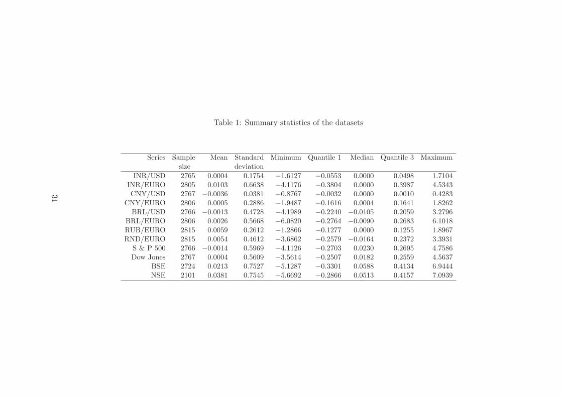
Table 1: Summary statistics of the datasets

Series Sample Mean Standard Minimum Quantile 1 Median Quantile 3 Maximumsize deviation

INR/USD 2765 0.0004 0.1754 −1.6127 −0.0553 0.0000 0.0498 1.7104INR/EURO 2805 0.0103 0.6638 −4.1176 −0.3804 0.0000 0.3987 4.5343CNY/USD 2767 −0.0036 0.0381 −0.8767 −0.0032 0.0000 0.0010 0.4283

CNY/EURO 2806 0.0005 0.2886 −1.9487 −0.1616 0.0004 0.1641 1.8262BRL/USD 2766 −0.0013 0.4728 −4.1989 −0.2240 −0.0105 0.2059 3.2796

BRL/EURO 2806 0.0026 0.5668 −6.0820 −0.2764 −0.0090 0.2683 6.1018RUB/EURO 2815 0.0059 0.2612 −1.2866 −0.1277 0.0000 0.1255 1.8967RND/EURO 2815 0.0054 0.4612 −3.6862 −0.2579 −0.0164 0.2372 3.3931

S & P 500 2766 −0.0014 0.5969 −4.1126 −0.2703 0.0230 0.2695 4.7586Dow Jones 2767 0.0004 0.5609 −3.5614 −0.2507 0.0182 0.2559 4.5637

BSE 2724 0.0213 0.7527 −5.1287 −0.3301 0.0588 0.4134 6.9444NSE 2101 0.0381 0.7545 −5.6692 −0.2866 0.0513 0.4157 7.0939

31

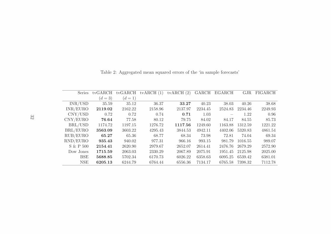
Table 2: Aggregated mean squared errors of the ‘in sample forecasts’

Series tvGARCH tvGARCH tvARCH (1) tvARCH (2) GARCH EGARCH GJR FIGARCH(d = 3) (d = 1)

INR/USD 35.59 35.12 36.37 33.27 40.23 38.03 40.26 38.68INR/EURO 2119.02 2162.22 2158.96 2137.97 2234.45 2524.83 2234.46 2249.93CNY/USD 0.72 0.72 0.74 0.71 1.03 − 1.22 0.96

CNY/EURO 76.64 77.58 80.12 79.75 84.02 84.17 84.55 85.73BRL/USD 1174.72 1197.15 1276.72 1117.56 1249.60 1163.88 1312.59 1221.22

BRL/EURO 3563.09 3603.22 4295.43 3844.53 4942.11 4402.06 5320.83 4861.54RUB/EURO 65.27 65.36 68.77 68.34 73.98 72.81 74.04 69.34RND/EURO 935.43 940.02 977.31 966.16 993.15 981.79 1016.55 989.07

S & P 500 2154.41 2620.90 2979.67 2652.07 2614.41 2476.76 2679.29 2572.90Dow Jones 1715.59 2063.03 2330.29 2067.89 2075.91 1951.45 2125.98 2025.00

BSE 5688.85 5702.34 6170.73 6026.22 6358.63 6095.25 6539.42 6381.01NSE 6205.13 6244.79 6764.44 6556.36 7134.17 6765.58 7398.32 7112.78

32

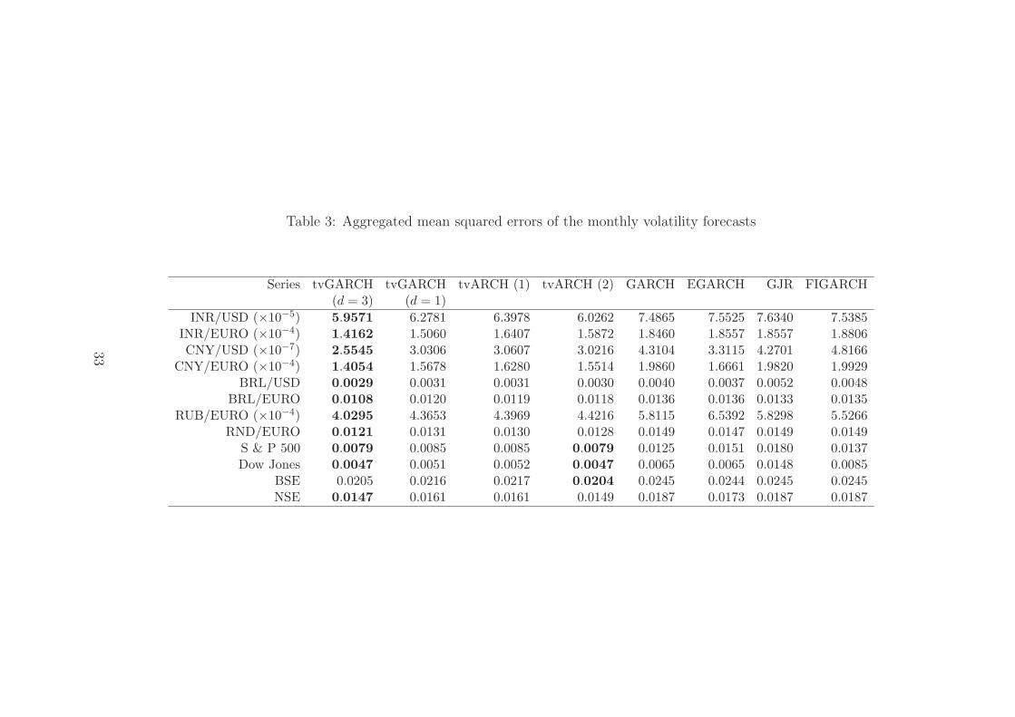
Table 3: Aggregated mean squared errors of the monthly volatility forecasts

Series tvGARCH tvGARCH tvARCH (1) tvARCH (2) GARCH EGARCH GJR FIGARCH(d = 3) (d = 1)

INR/USD (×10−5) 5.9571 6.2781 6.3978 6.0262 7.4865 7.5525 7.6340 7.5385INR/EURO (×10−4) 1.4162 1.5060 1.6407 1.5872 1.8460 1.8557 1.8557 1.8806CNY/USD (×10−7) 2.5545 3.0306 3.0607 3.0216 4.3104 3.3115 4.2701 4.8166

CNY/EURO (×10−4) 1.4054 1.5678 1.6280 1.5514 1.9860 1.6661 1.9820 1.9929BRL/USD 0.0029 0.0031 0.0031 0.0030 0.0040 0.0037 0.0052 0.0048

BRL/EURO 0.0108 0.0120 0.0119 0.0118 0.0136 0.0136 0.0133 0.0135RUB/EURO (×10−4) 4.0295 4.3653 4.3969 4.4216 5.8115 6.5392 5.8298 5.5266

RND/EURO 0.0121 0.0131 0.0130 0.0128 0.0149 0.0147 0.0149 0.0149S & P 500 0.0079 0.0085 0.0085 0.0079 0.0125 0.0151 0.0180 0.0137Dow Jones 0.0047 0.0051 0.0052 0.0047 0.0065 0.0065 0.0148 0.0085

BSE 0.0205 0.0216 0.0217 0.0204 0.0245 0.0244 0.0245 0.0245NSE 0.0147 0.0161 0.0161 0.0149 0.0187 0.0173 0.0187 0.0187

33

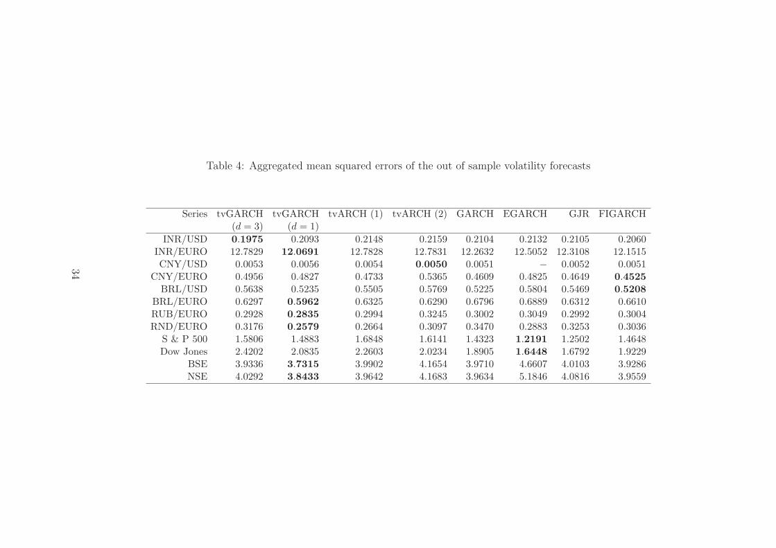
Table 4: Aggregated mean squared errors of the out of sample volatility forecasts

Series tvGARCH tvGARCH tvARCH (1) tvARCH (2) GARCH EGARCH GJR FIGARCH(d = 3) (d = 1)

INR/USD 0.1975 0.2093 0.2148 0.2159 0.2104 0.2132 0.2105 0.2060INR/EURO 12.7829 12.0691 12.7828 12.7831 12.2632 12.5052 12.3108 12.1515CNY/USD 0.0053 0.0056 0.0054 0.0050 0.0051 − 0.0052 0.0051

CNY/EURO 0.4956 0.4827 0.4733 0.5365 0.4609 0.4825 0.4649 0.4525

BRL/USD 0.5638 0.5235 0.5505 0.5769 0.5225 0.5804 0.5469 0.5208

BRL/EURO 0.6297 0.5962 0.6325 0.6290 0.6796 0.6889 0.6312 0.6610RUB/EURO 0.2928 0.2835 0.2994 0.3245 0.3002 0.3049 0.2992 0.3004RND/EURO 0.3176 0.2579 0.2664 0.3097 0.3470 0.2883 0.3253 0.3036

S & P 500 1.5806 1.4883 1.6848 1.6141 1.4323 1.2191 1.2502 1.4648Dow Jones 2.4202 2.0835 2.2603 2.0234 1.8905 1.6448 1.6792 1.9229

BSE 3.9336 3.7315 3.9902 4.1654 3.9710 4.6607 4.0103 3.9286NSE 4.0292 3.8433 3.9642 4.1683 3.9634 5.1846 4.0816 3.9559

34

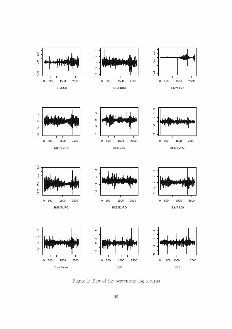
INR/USD

0 500 1500 2500

−1

.50

.01

.0

INR/EURO

0 500 1500 2500

−4

−2

02

4

CNY/USD

0 500 1500 2500

−0

.8−

0.2

0.2

CNY/EURO

0 500 1500 2500

−2

−1

01

BRL/USD

0 500 1500 2500

−4

−2

02

BRL/EURO

0 500 1500 2500

−6

−2

24

6

RUB/EURO

0 500 1500 2500

−1

.00

.01

.02

.0

RND/EURO

0 500 1500 2500

−3

−1

13

S & P 500

0 500 1500 2500

−4

−2

02

4

Dow Jones

0 500 1500 2500

−2

02

4

BSE

0 500 1500 2500

−4

02

46

NSE

0 500 1000 2000

−6

−2

24

6

Figure 1: Plot of the percentage log returns

35

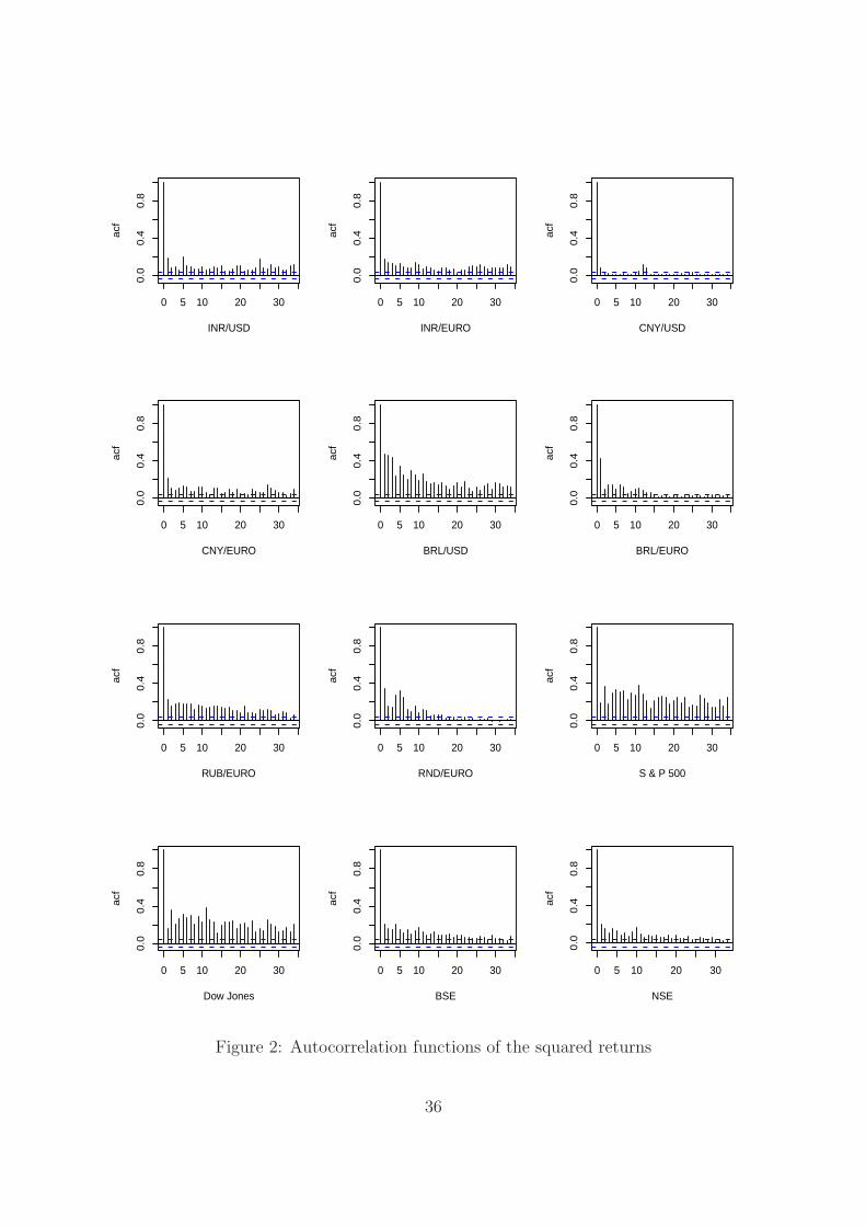
0 5 10 20 30

0.0

0.4

0.8

INR/USD

acf

0 5 10 20 30

0.0

0.4

0.8

INR/EUROa

cf

0 5 10 20 30

0.0

0.4

0.8

CNY/USD

acf

0 5 10 20 30

0.0

0.4

0.8

CNY/EURO

acf

0 5 10 20 30

0.0

0.4

0.8

BRL/USD

acf

0 5 10 20 30

0.0

0.4

0.8

BRL/EUROa

cf

0 5 10 20 30

0.0

0.4

0.8

RUB/EURO

acf

0 5 10 20 30

0.0

0.4

0.8

RND/EURO

acf

0 5 10 20 30

0.0

0.4

0.8

S & P 500

acf

0 5 10 20 30

0.0

0.4

0.8

Dow Jones

acf

0 5 10 20 30

0.0

0.4

0.8

BSE

acf

0 5 10 20 30

0.0

0.4

0.8

NSE

acf

Figure 2: Autocorrelation functions of the squared returns

36

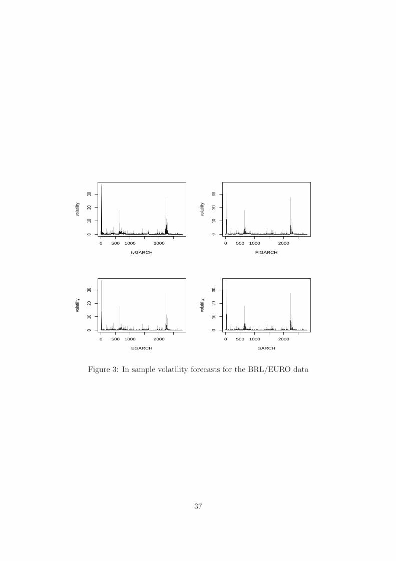
tvGARCH

vola

tility

0 500 1000 2000

010

2030

FIGARCH

vola

tility

0 500 1000 2000

010

2030

EGARCH

vola

tility

0 500 1000 2000

010

2030

GARCH

vola

tility

0 500 1000 2000

010

2030

Figure 3: In sample volatility forecasts for the BRL/EURO data

37

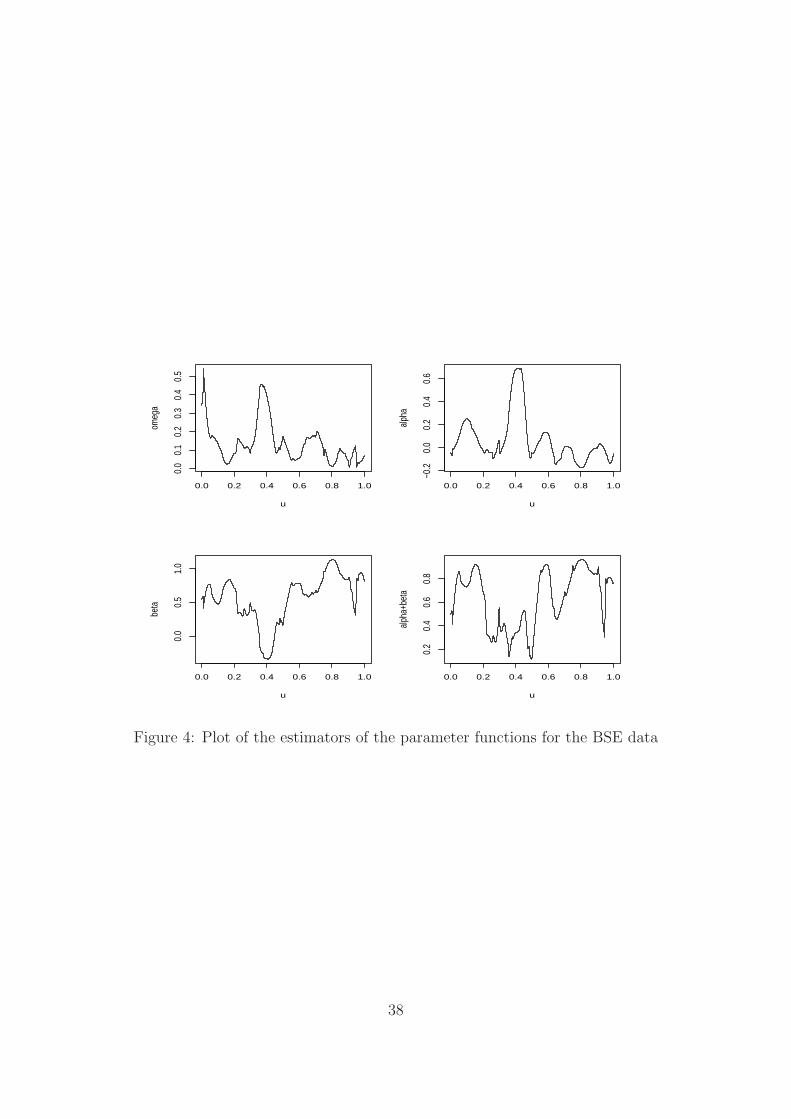
0.0 0.2 0.4 0.6 0.8 1.0

0.0

0.1

0.2

0.3

0.4

0.5

u

omeg

a

0.0 0.2 0.4 0.6 0.8 1.0

−0.2

0.0

0.2

0.4

0.6

u

alph

a

0.0 0.2 0.4 0.6 0.8 1.0

0.0

0.5

1.0

u

beta

0.0 0.2 0.4 0.6 0.8 1.0

0.2

0.4

0.6

0.8

u

alph

a+be

ta

Figure 4: Plot of the estimators of the parameter functions for the BSE data

38