Rotating parametric instability in early Earth
11
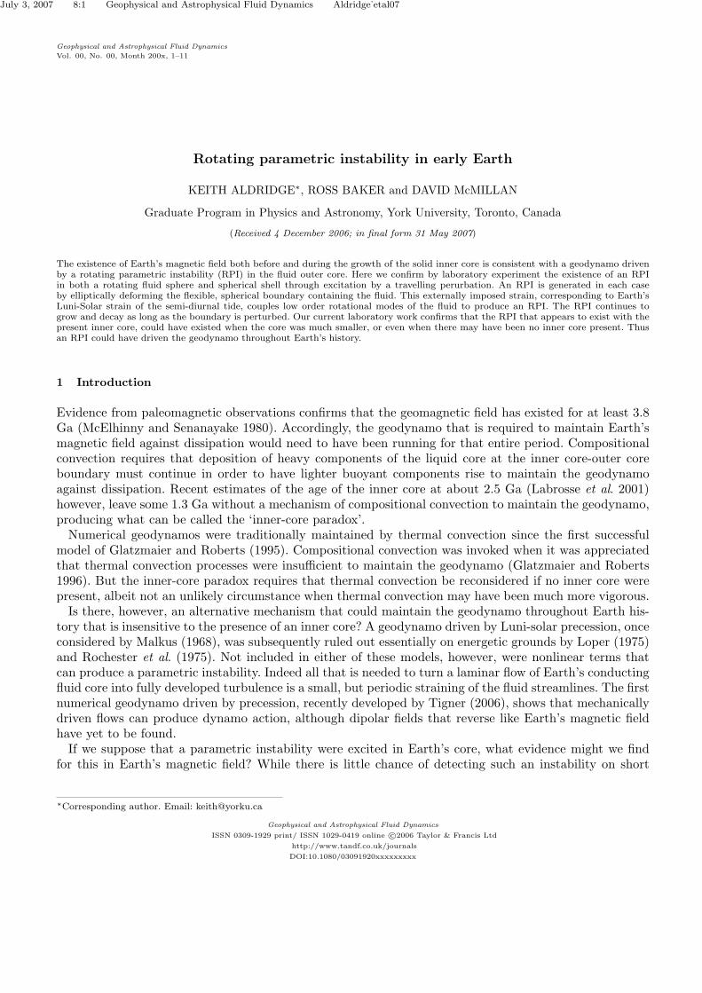
July 3, 2007 8:1 Geophysical and Astrophysical Fluid Dynamics Aldridge˙etal07 Geophysical and Astrophysical Fluid Dynamics Vol. 00, No. 00, Month 200x, 1–11 Rotating parametric instability in early Earth KEITH ALDRIDGE * , ROSS BAKER and DAVID McMILLAN Graduate Program in Physics and Astronomy, York University, Toronto, Canada (Received 4 December 2006; in final form 31 May 2007) The existence of Earth’s magnetic field both before and during the growth of the solid inner core is consistent with a geodynamo driven by a rotating parametric instability (RPI) in the fluid outer core. Here we confirm by laboratory experiment the existence of an RPI in both a rotating fluid sphere and spherical shell through excitation by a travelling perurbation. An RPI is generated in each case by elliptically deforming the flexible, spherical boundary containing the fluid. This externally imposed strain, corresponding to Earth’s Luni-Solar strain of the semi-diurnal tide, couples low order rotational modes of the fluid to produce an RPI. The RPI continues to grow and decay as long as the boundary is perturbed. Our current laboratory work confirms that the RPI that appears to exist with the present inner core, could have existed when the core was much smaller, or even when there may have been no inner core present. Thus an RPI could have driven the geodynamo throughout Earth’s history. 1 Introduction Evidence from paleomagnetic observations confirms that the geomagnetic field has existed for at least 3.8 Ga (McElhinny and Senanayake 1980). Accordingly, the geodynamo that is required to maintain Earth’s magnetic field against dissipation would need to have been running for that entire period. Compositional convection requires that deposition of heavy components of the liquid core at the inner core-outer core boundary must continue in order to have lighter buoyant components rise to maintain the geodynamo against dissipation. Recent estimates of the age of the inner core at about 2.5 Ga (Labrosse et al. 2001) however, leave some 1.3 Ga without a mechanism of compositional convection to maintain the geodynamo, producing what can be called the ‘inner-core paradox’. Numerical geodynamos were traditionally maintained by thermal convection since the first successful model of Glatzmaier and Roberts (1995). Compositional convection was invoked when it was appreciated that thermal convection processes were insufficient to maintain the geodynamo (Glatzmaier and Roberts 1996). But the inner-core paradox requires that thermal convection be reconsidered if no inner core were present, albeit not an unlikely circumstance when thermal convection may have been much more vigorous. Is there, however, an alternative mechanism that could maintain the geodynamo throughout Earth his- tory that is insensitive to the presence of an inner core? A geodynamo driven by Luni-solar precession, once considered by Malkus (1968), was subsequently ruled out essentially on energetic grounds by Loper (1975) and Rochester et al. (1975). Not included in either of these models, however, were nonlinear terms that can produce a parametric instability. Indeed all that is needed to turn a laminar flow of Earth’s conducting fluid core into fully developed turbulence is a small, but periodic straining of the fluid streamlines. The first numerical geodynamo driven by precession, recently developed by Tigner (2006), shows that mechanically driven flows can produce dynamo action, although dipolar fields that reverse like Earth’s magnetic field have yet to be found. If we suppose that a parametric instability were excited in Earth’s core, what evidence might we find for this in Earth’s magnetic field? While there is little chance of detecting such an instability on short * Corresponding author. Email: [email protected] Geophysical and Astrophysical Fluid Dynamics ISSN 0309-1929 print/ ISSN 1029-0419 online c 2006 Taylor & Francis Ltd http://www.tandf.co.uk/journals DOI:10.1080/03091920xxxxxxxxx
Transcript of Rotating parametric instability in early Earth
July 3, 2007 8:1 Geophysical and Astrophysical Fluid Dynamics Aldridge˙etal07
Geophysical and Astrophysical Fluid Dynamics
Vol. 00, No. 00, Month 200x, 1–11
Rotating parametric instability in early Earth
KEITH ALDRIDGE∗, ROSS BAKER and DAVID McMILLAN
Graduate Program in Physics and Astronomy, York University, Toronto, Canada
(Received 4 December 2006; in final form 31 May 2007)
The existence of Earth’s magnetic field both before and during the growth of the solid inner core is consistent with a geodynamo drivenby a rotating parametric instability (RPI) in the fluid outer core. Here we confirm by laboratory experiment the existence of an RPIin both a rotating fluid sphere and spherical shell through excitation by a travelling perurbation. An RPI is generated in each caseby elliptically deforming the flexible, spherical boundary containing the fluid. This externally imposed strain, corresponding to Earth’sLuni-Solar strain of the semi-diurnal tide, couples low order rotational modes of the fluid to produce an RPI. The RPI continues togrow and decay as long as the boundary is perturbed. Our current laboratory work confirms that the RPI that appears to exist with thepresent inner core, could have existed when the core was much smaller, or even when there may have been no inner core present. Thusan RPI could have driven the geodynamo throughout Earth’s history.
1 Introduction
Evidence from paleomagnetic observations confirms that the geomagnetic field has existed for at least 3.8Ga (McElhinny and Senanayake 1980). Accordingly, the geodynamo that is required to maintain Earth’smagnetic field against dissipation would need to have been running for that entire period. Compositionalconvection requires that deposition of heavy components of the liquid core at the inner core-outer coreboundary must continue in order to have lighter buoyant components rise to maintain the geodynamoagainst dissipation. Recent estimates of the age of the inner core at about 2.5 Ga (Labrosse et al. 2001)however, leave some 1.3 Ga without a mechanism of compositional convection to maintain the geodynamo,producing what can be called the ‘inner-core paradox’.
Numerical geodynamos were traditionally maintained by thermal convection since the first successfulmodel of Glatzmaier and Roberts (1995). Compositional convection was invoked when it was appreciatedthat thermal convection processes were insufficient to maintain the geodynamo (Glatzmaier and Roberts1996). But the inner-core paradox requires that thermal convection be reconsidered if no inner core werepresent, albeit not an unlikely circumstance when thermal convection may have been much more vigorous.
Is there, however, an alternative mechanism that could maintain the geodynamo throughout Earth his-tory that is insensitive to the presence of an inner core? A geodynamo driven by Luni-solar precession, onceconsidered by Malkus (1968), was subsequently ruled out essentially on energetic grounds by Loper (1975)and Rochester et al. (1975). Not included in either of these models, however, were nonlinear terms thatcan produce a parametric instability. Indeed all that is needed to turn a laminar flow of Earth’s conductingfluid core into fully developed turbulence is a small, but periodic straining of the fluid streamlines. The firstnumerical geodynamo driven by precession, recently developed by Tigner (2006), shows that mechanicallydriven flows can produce dynamo action, although dipolar fields that reverse like Earth’s magnetic fieldhave yet to be found.
If we suppose that a parametric instability were excited in Earth’s core, what evidence might we findfor this in Earth’s magnetic field? While there is little chance of detecting such an instability on short
∗Corresponding author. Email: [email protected]
Geophysical and Astrophysical Fluid Dynamics
ISSN 0309-1929 print/ ISSN 1029-0419 online c©2006 Taylor & Francis Ltd
http://www.tandf.co.uk/journals
DOI:10.1080/03091920xxxxxxxxx
July 3, 2007 8:1 Geophysical and Astrophysical Fluid Dynamics Aldridge˙etal07
2 Rotating parametric instability in early Earth
timescales, the growth and decay of an instability should be preserved in the paleomagnetic record. Aldridgeand Baker (2003) searched records of relative paleointensity from a site in the North Atlantic with a highsedimentation rate and took the temporal behaviour of the magnetic intensity as a proxy for the fluidvelocity (Moffatt 1978). Thus the growth and decay of the field was interpreted as a measure of thecorresponding growth and decay of a parametric instability in Earth’s core. Subsequently these authorsanalyzed several sets of both single records and composite stacks of relative paleointensity, finding that thetimescales of growth and decay were consistent with what would be expected from straining of streamlinesof the fluid core by the gradient of the Luni-solar gravitational field.
Earth responds to the Luni-solar gradient in two primary ways. First, due to its slightly oblate figure,Earth’s rotation axis precesses with an amplitude of 23.5 degrees at a period of approximately 25800yr. This precession produces a predominant shearing of fluid streamlines in Earth’s core, which will leadto a parametric instability if dissipation in the core is sufficiently small. Second, ellipsoidal distortion ofequipotentials is evident on Earth as the solid Earth tide. Straining of otherwise circular streamlines inEarth’s core into ellipses also produces a travelling parametric instability since the Lunar and Solar daysare longer than the sidereal day. The laboratory experiments described in this paper are the counterpartsof this travelling elliptical instability.
Strains, ε, that couple rotational core modes are proportional to the gradient of Luni-solar gravitationalfield. These small strains, corresponding to millennial geomagnetic time scales, have existed throughoutEarth history. A kinematic geodynamo has been shown possible if the flow has specific dynamical proper-ties. Rotational modes, for example, which are coupled by elliptical strain, have their vorticity coincidingwith their velocity and can produce an α-dynamo (Olson 1981). A dynamo driven by a travelling ellipticalinstability avoids the inner-core paradox as long as the instability can be excited both with and withoutan inner core.
Properties of parametric instability of a rotating fluid, or rotating parametric instability (RPI), weregiven recently in theoretical work by Kerswell (1993). Inertial or rotational modes of a contained, idealfluid sphere have frequencies λnmk=ωnmk/Ω, where (0 < λnmk < 2) and Ω is the fluid’s rotation speed.The indices (n,m) give the modal structure in the plane containing the rotation axis of the fluid, whilek = 0,±1,±2, ... is the azimuthal wavenumber of the mode. Elliptical deformation of the fluid’s streamlineswill couple two inertial modes with wavenumbers k1 − k2 = 2 and frequencies λnmk1 − λnmk2 = 2, whileshearing of streamlines will couple two inertial modes with wavenumbers k1 − k2 = 1 and frequenciesλnmk1 − λnmk2 = 1.
Work on parametric instabilities in a cylindrical geometry dates back to Gledzer et al. (1975) who studiedelliptical instability in rotating elliptically deformed cylindrical cavities, and later by Vladimirov andTarasov (1985). Later Malkus (1989) and more recently Eloy et al. (2000) excited the elliptical instability ina rotating cylindrical cavity by deforming its external boundary through sets of rollers that were stationaryin the laboratory frame of reference. Work on parametic instability in an ellipsoidal cavity was pioneered byBoubnov (1978). Subsequently elliptical instability was excited in a full sphere by Lacaze et al. (2004) usinga stationary external perturbation and in 35% shells by Aldridge et al. (1997) and Seyed-Mahmoud et al.(2004) using a travelling internal perturbation. Lacaze et al. (2005) have excited parametric instabilitywith a stationary, external perturbation in a 30% shell and found excellent agreement with a model basedon linear stability theory. In summary, the existence of parametric instability has been confirmed underthe following circumstances: excited by a stationary perturbation in a full sphere and a 30% shell (Lacazeet al. 2004, 2005); and excited by a travelling perturbation in a 35% shell (Seyed-Mahmoud et al. 2004).The present work uses a travelling perturbation to confirm the existence of a parametric instability in a22% shell and a full sphere, which correspond to the geophysical case of an early Earth. The previousresult for travelling perturbation in a 35% shell corresponds to the present Earth.
2 Experimental Configuration
Excitation and measurement of an RPI in both a sphere and a spherical shell through a travelling pertur-bation determined the design of our experiment. Here, elliptical straining of the streamlines is producedby a retrograde-rotating set of rollers that deform the outer boundary, while the container itself rotates in
July 3, 2007 8:1 Geophysical and Astrophysical Fluid Dynamics Aldridge˙etal07
Rotating parametric instability in early Earth 3
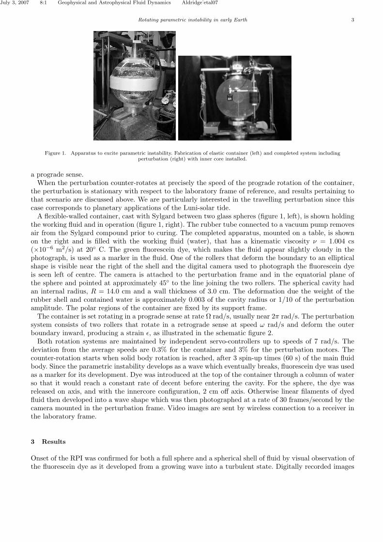
Figure 1. Apparatus to excite parametric instability. Fabrication of elastic container (left) and completed system includingperturbation (right) with inner core installed.
a prograde sense.When the perturbation counter-rotates at precisely the speed of the prograde rotation of the container,
the perturbation is stationary with respect to the laboratory frame of reference, and results pertaining tothat scenario are discussed above. We are particularly interested in the travelling perturbation since thiscase corresponds to planetary applications of the Luni-solar tide.
A flexible-walled container, cast with Sylgard between two glass spheres (figure 1, left), is shown holdingthe working fluid and in operation (figure 1, right). The rubber tube connected to a vacuum pump removesair from the Sylgard compound prior to curing. The completed apparatus, mounted on a table, is shownon the right and is filled with the working fluid (water), that has a kinematic viscosity ν = 1.004 cs(×10−6 m2/s) at 20 C. The green fluorescein dye, which makes the fluid appear slightly cloudy in thephotograph, is used as a marker in the fluid. One of the rollers that deform the boundary to an ellipticalshape is visible near the right of the shell and the digital camera used to photograph the fluorescein dyeis seen left of centre. The camera is attached to the perturbation frame and in the equatorial plane ofthe sphere and pointed at approximately 45 to the line joining the two rollers. The spherical cavity hadan internal radius, R = 14.0 cm and a wall thickness of 3.0 cm. The deformation due the weight of therubber shell and contained water is approximately 0.003 of the cavity radius or 1/10 of the perturbationamplitude. The polar regions of the container are fixed by its support frame.
The container is set rotating in a prograde sense at rate Ω rad/s, usually near 2π rad/s. The perturbationsystem consists of two rollers that rotate in a retrograde sense at speed ω rad/s and deform the outerboundary inward, producing a strain ε, as illustrated in the schematic figure 2.
Both rotation systems are maintained by independent servo-controllers up to speeds of 7 rad/s. Thedeviation from the average speeds are 0.3% for the container and 3% for the perturbation motors. Thecounter-rotation starts when solid body rotation is reached, after 3 spin-up times (60 s) of the main fluidbody. Since the parametric instability develops as a wave which eventually breaks, fluorescein dye was usedas a marker for its development. Dye was introduced at the top of the container through a column of waterso that it would reach a constant rate of decent before entering the cavity. For the sphere, the dye wasreleased on axis, and with the innercore configuration, 2 cm off axis. Otherwise linear filaments of dyedfluid then developed into a wave shape which was then photographed at a rate of 30 frames/second by thecamera mounted in the perturbation frame. Video images are sent by wireless connection to a receiver inthe laboratory frame.
3 Results
Onset of the RPI was confirmed for both a full sphere and a spherical shell of fluid by visual observation ofthe fluorescein dye as it developed from a growing wave into a turbulent state. Digitally recorded images
July 3, 2007 8:1 Geophysical and Astrophysical Fluid Dynamics Aldridge˙etal07
4 Rotating parametric instability in early Earth
Ω
ω
camera
Roller
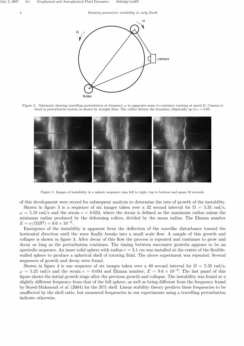
Figure 2. Schematic showing travelling perturbation at frequency ω in oppposite sense to container rotating at speed Ω. Camera isfixed in perturbation system as shown by straight lines. The rollers deform the boundary elliptically up to ε = 0.05.
Figure 3. Images of instability in a sphere; sequence runs left to right, top to bottom and spans 32 seconds.
of this development were stored for subsequent analysis to determine the rate of growth of the instability.Shown in figure 3 is a sequence of six images taken over a 32 second interval for Ω = 5.35 rad/s,
ω = 5.18 rad/s and the strain ε = 0.034, where the strain is defined as the maximum radius minus theminimum radius produced by the deforming rollers, divided by the mean radius. The Ekman numberE = ν/(ΩR2) = 9.6× 10⁻⁶.
Emergence of the instability is apparent from the deflection of the wavelike disturbance toward thehorizontal direction until the wave finally breaks into a small scale flow. A sample of this growth andcollapse is shown in figure 3. After decay of this flow the process is repeated and continues to grow anddecay as long as the perturbation continues. The timing between successive growths appears to be anaperiodic sequence. An inner solid sphere with radius r = 3.1 cm was installed at the centre of the flexible-walled sphere to produce a spherical shell of rotating fluid. The above experiment was repeated. Severalsequences of growth and decay were found.
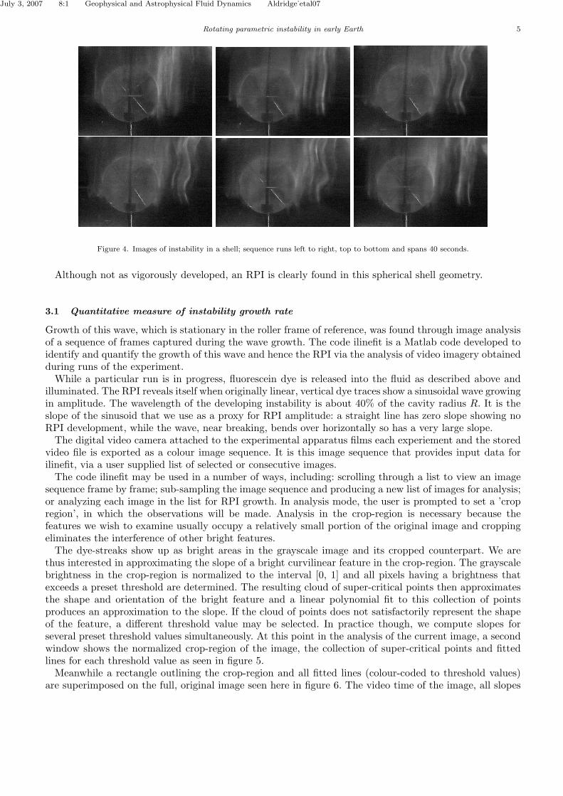
Shown in figure 4 is one sequence of six images taken over a 40 second interval for Ω = 5.35 rad/s,ω = 5.25 rad/s and the strain ε = 0.034 and Ekman number, E = 9.6 × 10⁻⁶. The last panel of thisfigure shows the initial growth stage after the previous growth and collapse. The instability was found at aslightly different frequency from that of the full sphere, as well as being different from the frequency foundby Seyed-Mahmoud et al. (2004) for the 35% shell. Linear stability theory predicts these frequencies to beunaffected by the shell ratio, but measured frequencies in our experiments using a travelling perturbationindicate otherwise.
July 3, 2007 8:1 Geophysical and Astrophysical Fluid Dynamics Aldridge˙etal07
Rotating parametric instability in early Earth 5
Figure 4. Images of instability in a shell; sequence runs left to right, top to bottom and spans 40 seconds.
Although not as vigorously developed, an RPI is clearly found in this spherical shell geometry.
3.1 Quantitative measure of instability growth rate
Growth of this wave, which is stationary in the roller frame of reference, was found through image analysisof a sequence of frames captured during the wave growth. The code ilinefit is a Matlab code developed toidentify and quantify the growth of this wave and hence the RPI via the analysis of video imagery obtainedduring runs of the experiment.
While a particular run is in progress, fluorescein dye is released into the fluid as described above andilluminated. The RPI reveals itself when originally linear, vertical dye traces show a sinusoidal wave growingin amplitude. The wavelength of the developing instability is about 40% of the cavity radius R. It is theslope of the sinusoid that we use as a proxy for RPI amplitude: a straight line has zero slope showing noRPI development, while the wave, near breaking, bends over horizontally so has a very large slope.
The digital video camera attached to the experimental apparatus films each experiement and the storedvideo file is exported as a colour image sequence. It is this image sequence that provides input data forilinefit, via a user supplied list of selected or consecutive images.
The code ilinefit may be used in a number of ways, including: scrolling through a list to view an imagesequence frame by frame; sub-sampling the image sequence and producing a new list of images for analysis;or analyzing each image in the list for RPI growth. In analysis mode, the user is prompted to set a ’cropregion’, in which the observations will be made. Analysis in the crop-region is necessary because thefeatures we wish to examine usually occupy a relatively small portion of the original image and croppingeliminates the interference of other bright features.
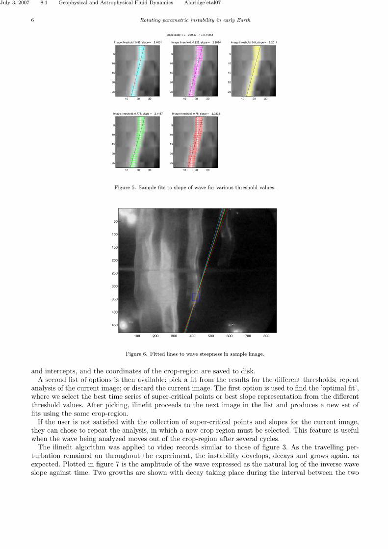
The dye-streaks show up as bright areas in the grayscale image and its cropped counterpart. We arethus interested in approximating the slope of a bright curvilinear feature in the crop-region. The grayscalebrightness in the crop-region is normalized to the interval [0, 1] and all pixels having a brightness thatexceeds a preset threshold are determined. The resulting cloud of super-critical points then approximatesthe shape and orientation of the bright feature and a linear polynomial fit to this collection of pointsproduces an approximation to the slope. If the cloud of points does not satisfactorily represent the shapeof the feature, a different threshold value may be selected. In practice though, we compute slopes forseveral preset threshold values simultaneously. At this point in the analysis of the current image, a secondwindow shows the normalized crop-region of the image, the collection of super-critical points and fittedlines for each threshold value as seen in figure 5.
Meanwhile a rectangle outlining the crop-region and all fitted lines (colour-coded to threshold values)are superimposed on the full, original image seen here in figure 6. The video time of the image, all slopes
July 3, 2007 8:1 Geophysical and Astrophysical Fluid Dynamics Aldridge˙etal07
6 Rotating parametric instability in early Earth
Image threshold: 0.85; slope = 2.4001
10 20 30
5
10
15
20
25
Image threshold: 0.825; slope = 2.3024
10 20 30
5
10
15
20
25
Image threshold: 0.8; slope = 2.2011
10 20 30
5
10
15
20
25
Image threshold: 0.775; slope = 2.1467
10 20 30
5
10
15
20
25
Slope stats: ∝ = 2.2147; = 0.14454
Image threshold: 0.75; slope = 2.0232
10 20 30
5
10
15
20
25
σ
Figure 5. Sample fits to slope of wave for various threshold values.
100 200 300 400 500 600 700 800
50
100
150
200
250
300
350
400
450
Figure 6. Fitted lines to wave steepness in sample image.
and intercepts, and the coordinates of the crop-region are saved to disk.A second list of options is then available: pick a fit from the results for the different thresholds; repeat
analysis of the current image; or discard the current image. The first option is used to find the ’optimal fit’,where we select the best time series of super-critical points or best slope representation from the differentthreshold values. After picking, ilinefit proceeds to the next image in the list and produces a new set offits using the same crop-region.
If the user is not satisfied with the collection of super-critical points and slopes for the current image,they can chose to repeat the analysis, in which a new crop-region must be selected. This feature is usefulwhen the wave being analyzed moves out of the crop-region after several cycles.
The ilinefit algorithm was applied to video records similar to those of figure 3. As the travelling per-turbation remained on throughout the experiment, the instability develops, decays and grows again, asexpected. Plotted in figure 7 is the amplitude of the wave expressed as the natural log of the inverse waveslope against time. Two growths are shown with decay taking place during the interval between the two

July 3, 2007 8:1 Geophysical and Astrophysical Fluid Dynamics Aldridge˙etal07
Rotating parametric instability in early Earth 7
20 30 40 50 60 70 80 90 100 110−2
−1.5
−1
−0.5
0
0.5
1 Full Sphere
Time (s)
Am
plitu
de
τ = 18.60 s
τ = 10.50 s
Figure 7. Sample growths of instability after the perturbation remained turned on for several cycles of growth and decay. Onlygrowths are recorded and τ values are measured e-folding times of the instability’s growth.
20 30 40 50 60 70 80 90 100 110 2
1.5
1
0.5
0
0.5
1 Spherical Shell
Time (s)
Am
plit
ude τ = 7.36 s
Figure 8. Growth of instability in 22% shell.
growths.Shown in figure 8 are the measured amplitudes of the growing instability in the 22% shell for the same
experimental parameters as those for figure 4. After several susbsequent growths and decays in the shellgeometry, evidence for what can be termed a two-stage growth was observed as illustrated in figure 9. Thisphenomenon of a double growth was only oberved intermittenly but it’s presence is certain.
4 Oceanic records of relative paleointensity
If the instability found in our laboratory experiments is excited in Earth’s fluid core through straining ofthe core by the gradient of the Luni-solar gravity field, evidence of this fact should be found in Earth’spaleomagnetic field. We assume here that the spectral properties of the observed magnetic field will bea proxy for that of the velocity (Moffatt 1978). Reported by Baker et al. (2006) are six sequences ofpaleomagnetic intensity that those authors have searched for evidence of RPI in Earth’s core. Threesequences (WCB, ODP983, ODP1062) were from single sites while three were from composite stacks(NAPIS-75, GLOPIS-75, SINT2000) comprising several records. All data studied was from the interval 0-80ka. Significant errors in timing as well as amplitude will certainly result and these have been considered inBaker et al. (2006). Also studied in that paper are constraints on the use of stacked records, in comparisonwith single core composites. Details of the sources of this data are given in Baker et al. (2006).

July 3, 2007 8:1 Geophysical and Astrophysical Fluid Dynamics Aldridge˙etal07
8 Rotating parametric instability in early Earth
20 30 40 50 60 70 80 90 100 110 2
1.5
1
0.5
0
0.5
1Spherical Shell, 2 Stage Growth
Time (s)
Am
plit
ude
τ = 20.81 s
τ = 3.91 s
Figure 9. Example of two-stage growth of instability in 22% shell.
4.1 Growth and Decay of Relative Paleointensity
Exponential growths and decays of intensity would be expected if these changes in amplitude were due toan RPI in Earth’s core. Baker et al. (2006) identified several intervals of growth and decay and found bestfitting exponentials for each of the segments they identified. After examining the three composite stacksby computing coherence spectra between pairs of records constituting the stacks, Baker et al. (2006) foundthat no reliable information could be obtained from the SINT2000 stack for time intervals shorter thanabout 20 kyr. Thus smoothing through the stacking of some 34 individual records has removed any possibleevidence of the signature expected for parametric instability.
4.2 Modeling the Data
From linear stability theory (Kerswell 1993) the observed growth rate is (αε−βE1/2)Ω while the observeddecay is βE1/2Ω where ε is the perturbation amplitude, E is the Ekman number and Ω is the fluid’srotation speed. α, β are typically of order unity. While bulk dissipation will certainly occur at rate EΩ,it is the boundary layer dissipation at rate βE1/2Ω, corresponding to the decay of the modes driving thedynamo, that are relevant here. Accordingly, an ideal growth rate, αεΩ can be estimated by summingsequential growths and decays.
4.3 Predictions from Linear Stability Theory (LST)
We can calculate an ideal growth rate expected for Earth’s core for each of two sources of straining in thecore. The semi-diurnal tide is expected to give a predominantly elliptical strain, while precession of mantlewill produce mainly a shearing in the core (Kerswell 1993). Table 1 lists the ideal growth rates expectedfrom these two sources and expresses the reciprocal of these rates or e-folding times in thousands of years.Clearly the very small tidal strains and very slow precessional rates produced by gradients of Luni-solargravity translate into long time scales that are typical of the ones we see in paleomagnetic data. In thenext section, the rates found from analysing relative paleomagnetic intensities will be converted to ideale-folding times for comparison with those predicted from linear stability theory (LST).
4.4 Observations and Predictions from LST
Reported ideal growth rates for each of 5 paleomagetic intensity sequences yielded mean and standarddeviations in kyr are: WCB (2.5 ± 2.5), ODP983 (3.5 ± 1.9), OPD1062 (2.1 ± 1.2), NAPIS (3.4 ± 0.6),GLOPIS (3.8± 0.9) (Baker et al. 2006).

July 3, 2007 8:1 Geophysical and Astrophysical Fluid Dynamics Aldridge˙etal07
Rotating parametric instability in early Earth 9
Table 1. Predictions of ideal growth rates and e-folding times for tidal (elliptical) and shear (precession) strains in Earth.
Type of Deformation Ideal IdealPerturbation Amplitude Growth E-folding
ε Rate TimeαεΩ
elliptical 8.5× 10⁻⁸ 3.1× 10⁻¹² 10sec−1 kyears
shear 4.0× 10⁻⁸ 1.7× 10⁻¹² 18sec−1 kyears
Table 2. Ideal E-folding times observed and predicted for laboratory experiments and Earth’s core.
Laboratory Earth’s Core(ε = 0.034) (ε = 8.5× 10⁻⁸)
LST 22.0 s 10 kyr
From observations 10.3± 1.8 s 3.6± 0.6 kyr
From the growths given above, the mean ideal e-folding time, weighted with inverse variances from theseobservations, is 3.3± 0.44kyr. Estimates of Ekman numbers from the decay portions of the records, usingβ = 2.62 are WCB (5.5 × 10⁻¹⁵), ODP983 (1.0 × 10⁻¹⁵), OPD1062 (3.3 × 10⁻¹⁵), NAPIS (1.1 × 10⁻¹⁵),GLOPIS (0.7 × 10⁻¹⁵) (Baker et al. 2006). which are consistent with other low estimates of core Ekmannumbers. Coresponding estimates of kinematic viscosity for the core using the core radius as the lengthscale give WCB (4.9×10⁻⁶), ODP983 (0.90×10⁻⁶), OPD1062 (2.9×10⁻⁶), NAPIS (0.98×10⁻⁶), GLOPIS(0.64 × 10⁻⁶) m2 s−1, similar to those of liquid metals. Given the very large range of estimates for coreviscosity (Lumb and Aldridge 1991), this is not a profound result. It is, however, not inconsistent with thepresence of an RPI in Earth’s core produced by gradients in Luni-Solar gravity.
4.5 Evidence for Elliptical Instability in Earth’s core
Laboratory experiments reported here for elliptical strains ε = 0.034 should have produced an ideal e-folding time of about 22 s while observation gave 10.3 s as shown in column 1 of table 2. We use α = 0.5and β = 2.62 for the predicted ideal e-folding times in the experiment based on the observations fromfigure 7 The estimate of the ideal e-folding time from these same observations, found by combining adjacentgrowths and decays, is significantly shorter than predicted by LST. A similar speed-up of Earth responsecompared to LST is found from our observations, which for example yield 3.3 kyr from the paleointensitydata compared to 10 kyr for LST.
Parametric instability has been excited in a fluid sphere contained by a flexible outer wall and in aspherical shell using a travelling perturbation. These experiments confirm the existence of this instabilityin the sphere and spherical shell geometry (Lacaze et al. 2004, 2005) already observed for a stationaryperturbation. While the experiments reported here are consistent with expectation from linear stabilitytheory, the existence of a second growth stage reported here for the 22% shell is indicative of a finiteamplitude stage of growth.
A 22% shell corresponds to an inner core of age approximately 1.6Ga. Both unstable flows were initiatedby externally straining the flexible outer boundary containing the fluid. In earlier experiments RPI wasexcited in a spherical shell by elliptically straining the shell’s inner boundary (Seyed-Mahmoud et al.
July 3, 2007 8:1 Geophysical and Astrophysical Fluid Dynamics Aldridge˙etal07
10 Rotating parametric instability in early Earth
2004). Thus RPI in a fluid shell has been observed through excitation of both inner and outer boundaries.Forced straining throughout the shell as in Earth via tidal straining, however, can only be approximatedin our laboratory experiments through boundary deformations. It is also noteworthy that, unlike in ourexperiments, tidal deformation of the lower mantle would not play a role in the straining of core fluid.Finally, a caution must be made concerning the nature of inertial modes at very low Ekman numbersexpected in Earth’s fluid core. Indeed, the Poincare problem that describes the fluid pressure is hyperbolicin space but has specified boundary conditions, making it ill-posed in the Hadamard sense so that analyticalsolutions are not guaranteed. While there is no problem finding such solutions for a full sphere (Greenspan1969), such is not the case for a spherical shell (Rieutord et al. 2001). At low Ekman numbers complexbehaviour results in spherical shells with the appearance of limit cycles and an increasingly important roleof characteristic surfaces in the fluid.
With the proviso that the above cautions allow, we conclude that a geodynamo driven by RPI would beindependent of the presence of an inner core (Labrosse et al. 2001). This conclusion has been drawn fromthe laboratory experiments reported here using a travelling perurbation and from other recent experimentsthat have shown the existence of parametric instability in both a sphere and spherical shell geometriesexcited by a stationary perturbation (Lacaze et al. 2004, 2005). Analysis of records of relative paleoin-tensity from oceanic cores over the past 80 kyr lend support to the possibility of a geodynamo drivenby parametric instability. Implicit in our conclusion is that the signatures found to be consistent with anelliptical instability in Earth’s core would also exist at earlier epochs of the Luni-Solar gravity field. Whensufficient paleointensity data from those epochs are available it will become possible to use that data tobuild a consistent model for Earth and Moon orbital elements with core properties that determine growthand decay of a rotating parametric instability.
AcknowlegementsWe are grateful to Jerome Noir and an anonymous referee for several important comments which we
believe helped us greatly improve our manuscript. Funding for this work came from a Discovery grantawarded to KDA by the Natural Sciences and Engineering Research Council of Canada.
July 3, 2007 8:1 Geophysical and Astrophysical Fluid Dynamics Aldridge˙etal07
REFERENCES 11
REFERENCES
Aldridge, K. and Baker, R. Paleomagnetic intensity data: A window on the dynamics of Earth’s fluid core?Phys. Earth Planet. Int., 2003. 140, 91–100.
Aldridge, K. D., Seyed-Mahmoud, B., Henderson, G. and van Wijngaarden, W. Elliptical instability ofthe Earth’s fluid core. Phys. Earth Planet. Int., 1997. 103, 365–374.
Baker, R., McMillan, D.and Lumb, I. and Aldridge, K. Chronology errors and their effects on the recoveryof characteristic time scales of the geodynamo from relative paleointensity. Phys. Earth Planet. Int.,2006. 159, 267–275.
Boubnov, B. M. Effect of coriolis force field on the motion of a fluid inside an ellipsoidal cavity. Izv.Atmos. Ocean. Phys., 1978. 14, 501–504.
Eloy, C., Le Gal, P. and Le Dizes, S. Experimental study of the multipolar vortex instability. Phys. Rev.Lett., 2000. 85, 3400–3403.
Glatzmaier, G. A. and Roberts, P. H. A three-dimensional self-consistent computer simulation of a geo-magnetic field reversal. Nature, 1995. 377.
Glatzmaier, G. A. and Roberts, P. H. An anelastic evolutionary geodynamo simulation driven by compo-sitional and thermal convection. j-PhysD , 1996. 97, 81–94.
Gledzer, E., Dolzhansky, F., Obukhov, A. and Ponomarev, V. An experimental and theoretical studyof the stability of motion of a liquid in an elliptical cylinder. Izv. Atmos. Ocean. Phys., 1975. 11,617–622.
Greenspan, H. P. Theory of Rotating Fluids (Cambridge University Press, Cambridge), 1969.Kerswell, R. The instability of precessing flow. Geophys. Astrophys. Fluid Dyn., 1993. 72, 107–114.Labrosse, S., Poirier, J.-P. and J-L, L. M. The age of the inner core. Earth Planet. Sci. Lett., 2001. 190,
11–123.Lacaze, L., Le Gal, P. and Dizes, L. Elliptical instability in a rotating spheroid. J. Fluid Mech., 2004.
505, 1–2.Lacaze, L., Le Gal, P. and Dizes, L. Elliptical instability of a flow in a rotating shell. Phys. Earth Planet.
Int., 2005. 151, 194–205.Loper, D. Torque balance and energy budget for the precessionally driven dynamo. Phys. Earth Planet.
Int., 1975. 11, 43–60.Lumb, L. and Aldridge, K. On viscosity estimates for the Earth’s fluid core. J. Geomagn. Geoelectr., 1991.
43, 93–110.Malkus, W. Precession of the Earth as the cause of geomagnetism. Science, 1968. 160, 259–264.Malkus, W. An experiment study of global instability due to tidal (elliptical) distortion of a rotating
elastic cylinder. Geophys. Astrophys. Fluid Dyn., 1989. 48, 123–134.McElhinny, M. and Senanayake, W. Paleomagnetic evidence of the geomagnetic field 3.5 ga ago. J.
Geophys. Res., 1980. 85, 3523–3528.Moffatt, H. Magnetic field generation in electrically conducting fluids (Cambridge University Press, Cam-
bridge), 1978.Olson, P. A simple physical model for the terrestrial dynamo. j-JGR, 1981. 86, 10875–1088.Rieutord, M., Georgeot, B. and Valdettaro, L. Inertial waves in a rotating spherical shell: attractors and
asymptotic spectrum. J. Fluid Mech., 2001. 435, 103–144.Rochester, M., Jacobs, J., D.E, S. and K.F., C. Can precession power the geomagnetic dynamo? Geophys.
J. Royal Astr. Soc., 1975. 43, 661–678.Seyed-Mahmoud, B., Aldridge, K. D. and Henderson, G. Elliptical instability in rotating ellipsoidal fluid
shells: Application to the Earth’s fluid core,. Phys. Earth Planet. Int., 2004. 142, 257–282.Tigner, A. Precession driven dynamos. Phys. Fluids, B , 2006. 17, 034104.Vladimirov, V. and Tarasov, V. Resonance instability of the flows with closed streamlines. In Laminar-
Turbulent Transition, edited by V. Koslov (Springer, New York), 1985 pp. 717–722, pp. 717–722.