Incompressible flow in porous media with fractional diffusion
Upload
khangminh22Category
view
0download
0
INCOMPRESSIBLE FLUID FLOWS
IN RAPIDLY ROTATING CAVITIES
Alexandre Fournier
A DISSERTATION
PRESENTED TO THE FACULTY
OF PRINCETON UNIVERSITY
IN CANDIDACY FOR THE DEGREE
OF DOCTOR OF PHILOSOPHY
RECOMMENDED FOR ACCEPTANCE
BY THE DEPARTMENT OF
GEOSCIENCES
January 2004
Reminder for Adobe Acrobat ® Reader users: use
• Ctrl + Left Arrow to see previous view,
• Ctrl + Right Arrow to see next view.

© Copyright 2004 by Alexandre Fournier. All rights reserved.

Abstract
The subject of incompressible fluid flows in rapidly rotating cavities, relevant to the dy-namics of the Earth’s outer core, is addressed here by means of numerical modeling. Werecall in the introduction what makes this topic fascinating and challenging, and emphasizethe need for new, more flexible numerical approaches in line with the evolution of today’sparallel computers. Relying upon recent advances in numerical analysis, we first introducein chapter 2 a spectral element model of the axisymmetric Navier-Stokes equation, in a ro-tating reference frame. Comparisons with analytical or published numerical solutions aremade for various test problems, which highlight the spectral convergence properties andadaptivity of the approach. In chapter 3, we couple this axisymmetric kernel with a Fourierexpansion in longitude in order to describe the dynamics of three-dimensional convectiveflows. Again, several reference problems are studied. In the specific case of a rotating fluidundergoing thermal convection, this so-called Fourier-spectral element method (FSEM)proves to be as accurate as standard pseudo-spectral techniques. Having this numericaltool anchored on solid grounds, we study in chapter 4 fluid flows driven by thermal con-vection and precession at the same time. A new topic in the vast field of fluid mechanics,convecto-precessing flows are of particular importance for the Earth’s core, and the equa-tions governing their evolution are derived in detail. We solve these using the FSEM;results seem to indicate that to first order, thermal convection and precession ignore eachother. We discuss the relevance of these calculations for the Earth’s core and outline direc-tions for future related research.
iii

Acknowledgments
The next few paragraphs have been written down quite hastily. This was not a wise thingto do, since they are the only ones that everyone actually reads. Were you not to find yourname, blame it on the inherently erratic behaviour of a Ph.D. candidate in his final hours.
I am grateful to my advisers, Hans-Peter Bunge and Rainer Hollerbach, for their stimulatingremarks and their continuous support over the past five years. Needless to say, I hope thatour fruitful interaction will continue in the future. I thank Tony Dahlen, Guust Nolet, andGeoff Vallis for agreeing to check on my philosophical abilities during my final publicoral examination. I would especially like to thank Tony for the quality of his graduatecourse on Theoretical Geophysics and his –inspiring– quintessential display of scientificattitude. Among the Geosciences faculty, I am grateful to Jason Morgan and Allan Rubinfor showing a continuous interest in my work.
During these five years of graduate school, I have been lucky enough to live with outstand-ing roommates. Let them be praised here (in chronological order): Rupinder ’Nietzsche’Singh, Thierry ’method man’ Huck, Emmanuel and Ariane, Nicolas and Samia, and Raf-faella ’defense coach’ Montelli. In particular, Emmanuel taught me almost everything Iknow about the spectral element method. Sharing his office for two years had a majorbeneficial influence on what I was able to accomplish during my thesis. Thank you Manu!
Guyot Hall has been a very enjoyable workplace. In terms of probability of presence, thearmy of graduate students comes first, with (in alphabetical order): Sigal Abramovich,Richard Allen, Adam Baig, Sara Carena, Meredith Galanter-Hastings, Ramon Gonzalez,Sergei Lebedev, Tarje Nissen-Meyer, Ben Phillips, Li-Fan Yue, Ying Zhou, and Alon Ziv.They are followed closely by the –disordered– legion of postdocs: Shu-Huei Hung, Lu-dovic Margerin, Brian Schlottmann, Jean-Paul ’Pablo’ Ampuero and Shafer Smith.
The staff of Guyot Hall is remarkably efficient in assisting graduate students. I have athought for Scott Sibio and the library staff. I wish to thank Debbie Smith for her continu-ous administrative assistance, as well as Nancy Janos and Sheryl Rickwell for helping meout on a number of occasions. I thank Laurel Goodell, the undergraduate lab manager, forher thoughtful advices when I was in charge of introductory geology and geophysics labsfor undergraduates. Over at the Princeton Materials Institute, Bill Wichser took very goodcare of the Bladerunner cluster on which I ran the calculations presented in this thesis. Billcertainly agrees with me on one thing: Linux rocks! This cluster was built by Arch Davies,whom I would like to thank for the quality of his work and the enjoyable discussions wehad together.
I am grateful to the Graduate School of Princeton university for awarding me a Charlotte
iv

Elizabeth Procter honorific fellowship to finance my fifth year of study.
My last Princetonian thoughts go to my soccer teammates from the Princeton United Foot-ball Club and the fun I had kicking the ball around with them. Parlando di calcio, vorreiringraziare la signora Montelli per gli autografi e per farmi assaggiare la sua cucina ec-cezionale.
I spent a substantial amount of time in Paris during these past five years. My very specialthanks go to Jean-Pierre Vilotte. Jean-Pierre kindly provided me with some office space atthe Institut de Physique du Globe de Paris, and he showed a lot of interest for my researchwork. He has been deeply involved in the development of the numerical model that ispresented in this thesis, and he is logically a co-author of the two numerical papers that Iwrote.
I thank Emmanuel Dormy, Cinzia Farnetani, Claude Jaupart, Stéphane Labrosse, and YvonMaday for their repeated encouragements. In a recent discussion we had in Paris, EinarRønquist also gave me several useful tips regarding the optimization of my code.
My stays in Paris were made enjoyable by the remarkable atmosphere of the lab I was visit-ing. I learned all I know about LATEXand most of what I know about Linux from GenevièveMoguilny. IPGP students are very friendly, and are always ready to share a drink. Santéà Buckounet, Rico, Riton, Julien, Carène, Stéphanie, Lydie, Elena, Gaetano, Élise, PadreDiego et Papa Fred. Je leur souhaite à tous bonne chance pour la suite, ainsi qu’au chimisteen herbe Kevin.
Je remercie très profondément mes parents pour m’avoir donné le goût de la connaissanceet de l’apprentissage, et pour leur soutien sans faille tout au long de mon parcours. Jeremercie mes grands-parents pour leur amour. J’ai une pensée émue pour ma grand-mèrepaternelle que je n’ai malheureusement pas beaucoup connue. Toute mon affection pourmes deux petites sœurs, en leur souhaitant de connaître les mêmes joies que leur grandfrère.
En fermant cette parenthèse de cinq ans, je pense finalement avec amour à la femme de mavie, Julie, qui, Pénélope des temps modernes, a enduré ces années de séparation sans seplaindre, en souffrant sans doute en silence mais en m’encourageant constamment, surtoutquand l’affaire semblait mal engagée. Pour ça, et pour bien d’autres choses encore, je luidédie ce travail.
v
Contents
Abstract iii
Acknowledgments iv
List of figures ix
List of tables xi
1 Introduction 1
2 Application of the spectral element method to the axisymmetric Navier-Stokesequation 82.1 Introduction . . . . . . . . . . . . . . . . . . . . . . . . . . . . . . . . . . 82.2 Governing equations . . . . . . . . . . . . . . . . . . . . . . . . . . . . . 112.3 Variational formulation . . . . . . . . . . . . . . . . . . . . . . . . . . . . 122.4 Spectral element methodology . . . . . . . . . . . . . . . . . . . . . . . . 142.5 Time discretization . . . . . . . . . . . . . . . . . . . . . . . . . . . . . . 192.6 SEM vs. analytic solutions: Steady and unsteady Stokes problems . . . . . 22
2.6.1 Steady Stokes problem . . . . . . . . . . . . . . . . . . . . . . . . 222.6.2 Unsteady Stokes problem . . . . . . . . . . . . . . . . . . . . . . 25
2.7 SEM vs. existing numerical solutions: The Proudman-Stewartson problem . 272.7.1 Description . . . . . . . . . . . . . . . . . . . . . . . . . . . . . . 272.7.2 Reference numerical solution . . . . . . . . . . . . . . . . . . . . 292.7.3 SEM solution to the Proudman-Stewartson problem . . . . . . . . . 292.7.4 Adaptivity and enhanced convergence . . . . . . . . . . . . . . . . 32
2.8 Discussion . . . . . . . . . . . . . . . . . . . . . . . . . . . . . . . . . . . 33
3 A Fourier-spectral element algorithm for thermal convection in rotating ax-isymmetric containers 363.1 Introduction . . . . . . . . . . . . . . . . . . . . . . . . . . . . . . . . . . 363.2 Governing equations . . . . . . . . . . . . . . . . . . . . . . . . . . . . . 42
vi

CONTENTS
3.3 Three-dimensional weak form . . . . . . . . . . . . . . . . . . . . . . . . 443.4 Strong cylindrical form - Problem reduction
by a Fourier expansion in longitude . . . . . . . . . . . . . . . . . . . . . 463.5 Cylindrical weak form and axial conditions . . . . . . . . . . . . . . . . . 483.6 Spatial discretization . . . . . . . . . . . . . . . . . . . . . . . . . . . . . 51
3.6.1 Truncation of Fourier expansion . . . . . . . . . . . . . . . . . . . 513.6.2 Spectral element discretization of the meridional problems . . . . . 51
3.7 Temporal discretization . . . . . . . . . . . . . . . . . . . . . . . . . . . . 573.7.1 Timemarching . . . . . . . . . . . . . . . . . . . . . . . . . . . . 583.7.2 Temperature solve . . . . . . . . . . . . . . . . . . . . . . . . . . 603.7.3 A discrete decoupling scheme for the velocity-pressure subproblem 603.7.4 Initialization of the algorithm . . . . . . . . . . . . . . . . . . . . 61
3.8 Examples . . . . . . . . . . . . . . . . . . . . . . . . . . . . . . . . . . . 623.8.1 Analytical Stokes flow in a spherical shell . . . . . . . . . . . . . . 623.8.2 Rayleigh-Bénard convection in a vertical circular cylinder . . . . . 663.8.3 Thermal convection in a rotating spherical shell . . . . . . . . . . . 70
3.9 Discussion - Conclusion . . . . . . . . . . . . . . . . . . . . . . . . . . . 76
4 Fluid flows driven by thermal convection and precession 804.1 Introduction . . . . . . . . . . . . . . . . . . . . . . . . . . . . . . . . . . 804.2 The model and method . . . . . . . . . . . . . . . . . . . . . . . . . . . . 83
4.2.1 Spherical shell approximation . . . . . . . . . . . . . . . . . . . . 834.2.2 Governing equations . . . . . . . . . . . . . . . . . . . . . . . . . 834.2.3 Scaling – Expression of the Poincaré force . . . . . . . . . . . . . 854.2.4 Numerical method . . . . . . . . . . . . . . . . . . . . . . . . . . 874.2.5 Choice of parameters . . . . . . . . . . . . . . . . . . . . . . . . . 88
4.3 Convection without precession . . . . . . . . . . . . . . . . . . . . . . . . 894.3.1 Critical Rayleigh number . . . . . . . . . . . . . . . . . . . . . . . 894.3.2 Finite amplitude convection . . . . . . . . . . . . . . . . . . . . . 92
4.4 Basic precessing flows . . . . . . . . . . . . . . . . . . . . . . . . . . . . 954.4.1 Reference studies . . . . . . . . . . . . . . . . . . . . . . . . . . . 954.4.2 Basic precessing flows in a spherical shell . . . . . . . . . . . . . . 96
4.5 Precession and convection . . . . . . . . . . . . . . . . . . . . . . . . . . 994.5.1 Velocity fields . . . . . . . . . . . . . . . . . . . . . . . . . . . . 994.5.2 Temperature fields . . . . . . . . . . . . . . . . . . . . . . . . . . 994.5.3 Heat transport . . . . . . . . . . . . . . . . . . . . . . . . . . . . . 103
4.6 Summary and discussion . . . . . . . . . . . . . . . . . . . . . . . . . . . 103
vii
CONTENTS
5 Afterwords 106
A Quadrature formulas and polynomial interpolation 107A.1 Orthogonal polynomials in L2(Λ) . . . . . . . . . . . . . . . . . . . . . . 107A.2 Standard Gauss-Lobatto-Legendre formula . . . . . . . . . . . . . . . . . 107A.3 Orthogonal polynomials in L2
1(Λ) . . . . . . . . . . . . . . . . . . . . . . 108A.4 Weighted Gauss-Lobatto-Legendre formula . . . . . . . . . . . . . . . . . 109
B Derivation of the algebraic system 111
C Local form of stiffness matrices and singularity removal 115
D A multilevel elliptic solver based upon an overlapping Schwarz method 118
Bibliography 120
viii

List of Figures
1.1 The preliminary reference Earth model. . . . . . . . . . . . . . . . . . . . 2
2.1 Geometry of the problem and notations. . . . . . . . . . . . . . . . . . . . 112.2 Axial and non-axial basis functions for velocity and pressure. . . . . . . . . 152.3 Meridional spectral element mesh. . . . . . . . . . . . . . . . . . . . . . . 192.4 Relative error (in a L2
1 sense) of spectral element solution to steady Stokesproblem, as a function of polynomial order N . . . . . . . . . . . . . . . . . 24
2.5 Relative error (in a L21 sense) of spectral element solution to unsteady
Stokes problem, as a function of timestep ∆t. . . . . . . . . . . . . . . . . 262.6 Structure of the Proudman-Stewartson flow, and reference numerical solu-
tion for E = 10−2, 10−3, and 10−4. . . . . . . . . . . . . . . . . . . . . . . 282.7 Spectral element solution to the Proudman-Stewartson problem for E =
10−2, 10−3, and 10−4. . . . . . . . . . . . . . . . . . . . . . . . . . . . . . 312.8 Effect of the resolution of the macro- spectral elements mesh on the con-
vergence rate of the SEM for the Proudman-Stewartson problem. . . . . . . 322.9 Example of a three-dimensional Fourier-spectral element mesh. . . . . . . . 35
3.1 Geometry and notations. . . . . . . . . . . . . . . . . . . . . . . . . . . . 433.2 Tiling of the meridional domain in a collection of ne = 6 non-overlapping
elements. . . . . . . . . . . . . . . . . . . . . . . . . . . . . . . . . . . . 523.3 Lagrangian GLL bases for velocity, temperature, and pressure. . . . . . . . 533.4 Lagrangian WGLL bases for velocity, temperature, and pressure. . . . . . . 543.5 Meridional spectral element grid. . . . . . . . . . . . . . . . . . . . . . . . 553.6 Reference analytical Stokes velocity fields. Left panel: l = 2 reference
solutions, with angular order varying from 0 to 2. Right panel: l = 11reference solutions, with angular order varying also from 0 to 2. . . . . . . 63
3.7 L21 norm of error versus polynomial order for analytical Stokes benchmark
of the Fourier-spectral element method (FSEM) in a spherical shell forspherical harmonic degree 2, and angular order 0, 1, and 2 (left to right). . . 65
3.8 Same as figure 3.7, for spherical harmonic degree 11. . . . . . . . . . . . . 65
ix

LIST OF FIGURES
3.9 Left: Difference between the numerical (σh) and analytical (σa) valuesof growth exponent of axisymmetric convective instability in a shear freecylinder for a = 0.2899, an adiabatic sidewall, R=1000 and Pr = 1, as afunction of the numerical timestep ∆t. Right: N = 8 mesh. . . . . . . . . 68
3.10 Left: isocontours of normalized horizontal velocity in the horizontal mid-plane (z = 0) for a = 1, Pr = 6.7, R = 17, 500 (top) and R = 50, 000(bottom), in the rigid cylinder case. Right: vertical cross-sections along thetwo symmetry planes. . . . . . . . . . . . . . . . . . . . . . . . . . . . . . 69
3.11 Equatorial temperature (left) and pressure and velocity (right). . . . . . . . 723.12 Three-dimensional representation of Fourier-spectral element solution to
the rotating convection problem in a spherical shell. . . . . . . . . . . . . . 723.13 Example of a Fourier-spectral element mesh used to compute the rotating
Rayleigh-Bénard flow. . . . . . . . . . . . . . . . . . . . . . . . . . . . . 733.14 Convergence of Fourier-spectral element method results for case 0 of nu-
merical dynamo benchmark. . . . . . . . . . . . . . . . . . . . . . . . . . 753.15 Minimal grid spacing h for Fourier-spectral element mesh, as a function of
polynomial order N . . . . . . . . . . . . . . . . . . . . . . . . . . . . . . 78
4.1 Schematic representation of the precessing Earth. . . . . . . . . . . . . . . 814.2 Geometry of the problem and notations. . . . . . . . . . . . . . . . . . . . 834.3 Spectral element grid used in this study (rotated here through a 90° angle). 874.4 Critical Rayleigh number Rc(k) for k ranging from 1 to 6 . . . . . . . . . . 904.5 Temperature anomalies, z-component of vorticity, radial velocity, and mean
zonal flow for R = 1.7, 3.4 and 5.7 Rc. . . . . . . . . . . . . . . . . . . . . 914.6 Timeseries of modal kinetic energy ek
kin contained in modes k = 3 (dashedline) and k = 6 (solid line) for R = 3.4Rc (top) and R = 5.7Rc (bottom). . 94
4.7 Kinetic energy density isosurfaces of steady precessing flow for Po = 0.01. 974.8 Vertical velocity uz in the equatorial plane for Po = 0.01, in a spherical
shell (a), and in a full sphere (b). . . . . . . . . . . . . . . . . . . . . . . . 974.9 Vertical velocity in the equatorial plane, after removal of the solid-body
rotation component of the flow, for Po = 0.001 (a), 0.01 (b), and 0.1 (c). . . 984.10 Temperature spectra for convecto-precessing flows. . . . . . . . . . . . . . 1004.11 Temperature fields in convecto-precessing flows. . . . . . . . . . . . . . . 1024.12 Relative difference of heat flux for convecto-precessing flows and heat flux
of the reference convective solution, as a function of Po. . . . . . . . . . . 1034.13 Critical Rayleigh number Rc(k) for E = 10−3 and 10−4. . . . . . . . . . . 105
D.1 Convergence history for pressure calculation, with and without the over-lapping Schwarz preconditioner. . . . . . . . . . . . . . . . . . . . . . . . 119
x

List of Tables
1.1 Rossby and Ekman numbers for the core, the oceans, and the atmosphere. . 4
2.1 Summary of the Proudman-Stewartson problem results. . . . . . . . . . . . 30
3.1 Summary of results obtained by contributors to case 0 of numerical dynamobenchmark, and their numerical method. . . . . . . . . . . . . . . . . . . . 73
3.2 Summary of results obtained with the Fourier-spectral element method forcase 0 of numerical dynamo benchmark. . . . . . . . . . . . . . . . . . . . 74
4.1 Ratio of the mean kinetic energy ekin of convecto-precessing flows to themean kinetic energy of the reference convective state e0
kin. . . . . . . . . . 99
xi

Chapter 1
Introduction
“Some of them hated the mathematics that drove them, andsome were afraid, and some worshiped the mathematics be-cause it provided a refuge from thought and from feeling."
John Steinbeck, The Grapes of Wrath (1939)
The solid Earth is a succession of concentric layers of different composition and temper-ature, brought to our eyes by seismic waves (see figure 1.1). A 2260 km thick shell filledmostly with liquid iron, the outer core constitutes by far the widest ocean of our planet. Itsdynamics are governed by the same physical laws that control the evolution of the oceans.Given the tormented life of these, we expect the core to be characterized by a wealth of phe-nomena occurring on a wide range of time and length scales (see e.g. Hollerbach, 2003).Unfortunately, core dynamicists are not as lucky as their colleagues oceanographers, in thesense that the data catalog they have at hand is, in comparison, dramatically sparse. Thecatalog comprises timeseries of the length of day, indicative of the exchange of angularmomentum between core and mantle (Bloxham, 1998, and references therein), and moreimportantly, measurements of the magnetic field of the Earth. It is now indeed well ac-cepted that the geomagnetic field is generated and sustained by electric currents stemmingfrom the circulation of liquid iron in the core (Larmor, 1919). This process, known as thegeodynamo, has been operating for at least the past three billion years (Merrill et al., 1996).In terms of energy budget, the prevalent idea is that thermo-chemical convection occurringin the core provides enough energy to quench the geodynamo’s thirst (Gubbins & Roberts,1987).
Only recently have we started to monitor geomagnetic activity on a daily basis. This ef-fort was initiated by German scientist Carl Friedrich Gauss in the middle of the Nineteenth
1

INTRODUCTION 2
0 1000 2000 3000 4000 5000 60000
2.5
5
7.5
10
12.5
15
17.5
20
0 1000 2000 3000 4000 5000 60000
500
1000
1500
2000
2500
3000
3500
4000
PSfra
grep
lacem
ents
pressure (kbar)density (Mg/m3)
P-wave speed (km/s)
S-wave speed (km/s)
depth (km)depth (km)
Mantle
Outer Core
Inner Core
Figure 1.1: The preliminary reference Earth model of Dziewonski & Anderson (1981).Shown are the radial profiles of density, seismic body waves velocities, and pressure (1 kbar= 0.1 GPa). Two major discontinuities are located at 2890 and 5150 km depth, correspond-ing to the core-mantle boundary (CMB) and the inner core boundary (ICB), respectively.Despite the tremendous ambient pressure (varying from 130 GPa at the CMB to 330 GPaat the ICB), the outer core must be hot enough to be liquid, as it disallows the propagationof shear waves.
Century, through the development of a network of geomagnetic observatories. The datacollected in the observatories are now supplemented with satellite data (Hulot et al., 2002),which provide a better coverage and yield the best information concerning the current mor-phology of the field, and its recent fluctuations (termed the secular variation).
On another timescale, paleomagnetists study the field frozen in sedimentary or igneousrocks to infer the magnitude and direction of the geomagnetic field over geological times.Their fundamental finding was to discover that the field (which is predominantly dipolar)reversed polarity every once in while, following a mechanism that remains to be explained.Collecting more and more samples, they showed that the reversal rate varied substantiallywith time. In particular, there is an interval of 40 million years, known as the cretaceoussuperchron, during which the field did not reverse at all (Merrill et al., 1996).
In spite of their sparsity, geomagnetic and paleomagnetic records indicate by proxy thatthe core is indeed characterized by rich dynamics, occurring on several timescales. Mattersare actually more complicated than they are in the oceans, since the metallic character of

INTRODUCTION 3
iron requires to add Maxwell’s equations to the set of equations that must be solved if onewishes to build a prognostic model of core dynamics.
To be more specific, the nondimensional equations governing convection in the Earth’s coreand the geodynamo are, in their simplest, Boussinesq form (Hollerbach, 1996)
∇ · u = 0, (1.1a)Ro (∂t + u · ∇)u + 2z × u = −∇p + E∇2u + (∇× B) × B + qRΘr, (1.1b)
(∂t + u · ∇) Θ = q∇2Θ, (1.1c)∇ · B = 0, (1.1d)
∂tB = ∇2B + ∇× (u × B) . (1.1e)
We have written successively in equations (1.1a)-(1.1c) the conservations of mass, mo-mentum, and energy. Equations (1.1d)-(1.1e) are Maxwell’s equations under the magne-tohydrodynamic approximation (Gubbins & Roberts, 1987). Here u is the fluid flow, p ispressure, B is the magnetic field, and Θ is the buoyancy field (either thermal or compo-sitional). For simplicity, we will assume henceforth that convection has a purely thermalorigin and that Θ refers to the thermal buoyancy field. A more sophisticated model of thegeodynamo should include both sources of convection, but this level of sophistication isbeyond the scope of this general introduction.
Set (1.1) follows from a specific choice of the scales that characterize the problem: Lengthis scaled by the thickness of the liquid core L = 2260 km, time is scaled by the magneticdiffusion timescale T = L2/λ, where λ is the magnetic diffusivity. For the core, an estimatefor λ of 1.6 m2/s (Gubbins, 2001, and references therein) makes T approximately equal to105 years. The fluid velocity is scaled by U = L/T , around 7 10−7 m/s. The magneticfield is scaled by B = (ωρµ0λ)1/2, in which ω is the Earth’s rotation rate, ρ is the densityof the core, and µ0 is the permeability. This scaling follows from the assumption that theLorentz force and the Coriolis force are comparable in equation (1.1b), a situation whichseems likely in the core (Hollerbach, 1996).
Let us now focus on the various nondimensional parameters that appear in set (1.1), startingwith the Rayleigh number
R =gαβL2
ωκ, (1.2)
in which g is gravity, α is the coefficient of thermal expansion, β is the radial temperaturegradient that drives convection, and κ is the thermal diffusivity. The Rayleigh number iseffectively a measure of the vigor of convection. This particular expression of the Rayleighnumber, which involves the rotation rate ω, is appropriate in a rapidly rotating fluid suchas the core (Hollerbach, 1996). According to Gubbins (2001), the value of the Rayleighnumber for the core should be highly supercritical (by at least ten orders of magnitude),provided that its estimate is based upon the molecular values of the thermal diffusivity κ.
The Roberts numberq =
κ
λ, (1.3)

INTRODUCTION 4
Table 1.1: Rossby and Ekman numbers for the core, the oceans, and the atmosphere. Themolecular kinematic viscosity ν of each fluid is also given for reference, along with thevelocity and length scales associated with each flow. Values for the kinematic viscosityof the ocean and atmosphere taken from Byrd et al. (1960). Note that the velocity and(horizontal) length scales for the atmosphere and oceans are representative of large-scaleeddy motion in both systems.
Earth’s core Oceans Atmosphere
Kinematic viscosity ν 10−6 m2/s 10−6 m2/s 10−5 m2/sLength scale L 2260 km 100 km 1000 kmVelocity scale U 7 10−7 m/s 0.1 m/s 10 m/sEkman number E 10−15 10−12 10−13
Rossby number Ro 10−8 10−2 10−1
is the ratio of thermal to magnetic diffusivities. The molecular values of κ and λ make thisnumber very small: q ≈ 5.4 10−6(Gubbins, 2001, and references therein).
We conclude this nondimensional analysis with the Rossby and Ekman numbers
Ro =λ
ωL2, (1.4)
andE =
ν
ωL2. (1.5)
Bearing in mind that U = λ/L, the Rossby number appears to be the ratio of the nonlinearterm in the momentum equation to the Coriolis force. The Ekman number measures theratio of viscous to Coriolis forces. These numbers are both extremely small in the core,with approximate values of 10−8 and 10−15 for Ro and E, respectively. In particular, thesmallness of the Ekman number follows from the low value of the kinematic viscosity ν,on the order of 10−6 m2/s (de Wijs et al., 1998). These two estimates are summarizedin table 1.1, in which we have added for comparison the values of these parameters forlarge-scale oceanic and atmospheric circulation.
After this brief survey of geodynamo theory, we realize that a prognostic model of thegeodynamo should advance in time a set of coupled nonlinear equations, a task made evenmore difficult by the smallness of some of its parameters.
Not surprisingly then, the development of such a model has been substantially delayed, inparticular with respect to global circulation models of the oceans and the atmosphere, thefoundations of which were laid in the mid-sixties. Instead, geophysicists interested in thegeodynamo devoted their time to the more tractable kinematic dynamo problem, described

INTRODUCTION 5
by equations (1.1d)-(1.1e), wondering what kind of core circulation u was able to sustaindynamo action against Ohmic decay. An impressive amount of theoretical work was alsopursued to study linearized problems, among which the onset of convective flows in rapidlyrotating cavities. These efforts led to a better understanding of the basic mechanisms atwork in the core; they are thoughtfully summarized in Gubbins & Roberts (1987).
More recently, the increase in compute power enabled Glatzmaier & Roberts (1995) tosolve numerically problem (1.1) and to present a computer simulation of a geomagneticreversal in a self-sustained, convection-driven numerical model of the geodynamo. Thisseminal breakthrough enabled for the first time comparisons of geodynamo model outputswith data. The comparison was exceptionally favorable, given the gap existing betweenmodel and ‘Earth-like’ values of some physical parameters (for example, the Ekman num-ber was set to 10−6 and the Roberts number to 1). Besides, a fortunate consequence ofGlatzmaier & Roberts’ paper was to prove to geophysicists that geodynamo theory was notjust a refuge for mathematicians deprived of thought and feeling as, subsequently, studiescarried out by these authors and others investigated geophysical issues of primary interest,including the differential rotation of the inner core (Glatzmaier & Roberts, 1996b), the an-gular momentum budget of the Earth (Bloxham, 1998), the secular variation of the Earth’smagnetic field (Bloxham, 2000a) and, in a paleomagnetic perspective, the validity of thegeocentric axial dipole hypothesis (Bloxham, 2000b).
Dormy et al. (2000) reviewed current geodynamo models in great detail and comparedtheir results to geomagnetic and paleomagnetic observations. As stated above, they areremarkably successful, but questions remain on their ability to reproduce the properties ofthe field over long time intervals, as models integration times are limited to a few hundredsof thousands of years at the most. This limitation arises from the high spatial resolutionthat is needed, which limits the size of the numerical timestep, and the lack of parallelscalability of the models –they rely on the expansion of the field variables in sphericalharmonics, a global basis not well suited for parallel computing.
In a recent paper, Glatzmaier (2002) stressed the need for a new generation of geodynamomodels that would enable to reach higher resolutions while allowing for longer integrationtimes. Such models have to rely on grid-based methods –such as the finite-element orfinite-volume methods–, since they only require local communications among processors,thereby providing a better parallel efficiency. Moreover, from a practical standpoint, grid-based models should benefit by the current trend in high performance computing, whichfavors low-cost, off-the-shelf clusters of personal computers against more traditional (andexpensive) supercomputers (Bunge & Tromp, 2003). At the same time, spectral methodshave proved so far to be more efficient than local methods for achieving a given accuracy,and an effective, grid-based model of the geodynamo is yet to appear.
In this thesis, we wish to explore the potential of the spectral element method (SEM) toprovide a good numerical approach to the geodynamo problem. A variational method akinto the the finite-element method, the SEM relies on high-order basis functions, which con-

INTRODUCTION 6
fers it the spectral convergence properties of standard pseudo-spectral methods (Rønquist,1988). The SEM is flexible in terms of geometry, and its parallel implementation hasproved to be highly efficient to solve fluid mechanics problems related to engineering ap-plications (Fischer & Rønquist, 1994; Fischer, 1997). Over the past ten years, the SEM hasalso been applied to geophysical flows, and SEM models of oceanic and atmospheric circu-lations have flourished (Ma, 1993; Taylor et al., 1997; Levin et al., 2000; Iskandarani et al.,2003). Their performance holds great promise regarding the application of the method tothe inner ocean of the Earth.
Consequently, we introduce in this thesis the application of the SEM to core dynamics.We shall leave aside Maxwell’s equations and focus on the modeling of the dynamics of arapidly rotating neutral fluid. This work can therefore be considered as the first step towarda spectral element model of the geodynamo. Chapters 2 and 3 provide an extensive descrip-tion of the model. In chapter 2, we present the application of the SEM to the axisymmetricNavier-Stokes equation. In chapter 3, this axisymmetric kernel is coupled with a Fourierexpansion in longitude in order to tackle three-dimensional problems. In both chapters,comparisons with analytical and published reference numerical solutions are performed.The method is found to be as accurate as standard spectral techniques.
Next, we address in chapter 4 the problem of fluid flows driven by thermal convection andprecession at the same time. A long time disregarded source of energy for the geodynamosince the pioneering work of Malkus (1968), precession has recently regained some pop-ularity (Kerswell, 1996; Tilgner & Busse, 2001; Noir et al., 2001; Lorenzani & Tilgner,2001; Noir et al., 2003; Lorenzani & Tilgner, 2003), and its real influence on core dynam-ics remains to be assessed. In this chapter, we derive the equations that govern convecto-precessing flows, and use our newborn tool to simulate them. We find that, to first order,precession and thermal convection ignore each other and discuss the relevance of these re-sults for the core. We outline future directions of research to pursue in order to refine thesepreliminary results.

INTRODUCTION 7
Notes to the readers
The three chapters that follow are written in a self-contained fashion, as they correspond toarticles which have been, or are about to be, submitted to scientific journals. Consequently,readers should be prepared to find occasionally redundant ideas and concepts. Chapter 2,“Application of the spectral element method to the axisymmetric Navier-Stokes equation”,has been accepted for publication in the Geophysical Journal International, and it is inpress. Chapter 3, “A Fourier-spectral element algorithm for thermal convection in rapidlyrotating axisymmetric containers”, has been submitted for publication in the Journal ofComputational Physics. Finally, chapter 4, “Fluid flows driven by thermal convection andprecession”, is considered for publication in the Journal of Geophysical Research. Coau-thors are Hans-Peter Bunge, Rainer Hollerbach and Jean-Pierre Vilotte, for chapters 2 and3, and Rainer Hollerbach and Hans-Peter Bunge for chapter 4. I am (will be) the first andcorresponding author of each paper.

Chapter 2
Application of the spectral elementmethod to the axisymmetricNavier-Stokes equation
2.1 Introduction
As the Earth sheds its heat, its interior undergoes large-scale convective motions. Insideits liquid metallic outer core, these motions generate in turn the geomagnetic field, as wasoriginally proposed by Larmor (1919). More than eighty years after his founding hypoth-esis it is now widely accepted that thermo-chemical convection provides indeed enoughenergy to power the geodynamo (Gubbins & Roberts, 1987). Modelling this complex mag-netohydrodynamic process is made difficult by the low molecular viscosity of iron undercore conditions (Poirier, 1988; de Wijs et al., 1998). In fact, the ratio of viscous stresses tothe Coriolis force in the force balance of the core, measured by the Ekman number E, isvery small (10−12 at most) resulting in sharp viscous boundary layers (called Ekman lay-ers) of a few meters. Thus, we have little hope in the near future of resolving these smalllength scales numerically in a computer model of the geodynamo, even if we account forthe impressive rise in (parallel) compute power expected over the next years.
Despite these difficulties great insight into the working of the geodynamo has been gainedover the past decade thanks to progress made jointly by laboratory and numerical modellers(Busse, 2000). As a matter of fact, Glatzmaier & Roberts (1995) simulated the magneto-hydrodynamics of an artificially hyperviscous core and presented the first computer sim-ulation of a geomagnetic field reversal using a three-dimensional (3-D) spherical dynamomodel. Although far from the appropriate parameter regime, their model produced a mag-netic field remarkably similar to the magnetic field of the Earth. This seminal result ledsubsequently these and other authors (Glatzmaier & Roberts, 1996a; Kuang & Bloxham,
8

BUILDING A SPECTRAL ELEMENT KERNEL FOR AXISYMMETRIC FLOWS 9
1997) to investigate a range of geophysical problems related to the dynamics of the Earth’score, including the differential rotation of the inner core (Glatzmaier & Roberts, 1996b),the angular momentum budget of the Earth (Bloxham, 1998), the secular variation of theEarth’s magnetic field (Bloxham, 2000a) and, in a palaeomagnetic perspective, the validityof the geocentric axial dipole hypothesis (Bloxham, 2000b).
From a numerical standpoint, current dynamo models are based on spherical harmonicsto describe the horizontal dependency of the variables (Glatzmaier, 1984; Kuang & Blox-ham, 1999; Hollerbach, 2000). The method is certainly the most natural one to considerwhen attacking the problem of modelling the circulation of a convecting (or precessing)Boussinesq liquid metal in spherical geometry (see also Tilgner, 1999). For instance, theanalytic character of spherical harmonics permits to perform a poloidal-toroidal decom-position both of the magnetic and the velocity field, thus satisfying exactly the solenoidalrequirements upon these vector fields (Glatzmaier, 1984). Moreover, their use leads to aweak numerical dispersion, and they achieve an almost uniform resolution of the sphericalsurface. They also circumvent the pole problem that arises when using spherical (r, θ, φ)coordinates. Unfortunately, the main drawback of spherical harmonics originates fromtheir global definition, which requires a rather expensive pseudo-spectral calculation of thenonlinear terms, and consequently gives rise to a difficult processing on parallel comput-ers. As a result, current dynamo simulations are not performed at Ekman numbers smallerthan 10−4 (Christensen et al., 1999) for simulations that span several magnetic diffusiontimescales, unless one uses a controversial hyperviscosity (Zhang & Jones, 1997; Groteet al., 2000).
Questions remain on the ability of these smooth models to reflect turbulent motions in theEarth’s core and to reproduce long-term features of the geomagnetic field, as pointed outby Dormy, Valet & Courtillot (2000). There is hope, however, that if one is able to pre-scribe an Ekman number small enough, one will reach a parameter regime asymptoticallyappropriate for the Earth’s core. Indeed, from a theoretical standpoint the core has twooptions as to how to operate its dynamo, commonly referred to as the weak and strong fieldregimes (Roberts, 1978). The dynamo inside the Earth may fluctuate between these states(Zhang & Gubbins, 2000), but looking at computer models of the dynamo we have yet todiscover how large rotation has to be before a dynamo has the choice between these twodistinct regimes. St. Pierre (1993) found that E = O(10−5) was sufficiently small to obtaina subcritical strong field dynamo in his plane layer study. However, before applying theseresults to the real Earth one would have to repeat them in spherical geometry, and vary theEkman number (and other relevant parameters) enough to be able to determine whetheror not there are these two distinct regimes. Indeed, that is precisely the ultimate objectiveof this work. Nevertheless, St. Pierre’s results suggest that the O(10−4) Ekman numbercurrently being used may need to be reduced by an order of magnitude before one is evenqualitatively in the right regime.
A reduction in Ekman number could be attained by using numerical methods that executeefficiently on modern parallel computers via domain decomposition and explicit message-

BUILDING A SPECTRAL ELEMENT KERNEL FOR AXISYMMETRIC FLOWS 10
passing. In fact, domain decomposition methods based on explicit message-passing havealready proven to be successful in finite-element models simulating flow inside the Earth’smantle at high convective vigor (Bunge & Baumgardner, 1995). Moreover, these methodsare well suited to the growing trend of using cost-effective, off-the-shelf PC-clusters ingeophysical modelling (Bunge & Dalton, 2001). Consequently, our long-term effort aimsat developing a numerical dynamo model that retains the accuracy and robustness of spec-tral methods while performing well on modern parallel computers such as clusters of PCs.Our approach is based upon the use of the spectral element method (SEM), a variationaltechnique that relies on high-order local shape functions (Patera, 1984; Bernardi & Ma-day, 1992). The SEM, in fact, combines the geometrical flexibility of the finite elementmethod with the exponential convergence and weak numerical dispersion of spectral meth-ods (Maday & Patera, 1989). In addition, its local character lends itself naturally to domaindecompositions, and allows for non-uniform resolution inside the computational domain,i.e. for grid-refinements in localized regions such as the narrow Ekman boundary layersinside the core. Recent geophysical applications of the SEM include ocean-atmospheremodelling (Taylor et al., 1997; Levin et al., 2000; Giraldo, 2001) as well as regional andglobal seismic wave propagation (Komatitsch & Vilotte, 1998; Komatitsch & Tromp, 1999;Capdeville et al., 2002; Chaljub et al., 2003). To our knowledge, however, the SEM has notyet been applied to models of deep Earth flows, neither in the mantle nor in the core.
While Chan et al. (2001) already investigated the implementation of a finite-elementmethod to solve the spherical kinematic dynamo problem, we present and validate here theapplication of the SEM to the Navier-Stokes equation in an axisymmetric, non-magneticcontext. This axisymmetric case can readily be generalized to fully 3-D applications bycoupling the SEM in the meridional plane with a Fourier expansion in the longitudinaldirection. In this so-called Fourier-spectral element approach (Bernardi et al., 1999), the3-D problem is broken into a collection of meridional subproblems, which in turn may beparallelized into a number of spatial subdomains. We use cylindrical (s, φ, z) coordinatesand solve for primitive variables. We thus do not rely on the expansion of the velocity interms of a poloidal and a toroidal field: A poloidal-toroidal decomposition generates high-order differential operators which can in turn lead to a substantial numerical dispersion. Wetherefore show explicitly in this paper how the divergence-free requirement on the velocityfield is satisfied with our method. We show furthermore, how we handle the singularities atthe axis of rotation by using a weighted Gauss-Lobatto quadrature (Bernardi et al., 1999).
The outline of this paper is as follows: Section 2.2 recalls the system of equations of in-terest, and its detailed variational treatment is presented in section 2.3. We then describethe spatial and temporal discretizations of the variational problem in sections 2.4 and 2.5.The validation of the implementation proceeds by comparing SEM results with analyticalsolutions for steady and unsteady Stokes problems (section 2.6), and with published spec-tral solutions in a rapidly rotating context (section 2.7). The SEM is shown in all cases toexhibit the spectral convergence properties of standard spectral methods and to provide nu-merical accuracy of better than one per mil relative to the reference solution. A concludingdiscussion follows in section 2.8.

BUILDING A SPECTRAL ELEMENT KERNEL FOR AXISYMMETRIC FLOWS 11
Figure 2.1: The approach we describe aims primarily at solving the Navier-Stokes equationin spherical/spheroidal shells (right). Its flexibility allows however to handle axisymmetriccontainers of more complicated shape (left) that one could use in a laboratory experiment.In each case, the three-dimensional domain Ω follows from the revolution of its meridionalsection Ω around its axis of symmetry Γ. ∂Ω is the boundary of Ω.
2.2 Governing equations
As illustrated in figure 2.1, we are interested in describing the axisymmetric motion of anincompressible Newtonian fluid filling an axisymmetric container of arbitrary meridionalshape Ω. The revolution of Ω around the axis of symmetry Γ gives rise to the full 3-Ddomain Ω. We assume that the rotation rate ω is constant and that the rotation vector ω isparallel to Γ. The unit vector along this axis is denoted by z. Under these conditions, theflow of the fluid is governed by the following non-dimensional equations (e.g. Gubbins &Roberts, 1987):
∂tu + 2z × u = −∇p + E∆u + f in Ω, (2.1a)∇ · u = 0 in Ω, (2.1b)
where u is the velocity of the fluid, p is its pressure augmented of the centrifugal acceler-ation, and f denotes the body forces which include potentially the nonlinear interactions.
BUILDING A SPECTRAL ELEMENT KERNEL FOR AXISYMMETRIC FLOWS 12
The actual treatment of the nonlinearities is beyond the scope of the present paper. But letus mention that they may be dealt with in an explicit fashion, by absorbing them into f .The relative importance of viscous to rotational effects is measured by the non-dimensionalEkman number:
E =ν
ωL2, (2.2)
in which ν represents the kinematic viscosity of the fluid, and L the depth of the container.For problem (2.1) to be well-posed, we specify boundary conditions ub(t) on the domainboundary ∂Ω (which does not include the intersection of Ω with Γ), as well as conditionson the initial state u0(x).
2.3 Variational formulation
The spectral element method, like the standard finite-element method, relies on the vari-ational formulation of the equations of interest. At any time t ∈ [0, T ], we consider thevelocity and pressure field that we denote by ut(x) = u(x, t) and pt(x) = p(x, t). Usingcylindrical coordinates (s, φ, z), the three vector components of ut will subsequently beindicated by (ut,s, ut,φ, ut,z). The variational formulation of problem (2.1) is obtained bymultiplying equations (2.1a) and (2.1b) with appropriate trial functions and integrating theresulting system over the domain Ω. An elementary volume of integration dΩ is a torus,obtained by the revolution of a rectangular meridional section of area dsdz around Γ (seefigure 1). It is thus given by:
dΩ = 2πsdsdz. (2.3)
Following Bernardi et al.(1999), we define the space of square integrable functions L21(Ω):
L21(Ω) =
w : Ω → R, ‖w‖ =
(∫
Ω
w2dΩ
)1
2
< ∞
. (2.4)
We associate the inner product (·, ·)1:
∀(f, g) ∈ L21(Ω) × L2
1(Ω), (f, g)1 =
∫
Ω
fgdΩ . (2.5)
We also introduce the two-dimensional weighted Sobolev space H 11 (Ω) as the subspace of
L21(Ω) containing those functions whose first partial derivatives are also square integrable:
H11 (Ω) =
w ∈ L21(Ω), ∂sw ∈ L2
1(Ω), ∂zw ∈ L21(Ω)
. (2.6)
To account for boundary conditions, it is necessary to define the subspace of functions inH1
1 (Ω) which vanish on ∂Ω
H11(Ω) = w ∈ H1
1 (Ω), w = 0 on ∂Ω . (2.7)

BUILDING A SPECTRAL ELEMENT KERNEL FOR AXISYMMETRIC FLOWS 13
In the axisymmetric case considered here, the three components of the velocity ut,s, ut,φ,and ut,z have to satisfy different conditions on the axis Γ. Indeed, ut,s and ut,φ must vanishon Γ whereas ut,z must satisfy the symmetry condition ∂sut,z = 0.
ut,s = ut,φ = 0, on Γ , (2.8a)∂sut,z = 0, on Γ . (2.8b)
The latter condition is a so-called natural condition, and is automatically satisfied by thesolution of the associated variational problem. However, the nullity condition on ut,s andut,φ, which is of the essential kind, has to be enforced and requires the introduction ofV 1
1 (Ω):V 1
1 (Ω) =
w ∈ H11 (Ω), w = 0 on Γ
. (2.9)
Again, the imposition of the boundary conditions on ∂Ω requires us to define V 11(Ω) as:
V 11(Ω) = w ∈ V 1
1 (Ω), w = 0 on ∂Ω . (2.10)
We can now define the space of admissible velocities at any given time t:
H1(Ω) = V 11 (Ω) × V 1
1 (Ω) × H11 (Ω) , (2.11)
as well as the space of velocity trial functions:
H1(Ω) = V 1
1(Ω) × V 11(Ω) × H1
1(Ω) . (2.12)
These two spaces, therefore, differ only in that the trial functions have to vanish where thevalue of the velocity is imposed. As no boundary condition is prescribed on the pressurefield, the space of pressure trial functions is the same as the space of pressure basis func-tions, and consists simply of the space of square integrable functions defined over Ω. Thiscollection of spaces now enables us to recast problem (2.1) in its equivalent variationalform:
For any time t in [0, T ] find (ut, pt) in H1(Ω) × L21(Ω) with ut − ub(t) in H1
(Ω), suchthat:
∀v ∈ H1(Ω), (∂tut,v)1 + (2z × ut,v)1 + E a(ut,v) − d(v, pt) = (f ,v)1,
(2.13a)
∀q ∈ L21(Ω), d(ut, q) = 0 . (2.13b)
This problem is a standard saddle-point problem, where equation (2.13a) has to be solvedfor a velocity that satisfies the divergence-free constraint (2.13b). The pressure field is theLagrange multiplier associated with this constraint. Here we have introduced the bilinearform a, which is the variational equivalent of the Laplacian:
a(u,v) = a0(us, vs) + a0(uφ, vφ) + a0(uz, vz)
+
∫
Ω
1
s2(usvs + uφvφ)dΩ , (2.14)

BUILDING A SPECTRAL ELEMENT KERNEL FOR AXISYMMETRIC FLOWS 14
in whicha0(f, g) =
∫
Ω
(∂sf∂sg + ∂zf∂zg) dΩ . (2.15)
The divergence/gradient form d is given by
d(v, q) =
∫
Ω
q(∂svs +vs
s+ ∂zvz)dΩ . (2.16)
Note that both of these forms appear in the variational momentum equation (2.13a) after anintegration by parts, and that the pressure does not have to be continuous on Ω. Importantly,it can be shown (Bernardi & Maday, 1992) that the existence of a unique solution to thesaddle-point problem (2.13) is guaranteed, if a so-called compatibility condition betweenthe velocity and pressure spaces is respected. We will return to this point in more detail inthe following section.
2.4 Spectral element methodology
In this section, we describe how the weak formulation (2.13) of the original problem (2.1)is discretized in space using the spectral element method. We want to restrict ut and pt in(2.13) to finite dimensional spaces Xh and Yh, respectively, and denote their discretizedversion by ut,h and pt,h. As illustrated in the top row of figure 2.2, we define these spacesby decomposing the global domain Ω into a collection of ne non-overlapping elements Ωe,such that:
Ω =ne⋃
e=1
Ωe . (2.17)
Here, each Ωe is the image of a reference square Λ2 = [−1, +1]2 under a local invertiblemapping F
e : (ξ, η) ∈ Λ2 ⇒ (s, z) ∈ Ωe with a well-defined inverse. Dealing with adeformed quadrangle enables us to perform a separation of variables (ξ, η), and thereforeto use a tensorized basis. Figures 2 a/b illustrate the two options we have in practice toimplement this mapping. When the shape of the domain Ω is complex (see figure 2.2a),we use a so-called subparametric mapping (Hughes, 1987; Reddy, 1993), where the trans-formation is parameterized by the datum of the images of control points in Λ2. When Ω issimple (e.g., when it is the meridional section of a spheroid, see figure 2.2b), an analyticexpression for F
e is preferred.
In each element, velocity and pressure are approximated locally via a tensorized basis ofhigh-order polynomials (shown in the middle and the bottom panels of figure 2), hence theterminology of spectral elements introduced by Patera (1984). To avoid spurious pressuremodes, Bernardi & Maday (1988) suggest to take:
Xh = H1(Ω) ∩ PN,ne, (2.18)

BUILDING A SPECTRAL ELEMENT KERNEL FOR AXISYMMETRIC FLOWS 15
!"#$ "#%'& ()*+",% - "#../)*0
13245"#"#67()*- "#./.)*/01 2
8 9 :; :
:=< 9
9 < 9 > ?#@*ABDC'EGF H I JK J LNMO,PPRQSMOT*U T
VXW U T
W U TYZ[ \]"D^/)=",%_%*6`a(bc"#.Nd!/(X)*Z[/b
e fgah hg fji k
fji kh i f
fji fl m#n*opDq'rGs tu[v w vxNyz,R|Syz
*~
X ~
~ $ ^/)="#%_%*6`a(bc"#.Nd!/(X)*Z[/b
Figure 2.2: Top: The domain Ω is broken into a collection of ne non-overlapping spectralelements Ωe. Each Ωe is the image of the reference square Λ2 = [−1, 1]2 under an invertiblelocal mapping F
e. For spatially complex Ω (a), Fe is a subparametric transformation,
otherwise Fe is analytical (b). Middle: When Ωe is not adjacent to the axis, its local shape
functions for velocity and pressure are defined by the tensor product of the Lagrangianinterpolants (LI) defined over the familly of Gauss-Lobatto-Legendre (GLL) points of orderN . c: The 11 velocity LI defined by the GLL points of order 10 ; d: The 9 Pressure LIdefined by the interior GLL points of order 10. Bottom: When Ωe is adjacent to the axis,the discretized velocity must exhibit the proper behaviour when approaching the axis. Aweighted quadrature is thus used which incorporates the cylindrical radius in its weight, andhas one velocity point strictly on the axis. e: The 11 velocity LI defined by the weightedGLL points of order 10. Notice the resulting asymmetry in the shape functions in contrastto c. f: The 9 pressure LI defined by the interior weighted GLL points of order 10.

BUILDING A SPECTRAL ELEMENT KERNEL FOR AXISYMMETRIC FLOWS 16
Yh = L21(Ω) ∩ PN−2,ne
, (2.19)
where:PN,ne
= w(F e(ξ, η)) |Ωe∈ PN(ξ) × PN(η), e = 1, ne , (2.20)
and:PN,ne
= PN,ne× PN,ne
× PN,ne. (2.21)
Here, PN is the space of those polynomials defined over [−1, 1] of degree less or equal toN . In other words, each component of the restriction of the velocity in a given elementΩe is described in terms of the tensor product of polynomials of order N along the ξ andη directions. Definition (2.18) also requires the velocity to be continuous at the boundarybetween two elements. For the pressure field, instead, the order of the polynomials is setto N − 2, and definition (2.19) does not require pressure to be continuous at the elementsboundaries. It can been shown, as in Bernardi & Maday (1992), that the lower degree usedto discretize pressure in this so-called PN − PN−2 approach provides a unique discretesolution (ut,h, pt,h) to the problem of interest. Similarly, the discrete space of velocity trialfunctions is defined as:
X,h = H1(Ω) ∩ PN,ne
. (2.22)
We now describe in detail the exact nature of the polynomials. The basis for PN is re-lated to the Gauss-type quadrature formula used to evaluate the integrals which appear inthe variational formulation (2.13). Such integrals can be broken into a sum of elementalintegrals, i.e. one can write:
∫
Ω
fdΩ =ne∑
e=1
∫
Ωe
fdΩe . (2.23)
As we use cylindrical coordinates, elements adjacent to the axis of symmetry Γ (which wewill hereafter refer to as axial elements) have to be distinguished from elements away fromthe axis. We group the nΓ axial elements in ΩΓ such that:
ΩΓ =
nΓ⋃
e=1
Ωe , (2.24)
whereas the non-axial elements are grouped into:
Ω∅, Ω∅ = Ω \ ΩΓ =ne⋃
e=nΓ+1
Ωe . (2.25)
When Ωe is not axial (such as elements Ω3, Ω4, Ω5, Ω6 in figure 2.2a, or elements Ω3, Ω4
in figure 2.2b), PN is spanned by the set of Lagrangian interpolants hNi , i ∈ 0, . . . , N
defined by the N +1 Gauss-Lobatto Legendre (GLL) points ξNi , i ∈ 0, . . . , N on [−1, 1].
BUILDING A SPECTRAL ELEMENT KERNEL FOR AXISYMMETRIC FLOWS 17
Figure 2.2c displays this family of polynomials for N = 10. For the pressure, the basisfor PN−2 is the set of Lagrangian interpolants defined on the interior GLL nodes ξN
i , i ∈1, . . . , N − 1 (see figure 2.2d). We are now in a position to define the quadrature ruleover the non-axial elements:
∀Ωe ∈ Ω∅,
∫
Ωe
fdΩe ≈N∑
i,j=0
ρiρjsf(
Fe(
ξij
))
|J e|(
ξij
)
, (2.26)
where the ρi, i ∈ 0, . . . , N are the quadrature weights associated with the Gauss-Lobattoformula of order N , ξij =
(
ξNi , ξN
j
)
, and |J e| stands for the Jacobian of the mapping Fe.
When Ωe is in contact with the axis of symmetry (elements Ω1 and Ω2 in figure 2.2a and2.2b), a different quadrature must be used to perform the integration in the ξ-direction.Indeed, the presence of an s factor in the elementary volume dΩe would lead to an undeter-mined system of the form “0 = 0”, if integrals were to be evaluated on collocation pointslocated on Γ (Gerritsma & Phillips, 2000). This and the enforcement of the essential bound-ary conditions (2.8a) on Γ favors the use of a weighted Gauss-Lobatto quadrature, whichincorporates the cylindrical radius in its weight. We denote by ζN
i , i ∈ 0, . . . , N andσi, i ∈ 0, . . . , N, respectively, the nodes and weights associated with this new quadra-ture. For any polynomial Φ in P2N−1(Λ), we then have:
∫
Λ
Φ(ξ)(1 + ξ)dξ =N∑
i=0
σiΦ(
ζNi
)
. (2.27)
In the ξ-direction, a basis for PN is thus the set of Lagrangian interpolants lNi , i ∈ 0, . . . , Ndefined by the ζN
i , i ∈ 0, . . . , N, and a basis for PN−2 is the set of Lagrangian inter-polants defined by the ζN
i , i ∈ 1, . . . , N − 1. We show these two bases in figures 2.2eand 2.2f, respectively, for a polynomial order N = 10. In the η direction, for which nounder-determination is expected, we retain the quadrature rule and the related basis thatwe defined previously for nonaxial elements. In summary, the following integration ruleapplies for elements adjacent to Γ:
∀Ωe ∈ ΩΓ,
∫
Ωe
fdΩe ≈N∑
i,j=0
σiρj
s(
ζij
)
1 + ζNi
f(
Fe(
ζij
))
|J e|(
ζij
)
, (2.28)
where ζij =(
ζNi , ξN
j
)
. The apparent singularity involving the term s(
ζNi , ξN
j
)
/(
1 + ζNi
)
when ζNi = −1, or, equivalently, when s = 0 is easily removed by the application
of L’Hospital’s rule. Further details about the quadrature formulas can be found in ap-pendix A, or to a greater extent, in Bernardi et al. (1999), chapters IV and VI. Note that inany situation, the basis for the velocity is continuous across subdomain boundaries, whilethe basis for the pressure is not.

BUILDING A SPECTRAL ELEMENT KERNEL FOR AXISYMMETRIC FLOWS 18
The discrete velocity field is given by:
ut,h (x (ξ, η)) =
nΓ∑
e=1
N∑
i,j=0
(
ueijt,s , ueij
t,φ, ueijt,z
)
lNi (ξ)hNj (η)
+ne∑
e=nΓ+1
N∑
i,j=0
(
ueijt,s , ueij
t,φ, ueijt,z
)
hNi (ξ)hN
j (η) . (2.29)
Here, the (ueijt,s , ueij
t,φ, ueijt,z ) are the nodal velocities at the collocation points in the e-th el-
ement and x = (s, z) is the meridional position vector. Likewise, the discrete pressurereads:
pt,h (x (ξ, η)) =
nΓ∑
e=1
N−1∑
i,j=1
peijt lN−2
i (ξ)hN−2j (η)
+ne∑
e=nΓ+1
N−1∑
i,j=1
peijt hN−2
i (ξ)hN−2j (η) . (2.30)
In the remainder of this paper, ut = (ut,s, ut,φ, ut,z) will be the vector of velocity unknowns,and pt the vector of pressure unknowns. Figure 2.3 displays a simple spherical mesh show-ing the collocation points associated with velocity and pressure. The spatial discretizationof problem (2.13) proceeds by specifying the trial functions. We follow a classical Galerkinapproach, and build X,h and Yh with the nodal shape functions associated with the veloc-ity and pressure degrees of freedom, respectively. This leads to the semi-discrete versionof problem (2.13):
Find at any time t ∈ [0, T ] the solution (ut, pt) of
M∂tut + Cut + EKut − DT pt = Mf t, (2.31a)−Dut = 0 . (2.31b)
In this system, M is the diagonal mass matrix, C is the Coriolis antisymmetric matrix, K isthe stiffness matrix, and D/DT denotes the divergence/gradient matrix. On the right-handside, f t denotes the forcing vector. An extensive derivation of system (2.31), together witha detailed description of the various matrices is given in appendix B. It is worthwhile tomention that these matrices are not stored, except for the diagonal mass matrix. Instead,because of the tensorized formulation, the result of their actions on nodal vectors is directlycomputed and assembled. Storing the stiffness matrix and applying it to a nodal field wouldrequire O (neN
4) operations. Instead, the resulting field can be computed in O (neN3)
operations, along with a significant reduction in memory requirements.

BUILDING A SPECTRAL ELEMENT KERNEL FOR AXISYMMETRIC FLOWS 19
PSfrag replacements
VelocityΓPressure
Ω1
Ω2
Ω3
Ω4
Figure 2.3: SEM mesh for spherical shell geometry with ne = 4 spectral elements of orderN = 4 used for analytic and numerical benchmarks (see text). Velocity and pressure nodesare represented by black triangles and white circles, respectively. Axial elements Ω1 andΩ2 resort to a weighted Gauss-Lobatto quadrature (see text) resulting in a different spacingof nodes in latitude relative to non-axial elements Ω3 and Ω4, the nodes of which are theimages of the standard GLL points.
2.5 Time discretization
Having presented the spatial discretization of (2.13), we are now ready to specify how timemarches on. We break the interval [0, T ] into segments of equal length ∆t, and denoteby un and pn the value of ut and pt at t = tn = n∆t. The time derivative in (2.31a) isapproximated via a second-order backward differentiation formula (BDF2):
∂tun =3un − 4un−1 + un−2
2∆t. (2.32)
At each timestep tn, we have to solve a modified Stokes problem of the form:
Hun − DT pn = Mtn, (2.33a)−Dun = 0 , (2.33b)
in which:H =
3
2∆tM + C + EK (2.34)
is a Helmholtz operator modified by the addition of the effects due to rotation, and tn =fn + (4un−1 − un−2)/(2∆t).
Our strategy to invert the coupled system (2.33) follows a so-called Operator IntegratedFactor (OIF) splitting scheme, originally introduced by Maday et al. (1990). This is a

BUILDING A SPECTRAL ELEMENT KERNEL FOR AXISYMMETRIC FLOWS 20
modified version of the more standard Uzawa algorithm (Arrow et al., 1958), which wedescribe briefly here. Problem (2.33) is the discrete version of the original saddle-pointproblem (2.13). In order to apply an Uzawa method, one would split (2.33) and solvefirst for the pressure field pn. Indeed, multiplying (2.33a) by DH−1 and using the discreteincompressibility condition (2.33b) leads to the following elliptic system:
DH−1DT pn = −DH−1Mtn . (2.35)
Once pn is known, it can be used in (2.33a) to compute the velocity field un. Note, however,that the size of problem (2.35) precludes a direct solution, and that each iteration wouldrequire that one inverts H (iteratively as well), resulting in an expensive procedure. Thescheme proposed by Maday et al. (1990) overcomes this problem by relying on the factthat the SEM mass matrix is diagonal, and therefore straightforward to invert. FollowingCouzy (1995), we write (2.33) in the equivalent matrix form:
[
H −DT
−D 0
] [
un
pn
]
=
[
Mtn
0
]
(2.36)
and introduce the auxiliary matrix Q to rewrite the Stokes system in the following way:[
H −HQDT
−D 0
] [
un
δp
]
=
[
Mtn + DT pn−1
0
]
+
[
r
0
]
, (2.37)
where δp = pn − pn−1 is the pressure increment, and the residual term is:
r = −(HQ − I)DT δp , (2.38)
in which I is the identity matrix. If Q = H−1, we retrieve the standard (expensive) Uzawasystem. On the other hand, taking Q = ∆t
3/2M−1 is a computationally convenient choice, as
M is diagonal. It can be shown that, in this case, neglecting r in (2.37) leads to a methodwhich is formally second-order accurate in time (see Fischer, 1997, and references therein),and therefore does not affect the overall accuracy of the time scheme. This is the optionwe retain. Dropping the residual and carrying out a round of block Gaussian eliminationsleads to the reformulated Stokes problem:
[
H − ∆t3/2
HM−1DT
0 E
] [
un
δp
]
=
[
Mtn + DT pn−1
g
]
, (2.39)
where:E =
∆t
3/2DM−1DT , (2.40)
andg = −DH−1(Mtn + DT pn−1) . (2.41)
E is directly proportional to DM−1DT , also known as the pseudo-Laplacian operator (Ma-day et al., 1993), and g is the so-called inhomogeneity.

BUILDING A SPECTRAL ELEMENT KERNEL FOR AXISYMMETRIC FLOWS 21
To summarize, the procedure we follow at each timestep consists of first computing g,by inverting the modified Helmholtz operator H. In other words, we treat viscous androtational effects implicitly:
g = −DH−1(Mtn + DT pn−1) = −Du∗ , (2.42)
where u∗ can be interpreted as a first guess for the velocity. H, which is not symmetric, is
inverted iteratively, using a preconditioned stabilized biconjugate gradient algorithm (vander Vorst, 1992). The preconditioner is of the element-by-element kind (Wathen, 1989), andproves to be efficient enough, as H is diagonally dominant. The pressure increment δp =pn − pn−1 that enforces the incompressibility constraint is then calculated by inverting E:
δp = E−1g . (2.43)
As E is symmetric (see eq. 2.40), equation (2.43) is solved iteratively by means of apreconditioned conjugate gradient algorithm. The final velocity un follows from:
un =∆t
3/2M−1DT δp + u
∗ . (2.44)
This splitting approach is similar to classical splitting techniques, such as the fractionaltimestep method originally devised by Chorin (1968). It differs nevertheless, in that thesplitting is effected in the discrete form of the equations. Unlike a fractional step method,no additional pressure boundary conditions are thus prescribed, and no temporal error isintroduced. We should note that inconsistent pressure boundary conditions tend to createso-called divergence boundary layers, located near the domain boundary ∂Ω (Tomboulides,1993; Blair Perot, 1993, and references therein). As rotating fluids embedded in a containerwith rigid boundaries tend to generate sharp boundary layers that can in turn influence thebulk flow (Greenspan, 1990), we would rather avoid to generate inconsistent boundarylayers. Our strategy permits this, albeit at a somewhat larger cost than standard splittingschemes. Indeed, as pointed out by Maday et al.(1993), the pseudo-Laplacian involved in(2.43) has a much worse condition than the standard Laplacian that follows from a frac-tional step approach. It is therefore more difficult to invert iteratively. This problem can,however, be alleviated using an additive overlapping Schwarz preconditioner, which wedescribe in appendix D.
Also, note that the examples that follow correspond to linear problems. The implicit tech-nique described above being unconditionally stable, there is no stability constraint on thetimestep size –this is precisely why one tries to treat as many terms as possible in an im-plicit fashion. In a nonlinear situation, however, the explicit treatment of the nonlinearterms (following for instance an Adams-Bashforth formula) controls the maximum valueof the timestep that one can choose. The reader is referred to the book by Deville, Fischerand Mund (2002), chapters 3 and 6, for an extensive treatment of this issue in the spectralelement framework.
BUILDING A SPECTRAL ELEMENT KERNEL FOR AXISYMMETRIC FLOWS 22
2.6 SEM vs. analytic solutions:Steady and unsteady Stokes problems
We verify the accuracy of our implementation of the SEM by comparing it to a set ofanalytical solutions in a spherical shell configuration: The outer (ro) and inner (ri) radiiare chosen such that ri/ro is equal to 1/3. The basic idea behind our analytical tests isto define a simple reference divergence-free velocity, and to compute the body force thatensures conservation of momentum. In other words, we solve the forward problem, wherea known velocity field is used to analytically compute the forcing of the right-hand side,and we then use this forcing as an input to our SEM code, in order to retrieve the velocityfield numerically.
2.6.1 Steady Stokes problem
In a first series of tests, we disregard inertia and the effects of rotation to consider a steadyStokes problem. The goal of this test is twofold: First, we wish to verify that the properspaces are used to discretize velocity and pressure in our implementation of the PN −PN−2
approach, that is, we wish to confirm that the SEM velocity is indeed divergence-free.Second, we also wish to retrieve the classical spectral convergence properties of spectralmethods.
The steady Stokes problem reads:
∆u − ∇p + br = 0 in Ω, (2.45a)∇ · u = 0 in Ω, (2.45b)
u = 0 on ∂Ω . (2.45c)
Note that r is the unit vector in the radial direction and that the prescribed forcing brwe seek in equation (2.45a) is purely radial (it could be interpreted as an imposed buoy-ancy force). To define the analytical reference solution ua, we start by making the stan-dard poloidal-toroidal decomposition of the velocity (see e.g. Dahlen & Tromp, 1998,appendix B):
ua = ∇ × (Esr) + ∇ × ∇ × (F sr) , (2.46)
where Es and F s are the toroidal and poloidal fields, respectively, and where the superscript‘s’ stands for ‘steady’. Using this expansion, we automatically satisfy equation (2.45b)with our reference velocity solution. Each field is then sought in terms of zonal sphericalharmonics:
Es, F s, b, p =∑
l
Esl , F
sl , bl, pl(r)Ll(cos θ), (2.47)
in which Ll is the Legendre polynomial of degree l. As the problem of interest is linear, wecan consider one harmonic at a time. The radial components of the first and second curls

BUILDING A SPECTRAL ELEMENT KERNEL FOR AXISYMMETRIC FLOWS 23
of (2.45a) reduce to:
Esl = 0 , (2.48)
[
d2
dr2− l(l + 1)
r2
]2
F sl = bl . (2.49)
By seeking a purely radial forcing, the toroidal field is identically zero. As far as thepoloidal field is concerned, since (2.49) is a fourth-order equation, we need four boundaryconditions, two each at ri and ro. The no-slip boundary conditions imply that:
F sl =
d
drF s
l = 0 at r = ri, ro . (2.50)
The procedure for our test is then as follows:
1. Choose an expression for F sl that matches the boundary conditions (2.50).
2. Solve eq. (2.49) analytically for the appropriate forcing bl.
3. Use this forcing as an input for the SEM code.
4. Solve the Stokes problem using the SEM,starting from a zero initial guess for velocity and pressure.
5. Quantify the accuracy of the numerical solution uh with respect to the analyticalsolution ua.
The Stokes problem is solved here with a standard Uzawa algorithm (Arrow et al., 1958),and the mesh we use is represented in figure 2.3. It consists of ne = 4 spectral elements.Note that we also vary the polynomial order N from 4 to 12 in our test, and that figure 2.3corresponds to the coarsest mesh with N = 4. Depending on the spherical harmonic degreel of the input velocity field, we either enforce a zero vertical velocity (when l is even), or azero radial velocity (when l is odd) at the equator. Results for the the l = 1, 3, 5 harmonicsare displayed in figure 2.4. In each case the relative error:
‖e‖ =
(
∫
Ω(uh − ua)
2dΩ∫
Ωu2
adΩ
)1/2
(2.51)
is very small (below one percent for all cases with N > 5). Moreover, it decreases exponen-tially with the polynomial order N . It therefore exhibits the expected spectral convergenceproperties of classical spectral methods. Indeed, when we increase the polynomial order N ,we find that the accuracy of the numerical solution is only limited by the regularity of thesolution sought. This behaviour validates our implementation of the PN − PN−2 method,and furthermore confirms that no spurious pressure modes are present that would preventthe velocity from being divergence-free. Meeting this sine qua non requirement enables usto turn our attention to time-dependent problems.

BUILDING A SPECTRAL ELEMENT KERNEL FOR AXISYMMETRIC FLOWS 24
PSfra
grep
lacem
ents
L2 1
norm
ofth
eer
ror‖e
‖
4 5 6 7 8 9 10 11 12
−1
−2
−3
−4
−5
−6
−7
10
10
10
10
10
10
10
Polynomial order N
d
PSfra
grep
lacem
ents
L2 1
norm
ofth
eerr
or‖e
‖
4 5 6 7 8 9 10 11 12
−1
−2
−3
−4
−5
−6
−7
10
10
10
10
10
10
d
'
¡ ¢¤£R¥¦£+£§£¨
©Sª©«©¬©S©®©S¯
£R¥£R¥£R¥£R¥£R¥£R¥
°d±³²
Figure 2.4: Left: Log-log plot of relative error (in a L21 sense) for the steady Stokes problem
(see text) as function of polynomial order N for harmonic degrees l = 1, 3, and 5 (top tobottom). Note spectral convergence as N increases. Right: SEM solution uh for the sameharmonic degrees obtained using N = 11. The analytic reference solution is not shownhere, at it is indistinguishable from the SEM solution.

BUILDING A SPECTRAL ELEMENT KERNEL FOR AXISYMMETRIC FLOWS 25
2.6.2 Unsteady Stokes problem
We now assess the temporal error of the time-marching scheme. The procedure is identicalto the one we followed in the previous subsection, save that we introduce temporal vari-ations. In other words, over the time interval [0, T ] we now consider an unsteady Stokesproblem of the form:
∆u − ∇p + br = ∂tu in Ω ∀t ∈ [0, T ] (2.52a)∇ · u = 0 in Ω ∀t ∈ [0, T ] (2.52b)
u = 0 on ∂Ω ∀t ∈ [0, T ] , (2.52c)
supplemented by the initial condition u = 0 at t = 0. In an attempt to focus our attentionexclusively on temporal errors, we seek to ensure that spatial errors are negligible in thisbenchmark. To this end, we consider zonal harmonic l = 1 and choose a mesh of ne = 4elements having a rather high polynomial order of N = 11 (see figure 2.5, top left). Werecall that this fine mesh resulted in a spatial error of 3.2 10−7 in our earlier steady bench-mark case (figure 2.4, top left). The negligible spatial error guarantees that our solutionwill be dominated by temporal error due to the time-marching scheme. The reference ve-locity field ua, and the forcing to conserve momentum in equation (2.52a) are determinedas before. While the toroidal component of ua is still zero, we define its unsteady poloidalcomponent as:
F ul (r, t) = sin(2πt/τ)F s
l (r) , (2.53)
meaning that we let the steady-state solution from the previous subsection oscillate withsome arbitrary period τ . The time-dependent force field consistent with this velocity canbe used again as an input to the SEM code. After a time T larger than τ , we evaluate thenormalized error:
‖e‖(T ) =
(
∫
Ω(uh(x, T ) − ua(x, T ))2dΩ
∫
Ωu2
a(x, T )dΩ
)1/2
. (2.54)
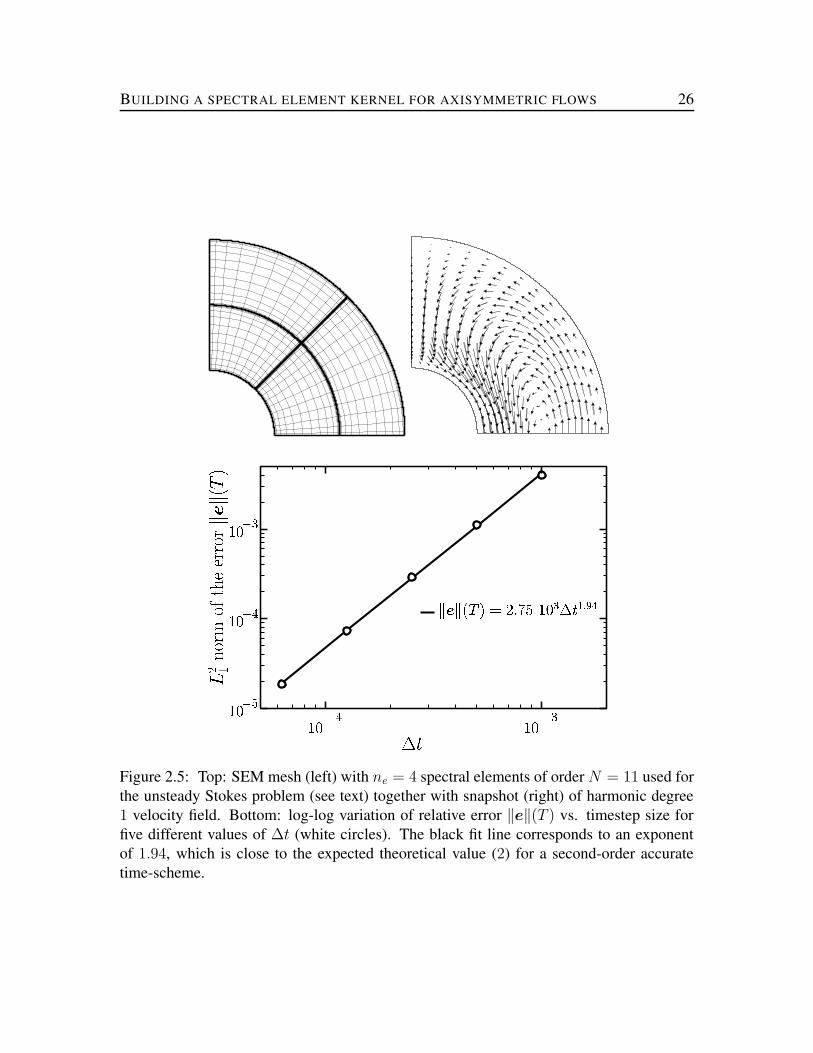
We repeat this procedure for various values of the timestep ∆t, and display the results in thebottom curve of figure 2.5. The error level (always above 10−5) is dominated by temporalerror, as expected. The largest ∆t has a value equal to τ/(10π), while smaller ∆ts follow ageometrical sequence of common ratio 1/2. The error level is proportional to the timestepsize with a power close enough to the expected value (1.94 vs 2) to confirm that neglectingthe residual term in equation (2.37) does not affect the overall order 2 accuracy of thetime-scheme.
BUILDING A SPECTRAL ELEMENT KERNEL FOR AXISYMMETRIC FLOWS 26
´µ·¶¸¹ º»¹¼ ½¾¿¿ ºº¹ ºÀDÁÀ  ÃÄ
ŦÆ
ÅÇÆ
ÅÇÈ
ÅÇÈÅÊÉ
ËSÌ
ËSÌ
ËSÌ ËSÌËSÌ Í3Î
Ï/ÐÊÏÒÑXÓ·Ô`Õ³Ö×ÙØÛÚ ËSÌÒÜ[ÝßÞ[àâá ãä
Figure 2.5: Top: SEM mesh (left) with ne = 4 spectral elements of order N = 11 used forthe unsteady Stokes problem (see text) together with snapshot (right) of harmonic degree1 velocity field. Bottom: log-log variation of relative error ‖e‖(T ) vs. timestep size forfive different values of ∆t (white circles). The black fit line corresponds to an exponentof 1.94, which is close to the expected theoretical value (2) for a second-order accuratetime-scheme.

BUILDING A SPECTRAL ELEMENT KERNEL FOR AXISYMMETRIC FLOWS 27
2.7 SEM vs. existing numerical solutions:The Proudman-Stewartson problem
2.7.1 Description
We conclude our presentation of the SEM by applying it to a simple flow problem morerelevant to geophysical situations. As shown in figure 2.6a, we consider a reference framerotating at a constant rate ω, where flow is induced inside a spherical shell by the superrotation of the inner sphere. We assume that the effects of rotation dominate the viscouseffects, which corresponds to E 1 in equation (2.1a). When the super rotation is smallenough, the solution is steady and axisymmetric (Proudman, 1956). Moreover, away fromviscous boundary layers, the velocity must obey the Taylor-Proudman theorem, i.e. it mustbe invariant along the axis of rotation:
∂zu = 0 . (2.55)
The Taylor-Proudman theorem leads to different flow regimes inside and outside of animaginary cylinder C, that circumscribes the inner sphere and is aligned parallel to the axisof rotation. This cylinder, commonly referred to as the tangent cylinder, is representedby a dotted line in figure 2.6a. Outside of C a fluid particle is insensitive to the superrotation of the inner sphere. It therefore stays at rest with respect to the background rotationω. Inside of C, however, a fluid particle senses the super rotation of the inner sphere,and is entrained in its direction. The background rotation induces via the Coriolis force ameridional circulation that is controlled by pumping and suction inside the viscous Ekmanboundary layers located at the inner and the outer shell boundaries (see figure 2.6a). Thecirculation is completed alongside of C, where a viscous shear layer (referred to as theStewartson layer) accommodates the angular velocity jump between regions inside andoutside C.
This classic kinematic flow problem in its asymptotic form was originally proposed byProudman (1956). It was developed later by Stewartson (1957; 1966), who derived theexact structure of the shear layers alongside of C. Since then it has been treated numeri-cally by several groups (Hollerbach, 1994; Dormy et al., 1998). In fact, though simple inessence, this so-called “Proudman-Stewartson Problem” exhibits the essential features offlows dominated by rotation. Its linear character, moreover, makes it an ideal test case toverify the numerical accuracy of our method, leaving aside complications that inevitablyappear when one introduces nonlinear effects. The Proudman-Stewartson problem is alsoquite challenging numerically, as one must resolve the narrow Ekman and Stewartson lay-ers that characterize the circulation when E 1.
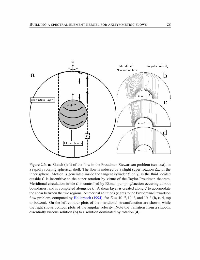
BUILDING A SPECTRAL ELEMENT KERNEL FOR AXISYMMETRIC FLOWS 28
å
åçæéèêå
ë
ìaíXîïð,ñGíòGó[ôöõ=ð÷[îñGò
øúùaû ð,ôüõ=ðâ÷#îñò
ý þÿ þ
#ÿ! "#$ þ&% #ÿ! "#$ þ&%' âÿ(
)
+*
, -
.
/
Figure 2.6: a: Sketch (left) of the flow in the Proudman-Stewartson problem (see text), ina rapidly rotating spherical shell. The flow is induced by a slight super rotation ∆ω of theinner sphere. Motion is generated inside the tangent cylinder C only, as the fluid locatedoutside C is insentitive to the super rotation by virtue of the Taylor-Proudman theorem.Meridional circulation inside C is controlled by Ekman pumping/suction occuring at bothboundaries, and is completed alongside C. A shear layer is created along C to accomodatethe shear between the two regions. Numerical solutions (right) to the Proudman-Stewartsonflow problem, computed by Hollerbach (1994), for E = 10−2, 10−3, and 10−4 (b, c, d, topto bottom). On the left contour plots of the meridional streamfunction are shown, whilethe right shows contour plots of the angular velocity. Note the transition from a smooth,essentially viscous solution (b) to a solution dominated by rotation (d).

BUILDING A SPECTRAL ELEMENT KERNEL FOR AXISYMMETRIC FLOWS 29
To summarize, we want to study numerically the following set of equations:
∂tu + 2z × u = −∇p + E∆u in Ω (2.56a)∇ · u = 0 in Ω (2.56b)
u(x, t) = sφ at r = ri (2.56c)u(x, t) = 0 at r = ro (2.56d)u(x, 0) = 0 in Ω , (2.56e)
for values of the Ekman number ranging from E = 10−2 to E = 10−4.
2.7.2 Reference numerical solution
We first describe the reference numerical solution together with the changes in the physicsof the solution, as we go from a slowly rotating system to a system rotating more rapidly.Our numerical reference solution is the spectral solution published by Hollerbach (1994).It is displayed in figure 2.6 for three values of E, 10−2 (figure 2.6b), 10−3 (figure 2.6c),and 10−4 (figure 2.6d). Hollerbach (1994) computed solutions to the steady problem, bysolving system (2.56) withdrawing the time-derivative in equation (2.56a). His spectralmethod satisfies the solenoidal constraint exactly, as the meridional circulation is describedin terms of a stream function, and in his approach the field variables are expanded by meansof Chebyshev and Legendre polynomials in the radial and angular direction, respectively.His published results include solutions for an Ekman number as low as 10−5. These resultswere subsequently confirmed by Dormy et al. (1998), who solved the Stewartson problemfor E as small as 2.37 10−8, using Legendre polynomials in the angular direction togetherwith a finite difference scheme in radius.
Looking at figure 2.6b, i.e. at the stream function and angular velocity of the flow atE = 10−2, we note that the solution is still essentially viscous and smooth. When E isdecreased by an order of magnitude (figure 2.6c), Ekman layers form in the vicinity of theshell boundaries. Away from these Ekman layers angular velocity contours and meridionalcirculation tend to align themselves with the axis of rotation, although the Taylor-Proudmantheorem is not fully satisfied as viscous effects are still noticeable. When we decrease Efurther to a value of E = 10−4, the Ekman layers sharpen significantly and the Stewartsonshear layer starts to develop (figure 2.6d, right). For this value of the Ekman number E,the circulation inside the tangent cylinder follows the Taylor-Proudman theorem quite well(figure 2.6d, left). This last case is the most challenging numerically.
2.7.3 SEM solution to the Proudman-Stewartson problem
We now turn our attention to the SEM solution of the Stewartson problem for the samethree Ekman numbers considered before. Our time-dependent calculations start with a

BUILDING A SPECTRAL ELEMENT KERNEL FOR AXISYMMETRIC FLOWS 30
Table 2.1: Summary of the Proudman-Stewartson problem results. Relative difference ‖d‖of SEM and spectral solution of Hollerbach (1994) for Ekman numbers 10−2, 10−3, and10−4. ne is the number of elements, N the polynomial order. Memory requirement isproportional to number of Gauss-Lobatto Legendre (GLL) points (Nnodes), while compu-tational cost scales approximately with neN
3. Note that ‖d‖ is in all cases well below theone per mil level.
E ne N Nnodes neN3 ‖d‖
10−2 4 11 529 5, 324 0.00000210−3 9 11 1, 156 10, 648 0.00016710−4 140 8 9, 153 71, 680 0.000119
fluid initially at rest. We then time-step our code until the flow settles to steady-state, andcompare this steady-state solution uh to the solutions obtained by Hollerbach. To computethe relative difference between the two numerical solutions:
‖d‖ =
(
∫
Ω(uh − us)
2dΩ∫
Ωu2
sdΩ
)1/2
, (2.57)
we project the purely spectral solution on the spectral element grid, and consider agreementbetween the two numerical approaches as acceptable at levels betters than ‖d‖ < 10−3.
The SEM results (angular velocity and meridional circulation) for E = 10−2, 10−3 and10−4 are displayed on the right-hand side of figure 2.7, and summarized in table 2.1. Recallthat unlike Hollerbach (1994), we do not describe the meridional circulation by means of astream-function in our method, and that we solve instead directly for the primitive variables(us, uz). We also show on the left-hand side of figure 2.7 the computational mesh used toobtain the solution.
For the large Ekman number case (E = 10−2, figures 2.7a/b/c) 4 spectral elements areneeded to retrieve the solution. Setting the polynomial order to 11 leads by virtue of thespectral convergence properties of the SEM (see section 2.6.1) to excellent agreement withHollerbach’s solution, as the relative difference between the two methods for this smoothsolution is ‖d‖ = 0.000002. For the medium and low Ekman number cases (E = 10−3
and E = 10−4, figures 2.7d/e/f and figures 2.7g/h/i), we reproduce Hollerbach’s solutionwith our required level of accuracy (‖d‖ < 10−3) at the expense of an increased numericalresolution (see table 2.1). In the latter case, we use 140 elements of polynomial order 8 (seefigure 2.7g). These elements are gently squeezed toward the boundaries of the shell. If onewere to squeeze them further, the contrast in aspect ratio between neighboring elementsand the resulting anisotropy in the computational mesh would lead to a deterioration ofcondition in the algebraic system (2.39), and thus to a larger computational cost. We do notconsider smaller Ekman number solutions here, because their computational requirements(integration time and computer memory) would be prohibitive for single processor runs
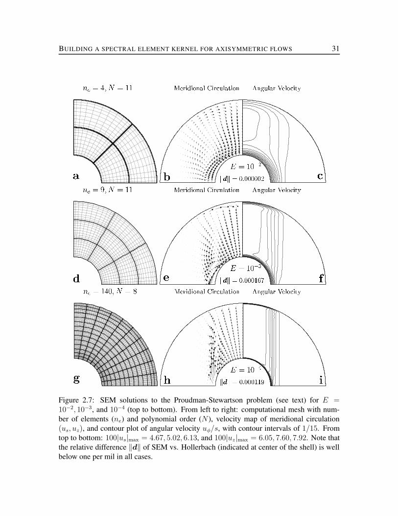
BUILDING A SPECTRAL ELEMENT KERNEL FOR AXISYMMETRIC FLOWS 31
Non-axisymmetric Mesh 02143 57698:<;>=6?@ACBEDF =:#AGHA9?1786JIKA:#@5H6L8MB#A9?1NKOQPSRTVUXWYZP\[
]_^a`bVcJdefgeihkj4lmjjjHnnop q r
Non-axisymmetric Mesh s2t4u+vHw9xy<z|w~C y#H9t7xwX<y#~vHw9x#9tiQ\Xa7
S"Xgik4H
2¡4¢+£H¤9¥¦<§|¨¤©ª«C¬® ¨¦#«¯H«9©¡7¥¤X°<«¦#ª£H¤9¥¬#«9©¡±i²Q³µ´·¶¸³a¹7¹
º»S¼½"¾À¿ÁÂgÁiÃkÄ4ÅÄÄÄÄÄ ÆÇ È É
Figure 2.7: SEM solutions to the Proudman-Stewartson problem (see text) for E =10−2, 10−3, and 10−4 (top to bottom). From left to right: computational mesh with num-ber of elements (ne) and polynomial order (N ), velocity map of meridional circulation(us, uz), and contour plot of angular velocity uφ/s, with contour intervals of 1/15. Fromtop to bottom: 100|us|max = 4.67, 5.02, 6.13, and 100|uz|max = 6.05, 7.60, 7.92. Note thatthe relative difference ‖d‖ of SEM vs. Hollerbach (indicated at center of the shell) is wellbelow one per mil in all cases.

BUILDING A SPECTRAL ELEMENT KERNEL FOR AXISYMMETRIC FLOWS 32
ÊËÌÍÎÏÑÐËÒ ÏÓ ËÊË ÔÕËÖ ×Ö
Ø Ù Ú Û Ü Ý Þ+ßàÞVÞáÞ+â
ãä2åäiæäKçä<èäiéäKê
Þ+ßÞ ßÞ ßÞ ßÞ ßÞ ßÞ ß ë
ìÀíÑî<ïiì!ðòñóJíôì!õöi÷7õáøFigure 2.8: Relative difference ‖d‖ of SEM vs. Hollerbach(1994) spectral solution toProudman-Stewartson problem (see text) for E = 10−3 as function of polynomial orderN for computational mesh with and without grid-refinement, as indicated by inlet-figures.The mesh with uniform resolution consists of ne = 4 spectral elements, while the non-uniform mesh includes ne = 16 elements, concentrated in Ekman layers at both shellboundaries. The ne = 16 mesh (bottom curve) shows lower overall difference, as expected,due to its larger number of elements. Note, however, that this mesh is characterized byspectral convergence up to the highest polynomial order (N = 12) employed, while theuniform resolution mesh (top curve) shows a flattening of the convergence, indicating thatmesh-refinement is well suited to describe the Ekman layers and results in an overall fasterconvergence rate.
using standard personal computers. However, we are currently parallelizing our code toenable computations at lower Ekman numbers.
2.7.4 Adaptivity and enhanced convergence
We complete our study of the SEM by examining its potential for grid-refinement. Indeed,the local character of the SEM allows for a non-uniform paving of the domain. We madeuse of this property in our study of the Stewartson problem by radially squeezing spectralelements in the vicinity of the Ekman boundary layers. More generally, the adaptivityof grid-based methods, such as the SEM, is well suited to capture strong gradients byproviding increased numerical solution in regions containing fine-scale structures.
To illustrate this property in a quantitative way, we consider the solution of the Stewartson

BUILDING A SPECTRAL ELEMENT KERNEL FOR AXISYMMETRIC FLOWS 33
problem at E = 10−3 obtained with two different meshes (portrayed in figure 2.8) for anumber of polynomial orders N . As we have seen before, the value of E in this interme-diate case is small enough to permit the development of strong Ekman layers. We wantto quantify how well we succeed in describing these localized features of the Proudman-Stewartson solution by using either an almost uniform mesh of ne = 4 elements, or a non-uniform mesh having ne = 16 spectral elements where the exterior elements are squeezedby a factor of three relative to interior elements. We expect, for the same polynomial orderN , that our mesh with local grid-refinement should yield better results than our mesh ofalmost uniform grid resolution due to its larger number of elements. But, more importantly,we also expect that our ability to adapt the mesh geometry to conform to the inherent flowstructure, with narrow Ekman layers concentrated near the shell boundaries, should fur-thermore lead to a faster convergence rate when we increase the polynomial order. Thisbehaviour is indeed confirmed by the two curves in figure 2.8 showing the accuracy of oursolution as a function of the polynomial order N . The top curve (for the uniform mesh)tends to flatten as we increase the polynomial order above 10, while the bottom curve (forthe non-uniform mesh) does not show any sign of flattening.
2.8 Discussion
In this paper we have presented the application of the spectral element method to modelaxisymmetric flows in a rapidly rotating reference frame. Spatial discretization relies onbreaking the physical domain into a collection of ne non-overlapping elements, and us-ing a local tensorized basis of polynomials of high order N . The temporal discretizationis achieved by means of a second-order accurate backward differentiation scheme for thetime-derivative, and we follow an operator integrated factor (OIF) approach to treat theresulting modified Stokes problem at each timestep. Our use of the OIF strategy is mo-tivated by the fact that the mass matrix arising from the spatial discretization is diagonal.Our implementation of the OIF, relative to a standard implementation of the OIF (Madayet al., 1990) where only viscous effects are treated, is modified such as to account for theeffects of the Coriolis force. Hence both viscous and Coriolis effects are treated fully im-plicitly in our approach. The computation of the pressure increment is accomplished usingan efficient additive overlapping Schwarz preconditioner.
We have validated our implementation of the method by comparing it to analytical and pub-lished spectral reference solutions of axisymmetric laminar flows in a spherical shell. Oursteady-state analytical benchmark solutions demonstrate that no spurious pressure modeexists due to the discretization of the pressure using a lower polynomial order (N − 2)relative to the polynomial order (N ) that is used for the velocity. The PN −PN−2 approachfor velocity and pressure therefore guarantees the solenoidal character of the velocity field.These results furthermore served to demonstrate the spectral convergence properties of theSEM. The unsteady analytic benchmark solution allowed us finally to verify that the rela-

BUILDING A SPECTRAL ELEMENT KERNEL FOR AXISYMMETRIC FLOWS 34
tively unusual time discretization strategy adopted here is second-order accurate.
We have used published spectral solutions to the kinematic Proudman-Stewartson problem(Hollerbach, 1994) at Ekman numbers of 10−2, 10−3, and 10−4 to assess the efficacy ofthe SEM in a rapidly rotating context. These solutions, which exhibit some of the essentialfeatures of flows dominated by rotation, confirm consistency between the two differentnumerical techniques at levels of better than one per mil. In fact, our calculations forthe Stewartson problem demonstrate for all practical purpose that the SEM solutions areidentical to the solution published by Hollerbach. This close correspondence between SEMand spectral solution shows that our inclusion into the SEM of the effects of a dominantCoriolis force, a relatively novel extension to standard applications of the SEM, does notaffect the overall accuracy of the method.
We have shown that the local character of the SEM is well suited for a non-uniform pavingof the computational domain, i.e. for grid-refinement in regions of the flow characterizedby strong local gradients such as Ekman boundary layers at the Core Mantle Boundary(CMB) and the Inner Core Boundary (ICB). In fact, exploiting mesh-refinement in theresolution of the Proudman-Stewartson problem leads to a substantial improvement in theconvergence properties of the method. Given the high numerical accuracy of the SEM, itslocal and hence inherently parallel character, as well as its adaptivity, these early results areencouraging in the long-term prospect of building a parallel spectral element based modelof the geodynamo.
The extension of the present kernel to 3-D problems can be achieved through a mixedFourier-spectral element approach (Bernardi et al., 1999), where the longitudinal depen-dence of the variables is expanded into Fourier series. The approach, effectively, breaks the3-D problem into a set of meridional problems quite similar to the ones presented in thispaper. The special treatment of spectral elements adjacent to the axis of rotation we intro-duced is well suited for this technique. Moreover, the Schwarz preconditioner we use hereto compute the pressure increment at each timestep lends itself naturally to computationallydemanding problems in 3-D applications.
The local character of the SEM allows for a straightforward spatial domain decompositionin the meridional plane using active message-passing to communicate among subdomains,i.e. for inter processor communication. The strategy is illustrated in figure 2.9, where weshow an example of a 3-D mesh, color-scale coded for parallelization among processors.This approach should allow us to take advantage in the future of the gain in computationalspeed on modern parallel computers.
Our method should carry over to the implementation of the magnetic component of the geo-dynamo problem. For example, imposing the divergence-free constraint on the magneticfield B can be accomplished using the same approach we used to enforce the divergence-free constraint on the velocity field u. Likewise, accounting for the effects of the inner core(Hollerbach & Jones, 1993) can be accomplished by extending our computational domain

BUILDING A SPECTRAL ELEMENT KERNEL FOR AXISYMMETRIC FLOWS 35
Figure 2.9: 3-D spherical mesh for mixed Fourier-spectral element approach (see text).The mesh consists of 32 spectral elements in the meridional plane together with 32 equallyspaced points in longitude. The spatial domain decomposition (indicated by color-scale)for parallel processing is illustrated for 16 processors handling 2 spectral elements each.
beyond the ICB radially inwards to include the solid inner core. The main complexity re-lated to the magnetic induction equation lies in imposing the magnetic boundary conditionsat the CMB, where the magnetic field has to be connected to an exterior potential field. Thismatching condition translates to an elegant analytic boundary condition in the context ofspherical harmonics (Glatzmaier, 1984). It is, however, less amenable to a local method,and it is yet to find out how this matching is to be accomplished. An alternative to thismatching has been presented by Chan et al. (2001), who meshed the external space up to afew core radii and used approximate magnetic boundary conditions on the outer surface ofthe computational domain. We are currently investigating different strategies regarding theimplementation of the induction equation and we hope to benefit, in a nonlinear context,from the weak numerical dispersion of the SEM.

Chapter 3
A Fourier-spectral element algorithm forthermal convection in rotatingaxisymmetric containers
3.1 Introduction
Large-scale planetary fluid flows are strongly influenced by the background rotation ofplanetary bodies. On Earth, the effects of the Coriolis force in the atmosphere and inthe oceans are observed (and monitored) on an hourly basis. At the same time, geologicalrecords of the magnetic field of the Earth (generated inside its liquid iron outer core throughdynamo action) indicate that the geomagnetic field is on average parallel (or anti-parallel)to the North-South axis (Merrill et al., 1996). Each terrestrial fluid layer is therefore verysensitive on its own timescales to the Earth’s rotation ω. This reflects the importance of theso-called geostrophic equilibrium, in which the Coriolis force 2ρω ×u (where ρ and u arethe fluid density and velocity, respectively) is balanced by the pressure gradient ∇p :
2ρω × u = −∇p. (3.1)
Taking the curl of this balance leads to
2ω(z∇ · u − ∂zu) =1
ρ∇ρ ×∇p, (3.2)
where z is the unit vector in the direction of rotation (ω = ωz ). Throughout this paper,(x, y, z), (s, φ, z), and (r, θ, φ) will denote Cartesian, cylindrical, and spherical coordinates,respectively.
If we further assume that the fluid has a constant density ρ = ρ0, we obtain the so-calledTaylor-Proudman theorem
∂zu = 0. (3.3)
36
EXTENDING THE KERNEL TO THREE-DIMENSIONAL CONVECTIVE FLOWS 37
This theorem implies that a fast rotation introduces a substantial amount of anisotropy inthe flow, which tends to be invariant along the direction of rotation; the flow is organizedin a columnar fashion, the columns being parallel to the z-axis.
Deviations from a geostrophic state arise from the (re)introduction of other dynamical in-gredients in the momentum equation. Viscous forces are for instance required if no-slipboundary conditions are to be applied. They are responsible for the generation of sharpEkman boundary layers, in which there is a local equilibrium between the Coriolis force,the pressure gradient and the viscous force. Moreover, inertia induces the existence of aclass of fast oscillations called inertial waves, the frequency of which is smaller than 2ω(Greenspan, 1990). A departure from a geostrophic equilibrium can also occur when a largeenough body force is applied to the fluid. For instance, thermal heterogeneities in a vis-cous fluid can drive non-geostrophic motion. In a classical paper, Busse (1970) showed thatthermal instabilities in a sphere took the form of a drifting sequence of narrow columns par-allel to the axis of rotation. In particular, he demonstrated that the critical longitudinal wavenumber kc characterizing this “banana belt” instability varies in the rapidly rotating limitas ω1/3: the larger the rotation rate, the smaller the equatorial extent of the so-called Bussecolumns. On a similar note, in the case of metallic planetary cores, this body force canbe the Lorentz force, the feedback from the magnetic field on the fluid flow. The balancebetween Coriolis force, pressure force, and the Lorentz force is called the magnetostrophicbalance (Gubbins & Roberts, 1987).
Having in mind on the long run to design a model able to simulate flows in planetary cores,our objective in this paper is to present a numerical formulation to solve thermal convectionfor a neutral viscous fluid, in the framework of the Boussinesq approximation and in therapidly rotating limit.
Because of its relevance for planetary and stellar studies, this problem has received con-siderable attention from modelers over the past thirty years, and we begin by a review ofthe different methods that have been used to address it. The most successful attempts fornumerical simulations of geophysical flows in rotating spherical shells to date are basedupon spectral transform methods (STM) which expand the variables of interest on thetwo-sphere upon the global basis of spherical harmonics, while Chebyshev collocation orfinite-differences are generally used in radius (Glatzmaier, 1984; Kuang & Bloxham, 1999;Tilgner, 1999; Hollerbach, 2000; Christensen et al., 2001). Time integration is performedin spectral space using a Courant limited numerical time step, and nonlinear terms are com-puted at each time step by transforming functions back into grid space (typically a latitude-longitude structured grid), in which nonlinear products are computed. Spherical harmonicsare remarkably accurate and stable for smooth flows and allow for a completely isotropicrepresentation of scalar functions: they provide a uniform resolution on the two-sphere andare not biased toward the poles (Boyd, 2001). This allows the horizontal Courant conditionto be based on an average horizontal resolution, related to the highest spherical harmonicdegree L, the vertical Courant condition being controlled by the vertical discretization cho-sen.

EXTENDING THE KERNEL TO THREE-DIMENSIONAL CONVECTIVE FLOWS 38
A large body of work has grown, addressing the problem of efficient and stable compu-tation of scalar spherical harmonic transforms (Orszag, 1974; Alpert & Rokhlin, 1991;Swarztrauber & Spotz, 2000), as well as of harmonic transforms for vector and tensorfields on the two-sphere (Swartztrauber, 1993; Kostelec et al., 2000). However, STM stillsuffer from some drawbacks :
1. the need for high-order truncations when the flow develops non smooth and spatiallylocalized small-scale features;
2. their restriction to spherical geometry. Aspherical geometrical features can be intro-duced only through a perturbative approach (assuming therefore a small deviationfrom sphericity) or an involved coordinate transform –to model for instance flows inspheroidal shells (Lorenzani & Tilgner, 2001);
3. the difficulty to incorporate mesh refinement;
4. more specifically, in the rapidly rotating limit, the implicit treatment of the Coriolisforce, which allows to control inertial waves, couples spherical harmonics coeffi-cients and has a severe impact on memory requirements (Hollerbach, 2000);
5. their difficulty to parallelize efficiently due to communication overheads.
This last issue arises from the fact that spherical harmonics are tensor products of combina-tions of Fourier series in longitude with associated Legendre functions in latitude. Despiterecent improvements, no fast discrete spherical transform exists and the transform requiresO(L3) operations (Spotz & Swarztrauber, 2001). This corresponds to a computational ef-fort of O(L4) in three dimensions, assuming that roughly the same resolution is adopted inthe vertical direction as on the two-sphere. At high resolution, the transforms become themain part of the computations –more than 80% of the total CPU in Kuang and Bloxham’sthree-dimensional (3D) dynamo model (Kuang & Bloxham, 1999). On distributed mem-ory architectures, the global nature of the STM imposes overhead in the communicationsbetween processors that becomes critical as L increases. We should mention, however, arecent and successful effort by Clune et al. (1999) who developed a highly efficient parallelimplementation on the CRAY T3E of a STM code originally written by Glatzmaier (1984).
Aside from STM approaches, a growing number of studies have been conducted towardgrid-based numerical methods in spherical geometries. Most of them are based upon finitedifferences (FD) (Kageyama et al., 1993; Gilman & Miller, 1986) or pseudo-spectral (Forn-berg, 1995) methods formulated in cylindrical or spherical coordinates. FD methods arepenalized by grid dispersion near strong gradients and require a large number of grid pointsto achieve the expected accuracy. Higher-order methods, like pseudo-spectral methods, areable to reach the expected accuracy using fewer grid points (Fornberg & Merrill, 1997).These methods are nevertheless based on the strong form of the equations and face severelimitations for an accurate approximation of Neumann boundary conditions. The major

EXTENDING THE KERNEL TO THREE-DIMENSIONAL CONVECTIVE FLOWS 39
problem of these methods is that they fail to provide a uniform representation of scalarfunctions on the two-sphere. Latitude-longitude grids are indeed highly non-isotropic witha clustering of points near the poles that leads to severe timestep restrictions (Boyd, 2001,§ 18.10). The pole singularity requires special treatment like the reformulation of the gov-erning equations or the use of staggered grid strategies. These methods have neverthelesssome advantages, not only in terms of storage and periodicity, but also in terms of efficientcalculation of spatial derivatives on the two-sphere that take advantage of the structure ofa latitude-longitude grid. One such approach, previously proposed by Merilees (1973),which uses fast Fourier transforms (FFT) on circles on the sphere, has been recently re-visited by Fornberg (1995), and Spotz et al. (1998) and shown to be quite accurate whenused in conjunction with suitable spectral filters (Jakob-Chien & Alpert, 1997; Yarvin &Rokhlin, 1998). It has been applied to the shallow water equations, and remains to be ex-plored in the context of planetary cores dynamics, for which the thin shell approximationis no longer valid. A way to circumvent the pole problems associated with the sphericalor cylindrical coordinates systems is to resort to Cartesian coordinates and multidomaindecomposition (Sadourny, 1972; Rancic et al., 1996; Ronchi et al., 1996). In this case, oneis still facing the non trivial problem of gluing together different coordinate systems. Thisgenerally implies overlapping regions between mesh subdomains, which puts new stabilityconditions and new complexities into the implementation.
Other promising grid-based methods stem from the variational formulation of the momen-tum and energy equations and include the finite element method (FEM) and the spectralelement method (SEM), using spherical geodesic grids generated either from the tiling ofan icosahedron (Sadourny et al., 1968; Baumgardner & Frederikson, 1985; Giraldo, 2001;Matsui & Okuda, 2002) or a gnomic projection (Sadourny, 1972; Ronchi et al., 1996; Tay-lor et al., 1997; Giraldo et al., 2003). In the latter case, the two-sphere is decomposed intosix regions which are isomorphic to the six faces of a cube. A spherical grid can be obtainedby projecting, using the central gnomic projection, a quadrangular mesh of the surface ofthe cube into its circumscribed sphere. As a result of the gnomic projection, any straightline drawn on a face of the cube is transformed into a geodesic on the sphere. The 3D meshof a spherical shell is then obtained by radially connecting the quadrangles between twoconcentric cubed spheres. The discretization of the whole sphere can then be completed ifneeded by inscribing a cube at the center with a smooth transition (Chaljub et al., 2003).Such a discretization provides a uniform tilling of the two-sphere avoiding classical poleproblems of spherical and cylindrical coordinates and the singularity at the center of thesphere is naturally removed. All the transformations involved are analytical and can beadjusted to account for ellipticity or surface topography. Thanks to the variational formula-tion, the FEM and SEM provide a natural setting for handling the connection between thesix domains produced by the central projection. They also allow for local mesh refinementusing elements of variable sizes which can be conforming or nonconforming (Bernardiet al., 1994; Levin et al., 2000; Chaljub et al., 2003).
The SEM is specifically quite appealing: it has now become customary to highlight that itcombines the geometrical flexibility of conventional finite element methods with the expo-

EXTENDING THE KERNEL TO THREE-DIMENSIONAL CONVECTIVE FLOWS 40
nential convergence rate associated with spectral techniques (Orszag, 1980). In each ele-ment, spatial discretization is based upon Legendre polynomials which, together with theuse of a Gauss-Lobatto quadrature, leads to a diagonal mass matrix. Moreover, the SEMretains the efficiency of sum-factorization techniques thanks to a tensorized formulation(Patera, 1984; Bernardi & Maday, 1992; Ma, 1993). Communications between elementsare local and only require the exchange of boundary informations between neighbors. Effi-cient parallelization can be achieved on distributed memory architecture and excellent scal-ings have been measured as far as explicit time schemes are involved (Iskandarani et al.,2003). The SEM yields a O(neN
d+1) complexity, where ne is the number of elements,N refers here to the polynomial degree used in each direction inside each element, and dis the number of spatial dimensions. Since the ratio of the number of elements ne to Ncan be controlled, N is generally much smaller than the maximum degree L of sphericalharmonics in STM models and the cost of the transforms is kept in line with the rest of themodel. The SEM has the disadvantage, though, that it gives rise to linear operators whichare difficult to invert if one uses semi-implicit or fully implicit schemes (essential in therapidly rotating limit). This statement is particularly relevant for the elliptic operator thatmust be inverted to compute the pressure increment in pressure correction schemes. Iter-ative methods with efficient preconditioners are required that permit an efficient parallelimplementation. This is not a trivial task, especially in three dimensions (Fischer et al.,2000).
The main purpose of this paper is to introduce and validate an efficient and accurate implicitand semi-implicit grid-based method to simulate convection in rotating spherical or ellip-soidal geometries. Such a method must meet several requirements in order to be adaptedto the dynamics of planetary cores:
1. an accurate discretization of spherical or ellipsoidal geometries;
2. a natural approximation of surface boundary and interface continuity conditions;
3. an expansion of the physical variables upon bases with local support;
4. a natural setting for local mesh refinement in order to capture small scale features ofthe 3D flow and especially boundary layers;
5. a minimal numerical dispersion;
6. an accurate solution for pressure;
7. an efficient parallel implementation on distributed memory architectures.
We choose to resort to the SEM, which appears to be the best candidate to fulfill these con-ditions. At the same time, in order to keep the numerical complexity of the problem as lowas possible, we set the problem in cylindrical coordinates (the set of coordinates naturallyassociated with the Taylor-Proudman theorem) and make use of the 2π natural periodicity

EXTENDING THE KERNEL TO THREE-DIMENSIONAL CONVECTIVE FLOWS 41
in longitude for spherical and ellipsoidal geometries, by expanding the physical variablesin Fourier series in φ. This leads to a finite number of K+1 coupled two-dimensional prob-lems written in the meridional plane, where K is the highest Fourier angular mode retainedin the expansion. These problems are coupled only through the nonlinear terms, whileno extra coupling arises from the linear rotation (Coriolis) term, since the axis of rotationdoes coincide with the z-axis of the cylindrical coordinates set. Such a method, hereafterreferred to as the Fourier-spectral element method (FSEM), provides substantial simplifi-cations in terms of implementation and mesh design, thanks to the dimension reduction andthe elimination of the angular curvature. Let us stress here that the methodology presentedin this paper is valid for any kind of 3D domain with axial symmetry.
A brief description of the governing equations in the 3D domain is provided in section 3.2,and their standard variational formulation is given for reference in section 3.3. In sec-tion 3.4, we reformulate the problem in cylindrical coordinates and reduce its dimension byperforming a Fourier expansion in longitude. Because of this Fourier reduction, functionswhich belong to standard Sobolev spaces in the three-dimensional domain are mapped ontofunctions which belong to weighted Sobolev spaces in the meridional domain, the weightbeing the distance to the axis of symmetry. The discretization must rely on a well-posedvariational formulation in the natural spaces in which the Fourier coefficients lie which areprecisely these weighted Sobolev spaces (Bernardi et al., 1999).
The main issue related to the implementation of the meridional discretization arises fromthe so-called pole conditions linked to the singularity of the polar transformation at thesymmetry axis (Boyd, 2001). In section 3.5, these pole conditions are reviewed and thedistinction between essential and natural axial conditions, which must be met by the phys-ical fields in the meridional plane, is introduced following Tomboulides (1993) and Lopezet al. (2002). Natural axial conditions need to be enforced ab initio in the definition ofthe weighted Sobolev spaces of the variational formulation while essential axial conditionshave to be imposed in order for the variational formulation to be well-posed. FollowingBernardi et al. (1999), we introduce consequently the appropriate weighted Sobolev spacesand the variational formulation of the various meridional problems.
In section 3.6, we describe the extensions required for the standard SEM to handle boththe Fourier discretization with respect to the angular variable (longitude) and the weightedmeasure. As stated above, the standard SEM relies on an approximation by high order ten-sorized orthogonal polynomial bases and Gauss-type quadratures. However, the weightsinduced by the axisymmetric reduction are not standard, i.e. they (or their inverse) arenot integrable, and, in the FSEM, polynomial approximation and quadrature formulas haveto be revisited for any element adjacent to the symmetry axis. The choice of the quadra-ture formula is not so obvious (Bernardi et al., 1999): in particular, it must involve axialboundary nodes in order to enforce essential pole conditions, with the help of l’Hospitalrule to remove apparent singularities. This is accomplished here by introducing a weightedGauss-Lobatto-Legendre quadrature. Another important aspect is related to the divergence-free discrete velocities in the Boussinesq approximation. Following Bernardi and Maday

EXTENDING THE KERNEL TO THREE-DIMENSIONAL CONVECTIVE FLOWS 42
(1988), velocity and pressure are approximated by polynomials of different order, i.e. thepressure involves a lower order polynomial approximation. This allows us to derive thesemi-discrete formulation of the rotating convection problem.
In section 3.7, we describe in detail the time discretization and the fractional step methodused to advance the model in time. In order to solve the time dependent problem efficiently,it is a general practice for spectral approximations to treat nonlinear terms explicitly and weresort here to a third-order Adams-Bashforth approximation. In the rapidly rotating limit,we have seen that our interest lies in treating both viscous and Coriolis terms implicitly(Hollerbach, 2000). For this specific situation, we introduce a second-order backward dif-ferentiation in time for partial time derivatives. Otherwise, we use a semi-implicit schemewith a simple mid-point approximation for the viscous and Coriolis terms. Whichever op-tion we retain, we still face the difficulty associated with the divergence-free constraint aris-ing from the Boussinesq approximation, which couples the discrete pressure and velocityfields. An efficient way to circumvent this coupling is to use a fractional step (projection)method (Chorin, 1968). As advocated by Perot (1993), the splitting is done at the algebraiclevel, and any reference to boundary conditions for pressure is bypassed, thereby avoid-ing the generation of divergence boundary layers. Following original studies by Maday etal. (1993), Couzy (1995) and Fischer (1997), we derive a stable second-order projectionscheme that involves at the projection step the inversion of a poorly conditioned symmetricpseudo-Laplacian operator. This inversion is performed iteratively, using a preconditionedconjugate gradient algorithm based upon the overlapping Schwarz method introduced byFischer (1997, and references therein), and adapted to axisymmetric problems by Fournieret al. (2003a).
Finally, in section 3.8, we present three sets of numerical comparisons with analyticaland/or numerical solutions in spherical and cylindrical geometries. In all cases, the numer-ical results demonstrate the accuracy and the convergence of the FSEM. We end the paperwith some concluding remarks and perspectives, and provide in the appendices details onthe weighted Gauss-Lobatto-Legendre quadrature and on the removal of the apparent axialsingularities.
3.2 Governing equations
Consider a homogeneous Newtonian convecting fluid of density ρ, kinematic viscosity νand thermal diffusivity κ, embedded in an axially symmetric container Ω which can berotating about its axis of symmetry at a constant rate ω (see figure 3.1). Let z denotethe unit vector in the direction of rotation. We assume that motion is driven by thermalanomalies only and choose the following length and time scales:
[L] ∼ a, [t] ∼ a2/ν, (3.4)

EXTENDING THE KERNEL TO THREE-DIMENSIONAL CONVECTIVE FLOWS 43
Ω
×
z
x y
sφ
-z
r
ω
Γ Ω
∂Ω
Figure 3.1: The three-dimensional domain Ω (in this example an oblate spheroid) is axiallysymmetric about the axis Γ and can rotate about this axis at a rate ω. We denote the merid-ional section of Ω with Ω, and its meridional boundary with ∂ Ω. Cylindrical coordinatesare denoted with (s, φ, z), with the z axis aligned with the axis of symmetry.
in which a is a typical dimension of the container. Accordingly, ν/a and ρν2/a2 are thevelocity and pressure scales.
In the framework of the Boussinesq approximation (Chandrasekhar, 1961), the nondimen-sional conservations of mass, momentum and energy write respectively
∇ · u = 0, (3.5a)∂tu + u · ∇u + 2C z × u + ∇P = ∇2u + f(T ), (3.5b)
∂tT + u · ∇T =1
Pr∇2T − u · ∇Ts, (3.5c)
where u is the fluid velocity, P is the pressure perturbation, T is the temperature anomaly,and Ts is the static (conductive) temperature distribution. We assume that this set of equa-tions is supplemented by suitable initial conditions and by homogeneous Dirichlet bound-ary conditions for velocity and temperature anomaly on the boundary of the container ∂ Ω.These correspond physically to no-slip conditions for fluid flow and an imposed tempera-ture on ∂ Ω. Note that the implementation of stress-free and thermally insulating boundaryconditions require only slight modifications of the implementation described in what fol-lows.
The Coriolis number
C =a2ω
ν(3.6)
expresses the relative importance of rotational versus viscous effects. It is the inverse ofthe Ekman number
E =ν
a2ω, (3.7)

EXTENDING THE KERNEL TO THREE-DIMENSIONAL CONVECTIVE FLOWS 44
the use of which is more frequent in geophysical fluid dynamics (Greenspan, 1990). Therapidly rotating limit we mentioned in the introduction corresponds to C 1, or equiva-lently, E 1.
The explicit expression of f in equation (3.5b) depends on the problem of interest. It istypically of the form
f(T ) = −RT g, (3.8)
in which g is the unit vector parallel to the gravity field and R is the (nondimensional)Rayleigh number. The Rayleigh number is a measure of the vigor of convection and itsexpression depends on the physical properties of the fluid of interest (thermal diffusivity,coefficient of thermal expansion, kinematic viscosity), on the strength of gravity, and onthe thermal scale chosen. This thermal scale is related to the basic (conductive) thermalstate Ts which depends in turn on the thermal boundary conditions, and on the presence ofinternal heat sources hs. For the sake of clarity, we will ignore these subtleties throughoutthe discussion of the numerical method. We shall, however, provide explicit expressionsfor f(T ) and R when dealing with the examples of section 3.8.
Finally, Pr in equation (3.5c) is the Prandtl number
Pr =ν
κ, (3.9)
the ratio of viscous diffusivity to thermal diffusivity. Values of Pr include Pr = 6.7 forwater and Pr = 0.02 for liquid metals.
3.3 Three-dimensional weak form
It might be useful at this early stage to recall quickly the weak formulation associatedwith the original three-dimensional problem (3.5). After introducing the space of squareintegrable functions
L2(Ω) =
w : Ω → R,
√
∫
Ω
w2d Ω < +∞
, (3.10)
in which d Ω = dxdydz, we define the Sobolev space H1(Ω) of those functions of L2(Ω)whose first partial derivatives are also in L2(Ω)
H1(Ω) =
w ∈ L2(Ω); ∂iw ∈ L2(Ω), i = 1, 2, 3
, (3.11)
in which i = 1, 2, 3 denotes the (x, y, z) Cartesian coordinates, respectively. Furthermore,we define H1(Ω) as the space of vectors whose components belong to H1(Ω). The fact

EXTENDING THE KERNEL TO THREE-DIMENSIONAL CONVECTIVE FLOWS 45
that both velocity and temperature satisfy homogeneous boundary conditions prompts usto define
H1(Ω) =
w ∈ H1(Ω), w = 0 on ∂ Ω
, (3.12)
and its vectorial extension
H1(Ω) =
w ∈ H1(Ω),w = 0 on ∂ Ω
. (3.13)
With this catalog of functional spaces at hand, we can write the weak form associated withproblem (3.5):
Find (u, P, T ) in H1(Ω) × L2(Ω) × H1(Ω), such that
∀q ∈ L2(Ω), −d(u, q) = 0, (3.14a)
∀w ∈ H1(Ω), (w, ∂tu) + 2Cc(w,u) − d(w, P ) + a(w,u) = (w,b), (3.14b)
∀v ∈ H1(Ω), (v, ∂tT ) +1
Pra(v, T ) = (v, bT ), (3.14c)
whereb = f − u · ∇u, bT = −u · ∇(T + Ts), (3.15)
and
(v, T ) =
∫
Ω
vTd Ω (3.16)
is the inner product for scalar functions,
(w,u) = (wi, ui) (3.17)
is its three-dimensional extension,
c(w,u) = −(w1, u2) + (w2, u1) (3.18)
is the Coriolis form,
d(u, q) = (∇ · u, q) (3.19)
is the divergence-pressure form,
a(v, T ) = (∇v,∇T ) (3.20)
is the scalar gradient form and
a(w,u) = a(wi, ui) (3.21)
EXTENDING THE KERNEL TO THREE-DIMENSIONAL CONVECTIVE FLOWS 46
is the vectorial gradient form. Variants of this variational problem have received consider-able attention over the past decades, due to its relevance for heat transfer (see e.g. Reddy,1993). In particular, equations (3.14a) and (3.14b) define an unsteady Navier-Stokes prob-lem (modified here by the effects of the background rotation through the Coriolis form c).The time discretization of such a problem leads to a modified Stokes problem to solve ateach timestep (Fischer, 1997). Such a saddle-point problem admits a unique solutions upto an additive constant for pressure, provided that pressure and velocity are approximatedin spaces that disallow the existence of spurious pressure modes (see e.g. Deville et al.,2002, chap. 6, and references therein).
3.4 Strong cylindrical form - Problem reductionby a Fourier expansion in longitude
The variational formulation we just described is the foundation upon which the spectralelement method can be subsequently built, through the tiling of the three-dimensional do-main in a collection of non-overlapping elements (Rønquist, 1988). In our case, however,the axisymmetry of Ω, as well as the Proudman-Taylor theorem (3.3) in the rapidly rotatingsituation, favors the use of a (s, φ, z) system of cylindrical coordinates (see figure 3.1). Thedependence in φ can then be accounted for through a Fourier expansion, which breaks theoriginal three-dimensional problem in a collection of two-dimensional ones.
Firstly, let us switch from Cartesian to cylindrical coordinates. If (us, uφ, uz) denote thethree cylindrical components of velocity, then set (3.5) can be equivalently written as
∂sus +1
sus +
1
s∂φuφ + ∂zuz = 0, (3.22a)
∂tus − 2Cuφ + ∂sP = ∇2us −us
s2− 2
s2∂φuφ + bs, (3.22b)
∂tuφ + 2Cus +∂φP
s= ∇2uφ − uφ
s2+
2
s2∂φus + bφ, (3.22c)
∂tuz + ∂zP = ∇2uz + bz, (3.22d)
∂tT =1
Pr∇2T + bT , (3.22e)
in which
bs = fs −(
us∂sus +uφ
s∂φus + uz∂zus −
u2φ
s
)
, (3.23)
bφ = fφ −(
us∂suφ +uφ
s∂φuφ + uz∂zuφ +
usuφ
s
)
, (3.24)
bz = fz −(
us∂suz +uφ
s∂φuz + uz∂zuz
)
, (3.25)
bT = −(
us∂s +uφ
s∂φ + uz∂z
)
(T + Ts). (3.26)

EXTENDING THE KERNEL TO THREE-DIMENSIONAL CONVECTIVE FLOWS 47
The expression of the scalar Laplacian operator ∇2 in cylindrical coordinates is
∇2 = ∂2s +
1
s∂s +
1
s2∂2
φ + ∂2z . (3.27)
We now perform a Fourier expansion of the field variables in the longitudinal direction
u, P, T, bT ,b =k=+∞∑
k=−∞
uk, P k, T k, bkT , bk
eikφ, (3.28)
This expansion, when inserted in problem (3.22), leads to a series of meridional problemsPk to solve for each Fourier mode k
∂suks +
1
suk
s +ik
suk
φ + ∂zukz = 0, (3.29a)
∂tuks − 2Cuk
φ + ∂sPk = ∇2
kuks −
1
s2uk
s −2ik
s2uk
φ + bks , (3.29b)
∂tukφ + 2Cuk
s +ik
sP k = ∇2
kukφ − 1
s2uk
φ +2ik
s2uk
s + bkφ, (3.29c)
∂tukz + ∂zP
k = ∇2ku
kz + bk
z , (3.29d)
∂tTk =
1
Pr∇2
kTk + bk
T . (3.29e)
The scalar Laplacian ∇2k is a function of k:
∇2k = ∂2
s +1
s∂s −
k2
s2+ ∂2
z . (3.30)
Introducing
∇k =
∂siks
∂z
,∇k· =
[
∂s +1
s,ik
s, ∂z
]
, ∆k =
∇2k − 1
s2 −2iks2 0
2iks2 ∇2
k − 1s2 0
0 0 ∇2k
,
problem Pk can be written in the more compact form:
∇k · uk = 0, (3.31a)∂tu
k + 2Cz × uk + ∇kPk = ∆ku
k + bk, (3.31b)
∂tTk =
1
Pr∇2
kTk + bk
T . (3.31c)
As the fields sought are real, each field (for instance the pressure P k) satisfies by construc-tion the following symmetry in Fourier space
P k = P−k, (3.32)
where the overbar denotes complex conjugate. Consequently, the previous system has tobe solved for positive k only. We will restrict our study to nonnegative k in the remainderof this paper.

EXTENDING THE KERNEL TO THREE-DIMENSIONAL CONVECTIVE FLOWS 48
3.5 Cylindrical weak form and axial conditions
To proceed with the variational formulation associated with P k, we have to specify themeridional boundary conditions. The meridional boundary conditions that (uk
s , ukφ, u
kz) and
T k must satisfy on ∂ Ω stem directly from the three-dimensional ones. In particular, if weassume, as we did in section 3.3, that u = 0 and T = 0 on ∂ Ω, we now simply require thatfor all k
uk = 0 on ∂ Ω, (3.33)T k = 0 on ∂ Ω. (3.34)
Moreover, because of the singularity of the cylindrical coordinate system on Γ, additionalrequirements must be met by these fields on this axis. The determination of these axialconditions has been addressed by several authors in the past, (see e.g. Tomboulides, 1993;Boyd, 2001; Lopez et al., 2002, and references therein). For the specific purpose of deriv-ing the variational formulation associated with Pk, we rely on the recent work by Lopezet al. (2002) and Bernardi et al. (1999) and introduce the distinction between essential andnatural axial conditions. The latter will be automatically satisfied through the variationalformulation while the former need to be enforced for the variational problem to be well-posed. The procedure to derive the weak formulation is in essence the same as the oneexposed in section 3.3, except that the functional spaces involved are slightly modified.Once again, we follow Bernardi et al. (1999) and define the inner product (·, ·)1 over themeridional domain Ω
(f, g)1 =
∫
Ω
fgd Ω, (3.35)
in which d Ω = 2πsdsdz. The measure dxdydz is transformed into its weighted counter-part 2πsdsdz - weight meaning here cylindrical radius. We will omit the 2π factor in theremainder of this paper without loss of generality. Again, it becomes necessary at this stageto introduce the space L2
1(Ω) of functions w such that
‖w‖21
=√
(w,w)1 < +∞. (3.36)
The weighted Sobolev space H11 contains functions in L2
1(Ω) whose first order partialderivatives are also in L2
1(Ω).
H11 (Ω) =
w ∈ L21(Ω); ∂sw ∈ L2
1(Ω), ∂zw ∈ L21(Ω)
. (3.37)
Similarly, H11(Ω) is the space of vector fields whose cylindrical components are in H 1
1 (Ω).We introduce as well
H11 =
w ∈ H11 (Ω), w = 0 on ∂ Ω
. (3.38)
Let us now focus on the cylindrical expression of the vectorial gradient form (3.21). Afterdotting equation (3.31b) with a function w in H1
1(Ω), and integrating over Ω, one can show

EXTENDING THE KERNEL TO THREE-DIMENSIONAL CONVECTIVE FLOWS 49
that it becomes within the cylindrical framework
ak(w, uk) = a0(ws, uks) + a0(wφ, u
kφ) + a0(wz, u
kz)
+
(
ws
s,(1 + k2)uk
s + 2ikukφ
s
)
1
+
(
wφ
s,(1 + k2)uk
φ − 2ikuks
s
)
1
+
(
wz
s,k2uk
z
s
)
1
, (3.39)
wherea0(w, v) = (∂sw, ∂sv)1 + (∂zw, ∂zv)1 . (3.40)
As pointed out in Lopez et al. (2002), the essential axial conditions are the ones that ensurethat the integrals involved in definition (3.39) remain finite. In other words, we have tomake sure that the following conditions hold on Γ (where s = 0):
if k = 0, uks = uk
φ = 0, (3.41a)
if k = 1, uks + ikuk
φ = ukz = 0, (3.41b)
if k > 1, uks = uk
φ = ukz = 0. (3.41c)
Likewise, the scalar fields P k and T k must behave like ukz . Notice that condition (3.41b) for
k = 1 allows for material flow through Γ. By performing a Taylor expansion of the fieldvariables in the neighbourhood of Γ, one can show more generally that the behaviour ofthe velocity components next to the axis is as follows (Tomboulides, 1993, and referencestherein):
uks ∝ αsk−1, (3.42)
ukφ ∝ iαsk−1, (3.43)
ukz ∝ βsk. (3.44)
Consequently, as shown in a slightly different form in Lopez et al. (2002) and detailed inBernardi et al. (1999), the meridional fields are expected to satisfy a series of natural axialconditions which write
∂ms uk
s = 0, m = 1, . . . , k − 2, k ≥ 3, (3.45)∂m
s ukφ = 0, m = 1, . . . , k − 2, k ≥ 3, (3.46)
∂ms uk
z = 0, m = 1, . . . , k − 1, k ≥ 2. (3.47)
These conditions are automatically met upon discretization of the variational formulationand we do not enforce them. On the other hand, the essential conditions (3.41) make itnecessary to introduce yet another subspace V 1
1(Ω) of H11(Ω) such that
V 11(Ω) =
w ∈ H11(Ω); w = 0 on Γ
. (3.48)

EXTENDING THE KERNEL TO THREE-DIMENSIONAL CONVECTIVE FLOWS 50
The space of suitable velocities (resp. temperatures) Hk1(Ω) (resp. Hk
1(Ω)) for a givenFourier mode k is then given by Bernardi et al. (1999)
Hk1(Ω) =
V 11(Ω) × V 1
1(Ω) × H11(Ω) if k = 0,
(uks , u
kφ, u
kz) ∈ H1
1(Ω) × H11(Ω) × V 1
1(Ω); uks + ikuk
φ = 0 on Γ
if k = 1,
V 11(Ω) × V 1
1(Ω) × V 11(Ω) if k ≥ 2,
(3.49)
Hk1(Ω) =
H11(Ω) if k = 0,
V 11(Ω) if k ≥ 1.
(3.50)
We can now write the variational formulation Wk equivalent to problem Pk:
∀k ≥ 0, find uk, P k, T k in Hk1(Ω) × L2
1(Ω) × Hk1(Ω), such that
∀q ∈ L21(Ω), −dk(u
k, q) = 0, (3.51a)
∀w ∈ Hk1(Ω), (w, ∂tu
k)1 + 2Cc(w, uk) − dk(w, P k) + ak(w, uk) = (w, bk)1,(3.51b)
∀v ∈ Hk1(Ω), (v, ∂tT
k)1 +1
Prak(v, T k) = (v, bk
T )1.
(3.51c)
Apart from ak(w, uk) which we already explicited, the forms that appear here are thepressure-divergence form
dk(u, q) =
(
∂suks +
1
suk
s +ik
suk
φ + ∂zukz , q
)
1
, (3.52)
the cylindrical Coriolis form
c(w, uk) = −(
ws, ukφ
)
1+(
wφ, uks
)
1, (3.53)
and the scalar gradient form
ak(v, T k) = a0(v, T k) + k2
(
v
s,T k
s
)
1
. (3.54)
In their book, Bernardi et al. (1999) provide a complete theoretical analysis of this problem,and give in particular the properties of the forms ak(·, ·) and dk(·, ·). For our practicalpurposes, let us emphasize that the crucial point is to approximate pressure and velocity incompatible discrete spaces. The spatial discretization is the topic of the next section.

EXTENDING THE KERNEL TO THREE-DIMENSIONAL CONVECTIVE FLOWS 51
3.6 Spatial discretization
3.6.1 Truncation of Fourier expansion
First of all, the Fourier expansions (3.28) are truncated to a maximum order K.
u, P, T, bT ,b =k=+K∑
k=−K
uk, P k, T k, bkT , bk
eikφ, (3.55)
which, given the symmetry in complex space, leaves us with K + 1 meridional problemsto solve.
3.6.2 Spectral element discretization of the meridional problems
For each Fourier mode k in 0, .., K, each functional space Hk1(Ω), L2
1(Ω), Hk1(Ω)
involved in Wk has to be approximated by a finite dimensional space Xkh(Ω), Yh(Ω),
Xh(Ω), respectively. We described in detail the spatial discretization of W 0 and spacesX0
h(Ω) and Y(Ω) in a previous paper dealing with the axisymmetric Navier-Stokes equa-tion (Fournier et al., 2003a). In Fournier et al. (2003a), after decomposing the merid-ional domain in a collection of spectral elements Ωe, we expanded the field variables uponelemental tensorized bases of Lagrangian interpolants defined over the family of Gauss-Lobatto-Legendre (GLL) quadrature points. Exception was made for elements sharingan edge with Γ (termed axial elements): in this case, a weighted Gauss-Lobatto Legen-dre (WGLL) quadrature, which incorporates the cylindrical radius in the weight (Bernardiet al., 1999), was used in the direction orthogonal to Γ. The extra non-axisymmetric dis-crete spaces we are interested in here are the complexified extension of these real spaces,with the distinction that different axial conditions (3.41) have to be enforced depending onthe wavenumber k. This is done in practice by means of a mode-dependent mask array.
Tiling of the meridional domain
We now provide the essential details of the meridional discretization. First of all, as il-lustrated in figure 3.2, the global domain Ω is decomposed into a collection of ne non-overlapping elements Ωe, such that:
Ω =ne⋃
e=1
Ωe . (3.56)
Here, each Ωe is the image of a reference square Λ2 = [−1, +1]2 under a local invertiblemapping F e : (ξ, η) ∈ Λ2 ⇒ (s, z) ∈ Ωe with a well-defined inverse. In our current code,

EXTENDING THE KERNEL TO THREE-DIMENSIONAL CONVECTIVE FLOWS 52
ùúûXü ý
þ ÿ
ÿ ÿ
ÿÿ
ÿ
ÿ
Figure 3.2: Tiling of our companion meridional domain in a collection of ne = 6 non-overlapping elements. Each element e is the image of a reference square (called the parentelement) under an invertible mapping F e.
the mapping can be either analytical or subparametric, depending on the complexity of Ω.In the case of an axial element, our conventions are such that the direction normal to Γcorresponds to the ξ direction in the parent element.
Discrete functional spaces and quadratures
In each spectral element Ωe, velocity, pressure and temperature are approximated locallyby means of tensorized polynomials. To avoid spurious pressure modes, Bernardi & Maday(1988) suggested to discretize velocity and pressure by polynomials of different order, inthe following spaces
Xkh = Hk
1(Ω) ∩ PN,ne, (3.57)
Yh = L21(Ω) ∩ PN−2,ne
, (3.58)
wherePN,ne
= w(F e(ξ, η)) |Ωe∈ PN(ξ) × PN(η), e = 1, ne , (3.59)
andPN,ne
= PN,ne× PN,ne
× PN,ne. (3.60)
Here, PN is the space of those polynomials defined over [−1, 1] of degree less or equal toN . Each component of the restriction of the velocity in a given element Ωe is thereforedescribed in terms of the tensor product of polynomials of order N along the ξ and ηdirections. Definition (3.57) also requires the velocity to be continuous at the boundarybetween two elements. For the pressure field, instead, the order of the polynomials is setto N − 2, and definition (3.58) does not require pressure to be continuous across elemental

EXTENDING THE KERNEL TO THREE-DIMENSIONAL CONVECTIVE FLOWS 53
Figure 3.3: Lagrangian GLL bases. Left: Lagrangian interpolants hNi (N = 10 in this
example) defined over the collection of GLL points. Their 2D tensor product serves asa basis for the cylindrical components of velocity and the temperature field. Right: La-grangian interpolants hN−2
i defined by the inner GLL points of order N . These are used toapproximate the pressure field.
boundaries. It can been shown, as in Bernardi & Maday (1992), that the lower degree usedto discretize pressure in this so-called PN − PN−2 approach provides a unique solution tothe problem of interest.
Likewise, to discretize the temperature field, we choose
Xkh = Hk
1(Ω) ∩ PN,ne. (3.61)
We follow a Galerkin approach and choose velocity and temperature trial functions in thesame spaces. Each integral involved in Wk is broken into a sum of elemental integralswhich are in turn computed in the reference square Λ2. For instance, the integral of anarbitrary function g over Ω is written as
∫
Ω
g(s, z)sdsdz =ne∑
e=1
∫
Ωe
g(s, z) sdsdz
=ne∑
e=1
∫
Λ2
g(F e(ξ, η)) se(ξ, η) |J e|(ξ, η) dξdη, (3.62)
where |J e| is the Jacobian of the mapping. In the SEM framework, the quadrature used toapproximate the previous integral is of the Gauss-Lobatto-Legendre (GLL) type. Let ρi andξi denote the quadrature weights and nodes associated with the standard GLL quadratureof order N - the one defined with the measure dξ. For an element not in contact with Γ, wethus write
∫
Λ2
g(F e(ξ, η)) se(ξ, η) |J e|(ξ, η) dξdη ≈N∑
i=0
N∑
j=0
ρiρjgeijs
eij|J e
ij|, (3.63)

EXTENDING THE KERNEL TO THREE-DIMENSIONAL CONVECTIVE FLOWS 54
"! #
"! #
!
"!
$%'& ( &
)* )
+, * )
, * )
Figure 3.4: Lagrangian WGLL bases. Left: Lagrangian interpolants lNi (N = 10 in thisexample as well) defined over the collection of WGLL points. They are used to approxi-mate velocity and temperature in the direction normal to the axis of symmetry Γ. In thedirection parallel to Γ, regular GLL Lagrangian interpolants hN
j (shown in previous figure)are employed. Right: Lagrangian interpolants hN−2
i defined by the inner WGLL points oforder N . These are used to approximate the pressure field in the direction orthogonal to theaxis Γ, whereas regular GLL Lagrangian interpolants hN−2
j are used in the other direction.
in which geij = g(F e(ξi, ξj)), se
ij = se(F e(ξi, ξj)) and |J eij| = |J e|(F e(ξi, ξj)). In such
an element, bases and trial functions are defined by the tensorized set of Lagrangian inter-polants defined over the GLL points. On figure 3.3 (left) we show the set of 11 Lagrangianinterpolants hN
i defined over the GLL points of order N = 10. The tensor product of thesepolynomials are used to approximate the three cylindrical components of velocity, as wellas temperature. Figure 3.3 (right) shows the set of Lagrangian interpolants hN−2
i definedover the inner GLL points - which exclude ξ0 = −1 and ξN = 1. They are of order N − 2(8 in this example) and are used to discretize pressure.
The quadrature rule used in the ξ-direction is different for an axial element. It is definedwith the measure (1 + ξ)dξ to incorporate the cylindrical radius in its weight in order toavoid the appearance of undetermined equations of the type 0 = 0 in the algebraic system(Gerritsma & Phillips, 2000). This so-called weighted Gauss-Lobatto-Legendre (WGLL)quadrature is based upon a class of modified Legendre polynomials –see Bernardi et al.,1999, chap. 6 for an extensive description of these. The basic features of this quadratureare given in appendix A.4. Denoting its weights and nodes with σi and ζi, respectively, wethen write
∫
Λ2
g(F e(ξ, η)) se(ξ, η) |J e|(ξ, η) dξdη ≈N∑
i=0
N∑
j=0
σiρjgeij
seij
1 + ζi
|J eij|, (3.64)
where, in this case,ge
ij = g(F e(ζi, ξj)), seij = se(F e(ζi, ξj)) and |J e
ij| = |J e|(F e(ζi, ξj)).

EXTENDING THE KERNEL TO THREE-DIMENSIONAL CONVECTIVE FLOWS 55
Figure 3.5: Meridional SEM grid, comprising 6 elements ofpolynomial order 10. Aside from the standard clustering ofgrid points near the elements edges, note the asymmetry in thepositions of grid points in the s direction for elements in con-tact with Γ. This follows from the application of the weightedGauss-Lobatto-Legendre quadrature rule in this direction.
On figure 3.4 (left) we show the set of 11 Lagrangian interpolants lNi defined over theWGLL points of order N = 10. Basis and trial functions for velocity and temperatureare defined in such an element by the tensor product of these Lagrangian interpolants inthe ξ-direction with the interpolants hN
j in the η-direction. Note that there is a quadraturepoint (ζ0 = −1) the image of which lies on Γ. This is crucial in order to enforce theessential axial conditions (3.41). Also, note that the apparent singularity in (3.64) whenζ = −1 (or equivalently when s = 0) can be removed by application of L’Hospital rule.Figure 3.4 (right) shows the Lagrangian interpolants lN−2
i used to discretize pressure in theξ-direction.
An example of a meridional mesh is shown on figure 3.5. Each elemental subgrid contains(N + 1)2 degrees of freedom for each velocity cylindrical component and for temperature,and (N − 1)2 pressure degrees of freedom.
Implementation - Boundary and axial conditions
As pointed out by Deville et al. (2002), the use of Lagrangian bases enables one to enforcethe continuity of the velocity and temperature fields simply by equating coincident nodalvalues (in the geometrically conforming case). This is practically done by introducing theconnectivity matrix Q which maps a global field F into a collection of local (elemental)fields F e. Its transposed, QT is used to sum up values for interfaces nodes, leaving theinterior values unchanged (e.g. Deville et al., 2002, §4.5.1).
In practice, data is stored locally and most of the operations are done at the local level.In particular, our implementation permits the decomposition of the meridional domain Ωin subdomains (containing a small number of spectral elements), which can be assignedto different processors. We retained this strategy as opposed to distributing the variousk = 0, 1, 2, . . . , K meridional problems among different processors in order to get a workload as equally balanced as possible between processors. Tomboulides (1993) assignedone meridional problem to each processor and he observed in his calculations that the

EXTENDING THE KERNEL TO THREE-DIMENSIONAL CONVECTIVE FLOWS 56
axisymmetric solves were substantially more time consuming than the non-axisymmetricones, which resulted in an important latency.
As an example, let us pick two fields in H11 (Ω), v and w, and see how their inner product is
implemented. Let V and W be the global vectors of their nodal values and let V eij and W e
ij
denote their nodal values at node (i, j) inside each element Ωe . Their inner product (·, ·)1
writes
(v, w)1 =
∫
Ω
vwsdsdz =ne∑
e=1
∫
Ωe
vwsdsdz
=ne∑
e=1
(Ve)T M eW e, (3.65)
or, equivalently, = VTQT MQW. (3.66)
in which M is the block-diagonal mass matrix comprising local (diagonal) mass matri-ces M e
M eiji′j′ = δii′δjj′ ×
σiρjseij
1+ζi|J e
ij| if Ωe is axial ,
ρiρjseij|J e
ij| otherwise.(3.67)
The assembled matrix QT MQ is never formed as such. Instead, its action on a vectoris computed at the elemental level and the operation QQT , referred to as the direct stiff-ness summation (Rønquist, 1988; Deville et al., 2002), is performed to obtain ultimatelya local field of elemental nodal variables. In the case of a parallel calculation, applyingQQT requires inter-processor communications. These are handled according to the mes-sage passing paradigm (Gropp et al., 1999).
Dirichlet and essential axial boundary conditions are enforced at the elemental level bymeans of a mask array, which acts on the three components of velocity as well as on tem-perature. It depends in each case on the Fourier mode considered. This mask array isessentially a diagonal matrix of coefficient one everywhere, save for these nodes whichbelong to Ωe ∩ ∂ Ω (and depending on the value of k, on Ωe ∩ Γ) , in which case the entryis zero. The mask T e
k applied to the temperature field is always diagonal. The only case forwhich the velocity mask Ve
k is not diagonal corresponds to k = 1, for which the conditionu1
s + iku1φ = 0 has to be enforced on Γ.
For instance, enforcing the boundary and axial conditions for temperature requires to re-place M e by T e
k M eT ek in (3.65), or, equivalently, if Tk denotes the block diagonal matrix
made of elementary bricks T ek , M by TkMTk in (3.66). The same logic applies to the other
matrices involved the semi-discrete form of Wk.
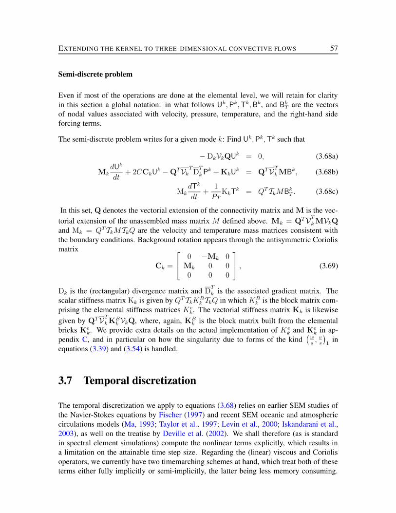
EXTENDING THE KERNEL TO THREE-DIMENSIONAL CONVECTIVE FLOWS 57
Semi-discrete problem
Even if most of the operations are done at the elemental level, we will retain for clarityin this section a global notation: in what follows Uk, Pk, Tk, Bk, and Bk
T are the vectorsof nodal values associated with velocity, pressure, temperature, and the right-hand sideforcing terms.
The semi-discrete problem writes for a given mode k: Find Uk, Pk, Tk such that
− DkVkQUk = 0, (3.68a)
MkdUk
dt+ 2CCkU
k − QTVkTD
T
k Pk + KkUk = QTVT
k MBk, (3.68b)
MkdTk
dt+
1
PrKkT
k = QTTkMBkT . (3.68c)
In this set, Q denotes the vectorial extension of the connectivity matrix and M is the vec-torial extension of the unassembled mass matrix M defined above. Mk = QTVT
k MVkQ
and Mk = QTTkMTkQ are the velocity and temperature mass matrices consistent withthe boundary conditions. Background rotation appears through the antisymmetric Coriolismatrix
Ck =
0 −Mk 0Mk 0 00 0 0
, (3.69)
Dk is the (rectangular) divergence matrix and DT
k is the associated gradient matrix. Thescalar stiffness matrix Kk is given by QTTkK
Bk TkQ in which KB
k is the block matrix com-prising the elemental stiffness matrices Ke
k. The vectorial stiffness matrix Kk is likewisegiven by QTVT
k KBk VkQ, where, again, KB
k is the block matrix built from the elementalbricks Ke
k. We provide extra details on the actual implementation of K ek and Ke
k in ap-pendix C, and in particular on how the singularity due to forms of the kind
(
ws, v
s
)
1in
equations (3.39) and (3.54) is handled.
3.7 Temporal discretization
The temporal discretization we apply to equations (3.68) relies on earlier SEM studies ofthe Navier-Stokes equations by Fischer (1997) and recent SEM oceanic and atmosphericcirculations models (Ma, 1993; Taylor et al., 1997; Levin et al., 2000; Iskandarani et al.,2003), as well on the treatise by Deville et al. (2002). We shall therefore (as is standardin spectral element simulations) compute the nonlinear terms explicitly, which results ina limitation on the attainable time step size. Regarding the (linear) viscous and Coriolisoperators, we currently have two timemarching schemes at hand, which treat both of theseterms either fully implicitly or semi-implicitly, the latter being less memory consuming.

EXTENDING THE KERNEL TO THREE-DIMENSIONAL CONVECTIVE FLOWS 58
The fully implicit case is necessary when stability is at stake. It is particularly relevantto the rapidly rotating limit when one is interested in studying the long-term behaviourof rotating fluids and needs to control efficiently inertial oscillations (Greenspan, 1990;Hollerbach, 2003).
In our approach, the temperature solve is decoupled from the velocity-pressure solve. Thecoupled velocity-pressure problem is handled following a consistent decoupling strategyapplied at the discrete level, resulting in an overal second-order temporal accuracy.
3.7.1 Timemarching
Let ∆t be the timestep and Ukn, Pk
n, Tkn, Bk
n, and BkTn denote the values of Uk, Pk, Tk, Bk,
and BkT at the discrete time tn = n∆t.
In the fully implicit case (hereafter referred to as FI), time derivatives are approximated by asecond-order backward differentiation formula of order 2 (BDF2), which is unconditionallystable. This gives
dUk, Tkdt
∣
∣
∣
∣
n+1
=3Uk
n+1, Tkn+1 − 4Uk
n, Tkn + Uk
n−1, Tkn−1
2∆t. (3.70)
In the semi-implicit case (hereafter referred to as SI), the use of a midpoint rule allows timederivatives to be approximated with a first order Euler formula
dUk, Tkdt
∣
∣
∣
∣
n+1
=Uk
n+1, Tkn+1 − Uk
n, Tkn
∆t, (3.71)
thus requiring less storage.
Nonlinear right-hand side forcing terms are approximated in both schemes by means of athird-order Adams-Bashforth formula (AB3), which, contrary to the AB2 formula, has astability region which has a non-zero intersection with the imaginary axis (Deville et al.,2002):
Bkn+1, B
kTn+1 =
23
12Bk
n, BkTn −
4
3Bk
n−1, BkTn−1 +
5
12Bk
n−2, BkTn−2. (3.72)
In practice, Bk and BkT contain quadratic terms which couple Fourier modes. They are
computed in the physical domain and then transformed back into Fourier space by meansof a fast Fourier transform algorithm (Frigo & Johnson, 1997). As we perform the domaindecomposition in the meridional plane, this procedure is local and does not require inter-processors communications. The explicit AB3 formula causes the timestep to be limited toa value proportional to the minimum grid spacing h:
∆t < Ch/U, (3.73)

EXTENDING THE KERNEL TO THREE-DIMENSIONAL CONVECTIVE FLOWS 59
in which C is an order 1 constant and U is the maximal pointwise velocity. For anaxisymmetric problem, h is equal to hmed, the minimal grid-spacing in the meridionalplane. The clustering of the GLL and WGLL points near elemental boundaries is such thathmed ∝ 1/ (neN
2). For a three-dimensional problem, using the equidistant Fourier gridin the azimuthal direction, we have observed that h is typically equal to a fraction of hmed,due to the clustering of points near Γ. We will address issues related to the so-called poleproblem in the discussion (§3.9).
As stated above, the linear viscous and Coriolis operators in equations (3.68b) and (3.68c)are treated either implicitly or semi-implicitly. In the latter case, they are approximatedusing a second-order Crank-Nicolson formula (also known as the trapezoidal rule):
Kk,CkUk∣
∣
n+1=
1
2
(
Kk,CkUkn+1 + Kk,CkUk
n
)
. (3.74)
KkTk∣
∣
n+1=
1
2
(
KkTkn+1 + KkT
kn
)
(3.75)
Finally, the pressure field Pkn+1 is written as
Pkn+1 = Pk
n + δPk, (3.76)
where δPk is the pressure increment to be computed.
After applying these different formulas, one ends up in both cases with the following prob-lem to solve at each time step
AkUkn+1 − QTVT
k DT
k δPk = Fkn+1, (3.77)
−DkVkQUkn+1 = 0, (3.78)
AkTkn+1 = Fk
Tn+1, (3.79)
in which Ak is a modified vectorial Helmholtz operator
Ak = ai∆t−1Mk + 2acCCk + avKk, (3.80)
in which (ai, ac, av) = (3/2, 1, 1)(FI) or (ai, ac, av) = (1, 1/2, 1/2)(SI). The right handside forcing term writes
Fkn+1 = QTVT
k (MBkn+1 + D
T
k Pkn) +
Mk∆t−1(2Ukn − 1
2Uk
n−1) (FI)
Mk∆t−1Ukn − CCkU
kn − 1
2KkU
kn (SI)
. (3.81)
The symmetric scalar Helmholtz operator Ak has the form
Ak = ai∆t−1Mk + avPr−1Kk, (3.82)
and the right hand side forcing term FkTn+1 writes
FkTn+1 = QTTkMBk
Tn+1 +
Mk∆t−1(2Tkn − 1
2Tk
n−1) (FI)
Mk∆t−1Tkn − 1
2KkT
kn (SI)
. (3.83)

EXTENDING THE KERNEL TO THREE-DIMENSIONAL CONVECTIVE FLOWS 60
3.7.2 Temperature solve
To obtain the value of the temperature at the next time step, we solve the equation AkTkn+1 =
FkTn+1 by means of a diagonally preconditioned conjugate gradient (PCG) method. The
value of ∆t imposed by the stability requirements (3.73) resulting from the AB3 formulais indeed typically such that Ak is diagonally dominant. As the quantities involved arecomplex numbers (except for T0 which is real), the real and imaginary parts of Tk
n+1 arecomputed independently. This remark applies to the velocity and pressure solves intro-duced below.
3.7.3 A discrete decoupling scheme for the velocity-pressuresubproblem
Turning now our attention to the modified Stokes problem involving velocity and pressure,we note that its four-dimensional character precludes a direct solve and we follow insteadthe decoupling strategy exposed by Fischer (1997), which was based upon earlier studiesby Maday et al.(1993) and Couzy (1995).
First of all, the so-called inhomogeneity gk is computed, according to
gk = −DkVkQA−1k Fk
n+1 = −DkVkQUk?, (3.84)
where Uk? can be interpreted as a first guess for the k-th velocity mode, which does notsatisfy the divergence-free constraint. The operator Ak is inverted iteratively, using a pre-conditioned stabilized biconjugate gradient method (van der Vorst, 1992) when C 6= 0, anda PCG algorithm otherwise. The preconditioner used is the diagonal of Ak, for the reasonsstated above.
The estimate Uk? is then improved through the calculation of the pressure increment δPk,which is obtained after inversion of the pseudo-Laplacian operator Ek:
δPk = E−1k gk, (3.85)
where Ek = a−1i ∆tDkVkQM−1
k QTVT
k DT
k . This symmetric operator is inverted by meansof a PCG algorithm. The preconditioner we use is an adaptation of the overlapping Schwarztechnique presented by Fischer (1997) to our cylindrical meridional problems. This refinedtechnique is unavoidable because of the poor conditioning of the pseudo-Laplacian opera-tor, which is defined accross the spaces Xk
h and Yh. We developed this technique at firstin the axisymmetric context (Fournier et al., 2003a), for which we typically found a factorof ten reduction in the iteration count in the pressure increment solve with respect to thenon-preconditoned case, resulting in a threefold decrease in the CPU time cost of the pres-sure calculation. We observe the same behaviour with the extension of the preconditionerto non-axisymmetric Fourier modes.
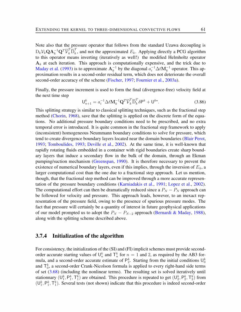
EXTENDING THE KERNEL TO THREE-DIMENSIONAL CONVECTIVE FLOWS 61
Note also that the pressure operator that follows from the standard Uzawa decoupling isDkVkQA−1
k QTVT
k DT
k , and not the approximated Ek. Applying directly a PCG algorithmto this operator means inverting (iteratively as well!) the modified Helmholtz operatorAk at each iteration. This approach is computationally expensive, and the trick due toMaday et al. (1993) is to approximate A−1
k by the diagonal a−1i ∆tM−1
k operator. This ap-proximation results in a second-order residual term, which does not deteriorate the overallsecond-order accuracy of the scheme (Fischer, 1997; Fournier et al., 2003a).
Finally, the pressure increment is used to form the final (divergence-free) velocity field atthe next time step
Ukn+1 = a−1
i ∆tM−1k QTVT
k DT
k δPk + Uk?. (3.86)
This splitting strategy is similar to classical splitting techniques, such as the fractional stepmethod (Chorin, 1968), save that the splitting is applied on the discrete form of the equa-tions. No additional pressure boundary conditions need to be prescribed, and no extratemporal error is introduced. It is quite common in the fractional step framework to apply(inconsistent) homogeneous Neummann boundary conditions to solve for pressure, whichtend to create divergence boundary layers located near the domain boundaries (Blair Perot,1993; Tomboulides, 1993; Deville et al., 2002). At the same time, it is well-known thatrapidly rotating fluids embedded in a container with rigid boundaries create sharp bound-ary layers that induce a secondary flow in the bulk of the domain, through an Ekmanpumping/suction mechanism (Greenspan, 1990). It is therefore necessary to prevent theexistence of numerical boundary layers, even if this implies, through the inversion of Ek, alarger computational cost than the one due to a fractional step approach. Let us mention,though, that the fractional step method can be improved through a more accurate represen-tation of the pressure boundary conditions (Karniadakis et al., 1991; Lopez et al., 2002).The computational effort can then be dramatically reduced since a PN − PN approach canbe followed for velocity and pressure. This approach leads, however, to an inexact rep-resentation of the pressure field, owing to the presence of spurious pressure modes. Thefact that pressure will certainly be a quantity of interest in future geophysical applicationsof our model prompted us to adopt the PN − PN−2 approach (Bernardi & Maday, 1988),along with the splitting scheme described above.
3.7.4 Initialization of the algorithm
For consistency, the initialization of the (SI) and (FI) implicit schemes must provide second-order accurate starting values of Uk
n and Tkn for n = 1 and 2, as required by the AB3 for-
mula, and a second-order accurate estimate of Pk2 . Starting from the initial conditions Uk
0
and Tk0 , a second-order Crank-Nicolson formula is applied to every right-hand side terms
of set (3.68) (including the nonlinear terms). The resulting set is solved iteratively untilstationnary (Uk
1, Pk1, T
k1) are obtained. This procedure is repeated to get (Uk
2, Pk2, T
k2) from
(Uk1, P
k1, T
k1). Several tests (not shown) indicate that this procedure is indeed second-order

EXTENDING THE KERNEL TO THREE-DIMENSIONAL CONVECTIVE FLOWS 62
accurate.
In the next section, the SI scheme will be used to study simple flows in a (non-rotating)vertical circular cylinder (§3.8.2), whereas we will turn to the FI scheme to compute thesolution to a Rayleigh-Bénard problem in a rapidly rotating spherical shell (§3.8.3).
3.8 Examples
We now validate our implementation of the Fourier-spectral element method through threedistinct problems. The first one (§3.8.1) is a Stokes problem in a spherical shell geometry,the analytical solution of which is known. It ignores any thermal effect and aims primarilyat checking the correctness of the spatial component of the model. Next (§3.8.2), we switchfrom a spherical shell to a vertical cylinder and study simple Rayleigh-Bénard problems fordifferent sets of boundary conditions, using the SI time scheme. Finally (§3.8.3), we returnto a spherical shell geometry and compute a Rayleigh-Bénard flow in a rapidly rotatingcontext (C = 103), for which reference published numerical solutions exist (Christensenet al., 2001). This last example is computed with the FI scheme.
3.8.1 Analytical Stokes flow in a spherical shell
In this section, an analytical Stokes flow is considered in order to check that the PN −PN−2 approach is properly implemented, and especially that the discrete velocity is indeeddivergence-free. The exercise presented here is a generalization of the axisymmetric studyshown in Fournier et al. (2003a). A nice property of this linear problem is that it allows toisolate different Fourier modes, thereby permitting the verification of the implementationof the essential axial conditions (3.41) independently.
The three-dimensional domain Ω is here a spherical shell of inner radius ri and outer radiusro (the radius ratio ri/ro being 1/3).
The Stokes problem of interest writes
∇2u −∇P + br = 0 in Ω, (3.87a)∇ · u = 0 in Ω, (3.87b)
u = 0 on ∂ Ω. (3.87c)
Note that r is the unit vector in the radial direction and that the prescribed forcing br we seekin equation (3.87a) is purely radial (it could be interpreted as an imposed buoyancy force).To define the analytical reference solution ua, we start by making the standard poloidal-toroidal decomposition of the velocity (see e.g. Dahlen & Tromp, 1998, appendix B):
ua = ∇× (Er) + ∇×∇× (F r), (3.88)

EXTENDING THE KERNEL TO THREE-DIMENSIONAL CONVECTIVE FLOWS 63
-/. 0
1324
5687956 7 :<;>=
5687?
1A@4
56CB9 D 56 B: 56CB?
1 44
56FE9 D 56FE: 56FE?
-/. GHG
1I2@@
5687956 7 :<;>=
5687?
1J@@@
56CB9 D 56 B: 56CB?
1 4@@
56FE9 D 56FE: 56FE?
Figure 3.6: Reference velocity fields for analytical Stokes benchmark of the Fourier-spectral element method in a spherical shell. Each case corresponds to a different sphericalharmonic (Ym
l ) structure. Left panel: l = 2 reference solutions, with angular order varyingfrom 0 to 2 (top to bottom). Right panel: l = 11 reference solutions, with angular ordervarying also from 0 to 2 (top to bottom). Isolines for the three cylindrical components areshown in the upper part of the meridional domain only. Solid (dashed) lines indicate pos-itive (negative) values. The (arbitrary) scale varies from harmonic to harmonic, but is thesame for the three components of the velocity of a given Ym
l .
where E and F are the toroidal and poloidal fields, respectively. Using this expansion, weautomatically satisfy equation (3.87b) with our reference velocity solution. Each field isthen sought in terms of spherical harmonics:
E,F, b, P(r, θ, φ) =∞∑
l=0
m=l∑
m=−l
Eml , Fm
l , bml , Pm
l (r)Yml (θ, φ), (3.89)
in which Yml is the spherical harmonic of degree l and order m. As the problem of interest
is linear, we can consider one harmonic at a time. The radial components of the first andsecond curls of equation (3.87a) are
Eml = 0, (3.90)
[
d2
dr2− l(l + 1)
r2
]2
Fml = bm
l . (3.91)

EXTENDING THE KERNEL TO THREE-DIMENSIONAL CONVECTIVE FLOWS 64
In the present case of a purely radial forcing, equation (3.90) tells us that the toroidal field isidentically zero. As far as the poloidal field is concerned, since equation (3.91) is a fourth-order equation, we need four boundary conditions, two each at ri and ro. The no-slipboundary conditions imply that:
Fml =
d
drFm
l = 0 at r = ri, ro. (3.92)
Once a couple (l,m) has been picked, the procedure for the test can be summarized asfollows:
1. Choose an expression for F ml that matches the boundary conditions (3.92).
2. Solve equation (3.91) analytically for the appropriate forcing bml .
3. Use this forcing as an input.
4. Solve the Stokes problem in the Fourier-spectral element framework, by applying anUzawa algorithm (Arrow et al., 1958).
5. Quantify the accuracy of the numerical solution uh with respect to the analyticalsolution ua.
The cases considered are shown on figure 3.6. We pick two spherical harmonic degrees, l =2 and l = 11. The former corresponds to a smooth velocity field varying slowly in space,while the latter gives rise to a field which varies on smaller length scales. In each case,we limited the study to the first three angular orders (m = 0, 1, 2), which correspond tothe three different sets of axial conditions (3.41). As shown on figure 3.6, these conditionsare met by construction when employing a basis of spherical harmonics. Moreover, thedifferent components of the velocity satisfy the following symmetry properties
us(s,−z) = (−1)l−mus(s, z), (3.93)uφ(s,−z) = (−1)l−muφ(s, z), (3.94)uz(s,−z) = (−1)l−m+1uz(s, z), (3.95)
and, consequently, analytical solutions are displayed in the upper part of the meridionaldomain only. The analytical solutions we define are also such that the s and z componentsus and uz are real, while the φ component uφ is imaginary. We therefore plot iuφ onfigure 3.6. One can notice for instance that the condition us + iuφ is satisfied on the axis Γin the cases (labelled Y1
2 and Y111) for which m = 1.
Results are shown in figures 3.7 (for l = 2) and 3.8 (for l = 11). They were computedvarying the polynomial order N and for a hierarchy of meshes of 1, 4, 16, and 64 ele-ments, obtained after successive refinements in the r and θ directions, as shown on fig-ures 3.7 and 3.8.

EXTENDING THE KERNEL TO THREE-DIMENSIONAL CONVECTIVE FLOWS 65
2 4 6 8 10 12 14 16 18 201.0e-09
1.0e-08
1.0e-07
1.0e-06
1.0e-05
1.0e-04
1.0e-03
1.0e-02
1.0e-01
1.0e+00
K
LNMPORQL M OTSL M OUQWVLNMPOXVYS
Z\[]
2 4 6 8 10 12 14 16 18 201.0e-09
1.0e-08
1.0e-07
1.0e-06
1.0e-05
1.0e-04
1.0e-03
1.0e-02
1.0e-01
1.0e+00
^
_N`acb_N`aed_N`afbWg_N`ahgYd
ikjl
2 4 6 8 10 12 14 16 18 201.0e-09
1.0e-08
1.0e-07
1.0e-06
1.0e-05
1.0e-04
1.0e-03
1.0e-02
1.0e-01
1.0e+00
m
nNopRqnNopTrnNopUqWsn o pXsYr
tvuu
Figure 3.7: L21 norm of error versus polynomial order for analytical Stokes benchmark of
the Fourier-spectral element method (FSEM) in a spherical shell for spherical harmonicdegree 2, and angular order 0, 1, and 2 (left to right). Solutions were computed in each casewith four different meridional spectral element grids, comprising 1, 4, 16 and 64 elements.
2 4 6 8 10 12 14 16 18 20 22 241.0e-09
1.0e-08
1.0e-07
1.0e-06
1.0e-05
1.0e-04
1.0e-03
1.0e-02
1.0e-01
1.0e+00
1.0e+01
w
x\yzz
2 4 6 8 10 12 14 16 18 20 22 241.0e-09
1.0e-08
1.0e-07
1.0e-06
1.0e-05
1.0e-04
1.0e-03
1.0e-02
1.0e-01
1.0e+00
1.0e+01
|
k~~~
2 4 6 8 10 12 14 16 18 20 22 241.0e-09
1.0e-08
1.0e-07
1.0e-06
1.0e-05
1.0e-04
1.0e-03
1.0e-02
1.0e-01
1.0e+00
1.0e+01
v
Figure 3.8: L21 norm of error versus polynomial order for analytical Stokes benchmark of
the FSEM in a spherical shell for spherical harmonic degree 11 and angular order 0, 1, and2 (left to right).

EXTENDING THE KERNEL TO THREE-DIMENSIONAL CONVECTIVE FLOWS 66
In each case, the relative error e decreases exponentially when the polynomial order isincreased. The error also decreases (algebraically) at constant N when the number ofelements ne is increased. At constant ne, the geometric rate of convergence (correspondingto e ∝ exp(−aN), where a is a constant) is reached very soon in the smooth situation(l = 2), even when a single spectral element is used, as illustrated in figure 3.7. It is harderto obtain this behaviour in the small scale situation (figure 3.8), and a larger ne is requiredto enter the domain of geometric convergence for moderate values of N .
Let us stress that in order to obtain these results, it is necessary to use an analytical expres-sion for the mapping from the parent element to the deformed elements. A subparametricmapping does not approximate properly a spherical interface and induces for instance arelative residual error of 10−5 when ne = 16 (not shown).
These results show the correctness of the implementation of the PN − PN−2 method in theFourier-spectral element context, and in particular the proper enforcement of the axial con-ditions (3.41). We can also use this simple example to define the following rule-of-thumb:In a smooth situation (l = 2 here), using a uniform mesh, the following combinations of(ne, N) give the same (satisfactory) level of accuracy
(1, 16) ∼ (4, 12) ∼ (16, 9) ∼ (64, 7). (3.96)
3.8.2 Rayleigh-Bénard convection in a vertical circular cylinder
We now switch from a spherical shell to a vertical circular cylinder and consider the prob-lem of thermal convection in such a cylinder heated from below. This idealized system hasbeen considered to study the onset of convective instabilities, convection beyond its onset,secondary instabilites, and pattern formations (Rosenblat, 1982; Neumann, 1990; Touihriet al., 1999; Hof et al., 1999). Aside from their theoretical interest, these studies are alsomotivated by the interest in the control of crystal growth and the heat and mass transferresulting from convective motion in the melt (see Neumann, 1990, and references therein).
Our goal in this section is simply to reproduce some of the results obtained by Neumann(1990) in order to validate the FSEM in an other (well-known) geometry and for differentboundary conditions.
Geometry is controlled by the aspect ratio of the cylinder
a =h
d, (3.97)
in which h is the height of the cylinder (−1/2h ≤ z ≤ 1/2h) and d its diameter (seefigure 3.9, right). A temperature difference ∆T is imposed between the bottom and the topof the cylinder, in a uniform gravity field g. The choice of scales of Neumann (1990) isslightly different from the one made in equations (3.4). Lengths are scaled with h, velocity

EXTENDING THE KERNEL TO THREE-DIMENSIONAL CONVECTIVE FLOWS 67
with κ/h, pressure with ρκ2/h, time with h2/κ, and temperature with ∆T . Neumann’sBoussinesq equations then write
∇ · u = 0, (3.98a)∂tu + u · ∇u = −∇P + Pr∇2u + RPrT z, (3.98b)∂tT + u · ∇T = ∇2T − u · ∇Ts. (3.98c)
The expression for the Rayleigh number R is in this case
R =gαh3∆T
νκ, (3.99)
which is the classical formula for this number (see Chandrasekhar, 1961, chap. 1). Thestatic temperature and pressure profiles are given by Ts(z) = 1/2 − z and p0 = const. +RPr(z−z2)/2. We shall consider two sets of boundary conditions. The first set has stress-free, isothermal top and bottom boundaries, and an adiabatic sidewall for which stress-freeboundary conditions are also applied:
∂zus = ∂zuφ = uz = T = 0 on z = ±1/2, 0 ≤ s < d/2,us = ∂s(suφ) = ∂suz = ∂sT = 0 on s = d/2, −1/2 < z < 1/2.
(3.100)This case corresponds to the so-called shear-free cylinder case in Neumann (1990). Thesecond set of boundary conditions has no-slip kinematic boundary conditions, and the samethermal boundary conditions:
us = uφ = uz = T = 0 on z = ±1/2, 0 ≤ s < d/2,us = uφ = uz = ∂sT = 0 on s = d/2, −1/2 < z < 1/2.
(3.101)
This is the rigid cylinder case. Switching from the shear-free case to the rigid case isaccomplished in our approach through the appropriate modifications of the velocity maskarrays Vk introduced in section 3.6.2.
To solve these equations, Neumann (1990) employed a finite difference method on a three-dimensional, cylindrical, staggered grid, in an approach similar to the one proposed earlierby Williams (1969). We retain two of the cases he considered. The first deals with thelinear growth rate σ of the convective instability occuring in a shear-free cylinder of aspectratio a = 0.2899, for Pr = 1 and R = 1000. Rosenblat (1982) showed analytically thatthe critical value of the Rayleigh number Rc for these geometry and boundary conditionsis 657.51, corresponding to an axisymmetric instability. The expression of the associatedgrowth rate is (Neumann, 1990)
σ = −1
2
(
n2π2 + λ2j
)
(1 + Pr)
1 ±[
1 − 4Pr(1 − R/Rc)
(1 + Pr)2
]1
2
, (3.102)
where n refers to the number of zeros of the solution in the vertical direction, called thevertical wavenumber, and j is the radial wavenumber: λj is the jth positive root determined

EXTENDING THE KERNEL TO THREE-DIMENSIONAL CONVECTIVE FLOWS 68
3
hHH¡
¢¤£¦¥§
¢¤£¦¥
¢¤£ ¥©¨
¢¤£ ¥©ª
¢¤£ ¥¬« ¢¤£ ¥§¢¤£ ¥ ¢W£ ¥©¨
® ¯°
±²´³¶µ·
±U²c¸ ³¶µ·
® ¯¹º »
¼
½¿¾ÁÀ
Figure 3.9: Left: Difference between the numerical (σh) and analytical (σa) valuesof growth exponent of axisymmetric convective instability in a shear free cylinder fora = 0.2899, an adiabatic sidewall, R=1000 and Pr = 1, as a function of the numeri-cal timestep ∆t. The spectral element mesh consists of four spectral elements of varyingpolynomial order; squares: N = 6; diamonds: N = 8. For reference, two curves areshown, illustrating first and second order behaviours with dashed and dotted line, respec-tively. Right: N = 8 mesh. The height of the cylinder is h and its diameter is d.
by the condition J1(λ/2a) = 0, J1 being the Bessel function of order 1. For R = 1000 andPr = 1, we find σa = 3.4532.
In order to try and retrieve this value numerically, we get rid of the nonlinear interactions inthe Boussinesq equations (3.98), and timestep the resulting coupled linear set, starting withan initial random, axisymmetric temperature distribution. We do so using the semi-implicitscheme described previously in section 3.7. The convective instability eventually sets inand grows. Due to the absence of nonlinearities, we have to stop its runaway growth whenthe energy of the fluid Ek exceeds some threshold. We then determine σ by fitting Ek(t)with an exponential.
Results are displayed on figure 3.9, left, where the difference between the numerical growthrate σh and σa is plotted against the timestep. They were obtained using a meridional meshcomprising ne = 4 spectral elements of varying polynomial order (N = 6 and 8) - figure3.9 shows the N = 8 mesh. The structure of the convective instability being spatiallysimple enough (not shown here, see Neumann, 1990, figure 4), using N = 6 (squares)proves to be sufficient to properly resolve the instability and get the expected growth rate.This is confirmed by the N = 8 (diamonds) results. More interestingly, the dotted curveon figure 3.9, left, indicates that the dependence of the difference on the timestep size is ofsecond order, confirming the second-order accuracy of the semi-implicit timescheme.
Next, we consider a rigid cylinder of aspect ratio a = 1, filled with water (Pr = 6.7).

EXTENDING THE KERNEL TO THREE-DIMENSIONAL CONVECTIVE FLOWS 69
R = 17, 500
 ÂÄÃ
Å
Å Ã Â\Æ ÂÇÃ Å Æ Å Ã
R = 50, 000
È ÈÄÉ
Ê
Ê É È\Ë ÈÇÉ Ê Ë Ê É
Figure 3.10: Left: isocontours of normalized horizontal velocity in the horizontal midplane(z = 0) for a = 1, Pr = 6.7, R = 17, 500 (top) and R = 50, 000 (bottom), in the rigidcylinder case. Contour every 0.1, solid lines mean positive values, and dashed lines indicatenegative values. This (steady) circulation is not axisymmetric and has predominantly ak = 1 Fourier character. The vertical planes of symmetry are denoted with (AA’) and(BB’). Right: vertical cross-sections along these symmetry planes. The scale used forvelocity vectors along (AA’) is larger than scale used along (BB’) by a factor 2.5.

EXTENDING THE KERNEL TO THREE-DIMENSIONAL CONVECTIVE FLOWS 70
We prescribe two different Rayleigh numbers, R = 17, 500 and R = 50, 000, as in Neu-mann (1990). With this aspect ratio and these R’s, Neumann (1990) found only one non-axisymmetric stable steady solution, independent of the initial conditions, correspondingto the k = 1 Fourier mode. Using the Fourier-spectral element approach, we were ableto retrieve his findings; our results appear on figure 3.10. The horizontal slices showingthe vertical velocity profiles (figure 3.10, left) highlight a simple circulation: hot fluid isascending on one side of the cylinder and cold fluid is sinking on the other side. As theRayleigh number is increased the inclination of this roll is more pronunced, as shown bythe two (AA’) vertical slices of figure 3.10. A secondary circulation consisting of fourrolls is sumperimposed on this basic flow. It is of smaller magnitude (the scale used forthe (BB’) slices is 2.5 smaller than the one used for the (AA’) slices) and has also beenobserved in experiments (Müller et al., 1984). The results shown on figure 3.10 are in verygood (qualitative) agreement with those of Neumann (1990), figures 7 and 8.
To conclude this paragraph, let us stress that Rayleigh-Bénard convection in a (rigid orshear-free) cylinder can certainly generate fluid flows substantially more complicated thanthe simple cases we considered in this section. Their (fascinating) study is beyond thescope of this paper, in which we simply intend to show the versatily of the FSEM in termsof geometry and boundary conditions.
3.8.3 Thermal convection in a rotating spherical shell
Over the past decade, much has been learned on dynamo action through the numerical sim-ulations of convection-driven magnetohydrodynamic dynamos in rotating spherical shells;see Busse (2000); Dormy et al. (2000); Kono & Roberts (2002); Glatzmaier (2002) for re-cent reviews. Recently, in an attempt to increase the confidence in existing codes and toprovide a well-established standard solution for codes being developed, Christensen et al.(2001) proposed a numerical dynamo benchmark calculation.
The first case of this benchmark is purely hydrodynamic (no magnetic effect at all) andprovides an interesting and challenging test for our code. In a spherical shell Ω of innerradius ri and outer radius ro, temperature is fixed to To and To + ∆T on the outer and innerboundaries, respectively. The equations are scaled with D = ro − ri as the fundamentallength scale, which makes the dimensionsless radii equal to ro = 20/13 and ri = 7/13.The choice of scales is the same as the one exposed in section 3.2 and leads to the followingset of dimensionless equations:
∇ · u = 0, (3.103a)
E(
∂tu + u · ∇u −∇2u)
+ 2z × u = −∇P + Rr
ro
T, (3.103b)
∂tT + u · ∇T =1
Pr∇2T − u · ∇Ts. (3.103c)

EXTENDING THE KERNEL TO THREE-DIMENSIONAL CONVECTIVE FLOWS 71
Non-dimensional control parameters are the (modified) Rayleigh number
R =αgo∆TD
νω, (3.104)
where α is the coefficient of thermal expansivity and go is gravity at the outer radius, theEkman number and the Prandtl number Pr, which we already defined in equation (3.9).The values used in the benchmarks are R = 100, E = 10−3 (or, equivalently, C = 103),and Pr = 1. The static, radial temperature profile Ts is given by
Ts(r) =rori
r− ri. (3.105)
Furthermore, no-slip boundary conditions are used and velocity must vanish on the rigidboundaries. Initial conditions consist of a zero velocity field and of a temperature pertur-bation of degree and order four:
T (r, θ, φ; t = 0) =21√
17920π(1 − 3x2 + 3x4 − x6) sin4 θ cos 4φ, (3.106)
where x = 2r − ri − ro.
We solve this problem with the FI scheme described in section 3.7. A quasi-stationarysolution is reached within approximately 1 time unit, and Christensen et al. express it by avector function of the form
(u, P, T ) = f(r, θ, φ − ωdt), (3.107)
in which ωd is the drift frequency.
The solution is symmetric about the equator and has fourfold symmetry in longitude. Fig-ure 3.11 shows two slices representing the temperature field (left) and the velocity andpressure fields (right) at the equator. The fourfold azimuthal symmetry is clear on theserepresentations and the spiralling aspect of temperature contours is a classical feature ofconvective patterns in a rapidly rotating fluid. On figure 3.11, right, pressure contours showthat pressure highs are associated with anticyclonic motions while low pressure regions areconnected with cyclonic motions, an ubiquitous observation in the Earth’s atmosphere. Fig-ure 3.12 shows a three-dimensional image of the solution. Two isosurfaces for temperatureare represented, corresponding to cold (blue) and hot (yellow) thermal anomalies. Somevelocity vectors are also plotted (color scale indicates magnitude of velocity) in order tooutline the three-dimensional circulation inside the shell. As the solution is symmetricabout the equator, results exposed in what follows correspond to FSEM calculations per-formed in the upper part of the shell only. Moreover, the fourfold symmetry in longitudeleads to a reduction of the cost of the calculation by a another factor of four, as modeswhich are only multiple of 4 are involved. Figure 3.13 shows an example of a mesh used tocompute the rotating Rayleigh-Bénard flow. It consists of 4 spectral elements of order 14coupled with K + 1 = 32 Fourier modes in longitude φ. For this problem, nonlinear terms
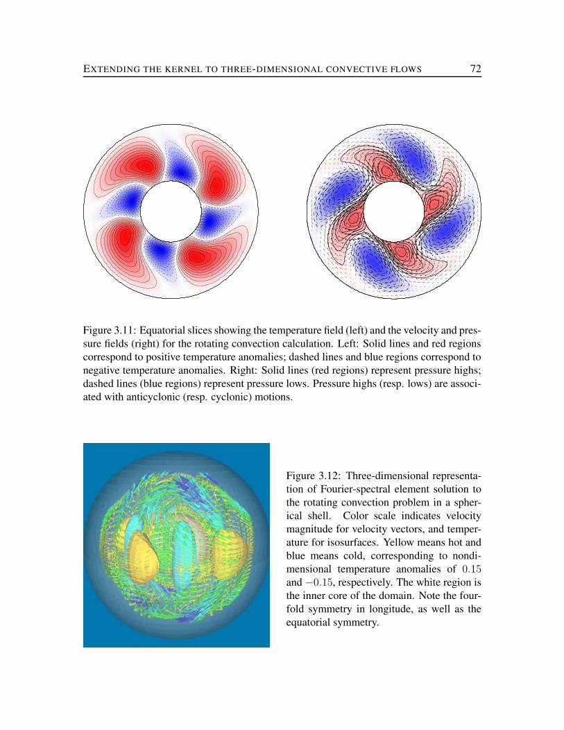
EXTENDING THE KERNEL TO THREE-DIMENSIONAL CONVECTIVE FLOWS 72
Figure 3.11: Equatorial slices showing the temperature field (left) and the velocity and pres-sure fields (right) for the rotating convection calculation. Left: Solid lines and red regionscorrespond to positive temperature anomalies; dashed lines and blue regions correspond tonegative temperature anomalies. Right: Solid lines (red regions) represent pressure highs;dashed lines (blue regions) represent pressure lows. Pressure highs (resp. lows) are associ-ated with anticyclonic (resp. cyclonic) motions.
Figure 3.12: Three-dimensional representa-tion of Fourier-spectral element solution tothe rotating convection problem in a spher-ical shell. Color scale indicates velocitymagnitude for velocity vectors, and temper-ature for isosurfaces. Yellow means hot andblue means cold, corresponding to nondi-mensional temperature anomalies of 0.15and −0.15, respectively. The white region isthe inner core of the domain. Note the four-fold symmetry in longitude, as well as theequatorial symmetry.

EXTENDING THE KERNEL TO THREE-DIMENSIONAL CONVECTIVE FLOWS 73
Figure 3.13: Example of a Fourier-spectral element mesh used to compute the rotatingRayleigh-Bénard flow. It consists of 4 spectral elements of order N = 14 in the (s, z)meridional plane coupled with K + 1 = 32 Fourier modes in longitude φ. Nonlinear termsin φ are computed pseudo-spectrally on a grid of 64 points in longitude.
Table 3.1: Contributors to case 0 of numerical dynamo benchmark, and their numericalmethod. Ym
l means that an expansion in spherical harmonics is used in the horizontaldirection. In radius, Chebyshev polynomials or finite differences (FD) are employed. In thislatter case, it is followed by the order of the method, and NE means that a non-equidistantradial grid spacing is possible, typically with a refinement toward the shell boundariesr = ri and r = ro to better resolve Ekman boundary layers. ST means that pressure isdefined on staggered grid points (it is not removed by taking the curl of the momentumequation).
Group Numerical MethodACD Aubert, Cardin, and Dormy. FD2_NE-Ym
l
CWG Christensen, Wicht, and Glatzmaier. Chebyshev-Yml
GJZ Gibbons, Jones, and Zhang. FD4_NE-Yml
TMH Takahashi, Matsushima, and Honkura. FD2_NE_ST-Yml

EXTENDING THE KERNEL TO THREE-DIMENSIONAL CONVECTIVE FLOWS 74
Table 3.2: Summary of results for case 0 of numerical dynamo benchmark. The last twolines indicate the standard solution to this problem, as defined in Christensen et al. (2001),along with the associated error limits. ne is the number of elements used in the meridionalplane, N is the polynomial order of the Legendre approximation, and K is the maximumwave number used in the φ direction. Due to the equatorial symmetry, calculations areperformed in the upper (northern) part of the shell only. The star indicates that results onthis row were obtained using the mesh shown on figure 3.13.
ne N K Resol. ekin ωd Ttot(x0) uφ(x0)1 14 31 19.3 58.2880 0.14676 0.42809 −10.15331 18 31 22.6 58.3518 0.18127 0.42813 −10.15801 22 31 25.7 58.3474 0.18235 0.42812 −10.15694* 14 31 30.0 58.3471 0.18230 0.42812 −10.15674 18 63 47.6 58.3472 0.18232 0.42811 −10.1570Standard solution: 58.348 0.1824 0.42812 −10.1571Uncertainties: 0.05 0.005 0.00012 0.002
are computed pseudo-spectrally on a grid of 2(K +1) points in longitude and no dealiasingprocedure, such as the 2/3 rule (Orszag, 1971), was necessary for this calculation.
Table 3.1 lists contributors to the benchmark and their numerical methods. All contributorsuse a spherical harmonic representation of the field variables in the horizonthal (θ, φ) plane,along with some form of discretization in the radial direction - finite differences (FD) orChebyshev polynomials. Each group follows an approach which is therefore similar to theone we use to define the analytical Stokes flow of section 3.8.1: a poloidal-toroidal decom-position of the velocity field is performed, and pressure is most of the time eliminated bytaking the curl of equation (3.103b). The resulting equations for the poloidal, toroidal andtemperature scalars are timestepped using standard schemes (typically Crank-Nicolson forviscous terms and Adams-Bashforth for nonlinear terms). For further details, see referencesin Christensen et al. (2001).
Contributors had to provide global averages as well as local data for the quasi-steady state.The former are the mean kinetic energy ekin and the value of the drift frequency ωd. Thelatter include the value of the total temperature Ttot (sum of the static temperature andthe temperature perturbation) and the azimuthal velocity uφ at a point x0 at mid-depth(r = (ri + ro)/2) in the equatorial plane (θ = π/2), the longitude of which is given by theconditions ur = 0 and ∂φur > 0. Christensen et al. (2001) used this definition to pick apoint whose position is fixed in the drifting frame of reference.
Results are plotted on figure 3.14, as a function of the spatial resolution, defined as thethird root of the number of degrees of freedom for each scalar variable. We used table 1of Christensen et al. (2001) to plot contributors’ results. We superimposed results obtained

EXTENDING THE KERNEL TO THREE-DIMENSIONAL CONVECTIVE FLOWS 75
15 20 25 30 35 40 45 50 55 60 65 70 75 8058.20
58.25
58.30
58.35
58.40
58.45
58.50
58.55
58.60
̶ÍYΤÏÐ ÑÒWÓ ÏÔ
ÕÖØ×ÚÙ
Û Ü Ý Þ
ßáàãâàPä¿ååçæ¦èéáêCëéìí îî ïð©ñò
15 20 25 30 35 40 45 50 55 60 65 70 75 800.140
0.145
0.150
0.155
0.160
0.165
0.170
0.175
0.180
0.185
0.190
0.195
0.200
ó¶ôYõ¤ö÷ øù¤ú öû
üý
þ ÿ
15 20 25 30 35 40 45 50 55 60 65 70 75 800.42700
0.42710
0.42720
0.42730
0.42740
0.42750
0.42760
0.42770
0.42780
0.42790
0.42800
0.42810
0.42820
0.42830
0.42840
! "$# % &
')(+*,(.-0/213
465 758:9 ;<=>?>A@CBBD0EFGIHFKJL MKM N OP+Q
15 20 25 30 35 40 45 50 55 60 65 70 75 80-10.170
-10.165
-10.160
-10.155
-10.150
-10.145
-10.140
-10.135
-10.130
RTSU V6W X$Y Z V6[
\)])^0_2`a
b cd+e fg
hijiAkmlln:opqIrpKs6t uKu vxwy+z
Figure 3.14: Convergence of results for rotating convection calculation. Results for ACD,CWG, GJZ, and TMH plotted after table 1 of Christensen et al. (2001). For details on themethods used by these groups, see table 3.1 and references in Christensen et al. (2001).Results obtained by the FSEM in blue, with right triangles. Global data on top row: meankinetic energy ekin (left) and drift frequency ωd (right). Local data on bottom row: totaltemperature Ttot (left) and azimuthal velocity uφ (right). Resolution is defined as the thirdroot of the number of degree of freedoms for each scalar variables.

EXTENDING THE KERNEL TO THREE-DIMENSIONAL CONVECTIVE FLOWS 76
via the FSEM. These are also listed in table 3.2, along with the suggested standard valuesof Christensen et al. (2001). Christensen et al. (2001) pointed out that the different resultsobtained by the contributors converge to the same values within better than 2%. The rate ofconvergence being fast in the spectral (Chebyshev) case, and slow when finite differencingis used in the radial direction. It appears that the number of grid points in the Ekmanboundary layers is critical to properly resolve the solution. The clustering of the Chebyshevpoints near the boundaries is clearly an advantage in this situation. Also, as pointed out byChristensen et al. (2001), this case is simple “in the sense that the spatial spectra drop offrapidly with wavenumber and time dependence is weak, which makes it ideally suited forspectral methods”.
As a matter of fact, table 3.2 shows that the results obtained here are in excellent agreementwith the suggested values (to within better than 0.05% in all cases). As seen on figure 3.14,the rate of convergence is also very satisfactory, and the FSEM is in this respect equivalentto the Chebyshev-Ym
l approach. The smooth character of the sought solution promptedus to obtain finer resolutions by increasing the polynomial order N to large values andby keeping the total number of elements ne very small. We benefited therefore from theclustering of the GLL points near the boundaries and the associated good resolution of theEkman boundary layers. In more chaotic, time-dependent situations, timestepping issuescould however lead us to keep the polynomial order low (typically between 6 and 12) andto increase ne to obtain finer resolutions.
3.9 Discussion - Conclusion
We have presented a Fourier-spectral element model of thermal convection for a fluid fill-ing an axisymmetric container, in a rapidly rotating reference frame. This model, whichrelies heavily on the recent theoretical work of Bernardi et al. (1999), is based upon aFourier expansion of the field variables in the periodic direction, and the resolution ofthe associated meridional problems via the spectral element method. A weighted Gauss-Lobatto-Legendre quadrature has been introduced to treat those elements sharing an edgewith the axis of symmetry of the three-dimensional domain. Inside a meridional element,velocity and temperature are approximated by polynomials of order N in each directionof space, and a slightly lower order (N − 2) is used to discretize pressure. The resultingsemi-discrete system is timestepped using second-order schemes: the Coriolis and viscousforces are discretized either semi-implicitly or fully-implicitly. Nonlinear terms are in bothcases approximated by an explicit third-order Adams-Bashforth formula.
Three examples have illustrated the accuracy of this approach. The steady Stokes problemin a spherical shell (§3.8.1) proved the validity of our implementation of the meridionalbricks of the method (mass matrix, divergence matrix, stiffness matrix, mask arrays), andit highlighted its spectral convergence properties. Not surprisingly, to achieve acceptableaccuracy, it is much more efficient to increase N , keeping the number of elements ne con-

EXTENDING THE KERNEL TO THREE-DIMENSIONAL CONVECTIVE FLOWS 77
stant, rather than to increase ne at constant N – this is precisely the difference between theexponential convergence of spectral methods and the algebraic convergence of finite differ-ence and finite element methods. We considered next (§3.8.2) standard Rayleigh-Bénardconvection in a cylinder heated from below and found good agreement between our cal-culations and the analytical results of Rosenblat (1982) and the finite difference model ofNeumann (1990), varying the aspect ratio of the cylinder and the velocity boundary con-ditions. Finally (§3.8.3), we studied the rotating Rayleigh-Bénard benchmark case in aspherical shell of Christensen et al. (2001). This problem combined all the ingredients ofthe governing equations (3.5) and the smoothness of the sought solution prompted us to usea minimal ne and large N to reproduce the reference solution with an excellent agreement.
The previous enthusiastic remarks praising spectral vs. algebraic convergence have to beconfronted with practical considerations: when dealing with a nonlinear, unsteady problem(highly supercritical convection for instance), a high enough resolution is needed, whichhas a drastic influence on the timestep size ∆t. The explicit treatment of nonlinearitiesimplies indeed that ∆t can not exceed a value which is proportional to the smallest distanceh between two grid points. In our case, the clustering of the GLL and WGLL points near theelement boundaries is such that the meridional minimal grid spacing hmed is proportionalto 1/(neN
2). Figure 3.15 shows the minimal grid spacing hmed for the mesh of figure3.13 (consisting of four spectral elements) for different values of N , along with the overallh that results from the use of a Fourier grid of 64 equidistant points in longitude. Weobserve that in this case hmed ≈ 5.70h. This follows from the clustering of points in thepolar regions, which is the root of the so-called pole problem (Boyd, 2001, §18.10). Thismight not be so crucial for our purposes, since calculations at large C for which this modelis ultimately aimed require to resolve very thin Ekman boundary layers in the meridionalplane. For larger and larger Coriolis numbers, the increase in meridional resolution is likelyto outweigh the increase in K, and therefore hmed should be closer to h. In a stronglynonlinear context, one should anyhow use a constant (moderate) value of N (on the orderof 10) and refine the resolution by increasing ne, which allows for the model to be runon more processors. As far as performances are concerned, let us stress that the currentversion of the code has yet to be optimized (at the serial and parallel levels), following forinstance the precepts of Deville et al. (2002, chap. 8). This task has been recently initiated,now that the model is anchored on robust (accurate) foundations. In particular, we wish todevelop a new preconditioner for the modified Helmholtz operator (3.80) which, unlike thediagonal preconditioner, does not restrict the timestep to a fraction of C−1 (a fraction ofω−1 if one restores dimensions).
The FSEM has an overall complexity of O(KneN3), and a complexity per processor of
O(KneN3/np), if np denotes the number of processors. It is fundamental to obtain good
scaling performances and even more efficient solvers for this approach to allow to tacklechallenging problems in planetary dynamics. An already very positive news in this respectis that the FSEM does not require a lot of memory, thanks to the problem reduction inlongitude and the tensorized formulation, which preserves us from storing large matrices.In particular, switching from the semi-implicit to fully-implicit scheme has a minimal im-
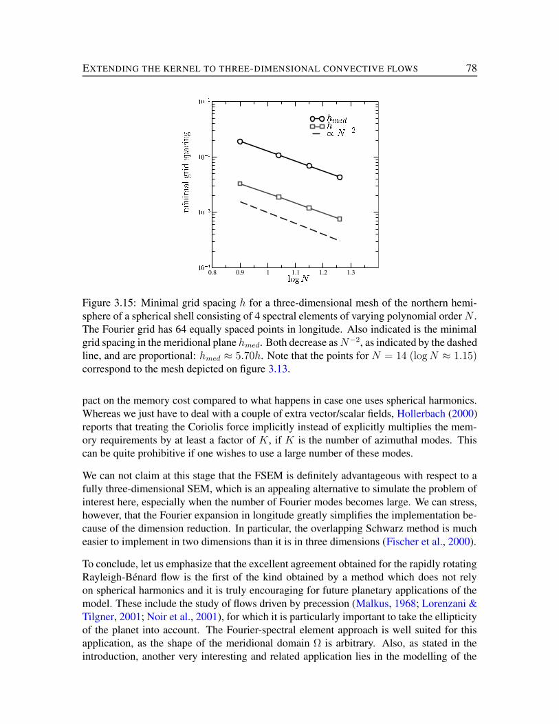
EXTENDING THE KERNEL TO THREE-DIMENSIONAL CONVECTIVE FLOWS 78
0.8 0.9 1 1.1 1.2 1.3
|~A
0,
0
:
:
Figure 3.15: Minimal grid spacing h for a three-dimensional mesh of the northern hemi-sphere of a spherical shell consisting of 4 spectral elements of varying polynomial order N .The Fourier grid has 64 equally spaced points in longitude. Also indicated is the minimalgrid spacing in the meridional plane hmed. Both decrease as N−2, as indicated by the dashedline, and are proportional: hmed ≈ 5.70h. Note that the points for N = 14 (log N ≈ 1.15)correspond to the mesh depicted on figure 3.13.
pact on the memory cost compared to what happens in case one uses spherical harmonics.Whereas we just have to deal with a couple of extra vector/scalar fields, Hollerbach (2000)reports that treating the Coriolis force implicitly instead of explicitly multiplies the mem-ory requirements by at least a factor of K, if K is the number of azimuthal modes. Thiscan be quite prohibitive if one wishes to use a large number of these modes.
We can not claim at this stage that the FSEM is definitely advantageous with respect to afully three-dimensional SEM, which is an appealing alternative to simulate the problem ofinterest here, especially when the number of Fourier modes becomes large. We can stress,however, that the Fourier expansion in longitude greatly simplifies the implementation be-cause of the dimension reduction. In particular, the overlapping Schwarz method is mucheasier to implement in two dimensions than it is in three dimensions (Fischer et al., 2000).
To conclude, let us emphasize that the excellent agreement obtained for the rapidly rotatingRayleigh-Bénard flow is the first of the kind obtained by a method which does not relyon spherical harmonics and it is truly encouraging for future planetary applications of themodel. These include the study of flows driven by precession (Malkus, 1968; Lorenzani &Tilgner, 2001; Noir et al., 2001), for which it is particularly important to take the ellipticityof the planet into account. The Fourier-spectral element approach is well suited for thisapplication, as the shape of the meridional domain Ω is arbitrary. Also, as stated in theintroduction, another very interesting and related application lies in the modelling of the

EXTENDING THE KERNEL TO THREE-DIMENSIONAL CONVECTIVE FLOWS 79
dynamo process at work for instance in the Earth’s outer core. The main difference be-tween the Navier-Stokes equation and the so-called induction equation which governs theevolution of the magnetic field lies in the boundary conditions. On the outer boundary ofthe region filled by the convecting metallic liquid, the magnetic field has to be connectedwith an exterior potential field. This connection is straightforward if one is using spheri-cal harmonics (Glatzmaier, 1984) but less amenable to a local method like ours. We arecurrently investigating this issue.
Chapter 4
Fluid flows driven by thermal convectionand precession
4.1 Introduction
Aside from its engineering applications related to the control of space vehicles (Vanyo &Likins, 1971), precession has also attracted the attention of geophysicists, since Malkus(1968) advocated it as a plausible source of energy for the geodynamo, the process at workin the Earth’s core, and responsible for the generation of its magnetic field.
Figure 4.1 illustrates the mechanism that controls the precession of the Earth: The instan-taneous axis of rotation of the Earth is inclined with respect to the normal to the eclipticplane, and the gravitational action of the Sun (and Moon) on the Earth’s equatorial bulgeexerts a torque that tends to pull the bulge into alignment with the instantaneous Earth-Sun(or Moon) axis. This torque causes the retrograde precession of the spin axis of the Earthabout the normal to the ecliptic plane, with a period of 25770 yr (Yoder, 1995).
Malkus (1968) conducted a series of experiments involving a spheroidal cavity filled withwater, and precessing at different precession rates. He first observed a steady solution, ofthe form of a solid-body rotation organized around an axis tilted with respect to the direc-tion of the ‘experimental’ daily rotation vector ωd (Malkus, 1968, figure 1.1). Increasingthe precession rate, the flow became unstable (Malkus, 1968, figures 1.2-1.3) and even-tually fully turbulent (Malkus, 1968, figure 1.4). Assuming that the turbulent regime wasappropriate for the core, Malkus derived an estimate of the energy that could be fed into thegeodynamo and reached a positive conclusion regarding the ability of precession to sustainthe dynamo. More precisely, he found the input coming from turbulent precession to beclose to 2.5 1010 W. With retrospect, this figure still appears quite small when comparedwith recent estimates of the needs of the geodynamo, which lie in the 1011 W − 2 1012 Wrange (Buffett, 2002; Roberts et al., 2003).
80

FLUID FLOWS DRIVEN BY THERMAL CONVECTION AND PRECESSION 81
Figure 4.1: Schematic representation of the precessing Earth. The angle β between thedaily rotation vector ωd and the normal to the ecliptic plane is 23.5 °. The precession of theEarth is retrograde, as indicated by the orientation of the precession vector ωp. The periodof precession is 2π/ωp = 25770 yr (Yoder, 1995).
Some years later, Rochester et al. (1975) rejected Malkus’ proposition, arguing that theprecession of the Earth had not net effect on the core, since the forcing it induces hasa diurnal periodicity in the reference frame rotating with the Earth. Contrary to Malkus’view, their argument was based on the assumption that the response of the core was laminar,thereby ignoring possible longer timescales that could arise from turbulent motions. Theyestimated the power originating from precession to be close to 108 W, a number which was,even at that time, far too small. We should also mention the work by Loper (1975), whoincluded electromagnetic effects in his –laminar– study, and found an input even smaller,of 3 107 W. Loper’s estimate was used for a long time to disregard precession as a plausiblesource of energy for the geodynamo.
More recently, Kerswell (1996) derived an upper bound of the energy that could be dis-sipated in turbulent precession. He found a dissipation rate fourteen orders of magnitudelarger than Loper’s value! Of course, this upper bound is unlikely to be achieved in thecore, but Kerswell argued that “even a weakly stirred outer core could extract sufficientenergy to quench the geodynamo’s thirst of 1010/1011 W.” (As an aside, it is interestingto note that over the last 10 years, the estimated thirst of the geodynamo has increased byone order of magnitude.) Furthermore, in their numerical simulation of a precessing planelayer, Mason & Kerswell (2002) demonstrated the possible occurrence of ‘slow’ dynamics–slow with respect to a diurnal periodicity. If these findings could be applied to the core,they would certainly be in contradiction with the laminar hypothesis of Rochester et al.(1975) and Loper (1975).

FLUID FLOWS DRIVEN BY THERMAL CONVECTION AND PRECESSION 82
This brief historical introduction shows how crucial it is to assess the laminar or turbulentcharacter of the precession-induced flow inside the Earth’s core. This remains an openquestion, owing to the difficulty to reproduce the parameters regime relevant for the core,both in laboratory experiments (Noir et al., 2003), and numerical simulations (Lorenzani& Tilgner, 2001; Noir et al., 2001; Lorenzani & Tilgner, 2003).
The interest in precession arises in part because of the well-known forcing it induces, calledthe Poincaré force (see below). A far less constrained source of energy, convection hasreceived most of the attention of geodynamo theoreticians and modelers, especially afterthe publication of the studies by Rochester et al. (1975) and Loper (1975). There is no doubtthat convective currents are taking place inside the core, due to the cooling of the core fromthe top (controlled by the mantle), and the freezing of the inner core (see e.g. Gubbins& Roberts, 1987). This last phenomenon releases light elements at the bottom of the coreand gives a thermo-chemical character to the convective currents. The relative importanceof thermal vs. compositional convection is uncertain (Buffett et al., 1996; Labrosse et al.,1997) and current dynamo models usually focus on a purely thermal forcing, the strength ofwhich is artificially increased in order to account somehow for the chemical component ofconvection (e.g. Glatzmaier & Roberts, 1995). We do not have a definitive idea as to howstrong the forcing should be, and it enters models through a non-dimensional parameter,the Rayleigh number R (see below). We refer the reader to Kono & Roberts (2001) for ageneral definition of this number well-suited for geodynamo simulations, and to Gubbins(2001) for estimates on the magnitude of R in the core.
Convection-driven numerical dynamo models proved the existence of self-sustained plan-etary dynamos (Glatzmaier & Roberts, 1995); some models actually produced magneticfields that exhibited remarkable similarities with the geomagnetic field (see e.g. Dormyet al., 2000; Glatzmaier, 2002, for recent reviews), despite parameters sometimes severalorders of magnitude larger than their ‘Earth-like’ values – the geodynamo problem is avery stiff one (e.g. Hollerbach, 2003). These recent and substantial achievements in dy-namo modeling did not serve the cause of precession, and its effects are most of the timeignored.
Because we know that the precession of the Earth is definitely felt to some degree by thecore, our purpose in this paper is to study the joint effects of thermal convection and preces-sion on a rotating neutral fluid, and in particular to see to which extent each phenomenoninfluences the overall circulation of the fluid. Strangely enough, this topic has never beenaddressed in the past, at least up to our knowledge. In the next section, we consequentlyderive in detail the equations governing the evolution of the fluid and describe the numer-ical method we apply to solve these, along with our choice of parameters. Next, the twoend members of this hybrid problem are studied separately: the convective end memberin section 4.3, and the precessing one in section 4.4. In section 4.5, convecto-precessingflows are presented. Results are summarized and discussed in section 4.6, in which we alsooutline future directions of research relevant to this topic.

FLUID FLOWS DRIVEN BY THERMAL CONVECTION AND PRECESSION 83
Figure 4.2: Geometry of the problem and notations. The z axis is chosen parallel to thedaily rotation ωd and the x axis is such that at t = 0, ωp belongs to the (xOz) plane.k is the unit vector parallel (anti-parallel) to the precession vector, in case of prograde(retrograde) precession. The outer and inner boundaries are held at constant temperaturesTo and Ti = To + ∆T , respectively.
4.2 The model and method
4.2.1 Spherical shell approximation
Even though the mechanism that drives the precession of the Earth is intimately related toits ellipticity (see figure 4.1), we shall ignore the flattening the Earth at the poles and willconcentrate our efforts on a spherical shell configuration. This approximation is justifiedin part by the smallness of the departure from a perfectly spherical shell, measured by theellipticity of the different layers that constitute the Earth. The ellipticity e is equal to 1/300at the surface of the Earth, and it decreases to 1/373 and 1/416 at the core-mantle and innercore boundaries, respectively (Yoder, 1995). We shall discuss this approximation further inthe discussion (§4.6).
4.2.2 Governing equations
We consider therefore a Newtonian fluid of density ρ filling a spherical shell with inner andouter radii ri and ro, rotation vector ωd, precession vector ωp, and fixed inner and outertemperatures Ti and To = Ti − ∆T (see figure 4.2).

FLUID FLOWS DRIVEN BY THERMAL CONVECTION AND PRECESSION 84
In the frame rotating with ω = ωd + ωp, the conservation of momentum writes
ρ [∂tu + u · ∇u + 2ω × u + ω × (ω × r)] = −∇p+η∇2u+ρ(ωd×ωp)×r+ρg, (4.1)
in which u is the fluid velocity, r is the position vector, p is pressure, η is the viscosity ofthe fluid, and g is the gravity field. This equation is supplemented with no-slip boundaryconditions on the inner and outer spherical boundaries.
The term ρ(ωd × ωp) × r has been christened the Poincaré force by Malkus (1968). Asstated in the introduction, it is a well-known forcing field, the expression of which can becomputed exactly at every point r.
We make the Boussinesq approximation (Chandrasekhar, 1961) and replace ρ by a constantdensity ρ0 everywhere except in the buoyancy force ρg. This yields
∂tu + u · ∇u + 2ω × u = −∇P + ν∇2u + (ωd × ωp) × r +ρ
ρ0
g, (4.2)
having introduced the modified pressure field P = p/ρ0 + |ω × r|2/2 and the kinematicviscosity ν = η/ρ0.
We now expand the equation of state about the reference temperature T = To and obtainρ
ρ0
= 1 − α(T − To) = 1 − αT ′, (4.3)
if α and T ′ denote the coefficient of thermal expansion and the reduced temperature T −To,respectively. When inserted into (4.2), the first term of (1 − αT ′)g can be written as agradient of the gravitational potential and absorbed into the modified pressure gradientterm (which we shall still denote with ∇P ). We obtain
∂tu + u · ∇u + 2ω × u = −∇P + ν∇2u + (ωd × ωp) × r − αT ′g. (4.4)
We now turn our attention to the conservation of energy, which, when expressed in termsof temperature T , writes
∂tT + u · ∇T = κ∇2T, (4.5)
in which κ denotes the thermal diffusivity. The boundary conditions are T (r = ri) = Ti
and T (r = ro) = To. Considering now the reduced temperature T ′ = T − To, the energyequation becomes
∂tT′ + u · ∇T ′ = κ∇2T ′, (4.6)
and it is subject to the boundary conditions T ′(r = ri) = Ti−To = ∆T and T ′(r = ro) = 0.
In their dimensional form (dropping the primes), the equations governing convection andprecession for a Boussinesq fluid are therefore
∇ · u = 0, (4.7)∂tu + u · ∇u + 2ω × u = −∇P + ν∇2u + (ωd × ωp) × r − αTg, (4.8)
∂tT + u · ∇T = κ∇2T, (4.9)

FLUID FLOWS DRIVEN BY THERMAL CONVECTION AND PRECESSION 85
supplemented by the boundary conditions
T = ∆T, u = 0 if r = ri, (4.10)T = 0, u = 0 if r = ro. (4.11)
We do not specify the initial conditions for the time being.
4.2.3 Scaling – Expression of the Poincaré force
We choose the lengthscale L of our problem to be outer radius of the shell ro. In a purelyconvective context, the timescale that is usually chosen is the thermal diffusive timescale(Gubbins & Roberts, 1987). However, for our hybrid problem, we shall pick a differenttimescale, which originates from the explicit expression of the Poincaré force fP = (ωd ×ωp) × r.
In order to get this expression, we resort to Cartesian coordinates and pick a set of unitvectors (x, y, z) such that z is parallel to ωd and such that at t = 0, ωp belongs to the(xOz) plane (see figure 4.2). We also introduce a unit vector k, which is either parallelto the precession vector ωp if precession is prograde, or anti-parallel to ωp if precession isretrograde.
Recalling that the time derivative of any vector v expressed in an inertial frame I and in aframe R rotating at the instantaneous angular frequency ω are related by
(
dv
dt
)
I
=
(
dv
dt
)
R
+ ω × v, (4.12)
we note that the precession vector, when seen from the inertial frame, is not varying withtime. We thus have
(
dωp
dt
)
I
= 0 =
(
dωp
dt
)
R
+ ω × ωp. (4.13)
After simplification, we get the equation governing the evolution of the precession vectorωp in R (omitting the subscript R):
dωp
dt= ωp × ωd. (4.14)
Given our choice of axes (see figure 4.2), the three Cartesian components of ωp are there-fore
ωpx = ωp sin β cos ωdt, (4.15)ωpy = − ωp sin β sin ωdt, (4.16)ωpz = ωp cos β. (4.17)
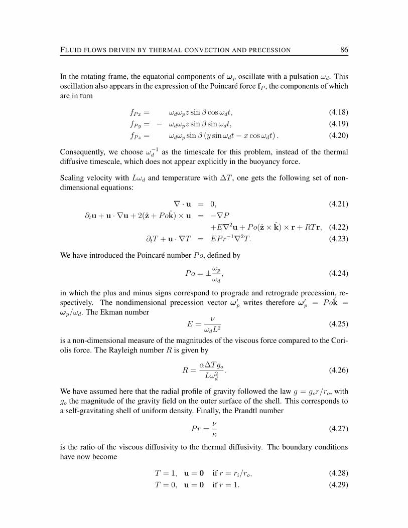
FLUID FLOWS DRIVEN BY THERMAL CONVECTION AND PRECESSION 86
In the rotating frame, the equatorial components of ωp oscillate with a pulsation ωd. Thisoscillation also appears in the expression of the Poincaré force fP , the components of whichare in turn
fPx = ωdωpz sin β cos ωdt, (4.18)fPy = − ωdωpz sin β sin ωdt, (4.19)fPz = ωdωp sin β (y sin ωdt − x cos ωdt) . (4.20)
Consequently, we choose ω−1d as the timescale for this problem, instead of the thermal
diffusive timescale, which does not appear explicitly in the buoyancy force.
Scaling velocity with Lωd and temperature with ∆T , one gets the following set of non-dimensional equations:
∇ · u = 0, (4.21)∂tu + u · ∇u + 2(z + Pok) × u = −∇P
+E∇2u + Po(z × k) × r + RTr, (4.22)∂tT + u · ∇T = EPr−1∇2T. (4.23)
We have introduced the Poincaré number Po, defined by
Po = ±ωp
ωd
, (4.24)
in which the plus and minus signs correspond to prograde and retrograde precession, re-spectively. The nondimensional precession vector ω ′
p writes therefore ω′p = Pok =
ωp/ωd. The Ekman numberE =
ν
ωdL2(4.25)
is a non-dimensional measure of the magnitudes of the viscous force compared to the Cori-olis force. The Rayleigh number R is given by
R =α∆Tgo
Lω2d
. (4.26)
We have assumed here that the radial profile of gravity followed the law g = gor/ro, withgo the magnitude of the gravity field on the outer surface of the shell. This corresponds toa self-gravitating shell of uniform density. Finally, the Prandtl number
Pr =ν
κ(4.27)
is the ratio of the viscous diffusivity to the thermal diffusivity. The boundary conditionshave now become
T = 1, u = 0 if r = ri/ro, (4.28)T = 0, u = 0 if r = 1. (4.29)
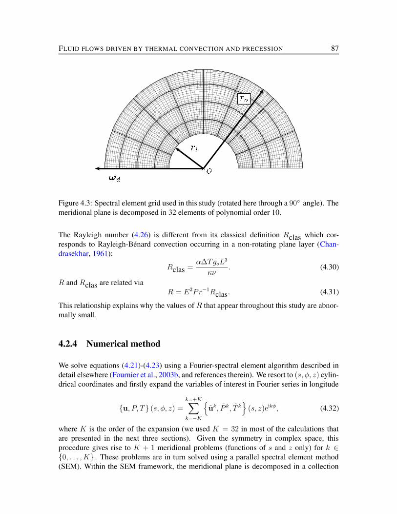
FLUID FLOWS DRIVEN BY THERMAL CONVECTION AND PRECESSION 87
¡¢¤£
¥§¦
¥©¨
Figure 4.3: Spectral element grid used in this study (rotated here through a 90° angle). Themeridional plane is decomposed in 32 elements of polynomial order 10.
The Rayleigh number (4.26) is different from its classical definition Rclas which cor-responds to Rayleigh-Bénard convection occurring in a non-rotating plane layer (Chan-drasekhar, 1961):
Rclas =α∆TgoL
3
κν. (4.30)
R and Rclas are related viaR = E2Pr−1Rclas. (4.31)
This relationship explains why the values of R that appear throughout this study are abnor-mally small.
4.2.4 Numerical method
We solve equations (4.21)-(4.23) using a Fourier-spectral element algorithm described indetail elsewhere (Fournier et al., 2003b, and references therein). We resort to (s, φ, z) cylin-drical coordinates and firstly expand the variables of interest in Fourier series in longitude
u, P, T (s, φ, z) =k=+K∑
k=−K
uk, P k, T k
(s, z)eikφ, (4.32)
where K is the order of the expansion (we used K = 32 in most of the calculations thatare presented in the next three sections). Given the symmetry in complex space, thisprocedure gives rise to K + 1 meridional problems (functions of s and z only) for k ∈0, . . . , K. These problems are in turn solved using a parallel spectral element method(SEM). Within the SEM framework, the meridional plane is decomposed in a collection

FLUID FLOWS DRIVEN BY THERMAL CONVECTION AND PRECESSION 88
of non-overlapping elements (see figure 4.3). For each Fourier mode k, uk, P k, T k areapproximated locally within each element by means of tensorized bases of polynomials ofdegree N for velocity and temperature, and N − 2 for pressure. Each meridional problemis cast in its variational form, for which the trial functions are taken to be equal to the basisfunctions we just described. More specifically, these basis functions are the tensor productof the Lagrangian interpolants defined over the Gauss-Lobatto-Legendre quadrature pointsof order N . Inside elements sharing an edge with the z axis, a weighted Gauss-Lobatto-Legendre quadrature is introduced, which incorporates the cylindrical radius in its weight,in order to avoid a potential degeneracy of the discrete set of equations due to nodes locatedon the z axis (Bernardi et al., 1999). Figure 4.3 shows a spectral element grid consistingof 32 spectral elements of degree 10, which was used for the most of the calculations pre-sented in the following.
The resulting semi-discrete problem is timestepped using a second order scheme, whichtreats the viscous and Coriolis forces implicitly and the nonlinear interactions in a fullyexplicit fashion, using the 3/2 rule (Orszag, 1971). Regarding the precessing situation ofinterest here, we should add that the extra Coriolis term 2ω ′
p × u is treated explicitly andthat the Poincaré force fP is treated implicitly thanks to its well-known expression, seeequations (4.18)-(4.20).
The resulting algebraic systems are solved using preconditioned conjugate (or biconjugate)gradient algorithms. Jacobi (diagonal) preconditioning is used to solve for velocity andtemperature, whereas a multilevel overlapping Schwarz method is used to solve for pressure(Fournier et al., 2003a). Domain decomposition is performed in the meridional plane andparallel processing is implemented following the message passing paradigm (Gropp et al.,1999).
4.2.5 Choice of parameters
Equations (4.21)-(4.23) show that the problem of interest is controlled by 6 parameters: theradius ratio ri/ro, the Ekman number E, the Poincaré number Po, the angle β, the Rayleighnumber R, and the Prandtl number Pr. These define a very wide parameter space, and weshall in the following fix the radius ratio to .35, the Ekman number to 10−3, the Prandtlnumber to 1, and β to π/2. A radius ratio of .35 corresponds to today’s Earth radius ratio(Yoder, 1995). The Ekman number we choose is larger by several orders of magnitude to itsEarth value of O(10−12), based on different estimates of the viscosity of liquid iron undercore conditions (Poirier, 1988; de Wijs et al., 1998). Taking 10−3 is not entirely foolishthough, since flows computed for this number already exhibit characteristic properties ofrapidly rotating flows, such as narrow Ekman boundary layers, whose thickness goes likeE1/2L (see e.g. Greenspan, 1990). Moreover, dealing with a neutral fluid, and therebyomitting to consider any magnetic effects, we can as well set the value of Pr to 1, insteadof the O(10−2) value appropriate for liquid metals (Gubbins & Roberts, 1987).

FLUID FLOWS DRIVEN BY THERMAL CONVECTION AND PRECESSION 89
Regarding the value of β, let us first split the dimensionless precession vector ω ′p into its
component parallel to the axis ω′pz and its equatorial component ω′
pxy
ω′p = ω′
pz + ω′pxy. (4.33)
The Coriolis force fC and the Poincaré force fP can now be written
fC = −2(z + ω′pz + ω′
pxy) × u, fP = (z × ω′pxy) × r. (4.34)
As long as Po is sufficiently small so that ω′pz can be neglected with respect to z, the main
effect of precession is due to the action of the equatorial component of the precession vectorω′
pxy, the amplitude of which is given in nondimensional units by Po sin β , see equations(4.15)-(4.17). In this respect, all the (β, Po) pairs corresponding to the same Po sin β areequivalent. We therefore choose to set β = π/2 and have Po vary.
4.3 Convection without precession
Being left with two free parameters, we make matters even simpler in this section by re-stricting our attention to purely convective flows, by varying R and setting Po to 0. Asstated in the introduction, the convective end member of our problem has received consid-erable attention in the past (Gubbins & Roberts, 1987, and references therein). The goalof this section is to recall the main properties of rotating, convective flows and to define areference convective state for the convecto-precessing calculations of section 4.5.
4.3.1 Critical Rayleigh number
First of all, we wish to determine the so-called critical Rayleigh number Rc. It correspondsto a critical temperature difference ∆T maintained across the shell, for which thermalconduction is not efficient enough in removing heat from the fluid; convective currentsdevelop in order to get rid of the excess heat. In a milestone paper, Busse (1970) studied theassociated linearized problem and showed that the convective instability took the form of adrifting sequence of columns parallel to the axis of rotation, located at a given cylindricalradius. The columns are alternatively hot and cold, relative to the conductive temperatureprofile. They correspond to a thermal Rossby wave, which propagates in the progradedirection in the case of a sphere. The dependence of the critical longitudinal wavenumberkc and the angular velocity of the wave on E and Pr has have been studied in sphericalgeometry by several authors (see e.g. Yano, 1992; Jones et al., 2000). The main idea is thatones gets an increasing number of pairs as the Ekman number is decreased: for the viscousforce to have a substantial effect in the force balance (and eventually induce a secondary,non-geostrophic convective flow), decreasing E makes it necessary for velocity gradientsto be localized over shorter and shorter scales.

FLUID FLOWS DRIVEN BY THERMAL CONVECTION AND PRECESSION 90
0 1 2 3 4 5 60.00
0.02
0.04
0.06
0.08
0.10
0.12
0.14
0.16
ª
«T¬ ®¯° ±³²µ´A°¶· ¸º¹6·»½¼·¾¿ ¸º¹¸½ÀCÁm¿Âà ¸º¹¸½ÁCÁ·¾Â ¸º¹¸½ÀC¸CÀ)» ¸º¹6·I¸m¿C»)À¼ ¸º¹6·¿½¸m¿Â
Figure 4.4: Numerically determined value of the critical Rayleigh number Rc(k) forFourier modes ranging from k = 1 to k = 6. The curve reaches its minimum for k = 3which is the critical azimuthal wavenumber. Values of Rc(k) are also tabulated for refer-ence.
In our case, for a moderately small E = 10−3, we expect the scale of these instabilities tobe quite large, and consequently a small value for kc.
The determination of kc is done in a trial and error fashion: the set of governing equations(4.21)-(4.23) is linearized about the basic, conductive state. For a given Fourier modek, we start from a random meridional temperature distribution, and the linearized set istimestepped for different values of R. The growth rate σ(k) of the instability is monitored,which enables to determine the value of Rc(k) – defined by the marginal condition σ(k) =0 – by dichotomy.
The critical Rayleigh number Rc is given by
Rc = mink
Rc(k). (4.35)
Results obtained following this procedure are plotted on figure 4.4, for k ∈ 1, . . . , 6.The critical convective mode has a threefold symmetry in longitude and is obtained for aRayleigh number of 0.08817, or equivalently Rclas = 8.817 104.

FLUID FLOWS DRIVEN BY THERMAL CONVECTION AND PRECESSION 91
ÄÆÅÈÇÉ+ÊËÄÍÌ ÄÆÅÏÎÐÉ0ѧÄÒÌ ÄÆÅÔÓÕÉ+ÊËÄÍÌÖ × Ø
Ù Ú Û
Ü Ý Þ
ß à á
Figure 4.5: From top to bottom: Temperature deviation in the equatorial plane, z-component of vorticity in the equatorial plane, radial velocity at mid-depth, as seen from theNorth pole, and mean zonal flow in the northern hemisphere. Results obtained for R = 1.7,3.4 and 5.7 Rc (from left to right). All plots are normalized. Solid lines (red regions) anddashed lines (blue regions) represent positive and negative values, respectively.

FLUID FLOWS DRIVEN BY THERMAL CONVECTION AND PRECESSION 92
4.3.2 Finite amplitude convection
Introduction
Fully nonlinear solutions to the rotating convection problem are computed starting froman initial temperature perturbation having the critical, threefold symmetry in longitude,and a zero velocity field. Calculations are carried out until a steady, or quasi-steady stateis reached. We consider a quasi-steady state realized when the running average F ofa given field f , defined by F (t) = (1/t)
∫ t
0f(t′)dt′, has converged. In what follows,
three distinct and representative Rayleigh numbers will be considered, corresponding to1.7, 3.4, and 5.7Rc. We will refer to the temperature deviation, T − Tcond, in whichTcond is the static, conductive radial temperature profile
Tcond(r) =ri
ro − ri
[ro
r− 1]
. (4.36)
A quick tour of rotating convective flows
Several snapshots of interest are displayed on figure 4.5. Each column corresponds to agiven Rayleigh number. From top to bottom, we plot the temperature deviation in theequatorial plane z = 0, the z-component of the vorticity ∇ × u in the equatorial plane, aview from the North pole of the radial velocity at mid-depth, and the mean zonal flow u0
φ.The first two snapshots aim at describing the the potential periodicity of the characteristicpatterns of the flow, while the radial velocity contours should provide additional informa-tion on the transport of heat at work in the shell. Finally, the mean zonal flow providesan extra meridional information on the overall circulation of the fluid and in particular, itcould reveal the existence of differential rotation.
• R = 1.7Rc: For this value of R, the solution reaches a steady state and keeps itsoriginal threefold symmetry in longitude. As can be seen on figure 4.5a, the tem-perature anomalies are located in large Busse rolls, located outside of the tangentcylinder C, the imaginary cylinder that circumscribes the inner sphere and is parallelto the axis of rotation. Figure 4.5d shows that the mean zonal flow is mostly concen-trated in tropical latitudes, meaning that there is very little activity occurring in C.Figure 4.5c outlines the fact that radial flow (and hence heat transport) is accordinglyconcentrated in the equatorial regions.
The shape of the Busse rolls does not vary with time, and the solution is steady, exceptfor a retrograde azimuthal drift ωb = −1.39 10−3. In finite amplitude convection, theslope of the spherical boundary induces via the nonlinear term u · ∇u a retrogradezonal wind which can eventually overcome the prograde propagation of the thermalRossby waves (e.g. Cardin & Olson, 1994), and this is what is happening here. The

FLUID FLOWS DRIVEN BY THERMAL CONVECTION AND PRECESSION 93
spiraling aspect of the contours is related to the slope of the spherical boundary be-ing steeper and steeper as one approaches the outer boundary of the shell. For adetailed analysis of this effect, the reader is referred to Jones et al. (2000). Vorticitycontours (figure 4.5b) indicate that the maximum vorticity is located inside the innerEkman boundary layers. We can still discern three pairs of cyclones and anticyclonesin the bulk of the shell. Cyclonic motion draws fluid from the northern and south-ern hemisphere into the equator, following a mechanism similar to Ekman suction(Greenspan, 1990), while anticyclones expel fluid from the equator. This explainswhy the cyclones are in comparison wider than the anticyclones.
• R = 3.4Rc: Increasing the Rayleigh number, the spiraling effect becomes strongenough to break the Busse rolls, and this ultimately generates a sixfold symmetry inlongitude (figures 4.5e and 4.5f). The shape of the resulting structures vary with timeand the solution is strongly time-dependent. In order to get a better idea of the fluctu-ations of the flow, we plot on figure 4.6 (top) the modal kinetic energy ek
kin containedin the k = 3 and k = 6 modes with respect to time, in the [500,1000] dimensionlesstime window. k = 6 is clearly dominant over time, but there are occasional periodsof time, such as the [700,800] interval, during which the original threefold symmetryis recovered. Even if it now occurs on a k = 6 azimuthal lengthscale, heat transportis still concentrated in equatorial regions, as can be seen on figure 4.5g. Furthermore,we note the presence of some activity inside C, as differential rotation is now visibleon figure 4.5h.
• R = 5.7Rc: Increasing the Rayleigh number even further, one might expect an evenmore chaotic situation. On the contrary, we note on figure 4.5i that the flow seems,on least on this snapshot, to have recovered in part its original symmetry. Cold,k = 3, thermal anomalies are concentrated around the inner core (in a region wherethe spiraling effect is small). Furthermore, the outer, hot anomalies are not slicedinto two distinct halves. The restored threefold symmetry is also noticeable on thevorticity contours (figure 4.5j), where three equatorial anticyclones are visible. Weattribute this change in morphology to the existence of a polar transport of heat (figure4.5k) which has a threefold symmetry and stabilizes the equatorial flow. This polarstabilization effect is also seen on figure 4.6 (bottom): the k = 3 mode is now roughlythree times more energetic than the k = 6 mode, and, interestingly enough, the timedependence has a pronounced oscillatory character. Zonal winds (figure 4.5l) areconcentrated inside C: this is yet another manifestation of a major change in thecharacter of convection. The development of a polar circulation when a sufficientlysupercritical Rayleigh number is prescribed has already been observed in numericalsimulations, for instance by Tilgner & Busse (1997).

FLUID FLOWS DRIVEN BY THERMAL CONVECTION AND PRECESSION 94
0.0
5.0×10⁻⁵
1.0×10⁻⁴
1.5×10⁻⁴
2.0×10⁻⁴
500 600 700 800 900 10000
1×10⁻⁴
2×10⁻⁴
3×10⁻⁴
4×10⁻⁴
5×10⁻⁴ âãä å æâçä å æ
èé ê©ë
ìîíïñðòôó,õTó.ö÷øxó.ù,úûýüÿþ û
ìîíïñðòôó,õTó.ö÷øxó.ù,úûýü û
Figure 4.6: Timeseries of modal kinetic energy ekkin contained in modes k = 3 (dashed
line) and k = 6 (solid line) for R = 3.4Rc (top) and R = 5.7Rc (bottom).
Reference convective state
From the three cases considered above, it appears that the structure of a rotating convectiveflow becomes more and more interesting (and complicated) as we increase the Rayleighnumber R, a noteworthy feature being the development of polar convection currents.
For simplicity (and computational convenience), we shall ignore time-dependent flows andrestrict our attention to the R = 1.7Rc case, which is steady (aside from its azimuthal drift),and define this convective state as the reference convective state, bearing in mind that thisflow is characterized by large-scale equatorial features.
The reference convective state sets the initial conditions for the problem which mixes boththe effects of precession and thermal convection, which we address in section 4.5. Beforethis, we will review the basic properties of precession-driven flows (setting R = 0 andignoring thermal effects) in the next section.

FLUID FLOWS DRIVEN BY THERMAL CONVECTION AND PRECESSION 95
4.4 Basic precessing flows
4.4.1 Reference studies
The problem of precession-driven flows in a fluid embedded in a rigid container was firstconsidered by Poincaré (1910) and a summary of his work can be found for instance inLamb (1932); Rochester et al. (1975); Malkus (1994). Working in the precessing frame(the frame rotating at ωp only), Poincaré showed that the inviscid steady flow driven insidethe cavity was a flow of constant vorticity, corresponding to a rigid rotation of the fluidabout a rotation vector ωf , the orientation of which is controlled by the precession rate(viz. the Poincaré number Po), and the ellipticity of the container e. For a small Po, theangle χ between ωd and ωf is given by (Rochester et al., 1975, equation (23))
χ ≈ Po sin β
e, (4.37)
an expression which becomes singular in the spherical case e = 0. This singularity canbe explained by considering the mechanism responsible for the coupling between the rigidcontainer and the fluid, namely the hydrodynamic pressure torque imposed on the fluid bythe container on the ellipsoidal boundary. This torque vanishes in the spherically symmetriccase, and viscous effects must be introduced in order for the fluid to be coupled to thecontainer.
In another of his milestone papers, Busse (1968) solved the same problem for a viscousfluid, extending the boundary layer formulation of Stewartson & Roberts (1963) to thetreatment of the nonlinear terms in the boundary layer equation. Working in the precessingframe also, he derived an implicit expression for ωf , which writes in the spherical case
ωf = zω2f +
z × ω′p
(
2.62(Eωf )1/2)
+ z × (ω′p × z)ω2
f
(
0.259(E/ωf )1/2 + ω′
p · z)
2.622Eωf +(
0.259(E/ωf )1/2 + ω′p · z
)2 ,
(4.38)in which E is the Ekman number. Busse found this expression following a rather convo-luted scheme, seeking the solution as an expansion in powers of E1/2. More recently, Noiret al. (2003) derived the same expression following a much simpler argument based upona torque balance between precessional, pressure, and viscous torques.
The peculiar coefficients that appear in equation (4.38) originate from the excitation of theso-called spinover mode of the sphere by the Poincaré force. The spinover mode representsa rigid rotation about an axis other than the rotation axis of the sphere (or spheroid). Aspointed out by Greenspan (1990), “it is the easiest mode to excite, for all that is required isa slight impulsive change in the direction of the rotation axis of a rigidly rotating sphere".This k = 1 mode is definitely excited by the precession of the container, and it appears inthe analysis of Noir et al. (2003) in the calculation of the viscous torque: 0.259E1/2 and

FLUID FLOWS DRIVEN BY THERMAL CONVECTION AND PRECESSION 96
2.62E1/2 are in fact the nondimensional frequency and decay rate of the viscously modifiedspinover mode, respectively.
4.4.2 Basic precessing flows in a spherical shell
In our case, the presence of an inner core of substantial size complicates matters a little bit,and no analytical solution exists for this configuration. We should however retrieve similarflow patterns. To confirm this, we computed using our numerical code the steady solutionobtained for a Poincaré number of 0.01, starting from a zero initial velocity field (again,thermal effects are not considered here). The flow reaches a steady state within a fewspinup times; on figure 4.7a, we plot a collection of three-dimensional isosurfaces of thekinetic energy density of the solution, in the precessing frame. In this frame, the solutioncorresponds to a flow of almost uniform vorticity, whose rotation vector ωf is slightly tiltedwith respect to the z axis. Departure from uniform vorticity occurs in the Ekman boundarylayers and is visible through a kink in the isosurfaces near the outer boundary. If we nowexpress this solution in our working frame (figure 4.7b), we find that it is no longer steadyand seems to be now associated with a solid-body rotation organized around a vector ωeq
located on the equator. This axis rotates about the z axis with a nondimensional unityretrograde angular velocity, as it follows ω ′
p – see equations (4.15)-(4.17). Note that to plotfigure 4.7b, we have removed the outer Ekman boundary layers, which would otherwisemask the inner cylinders.
In order to get a better understanding of the flow, we provide on figure 4.8a a view of thevertical velocity uz in the equatorial plane, looking from the north pole. We observe oneupwelling and one downwelling owing to the cylindrical symmetry that is exhibited on 4.7b.The inner core manifests itself through the Ekman layer that is generated in its vicinity. Onfigure 4.8b, we show for completeness the solution to the same problem obtained in a fullsphere. We note that outside of the inner Ekman layer, the two solutions are in very closeagreement. In both cases, they exhibit a k = 1 symmetry in longitude. Figures 4.8a and bcan be interpreted as images of the viscously modified spinover mode in a spherical shelland in a sphere, respectively. The flow is not, however, exactly organized as a solid bodyrotation around a global ωeq; a more precise description could be obtained for instance byconsidering ωeq a function of the radius r.
Precession-driven flows is a wide topic, which goes well beyond the simple description wehave made here. Of particular interest are the actual limits of validity of formula (4.38).Tilgner & Busse (2001) made a systematic study of precession-driven flows in a sphericalshell with a minuscule inner core (for numerical commodity), and they found that equation(4.38) was in fact valid for a range of (Po, β) broader than expected. Nevertheless, forlarge values of Po, the angle between ωf and z becomes too large, which can triggerhydrodynamic instabilities. On figure 4.9, we plot the vertical velocity uz in the equatorialplane for obtained for Po = 0.001, 0.01, and 0.1, once the solid body component ωeq × r

FLUID FLOWS DRIVEN BY THERMAL CONVECTION AND PRECESSION 97
! "#
$% &' ")(+*,-
Figure 4.7: a: Kinetic energy density isosurfaces of steady precessing flow correspondingto Po = 0.01. The three Cartesian axes are color coded, red is (Ox), green is (Oy), andblue is (Oz). The solution is displayed here in the precessing frame, which is the framerotating at ω′
p. It is steady in this frame. b: same plot for the solution now seen fromthe frame rotating at ω′
p + z (our working frame). In this frame, the solution correspondsroughly to a solid-body rotation organized around an axis located in the equator and it is notsteady, as this axis rotates about the z axis with a nondimensional unity retrograde angularvelocity. We have removed on this plot the outer Ekman boundary layer.
. /
Figure 4.8: a: Isocontours and isosurfaces of vertical velocity uz of steady precessingflow in a spherical shell in the equatorial plane, looking from the north pole. Red regionsand solid lines for positive uz, blue regions and dashed lines for negative uz. This plotcorresponds to the flow displayed on figure 4.7b. Red and green lines correspond to (Ox)and (Oy) axes, respectively. b: same plot for flow obtained in a full sphere for the samevalue of the Poincaré number (0.01).
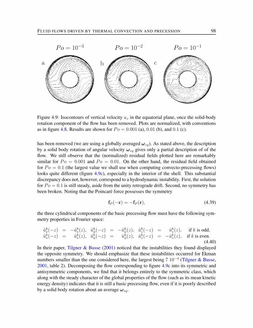
FLUID FLOWS DRIVEN BY THERMAL CONVECTION AND PRECESSION 98
a b c
Po = 10−3
Po = 10−2
Po = 10−1
Figure 4.9: Isocontours of vertical velocity uz in the equatorial plane, once the solid-bodyrotation component of the flow has been removed. Plots are normalized, with conventionsas in figure 4.8. Results are shown for Po = 0.001 (a), 0.01 (b), and 0.1 (c).
has been removed (we are using a globally averaged ωeq). As stated above, the descriptionby a solid body rotation of angular velocity ωeq gives only a partial description of of theflow. We still observe that the (normalized) residual fields plotted here are remarkablysimilar for Po = 0.001 and Po = 0.01. On the other hand, the residual field obtainedfor Po = 0.1 (the largest value we shall use when computing convecto-precessing flows)looks quite different (figure 4.9c), especially in the interior of the shell. This substantialdiscrepancy does not, however, correspond to a hydrodynamic instability. First, the solutionfor Po = 0.1 is still steady, aside from the unity retrograde drift. Second, no symmetry hasbeen broken. Noting that the Poincaré force possesses the symmetry
fP (−r) = −fP (r), (4.39)
the three cylindrical components of the basic precessing flow must have the following sym-metry properties in Fourier space:
uks(−z) = −uk
s(z), ukφ(−z) = −uk
φ(z), ukz(−z) = uk
z(z), if k is odd,uk
s(−z) = uks(z), uk
φ(−z) = ukφ(z), uk
z(−z) = −ukz(z), if k is even.
(4.40)In their paper, Tilgner & Busse (2001) noticed that the instabilities they found displayedthe opposite symmetry. We should emphasize that these instabilities occurred for Ekmannumbers smaller than the one considered here, the largest being 7 10−4 (Tilgner & Busse,2001, table 2). Decomposing the flow corresponding to figure 4.9c into its symmetric andantisymmetric components, we find that it belongs entirely to the symmetric class, whichalong with the steady character of the global properties of the flow (such as its mean kineticenergy density) indicates that it is still a basic precessing flow, even if it is poorly describedby a solid body rotation about an average ωeq.

FLUID FLOWS DRIVEN BY THERMAL CONVECTION AND PRECESSION 99
Table 4.1: Ratio of the mean kinetic energy ekin of convecto-precessing flows to the meankinetic energy of the reference convective state e0
kin.
Po 0.005 0.01 0.03 0.05 0.08 0.1
ekin/e0kin 6.60 23.3 1.92 102 4.85 102 1.01 103 1.32 103
4.5 Precession and convection
Having in mind the basic properties of convection-driven and precession-driven flows, wenow turn to the full problem of flows driven by these two phenomena at the same time. Asstated in section 4.3.2, the initial conditions are defined by the convective solution obtainedfor R = 1.7Rc. We shall consider 6 different Poincaré numbers here: 0.005, 0.01, 0.03,0.05, 0.08, and 0.1 – all cases reflect a prograde precession of the shell. Precession isimpulsively turned on, and the model is run until a new quasi-steady state is obtained.
4.5.1 Velocity fields
We begin by looking at the mean kinetic energy ekin characterizing the set of solutions. Ontable 4.1, they are given as a function of the Poincaré number and normalized with respectto the mean kinetic energy e0
kin of the initial conditions. The mean kinetic energy ekin isalways larger than e0
kin, by one up to three orders of magnitude. The reference convectivestate being only slightly supercritical, its weight is negligible compared to the input thatoriginates from the Poincaré force, even for small values of Po. The various velocity fieldsobtained resemble closely the ones depicted in the previous section. As a matter of fact,when we increase the Poincaré number, the morphology of the velocity field evolves fromthe one depicted on figures 4.7b, 4.9a and 4.9b to the one corresponding to figure 4.9c.Having described these fields previously, we will focus on temperature in the remainder ofthis section.
4.5.2 Temperature fields
On figure 4.10, we plot the temperature spectra S(k), defined by
S(k) =1
2V (2K + 2)2
∫
Ω
|T k|2sdsdz, (4.41)

FLUID FLOWS DRIVEN BY THERMAL CONVECTION AND PRECESSION 100
0 1 2 3 4 5 6 7 8 9
1×10⁻⁷
1×10⁻⁶
1×10⁻⁵
1×10⁻⁴
1×10⁻³
1×10⁻²
1×10⁻¹
0213415617981
:;=<?>A@CB:;<?>9@ >9B:;<?>9@ >ED:;<?>9@ >F>FD:;<?>9@ >FG:;<?>9@ >FH
IJ KL
M
Figure 4.10: Temperature spectra (truncated at k = 9) for convecto-precessing flows.The spectrum of the initial convective state is represented with large empty circles, whileconvecto-precessing solutions are displayed with solid symbols of varying color and shape.

FLUID FLOWS DRIVEN BY THERMAL CONVECTION AND PRECESSION 101
where V is the volume of the shell, and Ω denotes the meridional plane. The (2K + 2)2
factor in the denominator originates from the normalization of the discrete fast Fouriertransform used in the simulation (Frigo & Johnson, 1997). T k in equation (4.41) is thetotal temperature (not the temperature deviation); accordingly, the temperature spectrumis dominated in all cases by the axisymmetric temperature mode, whose energy remainsconstant to within 1% when the Poincaré number is increased. Leaving this mode aside, wenotice not surprisingly that the reference spectrum (plotted with large circles) is dominatedby the k = 3 mode. As seen in section 4.3, the Busse rolls are a stable feature, and very littleenergy is found in the harmonics (less than 2.5% of the total non-axisymmetric energy).As soon as Po > 0, the velocity field is dominated by its order 1 component (see section4.4.2). The nonlinear term in the heat equation (4.23) couples each temperature mode kwith modes k ± 1, thereby populating the entire spectrum. When Po ≤ 0.05, most of thenon-axisymmetric energy is nevertheless still confined in the k = 3 mode. The Busse rolls,which are almost stationary in space (|ωb| = 1.39 10−3 1), are not really sensitive tothe equatorial solid-body rotation which characterizes the precession-dominated flow. Thedrift of the cylindrical motion is too fast to have a net effect on the temperature patterns.Roughly speaking, a given Busse roll is not given enough time to wrap itself around therotating equatorial cylinder. What is happening here is in essence similar to the argumentthat led Rochester et al. (1975) to contest Malkus’ view: when (correctly) envisioned in theframe rotating at z + ω′
p, a laminar precessing flow does not have a substantial, permanenteffect.
Figures 4.11a and 4.11b show isosurfaces of non-dimensional temperature deviations of±0.2 (red for hot, blue for cold) obtained for Po = 0.01 and 0.05, respectively. Bytemperature deviations, we still mean deviation from the conductive profile (4.36), evenif there is no static, conductive solution to the convecto-precessing problem, due to thenon-conservative character of the Poincaré force. However, looking at departures fromthis hypothetical state eases the understanding of the results and their comparison with thepurely convective situation. In both cases, the k = 3 symmetry is preserved. The Busserolls have been rotated with respect to a rotation axis located in the equator, the inclinationbeing more pronounced for Po = 0.05 (figure 4.11b).
It takes quite a large value of Po for the original symmetry to be at least partially lost. Asindicated on figure 4.10, mode k = 3 is no longer dominant for Po = 0.08 and Po =0.1. For Po = 0.08, modes k = 1, 2, 3 are equally energetic, while mode k = 1 isdominant for Po = 0.1. Figure 4.11c (Po = 0.08) reveals that secondary cold featureshave appeared. Three small hot regions can be seen which fill the space between coldregions. For Po = 0.1 (figure 4.11d), cold anomalies are now predominantly of order 2;the three hot anomalies of figure 4.11c have become a pair of substantially larger size.

FLUID FLOWS DRIVEN BY THERMAL CONVECTION AND PRECESSION 102
N O
P Q
Figure 4.11: Isosurfaces of temperature deviations of amplitude ±0.2 (red for hot, blue forcold) for convecto-precessing flows computed for Po = 0.01 (a), 0.05 (b), 0.08 (c) and 0.1(d). Axes color-coded as in figure 4.7.
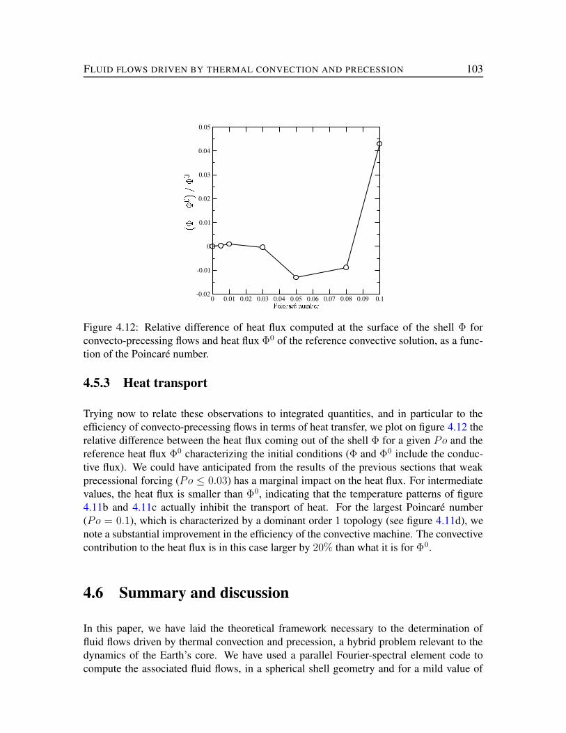
FLUID FLOWS DRIVEN BY THERMAL CONVECTION AND PRECESSION 103
0 0.01 0.02 0.03 0.04 0.05 0.06 0.07 0.08 0.09 0.1-0.02
-0.01
0
0.01
0.02
0.03
0.04
0.05
R SUTSV W XSV
YUZ\[ ]^6_\`bac ]bdfehg c `Figure 4.12: Relative difference of heat flux computed at the surface of the shell Φ forconvecto-precessing flows and heat flux Φ0 of the reference convective solution, as a func-tion of the Poincaré number.
4.5.3 Heat transport
Trying now to relate these observations to integrated quantities, and in particular to theefficiency of convecto-precessing flows in terms of heat transfer, we plot on figure 4.12 therelative difference between the heat flux coming out of the shell Φ for a given Po and thereference heat flux Φ0 characterizing the initial conditions (Φ and Φ0 include the conduc-tive flux). We could have anticipated from the results of the previous sections that weakprecessional forcing (Po ≤ 0.03) has a marginal impact on the heat flux. For intermediatevalues, the heat flux is smaller than Φ0, indicating that the temperature patterns of figure4.11b and 4.11c actually inhibit the transport of heat. For the largest Poincaré number(Po = 0.1), which is characterized by a dominant order 1 topology (see figure 4.11d), wenote a substantial improvement in the efficiency of the convective machine. The convectivecontribution to the heat flux is in this case larger by 20% than what it is for Φ0.
4.6 Summary and discussion
In this paper, we have laid the theoretical framework necessary to the determination offluid flows driven by thermal convection and precession, a hybrid problem relevant to thedynamics of the Earth’s core. We have used a parallel Fourier-spectral element code tocompute the associated fluid flows, in a spherical shell geometry and for a mild value of

FLUID FLOWS DRIVEN BY THERMAL CONVECTION AND PRECESSION 104
the Ekman number (10−3).
For this value, and a reference convective state obtained choosing a Rayleigh number 1.7times critical, calculations indicate that, to first order, convection and precession ignoreeach other. In the cases considered here, the velocity field is primarily a k = 1 precession-induced field, of unity retrograde drift, and it affects only marginally the k = 3 temperaturepatterns (and related heat transport).
It takes a large value of the Poincaré number for the (almost) stationary Busse rolls thatdefine the reference convective state to be altered by the precessing flow, and for convectivetransport to be enhanced by precession. This happens in situations for which the flowis substantially different from a solid-body rotation organized around an equatorial axis.We would like to emphasize again that the flow is still stable and that no hydrodynamicinstability is present, due to the large value of the Ekman number.
Having chosen a steady convective pattern –the only time-dependence is the retrogradedrift of the rolls ωb, whose amplitude is 1, 000 times smaller than the drift of the precessingflow–, we have set ourselves in the worst case situation in terms of timescales discrepancy.This shows the need to repeat this first exercise for time-dependent reference convectivestates, corresponding for instance to R = 5.7Rc (§4.3). Using a more supercritical valueof R, the flow is characterized by timescales closer to the rotation period, see figure 4.6(bottom). This observation, along with the new morphology of convection (figures 4.5kand 4.5l), suggests that the interaction of precession with convection will, in this case,bring up new interesting physics with respect to the situations we have considered in thispaper. The computational price to pay to study this regime is not too expensive in termsof resolution: to compute the convective solution for R = 5.7Rc, we used the mesh offigure 4.3, taking (N = 13, K = 32) –instead of (N = 10, K = 32) for R = 1.7Rc. Thecost comes really from the need for long integration times to perform accurate statistics,but it is not prohibitive (we are currently investigating this new regime).
Another path to explore is the one going toward an Earth-like situation, by addressing thesame problem for smaller values of the Ekman number. On figure 4.13, we have reproduced(on a log scale) the critical Rayleigh number curve of figure 4.4 and added the same curveobtained for E = 10−4 (shown with diamonds). The critical Fourier mode is now the k = 6mode, indicating that a convective flow develops smaller scales as the Ekman number isdecreased. This broadens the spectral gap between the Poincaré force and the buoyancyforce, and should reveal a wide variety of flow behaviors.
Also, for smaller values of E, precessing flows are more prone to instabilities (Tilgner& Busse, 2001; Lorenzani & Tilgner, 2001). In their paper, Lorenzani & Tilgner (2001)report one instability occurring at E = 10−4 for Po = −0.05 and β = 40 °(Po sin β =−0.032). Quite interestingly, they report that instabilities at E = 10−4 have predominantlya k = 7 and k = 8 azimuthal periodicity, a region in Fourier space that overlaps withthe convective instability spectrum (figure 4.13), suggesting that the basic convective flow

FLUID FLOWS DRIVEN BY THERMAL CONVECTION AND PRECESSION 105
Figure 4.13: Critical Rayleigh number as a function of Fourier mode k for E = 10−3
(circles) and 10−4 (diamonds).
might actually trigger a new kind of convecto-precessing instabilities. Related calculationshave a tremendous computational cost but they are within the reach of our code.
It is crucial to perform a systematic survey of the (numerically attainable) parameter spacebefore even attempting to say anything about what could happen in the Earth’s core. Inparticular, the trend we will get when decreasing the Ekman number is particularly impor-tant. E for the core is estimated between 10−12 and 10−15. The value for Po and β are−10−7 and 23.5 °, respectively. We can not reject the possibility a turbulent flow of preces-sional origin, potentially able to power the dynamo, only on the basis of the smallness ofPo. Ideally, we would like to map out the changes in flow properties as we vary the triplet(E,Po,R).
This unexplored and promising problem must ultimately incorporate two effects to be rele-vant for the Earth. First, magnetic effects have to be included. This is not a trivial task, andwe just started to work on the implementation of the related induction equation followinga Fourier-spectral element methodology. Second, the ellipticity e of the outer boundary(1/373 at the core-mantle boundary) should be taken into account. Noir et al. (2003) showthat the pressure torque coupling the rigid container and the fluid is proportional to e, whilethe viscous torque is proportional to E1/2. In the Earth, the latter is consequently smallerthan the former. The geometrical flexibility of our numerical approach enables to considerboundaries of arbitrary ellipticity, since there is no constraint on the shape of the merid-ional section of the computational domain (Fournier et al., 2003a). For values of the Ekmannumber in the 10−3−10−4 range, values of e in the 0−0.3 range will have to be considered.
Chapter 5
Afterwords
The discussion of chapter 4 outlined the interest of pursuing the study of convecto-precessingflows, by exploring the parameter space more systematically. Highly supercritical convec-tion should be considered, along with higher rotation rates (smaller Ekman numbers) inorder to get closer to the Earth’s core regime. Also, the ellipticity of the core-mantle bound-ary should be taken into account and the spherical shell assumption relaxed. The flexiblenumerical approach we have presented in this thesis will enable this, but, beforehand, wewill have to optimize our code. Not a rewarding exercise for an apprentice geophysicistdeveloping a numerical model from scratch, optimization is a key issue to address in or-der to get anywhere close to interesting geophysical regimes, as was proved in the past forinstance by Bunge & Baumgardner (1995) and Clune et al. (1999).
Once this task has been performed, future work will focus on turning this hydrodynamiccode into a magnetohydrodynamic one. The equation governing the evolution of the mag-netic field (termed the induction equation) is similar to the Navier-Stokes equation, but theboundary conditions that must be prescribed are different. As a matter of fact, the magneticfield at the core-mantle boundary must be connected to an exterior potential field which de-cays to zero at infinity. This connection is straightforward if one uses spherical harmonics(Glatzmaier, 1984), but is less amenable to a local method. It can still be achieved throughthe projection of the spectral element solution onto the basis of spherical harmonics, whichcan be performed rigorously via the introduction of a Dirichlet-to-Neumann (DtN) operator–Chaljub & Valette (2003) successfully applied this technique to model the propagation oflow-frequency seismic waves at the global scale. The DtN formalism is readily applicableto the induction equation, and holds great promise for future applications of the researchpresented in this thesis.
106

Appendix A
Quadrature formulas and polynomialinterpolation
Throughout this appendix, Λ refers to [−1, +1]. The majority of the relationships thatfollow are from Bernardi et al. (1999) and Deville et al. (2002). Formula (A.21) is ourown.
A.1 Orthogonal polynomials in L2(Λ)
Let us denote the Legendre polynomials of order N with LN . The Legendre polynomialsare orthogonal in L2(Λ), that is
∀(N1, N2),
∫
Λ
LN1(ξ)LN2
(ξ)dξ =
0 if N1 6= N2
1/(N1 + 1/2) if N1 = N2(A.1)
They satisfy the conditions LN(1) = 1 and LN(−1) = (−1)N . Each LN satisfies thefollowing differential equation:
((
1 − ξ2)
L′N
)′+ N(N + 1)LN = 0. (A.2)
Legendre polynomials are computed by means of the induction formula
L0(ξ) = 1 and L1(ξ) = ξ,(N + 1)LN+1(ξ) = (2N + 1)ξLN(ξ) − NLN−1(ξ), N ≥ 1.
(A.3)
A.2 Standard Gauss-Lobatto-Legendre formula
We recall here the main properties of the standard Gauss-Lobatto-Legendre formula. Let usset ξN
0 = −1 and ξNN = 1. Then there exists a unique set of N −1 nodes ξN
i , 1 ≤ i ≤ N −1
107

QUADRATURE FORMULAS AND POLYNOMIAL INTERPOLATION 108
in Λ and of N +1 weights ρNi , 0 ≤ i ≤ N , such that the following exactness property holds
∀Φ ∈ P2N−1(Λ),
∫ 1
−1
Φ(ξ)dξ =N∑
i=0
ρNi Φ(ξN
i ). (A.4)
The ξi, 1 ≤ i ≤ N − 1 are the zeroes of L′N and the ρN
i can be expressed as follows
ρNi =
2
N(N + 1)L2N(ξN
i ), 0 ≤ i ≤ N. (A.5)
A basis for PN is made of the Lagrangian interpolants hNi , 0 ≤ i ≤ N given by
hN0 (ξ) = (−1)N−1 (1 − ξ)L′
N(ξ)
N(N + 1), (A.6)
hNi (ξ) =
1
N(N + 1)LN(ξNi )
(1 − ξ2)L′N(ξ)
ξNi − ξ
, 1 ≤ i ≤ N − 1, (A.7)
hNN(ξ) =
(1 + ξ)L′N(ξ)
N(N + 1). (A.8)
The derivatives of these interpolants, which appear for instance in the divergence and theLaplacian bilinear forms can be estimated using equation (A.2). They are given by
h′i(ξj) =
LN (ξj)
LN (ξi)1
ξj−ξii 6= j,
−N(N+1)4
i = j = 0,
N(N+1)4
i = j = N,
0 otherwise.
(A.9)
We can derive as well the pressure basis functions as the set of Lagrangian interpolantshN−2
i defined by the interior Gauss-Lobatto points ξNi , 1 ≤ i ≤ N − 1:
hN−2i (ξ) =
1 − ξNi
2
N(N + 1)LN(ξNi )
L′N(ξ)
ξNi − ξ
, 1 ≤ i ≤ N − 1. (A.10)
A.3 Orthogonal polynomials in L21(Λ)
The weighted quadrature we use is based upon a class of polynomials MN defined by
MN(ξ) =LN(ξ) + LN+1(ξ)
1 + ξ, N ≥ 0. (A.11)

QUADRATURE FORMULAS AND POLYNOMIAL INTERPOLATION 109
They are orthogonal in L21(Λ), that is with the weighted measure (1 + ξ)dξ:
∀(N1, N2),
∫
Λ
MN1(ξ)MN2
(ξ)(1 + ξ)dξ =
0 if N1 6= N2
2/(N1 + 1) if N1 = N2(A.12)
Each MN satisfies MN(1) = 1 and the differential equation
(
(1 + ξ)2 (1 − ξ)M ′N
)′+ N(N + 2)(1 + ξ)MN = 0. (A.13)
The induction formula on the MN is
M0(ξ) = 1 and M1(ξ) = 12(3ξ − 1),
N+22N+3
MN+1(ξ) =(
ξ − 1(2N+1)(2N+3)
)
MN(ξ) − N2N+1
MN−1(ξ), N ≥ 1.(A.14)
A.4 Weighted Gauss-Lobatto-Legendre formula
We can now define a weighted quadrature formula of the Gauss-Lobatto kind. Let us setζN0 = −1 and ζN
N = 1. Then there exists a unique set of N − 1 nodes ζNi , 1 ≤ i ≤ N − 1 in
Λ and of N + 1 weights σNi , 0 ≤ i ≤ N , such that the following exactness property holds
∀Φ ∈ P2N−1(Λ),
∫
Λ
Φ(ξ)(1 + ξ)dξ =N∑
i=0
σNi Φ(ζN
i ). (A.15)
The ζNi , 1 ≤ i ≤ N − 1 are the zeroes of M ′
N and the σi can be expressed as follows
σN0 =
8
N(N + 2)M 2N(−1)
, (A.16)
and
σNi =
4
N(N + 2)M 2N(ζN
i ), 1 ≤ i ≤ N. (A.17)
Again, under these circumstances, we can set as a basis for PN(Λ) the Lagrangian inter-polants lNi , 0 ≤ i ≤ N :
lN0 (ξ) =(ξ − 1)M ′
N(ξ)
2M ′N(−1) + N(N + 2)MN(−1)
, (A.18)
lNi (ξ) =1
N(N + 2)MN(ζNi )
(1 − ξ2)M ′N(ξ)
ζNi − ξ
, 1 ≤ i ≤ N − 1, (A.19)
lNN (ξ) =(1 + ξ)M ′
N(ξ)
N(N + 2). (A.20)

QUADRATURE FORMULAS AND POLYNOMIAL INTERPOLATION 110
The values of the derivatives of these interpolants at the WGLL nodes are:
l′i(ζj) =
−N(N+2)6
i = j = 0
2(−1)NMN (ζj)
(1+ζj)(N+1)i = 0, 1 ≤ j ≤ N − 1
(−1)N
N+1i = 0, j = N
(−1)N+1(N+1)2MN (ζi)(1+ζi)
1 ≤ i ≤ N − 1, j = 0
1ζj−ζi
MN (ζj)
MN (ζi)1 ≤ i ≤ N − 1, 1 ≤ j ≤ N − 1, i 6= j
−12(1+ζi)
1 ≤ i ≤ N − 1, j = i
1MN (ζi)(1−ζi)
1 ≤ i ≤ N − 1, j = N
(−1)N+1(N+1)4
i = N, j = 0
−MN (ζj)
(1−ζj)i = N, 1 ≤ j ≤ N − 1
N(N+2)−14
i = N, j = N
(A.21)
The pressure basis functions lN−2i , 1 ≤ i ≤ N − 1 are the Lagrangian interpolants on
the interior nodes:
lN−2i (ξ) =
1 − ζNi
2
N(N + 2)MN(ζNi )
M ′N(ξ)
ζNi − ξ
, 1 ≤ i ≤ N − 1. (A.22)

Appendix B
Derivation of the algebraic system
We explain here in detail how the algebraic system (2.31), resulting from the spatial dis-cretization by axisymmetric spectral elements, is derived. Let us recall that the expansionof the velocity using the elemental basis functions anchored at the Gauss-Lobatto pointswrite
ut,h(s(ξ, η), z(ξ, η)) =
nΓ∑
e=1
N∑
i=0
N∑
j=0
(
ueijt,s , ueij
t,φ, ueijt,z
)
lNi (ξ)hNj (η)
+ne∑
e=nΓ+1
N∑
i=0
N∑
j=0
(
ueijt,s , ueij
t,φ, ueijt,z
)
hNi (ξ)hN
j (η). (B.1)
The (ueijt,s , ueij
t,φ, ueijt,z ) are the nodal velocities at the collocation points in the e-th element,
and ΩΓ(Ω∅) refers to the collection of elements which are (not) adjacent to the axis Γ.
The triplet (e, i, j) corresponds to a local elemental ordering of the nodes. It is useful todefine a global numbering of the velocity nodes numv:
numv : 1, 2, 3 × 1, · · · , ne × 0, · · · , N2 → 1, · · · , Nv(α, e, i, j) 7→ numv(α, e, i, j), (B.2)
in which α refers to a component of the velocity field and Nv is the total number of degreesof freedom for the velocity field (Nv = Nv,s + Nv,φ + Nv,z). Note that numv is a surjectionas some nodes can belong to more than one element. Nv can be estimated only when theexact topology of the mesh is known.
111

DERIVATION OF THE ALGEBRAIC SYSTEM 112
The discrete pressure is expanded according to
pt,h(s(ξ, η), z(ξ, η)) =
nΓ∑
e=1
N−1∑
i=1
N−1∑
j=1
peijt lN−2
i (ξ)hN−2j (η)
+ne∑
e=nΓ+1
N−1∑
i=1
N−1∑
j=1
peijt hN−2
i (ξ)hN−2j (η), (B.3)
and we can define equivalently a global numbering of the pressure nodes nump:
nump : 1, · · · , ne × 1, · · · , N − 12 → 1, · · · , Np(e, i, j) 7→ nump(e, i, j), (B.4)
As pressure is defined elementwise, nump is a bijection. The total number of pressuredegrees of freedom is Np = ne(N − 1)2.
Following a Galerkin procedure (Reddy, 1993), the trial spaces X,h and Yh are built withthe nodal shape functions associated with the velocity and pressure degrees of freedom,respectively.
Velocity trial functions ΨI , 1 ≤ I ≤ Nv can be conveniently chosen so that, when onecomputes the integrals involved in problem (2.13), one gets a set of three scalar equations,one for each component of the original momentum equation (2.1a). In other words, we set
ΨI =
(ΨIs, 0, 0), Is = I − ∆Ns if 1 ≤ I ≤ Nv,s
(0, ΨIφ, 0), Iφ = I − ∆Nφ, if Nv,s + 1 ≤ I ≤ Nv,s + Nv,φ,
(0, 0, ΨIz), Iz = I − ∆Nz if Nv,s + Nv,φ + 1 ≤ I ≤ Nv,
(B.5)
where ∆Ns = 0, ∆Nφ = Nv,s, and ∆Nz = Nv,s + Nv,φ.
For any α ∈ 1, 2, 3, the scalar function ΨIαis defined by its restrictions on the collection
of the subdomains Fv(Iα) which contain the Iα-th nodal value for component α. Let usdefine
∀Iα ∈ 1, · · · , Nv,α,Fv(Iα) =
e ∈ 1, · · · , ne ,∃(iαe, jαe) ∈ 0, N2, numv(α, e, iαe, jαe) = Iα + ∆Nα
.
The definition of the velocity trial function can now be properly written in terms of itselemental restrictions:
∀e ∈ Fv(Iα), ΨIα|Ωe
F e(ξ, η) =
lNiαe(ξ)hN
jαe(η) if Ωe ∈ ΩΓ,
hNiαe
(ξ)hNjαe
(η) if Ωe ∈ Ω∅.(B.6)

DERIVATION OF THE ALGEBRAIC SYSTEM 113
The pressure test functions are on the contrary defined elementwise. We can define simi-larly Fp(I) as
∀I ∈ 1, . . . , Np,Fp(I) =
e ∈ 1, · · · , ne,∃!(ie, je) ∈ 1, N − 12, nump(e, ie, je) = I
.
As nump is a bijection, Fp(I) is a singlet. Again, a pressure trial function ΦI is defined byits restriction on Fp(I)
∀I ∈ 1, · · · , Np, ΦI |ΩeF e(ξ, η) =
lN−2iFp (I)(ξ)h
N−2jFp (I)(η) if ΩFp(I) ∈ ΩΓ,
hN−2iFp (I)(ξ)h
N−2jFp(I)(η) if ΩFp(I) ∈ Ω∅.
(B.7)
Having defined both the shape and trial spaces for velocity and pressure, we can use thequadrature rules (2.26) and (2.28) to compute the integrals involved in the variational for-mulation (2.13). The semi-discrete problem then writes: At any time t ∈ [0, T ] , find(ut, pt) solution of
M∂tut + Cut + EKut − DT pt = Mf t, (B.8a)−Dut = 0. (B.8b)
M is the Nv × Nv mass matrix which can be expressed as
M =
Ms 0 00 Mφ 00 0 Mz
, (B.9)
where, for each component, the Nv,α × Nv,α mass matrix Mα is defined as
[Mα]IαJα= (ΨIα
, ΨJα)1 , (Iα, Jα) ∈ 1, · · · , Nv,α2. (B.10)
As the basis functions are defined by the Lagrange interpolants upon the quadrature points,the mass matrix has the remarkable property of being diagonal.
[Mα]IαJα= δIαJα
∑
e∈Fv(Iα)
σiαeρjαe
s(ζNiαe
,ξNjαe
)
1+ζNiαe
|J e|(ζNiαe
, ξNjαe
) if Ωe ∈ ΩΓ,
s(ξNiαe
, ξNjαe
)ρiαeρjαe
|J e|(ξNiαe
, ξNjαe
) if Ωe ∈ Ω∅., (B.11)
where δ is the Kronecker symbol.

DERIVATION OF THE ALGEBRAIC SYSTEM 114
C is the Nv × Nv Coriolis antisymmetric matrix,
C =
0 −2Ms 02Mφ 0 0
0 0 0
. (B.12)
K is the Nv × Nv stiffness matrix
K =
Ks + Ws 0 00 Kφ + Wφ 00 0 Kz
, (B.13)
in which we have used the following notations:
[Kα]IαJα= a0(ΨIα
, ΨJα), (Iα, Jα) ∈ 1, · · · , Nv,α2, (B.14)
and
[Wα]IαJα=
(
ΨIα
s,ΨJα
s
)
1
, (Iα, Jα) ∈ 1, · · · , Nv,α2. (B.15)
We are using high-order polynomials ( typically N ≥ 6), and the long-range interactionsbetween nodes makes Kα dense.
We have also introduced the Nv × Np rectangular gradient matrix DT given by
DT =
DTs
0DT
z
. (B.16)
The two non-zero components of this matrix are
[
DTs
]
IsJ=
(
∂sΨIs+
ΨIs
s, ΦJ
)
1
, (Is, J) ∈ 1, · · · , Nv,s × 1, · · · , Np, (B.17)
and
[
DTz
]
IzJ= (∂zΨIz
, ΦJ)1 , (Iz, J) ∈ 1, · · · , Nv,z × 1, · · · , Np. (B.18)

Appendix C
Local form of stiffness matrices andsingularity removal
We provide here a detailed description of the implementation of the elementary scalar andvectorial stiffness matrices Ke
k and Kek of section 3.6. The case of an element not in contact
with Γ is standard: GLL quadrature is used in the two directions of space and no singularityhas to be removed. We will therefore restrict our attention on the axial element case. Thelocal representation of a scalar field T in such an element e takes the form
T |Ωe (se(ξ, η), ze(ξ, η)) =N∑
i=0
N∑
j=0
Teijl
Ni (ξ)hN
j (η), (C.1)
where the lNi and hNj are the Lagrangian interpolants defined over the WGLL and GLL
points of order N , respectively (we will omit the superscript N in what follows). ApplyingKe
k to Te means evaluating (see the definition of ak in equation (3.54))
(Kek · Te)i′j′ = (Ke
0 · Te)i′j′ + k2(M es · Te)i′j′
where
(Ke0 · Te)i′j′ =
N∑
i=0
N∑
j=0
Teij
∫
Ωe
∂s (li′hj′) ∂s (lihj) + ∂z (li′hj′) ∂z (lihj) d Ωe, (C.2)
and
(M es · Te)i′j′ =
N∑
i=0
N∑
j=0
Teij
∫
Ωe
li′hj′
s
lihj
sd Ωe. (C.3)
115

LOCAL FORM OF STIFFNESS MATRICES AND SINGULARITY REMOVAL 116
Each of these integrals is computed in the parent element Λ2. For instance, the first termon the right-hand side of (C.2) gives rise to
∫
Ωe
∂s (li′hj′) ∂s (lihj) d Ωe
=
∫
Λ2
(∂ηze∂ξ − ∂ξz
e∂η) (li′hj′) (∂ηze∂ξ − ∂ξz
e∂η) (lihj) |J e|−1(ξ, η)sedξdη
=
∫
Λ2
(
∂ηzel′i′hj′ − ∂ξz
eli′h′j′
) (
∂ηzel′ihj − ∂ξz
elih′j
)
|J e|−1(ξ, η)sedξdη. (C.4)
Each of the four terms involved in this sum is computed using the quadrature rules de-scribed in paragraph 3.6.2. When developing the product in equation (C.4), one gets forinstance a term which is
∫
Λ2
(∂ηze)2l′i′hj′l
′ihj|J e|−1(ξ, η)sedξdη
=N∑
p=0
N∑
q=0
σpρq l′i′(ζp)l′i(ζp)hj′(ξq)hj(ξq)
se(ζp, ξq)
1 + ζp
|J e|−1(ζp, ξq)(∂ηze(ζp, ξq))
2
= ρjδjj′
N∑
p=0
σp l′i′(ζp)l′i(ζp)
se(ζp, ξj)
1 + ζp
|J e|−1(ζp, ξj)(∂ηze(ζp, ξj))
2.
When p = 0, σ0 = −1 (or equivalently s = 0): the singularity in the term se(ζp, ξj)/(1+ ζp)is removed by applying L’Hospital rule and replacing this term by ∂ξs
e(ξ = −1, η = ξj), aquantity which is derived from the knowledge of the mapping F e. The same logic applies toeach term in equation (C.4) above, and, more generally, to the second part of the right-handside of (C.2), which we expand here for the sake of completeness:
∫
Ωe
∂z (li′hj′) ∂z (lihj) d Ωe
=
∫
Λ2
(−∂ηse∂ξ + ∂ξs
e∂η) (li′hj′) (−∂ηse∂ξ + ∂ξs
e∂η) (lihj) |J e|−1(ξ, η)sedξdη
=
∫
Λ2
(
−∂ηsel′i′hj′ + ∂ξs
eli′h′j′
) (
−∂ηsel′ihj + ∂ξs
elih′j
)
|J e|−1(ξ, η)sedξdη.
Expressions for the derivatives h′(ξq) can be found for instance in Deville et al. (2002,pg. 462). We provide the expressions for the derivatives l′(ζp) in appendix A.4.
Note that the actual cost of the total calculation Ke0 ·Te goes like N 3 instead of the expected
N4 thanks to the tensorized formulation and associated partial summation technique –seefor instance Boyd (2001, pg. 184).
Let us now turn our attention to M es in equation (C.3), which is of interest for k > 0 only.
The associated axial condition is that T must vanish on Γ. A mask array is therefore applied

LOCAL FORM OF STIFFNESS MATRICES AND SINGULARITY REMOVAL 117
prior to the calculation of (M es ·Te)i′j′ to ensure that T e
0j = 0 for all j. For the same reasonthe result of this operation needs to be evaluated for i′ > 0 only (a subsequent application ofthe same mask array sets the axial values to zero anyway). A straightforward developmentof equation (C.3) then leads to
(M es · Te)i′j′ = ρj′
N∑
i=1
Teij′
N∑
p=0
σpli(ζp)
se(ζp, ξj′)
li′(ζp)
se(ζp, ξj′)
se(ζp, ξj′)
1 + ζp
|J e|(F e(ζp, ξj′)). (C.5)
The result of M es · Te is the sum of two contributions, (M e
s · Te)1 + (M es · Te)2. If p 6= 0 in
(C.5), there is no singularity and one gets the first term:
(M es · Te)1
i′j′ = σi′ρj′Tei′j′
1
1 + ζi′
1
se(ζi′ , ξj′)|J e|(F e(ζi′ , ξj′)). (C.6)
On the other hand, if p = 0, the application of L’Hospital rule gives rise to the secondcontribution which includes non-diagonal terms:
(M es · Te)2
i′j′ = σ0Rei′j′ρj′
se(ζ0, ξj′)
1 + ζ0
|J e|(F e(ζ0, ξj′))N∑
i=1
Teij′R
eij′ , (C.7)
in which Reij′ = l′i(ζ0)(1 + ζ0)/s
e(ζ0, ξj′). The expression for l′i(ζ0) is given in appendixA.4. Again, terms of the form se(ζ0, ξj)/(1 + ζ0) are practically replaced in the implemen-tation by the quantity ∂ξs
e(ξ = ζ0, η = ξj) whose exact expression depends on the chosenmapping F e (analytical or subparametric).
As far as the elementary vectorial stiffness matrix Kek is concerned, one can show that it is
of the form
Kek =
Ke0 + (1 + k2)M e
s 2ikM es 0
−2ikM es Ke
0 + (1 + k2)M es 0
0 0 Kek
, (C.8)
and its implementation follows the lines of the scalar case detailed above.

Appendix D
A multilevel elliptic solver based uponan overlapping Schwarz method
The pressure increment at each timestep is computed by inverting
E =∆t
3/2DM−1DT . (D.1)
This matrix is symmetric positive definite, and is inverted by means of a preconditionedconjugate gradient algorithm. The preconditioner P−1 is an additive Schwarz precondi-tioner of the form (Fischer, 1997; Fischer et al., 2000)
P−1 = RT0 E−1
0 R0 +ne∑
e=1
RTe E−1
e Re. (D.2)
It is the sum of a global coarse grid operator (subscript 0) and local subdomains opera-tors(subscript e). R0,e and RT
0,e denote restriction and extension operators. The method hasa natural parallel aspect in that the subdomains problems can be solved independently. Itis based upon the same ideas as the more classical multigrid approach. The local Lapla-cian operators Ee are defined over overlapping regions centered on each spectral elementand aim at removing the high-frequency components of the residual field. The coarse gridoperator, E0, is constructed as the linear finite element Laplacian derived from triangleswhich vertices are coincident with the spectral elements vertices. It aims at removing thelarge scale component of the residual field, hence its fundamental global character, whichtheoretically makes the iteration count independent of ne (e.g. Smith et al., 1996). Both lo-cal and coarse problems are small enough so that the Ee and E0 are factorized and invertedusing standard linear algebra libraries.
The efficiency of the preconditioner is illustrated on figure D.1, for a typical calculationof the pressure increment. With respect to a non-preconditionned case, the iteration countis decreased roughly by a factor of ten. The coarse grid solver contributes in itself to adecrease by a factor of two, and has a very modest computational cost.
118

OVERLAPPING SCHWARZ PRECONDITIONER 119
i jlkm nom pqm nmrjs\tuv
w
w
xyxyxyxyxyxyxy z ww | www | z ww www z ww ~ www ~ z ww www
hh
6
F¡ £¢¥¤ ¦ § ¢ ©¨ ¢&¤ª ¦ ª ¢ ª F¡ £¢¥¤ ¦ § ¢ «¬!®=¯A°± ¬²=³µ´l¶´6¬²´·²¸
Figure D.1: Typical iteration count for the calculation of the pressure increment δp in thecase of the Proudman-Stewartson problem. The poor conditioning of the pseudo-Laplacianto invert leads to a very slow convergence when no preconditioner is used in the conjugategradient algorithm (circles). The local component of the preconditioner removes efficientlythe high-frequency content of the residual field (squares). Adding its coarse component re-moves the large-scale components of the error and leads to an extra factor of two reductionof the iteration counts (triangles).
Bibliography
Alpert, B. A. & Rokhlin, V., 1991. A fast algorithm for the evaluation of Legendre expan-sions, SIAM J. Sci. Comput., 12, 158–179.
Arrow, K., Hurwicz, L., & Uzawa, H., 1958. Studies in Nonlinear Programming, StanfordUniversity Press, Stanford.
Baumgardner, J. & Frederikson, P., 1985. Icosahedral discretization of the two-sphere,SIAM J. Numer. Anal., 22, 1107–1115.
Bernardi, C. & Maday, Y., 1988. A collocation method over staggered grids for the Stokesproblem, Int. J. Num. Meth. Fluids, 8, 537–557.
Bernardi, C. & Maday, Y., 1992. Approximations spectrales de problèmes aux limites el-liptiques, vol. 10 of Mathématiques & Applications, Springer-Verlag, Paris.
Bernardi, C., Maday, Y., & Patera, A. T., 1994. A new nonconforming approach to domaindecomposition: the mortar element method, in Nonlinear partial differential equationsand their applications, edited by H. Brezis & J. L. Lions, pp. 13–51, Pitman and Wiley,New york.
Bernardi, C., Dauge, M., & Maday, Y., 1999. Spectral Methods for Axisymmetric Domains,vol. 3 of Series in Applied Mathematics, Gauthier-Villars, Paris, Numerical algorithmsand tests due to Mejdi Azaïez.
Blair Perot, J., 1993. An analysis of the fractional step method, J. Comput. Phys., 108,51–58.
Bloxham, J., 1998. Dynamics of angular momentum of the Earth’s core, Annu. Rev. EarthPlanet. Sci., 26, 501–517.
Bloxham, J., 2000a. The effect of thermal core-mantle interactions on the palaeomagneticsecular variation, Phil. Trans. R. Soc. Lond. A, 358, 1171–1179.
Bloxham, J., 2000b. Sensitivity of the geomagnetic axial dipole to thermal core-mantleinteractions, Nature, 405, 63–65.
Boyd, J. P., 2001. Chebyshev and Fourier Spectral Methods, Dover, New York, 2nd edn.
120
BIBLIOGRAPHY 121
Buffett, B. A., 2002. Estimates of heat flow in the deep mantle based on the power require-ments for the geodynamo, Geophys. Res. Lett., 29(12), 10.1029/2001GL014649.
Buffett, B. A., Huppert, H. E., Lister, J., & Woods, A., 1996. On the thermal evolution ofthe Earth’s core, J. Geophys. Res., 101, 7989–8006.
Bunge, H.-P. & Baumgardner, J. R., 1995. Mantle convection modeling on parallel virtualmachines, Computer in Physics, 9, 207–215.
Bunge, H.-P. & Dalton, M., 2001. Building a high-performance linux cluster for large-scale geophysical modeling, in Linux Clusters: The HPC revolution, NCSA ConferenceProceedings.
Bunge, H.-P. & Tromp, J., 2003. Supercomputing moves to universities and makes possiblenew ways to organize computational research, Eos, 84(4), 30,33.
Busse, F. H., 1968. Steady fluid flow in a precessing spheroidal shell, J. Fluid. Mech., 33,739–751.
Busse, F. H., 1970. Thermal instabilities in rapidly rotating systems, J. Fluid. Mech., 44,441–460.
Busse, F. H., 2000. Homogeneous dynamos in planetary cores and in the laboratory, Annu.Rev. Fluid. Mech., 32, 383–408.
Byrd, R. B., Stewart, W. E., & Lightfoot, E. N., 1960. Transport phenomena, John Wiley& Sons, New York.
Capdeville, Y., Chaljub, E., Vilotte, J.-P., & Montagner, J.-P., 2002. Coupling the spec-tral element method with a modal solution for elastic wave propagation in global Earthmodels, Geophys. J. Int., 152, 34–67.
Cardin, P. & Olson, P., 1994. Chaotic thermal convection in a rapidly rotating sphericalshell: consequenced for flow in the outer core, Phys. Earth Planet. Inter., 82, 235–259.
Chaljub, E. & Valette, B., 2003. Spectral element modeling of three dimensional wavepropagation in a self-gravitating Earth with an arbitrarily stratified outer core, submittedto Geophys. J. Int..
Chaljub, E., Capdeville, Y., & Vilotte, J.-P., 2003. Solving elastodynamics in a fluid-solidheterogeneous sphere: A parallel spectral element approximation on non-conforminggrids, J. Comput. Phys., 152, 457–491.
Chan, K. H., Zhang, K., Zou, J., & Schubert, G., 2001. A non-linear, 3-D spherical α2
dynamo using a finite element method, Phys. Earth Planet. Inter., 128, 35–50.
Chandrasekhar, S., 1961. Hydrodynamic and Hydromagnetic Stability, Oxford UniversityPress, Oxford.

BIBLIOGRAPHY 122
Chorin, A. J., 1968. Numerical solution of the Navier–Stokes equations, Math. Comput.,22, 745–762.
Christensen, U., Olson, P., & Glatzmaier, G. A., 1999. Numerical modeling of the geody-namo: A systematic parameter study, Geophys. J. Int., 138, 393–409.
Christensen, U., Aubert, J., Cardin, P., Dormy, E., Gibbons, S., Glatzmaier, G., Grote, E.,Honkura, Y., Jones, C., Kono, M., Matsushima, M., Sakuraba, A., Takahashi, F., Tilgner,A., Wicht, J., & Zhang, K., 2001. A numerical dynamo benchmark, Phys. Earth Planet.Inter., 128, 25–34.
Clune, T., Elliott, J., Miesch, M., Toomre, J., & Glatzmaier, G., 1999. Computational as-pects of a code to study rotating turbulent convection in spherical shells, Parallel Com-put., 25, 361–380.
Couzy, W., 1995. Spectral Element Discretization of the Unsteady Navier-Stokes Equa-tions and its Iterative Solution on Parallel Computers, Ph.D. thesis, École PolytechniqueFédérale de Lausanne.
Dahlen, F. A. & Tromp, J., 1998. Theoretical Global Seismology, Princeton UniversityPress, Princeton, New Jersey.
de Wijs, G. A., Kress, G., Vocado, L., Dobson, D., Alfè, D., Gillan, M. J., & Price, G. D.,1998. The viscosity of liquid iron at the physical conditions of the Earth’s core, Nature,392, 805–807.
Deville, M. O., Fischer, P. F., & Mund, E. H., 2002. High-Order Methods for Incompress-ible Fluid Flow, vol. 9 of Cambridge monographs on applied and computationalmathematics, Cambridge Univ. Press, Cambridge.
Dormy, E., Cardin, P., & Jault, D., 1998. MHD flow in a slightly differentially rotatingspherical shell, with conducting inner core, in a dipolar magnetic field, Earth Planet.Sci. Lett., 160, 15–30.
Dormy, E., Valet, J.-P., & Courtillot, V., 2000. Numerical models of the geodynamo andobservational constraints, Geochemistry Geophysics Geosystems, 1(62).
Dziewonski, A. & Anderson, D., 1981. Preliminary reference Earth model (P.R.E.M.),Phys. Earth. Planet. Int., 25, 297–356.
Fischer, P. F., 1997. An overlapping Schwarz method for spectral element solution of theincompressible Navier–Stokes equations, J. Comput. Phys., 133, 84–101.
Fischer, P. F. & Rønquist, E. M., 1994. Spectral element methods for large scale parallelNavier–Stokes calculations, Comp. Meth. Appl. Mech. & Engng., 116, 69–76.

BIBLIOGRAPHY 123
Fischer, P. F., Miller, N., & Tufo, H., 2000. An overlapping Schwarz method for spectralelement simulation of three-dimensional incompressible flows, in Parallel Solution ofPartial Differential Equations, edited by P. Bjørstad & M. Luskin, pp. 159–181, SpringerVerlag.
Fornberg, B., 1995. A pseudospectral approach for polar and spherical geometries, SIAMJ. Sci. Comput., 16, 1071–1081.
Fornberg, B. & Merrill, D., 1997. Comparison of finite difference- and pseudospectralmethods for convective flow over a sphere, Geophys. Res. Lett., 24(24), 3245–3248.
Fournier, A., Bunge, H.-P., Hollerbach, R., & Vilotte, J.-P., 2003. Application of the spec-tral element method to the axisymmetric Navier-Stokes equation, Geophys. J. Int., inpress.
Fournier, A., Bunge, H.-P., Hollerbach, R., & Vilotte, J.-P., 2003. A Fourier-spectral ele-ment algorithm for thermal convection in rotating axisymmetric containers, submitted toJ. Comput. Phys..
Frigo, M. & Johnson, S. G., 1997. The Fastest Fourier Transform of the West, Tech. Rep.MIT-LCS-TR-728, Massachusetts Institute of Technology Laboratory for Computer Sci-ence.
Gerritsma, M. & Phillips, T., 2000. Spectral element methods for axisymmetric Stokesproblems, J. Comput. Phys., 164, 81–103.
Gilman, P. M. & Miller, J., 1986. Nonlinear convection of a compressible fluid in a rotatingspherical shell, Astrophys. J. Suppl., 61, 585–608.
Giraldo, F. X., 2001. A spectral element shallow water model on spherical geodesic grids,Int. J. Num. Meth. Fluids, 35, 869–901.
Giraldo, F. X., Perot, J., & Fischer, P. F., 2003. A spectral element semi-lagrangian (SESL)method for the spherical shallow water equations, J. Comput. Phys., 190, 623–650.
Glatzmaier, G. A., 1984. Numerical simulations of stellar convective dynamos I. The modeland method, J. Comput. Phys., 55, 461–484.
Glatzmaier, G. A., 2002. Geodynamo simulations – How realistic are they?, Annu. Rev.Earth Planet. Sci., 30, 237–257.
Glatzmaier, G. A. & Roberts, P. H., 1995. A three-dimensional self-consistent computersimulation of a geomagnetic reversal, Nature, 377, 203–209.
Glatzmaier, G. A. & Roberts, P. H., 1996a. An anelastic evolutionary geodynamo simula-tion driven by compositional and thermal convection, Physica D, 97, 81–94.

BIBLIOGRAPHY 124
Glatzmaier, G. A. & Roberts, P. H., 1996b. Rotation and magnetism of Earth’s inner core,Science, 274, 1887–1891.
Greenspan, H. P., 1990. The Theory of Rotating Fluids, Breukelen Press, Brookline, MA,2nd edn.
Gropp, W., Lusk, E., & Skjellum, A., 1999. Using MPI: Portable Parallel Programmingwith the Message-Passing Interface, MIT Press, Cambridge, MA, 2nd edn.
Grote, E., Busse, F. H., & Tilgner, A., 2000. Effects of hyperdiffusivities on dynamo simu-lations, Geophys. Res. Lett., 27, 2001–2004.
Gubbins, D., 2001. The Rayleigh number for convection in the Earth’s core, Phys. EarthPlanet. Inter., 128, 3–12.
Gubbins, D. & Roberts, P. H., 1987. Magnetohydrodynamics of the Earth’s core, in Geo-magnetism, edited by J. A. Jacobs, vol. 2, Academic Press, London.
Hof, B., Lucas, P., & Mullin, T., 1999. Flow state multiplicity in convection, Phys. Fluids,11(10), 2815–2817.
Hollerbach, R., 1994. Magnetohydrodynamic Ekman and Stewartson layers in a rotatingspherical shell, Proc. R. Soc. Lond. A, 444, 333–346.
Hollerbach, R., 1996. On the theory of the geodynamo, Phys. Earth Planet. Inter., 98,163–185.
Hollerbach, R., 2000. A spectral solution of the magneto-convection equations in sphericalgeometry, Int. J. Num. Meth. Fluids, 32, 773–797.
Hollerbach, R., 2003. The range of timescales on which the geodynamo operates, in Earth’sCore: Dynamics, Structure, Rotation, edited by V. Dehant, K. Creager, S.-I. Karato, &S. Zatman, Geodynamics series, pp. 181–192, AGU.
Hollerbach, R. & Jones, C., 1993. Influence of the Earth’s inner core on geomagnetic fluc-tuations and reversals, Nature, 365, 541–543.
Hughes, T. J. R., 1987. The Finite Element Method : Linear Static and Dynamic FiniteElement Analysis, Prentice-Hall, Englewood Cliffs, New Jersey.
Hulot, G., Eymin, C., Langlais, B., Mandea, M., & Olsen, N., 2002. Small-scale structureof the geodynamo inferred from Oersted and Magsat satellite data, Nature, 416, 620–623.
Iskandarani, M., Haidvogel, D., & Levin, J., 2003. A three-dimensional spectral elementbasin model for the solutions of the hydrostatic primitive equations, J. Comput. Phys.,186, 397–425.

BIBLIOGRAPHY 125
Jakob-Chien, R. & Alpert, B. K., 1997. A fast spherical filter with uniform resolution, J.Comput. Phys., 136, 580–584.
Jones, C., Soward, A., & Mussa, A., 2000. The onset of thermal convection in a rapidlyrotating sphere, J. Fluid. Mech., 405, 157–179.
Kageyama, A., Watanabe, K., & Sato, T., 1993. Simulation study of a magnetohydrody-namic dynamo: Convection in a rotating spherical shell, Phys. Fluids. B, 5(8), 2793–2805.
Karniadakis, G. E., Israeli, M., & Orszag, S. A., 1991. High-order splitting methods for theincompressible Navier–Stokes equations, J. Comput. Phys., 97(2), 414–443.
Kerswell, R., 1996. Upper bounds on the energy dissipation in turbulent precession, J.Fluid. Mech., 321, 335–370.
Komatitsch, D. & Tromp, J., 1999. Introduction to the spectral element method for three-dimensional seismic wave propagation, Geophys. J. Int., 139, 806–822.
Komatitsch, D. & Vilotte, J.-P., 1998. The spectral element method: An effective tool tosimulate the seismic response of 2D and 3D geological structures, Bull. Seism. Soc. Am.,88, 368–392.
Kono, M. & Roberts, P., 2001. Definition of the Rayleigh number for geodynamo simula-tions, Phys. Earth Planet. Inter., 128, 13–24.
Kono, M. & Roberts, P., 2002. Recent geodynamo simulations and observations of thegeomagnetic field, Rev. Geophys., 40(4), 1013, doi:10.1029/2000RG000102.
Kostelec, P. J., Maslen, D. K., Healey, Jr., D. M., & Rockmore, D. N., 2000. Computationalharmonic analysis for tensor fields on the two-sphere, J. Comput. Phys., 162, 514–535.
Kuang, W. & Bloxham, J., 1997. An Earth-like numerical dynamo model, Nature, 389,371–374.
Kuang, W. & Bloxham, J., 1999. Numerical modeling of magnetohydrodynamic convec-tion in a rapidly rotating spherical shell: Weak and strong field dynamo action, J. Com-put. Phys., 51, 51–81.
Labrosse, S., Poirier, J.-P., & el, J.-L. L. M., 1997. On the cooling of Earth’s core, Phys.Earth Planet. Inter., 99, 1–17.
Lamb, H., 1932. Hydrodynamics, Dover, New York, 6th edn.
Larmor, J., 1919. Possible rotational origin of magnetic fields of Sun and Earth, Elec. Rev.,85, 412.

BIBLIOGRAPHY 126
Levin, J. G., Iskandarani, M., & Haidvogel, D. B., 2000. A nonconforming spectral elementocean model, Int. J. Num. Meth. Fluids, 34, 495–525.
Loper, D. E., 1975. Torque balance and energy budget for the precessionally driven dy-namo, Phys. Earth Planet. Inter., 11, 43–60.
Lopez, J., Marques, F., & Shen, J., 2002. An efficient spectral-projection method for theNavier–Stokes equations in cylindrical geometries II. Three-dimensional cases, J. Com-put. Phys., 176, 384–401.
Lorenzani, S. & Tilgner, A., 2001. Fluid instabilities in precessing spheroidal cavities, J.Fluid. Mech., 447, 111–128.
Lorenzani, S. & Tilgner, A., 2003. Inertial instabilities of fluid flow in precessing spheroidalshells, J. Fluid. Mech., 492, 363–379.
Ma, H., 1993. A spectral element basin model for the shallow water equations, J. Comput.Phys., 109, 133–149.
Maday, Y. & Patera, A. T., 1989. Spectral element methods for the incompressible Navier–Stokes equations, in State-of-the-Art Surveys on Computational Mechanics, edited byA. K. Noor & J. T. Oden, pp. 71–143, ASME.
Maday, Y., Patera, A. T., & Rønquist, E. M., 1990. An operator-integration-factor splittingmethod for time-dependent problems: Applications to incompressible fluid flow, J. Sci.Comp., 5(4), 263–292.
Maday, Y., Meiron, D., Patera, A. T., & Rønquist, E. M., 1993. Analysis of iterative meth-ods for the steady and unsteady Stokes problem: Application to spectral element dis-cretizations, SIAM J. Sci. Comput., 14(2), 310–337.
Malkus, W., 1968. Precession of the Earth as the cause of geomagnetism, Science, 160,259–264.
Malkus, W., 1994. Energy sources for planetary dynamos, in Lectures on Solar and Plane-tary Dynamos, edited by M. Proctor & A. Gilbert, pp. 161–179, Cambridge Univ. Press,Cambridge.
Mason, R. & Kerswell, R., 2002. Chaotic dynamics in a strained rotating flow: a precessingplane fluid layers, J. Fluid. Mech., 471, 71–106.
Matsui, H. & Okuda, H., 2002. Thermal convection analysis in a rotating shell bya parallel finite-element method – development of a thermal-hydraulic subsystem ofGeoFEM, Concurrency and computation: Practice and Experience, 14, 465–481,doi:19.1002/cpe.625.
Merilees, P., 1973. The pseudospectral approximation applied to shallow water equationson a sphere, Atmosphere, 11, 13–20.

BIBLIOGRAPHY 127
Merrill, R., McElhinny, M., & McFadden, P., 1996. The magnetic field of the Earth, Aca-demic Press, New York.
Müller, G., Neumann, G., & Weber, W., 1984. Natural convection in vertical Bridgmanconfigurations, J. Cryst. Growth, 70, 78–93.
Neumann, G., 1990. Three-dimensional numerical simulation of buoyancy-driven convec-tion in vertical cylinders heated from below, J. Fluid. Mech., 214, 559–578.
Noir, J., Jault, D., & Cardin, P., 2001. Numerical study of the motions within a slowlyprecessing sphere at low Ekman number, J. Fluid. Mech., 437, 283–299.
Noir, J., Cardin, P., Jault, D., & Masson, J.-P., 2003. Experimental evidence of nonlin-ear resonance effects between retrograde precession and the tilt-over mode within aspheroid, Geophys. J. Int., 154, 407–416.
Orszag, S. A., 1971. On the elimination of aliasing in finite difference schemes by filteringhigh-wavenumber components, J. Atmos. Sci., 28, 1074.
Orszag, S. A., 1974. Fourier series on spheres, Mon. Weather Rev., 102, 56–75.
Orszag, S. A., 1980. Spectral methods for problems in complex geometries, J. Comput.Phys., 37, 70–92.
Patera, A. T., 1984. A spectral element method for fluid dynamics: Laminar flow in achannel expansion, J. Comput. Phys., 54, 468–488.
Poincaré, H., 1910. Sur la précession des corps déformables, Bull. astr., 27, 321–356.
Poirier, J.-P., 1988. Transport properties of liquid metals and viscosity of the Earth’s core,Geophys. J. Roy. Astron. Soc., 92, 99–105.
Proudman, I., 1956. The almost-rigid rotation of viscous fluid between concentric spheres,J. Fluid. Mech., 1, 505–516.
Rancic, M., Purser, R. J., & Mesinger, F., 1996. A global shallow-water model using ex-panded spherical cube: gnomonic versus conformal coordinates, Quart. J. R. Met. Soc.,122, 959–982.
Reddy, J. N., 1993. An Introduction to the Finite Element Method, Engineering Mechanics,McGraw-Hill, New York.
Roberts, P., Jones, C., & Calderwood, A., 2003. Energy fluxes and Ohmic dissipation inthe Earth’s core, in Earth’s core and lower mantle, edited by C. Jones, A. Soward, &K. Zhang, pp. 130–152, Taylor and Francis.
Roberts, P. H., 1978. Magnetoconvection in a rapidly rotating fluid, in Rotating Fluid inGeophysics, edited by P. H. Roberts & A. M. Soward, pp. 421–435, Academic Press.

BIBLIOGRAPHY 128
Rochester, M., Jacobs, J., Smylie, D., & Chong, K., 1975. Can precession power the geo-magnetic dynamo?, Geophys. J. R. Astr. Soc., 43, 661–678.
Ronchi, C., Iacono, R., & Paolucci, P. S., 1996. The "cubed sphere" : A new method forthe solution of partial differential equations in spherical geometry, J. Comput. Phys., 124,93–114.
Rønquist, E. M., 1988. Optimal Spectral Element Methods for the Unsteady Three-Dimensional Incompressible Navier–Stokes Equations, Ph.D. thesis, Massachusetts In-stitute of Technology.
Rosenblat, S., 1982. Thermal convection in a vertical circular cylinder, J. Fluid. Mech.,122, 395–410.
Sadourny, R., 1972. Conservative finite-difference approximations of the primitive equationon quasi-uniform spherical grids, Mon. Weather Rev., 100, 136–144.
Sadourny, R., Arakawa, A., & Mintz, Y., 1968. Integration of the non-divergent barotropicvorticity equation with an icosahedral-hexagonal grid for the sphere, Mon. Weather Rev.,96, 351–356.
Smith, B., Bjørstad, P., & Gropp, W., 1996. Domain Decomposition, Cambridge Univ.Press.
Spotz, W. F. & Swarztrauber, P. N., 2001. A performance comparison of associated Legen-dre projections, J. Comput. Phys., 168, 339–355.
Spotz, W. F., Taylor, M. A., & Swarztrauber, P. N., 1998. Fast shallow water equationssolvers in latitude-longitude coordinates, J. Comput. Phys., 145, 432–444.
St. Pierre, M. G., 1993. The strong field branch of the Childress–Soward dynamo, in Solarand Planetary Dynamos, edited by M. R. E. Proctor, P. C. Matthews, & A. M. Rucklidge,pp. 295–302, Cambridge Univ. Press.
Stewartson, K., 1957. On almost rigid rotations, J. Fluid. Mech., 3, 299–303.
Stewartson, K., 1966. On almost rigid rotations part II, J. Fluid. Mech., 26, 131–144.
Stewartson, K. & Roberts, P., 1963. On the motion of a liquid in a spheroidal cavity of aprecessing rigid body, J. Fluid. Mech., 17, 1–20.
Swartztrauber, P. N., 1993. The vector harmonic transform method for solving partial dif-ferential equations in spherical geometry, Mon. Weather Rev., 121, 3415–3437.
Swarztrauber, P. N. & Spotz, W. F., 2000. Generalized discrete spherical harmonic trans-forms, J. Comput. Phys., 159, 213–230.

BIBLIOGRAPHY 129
Taylor, M., Tribbia, J., & Iskandarani, M., 1997. The spectral element method for theshallow water equations on the sphere, J. Comput. Phys., 130, 92–108.
Tilgner, A., 1999. Spectral methods for the simulation of incompressible flows in sphericalshells, Int. J. Num. Meth. Fluids, 30, 713–724.
Tilgner, A. & Busse, F., 1997. Finite-amplitude convection in rotating spherical shells, J.Fluid. Mech., 332, 359–376.
Tilgner, A. & Busse, F., 2001. Fluid flows in precessing spherical shells, J. Fluid. Mech.,426, 387–396.
Tomboulides, A. G., 1993. Direct and Large-Eddy Simulation of Wake Flows: Flow past asphere, Ph.D. thesis, Princeton University.
Touihri, R., Ben Hadid, H., & Henry, D., 1999. On the onset of convective instabilities incylindrical cavities heated from below. I. Pure thermal case, Phys. Fluids, 11(8), 2078–2088.
van der Vorst, H., 1992. BI-CGSTAB: A fast and smoothly converging variant of BI-CG forthe solution of nonsymmetric linear systems, SIAM J. Sci. Statis. Comput., 13, 631–644.
Vanyo, J. & Likins, P., 1971. Measurement of energy dissipation in a liquid-filled, precess-ing, spherical cavity, J. Appl. Mech., 38, 674–682.
Wathen, A. J., 1989. An analysis of some element-by-element techniques., Comp. Meth.Appl. Mech. & Engng., 74, 271–287.
Williams, G. P., 1969. Numerical integration of the three-dimensional Navier-Stokes equa-tions for incompressible flow, J. Fluid. Mech., 37, 727–750.
Yano, J.-I., 1992. Asymptotic theory of thermal convection in rapidly rotating systems, J.Fluid. Mech., 243, 103–131.
Yarvin, N. & Rokhlin, V., 1998. A generalized one-dimensional fast multipole method withapplication to filtering of spherical harmonics, J. Comput. Phys., 147, 594–609.
Yoder, C. F., 1995. Astronomic and geodetic properties of Earth and the solar system, inGlobal Earth physics : a handbook of physical constants, edited by T. J. Arhens, vol. 1of AGU reference shelf, pp. 1–31, American Geophysical Union.
Zhang, K. & Gubbins, D., 2000. Scale disparities and magnetohydrodynamics in theEarth’s core, Phil. Trans. R. Soc. Lond. A, 358, 899–920.
Zhang, K. & Jones, C. A., 1997. The effect of hyperviscosity on geodynamo models, Geo-phys. Res. Lett., 24, 2869–2872.
Copyright © 2022 FDOKUMEN