Effects of outliers on the identification and estimation of GARCH models

EFFECTS OF OUTLIERS ON THE IDENTIFICATIONAND ESTIMATION OF GARCH MODELS

By M. Angeles Carnero, Daniel Pena and Esther Ruiz

Universidad de Alicante and Universidad Carlos III de Madrid

First Version received1

Abstract. This paper analyses how outliers affect the identification of conditionalheteroscedasticity and the estimation of generalized autoregressive conditionally hetero-scedastic (GARCH) models. First, we derive the asymptotic biases of the sampleautocorrelations of squared observations generated by stationary processes and show thatthe properties of some conditional homoscedasticity tests can be distorted. Second, weobtain the asymptotic and finite sample biases of the oridnary least square (OLS)estimator of ARCH(p) models. The finite sample results are extended to generalized leastsquare (GLS), maximum likelihood (ML) and quasi-maximum likelihood (QML)estimators of ARCH(p) and GARCH(1,1) models. Finally, we show that the estimatedasymptotic standard deviations are biased estimates of the sample standard deviations.

Keywords. Autocorrelations; generalized least square heteroscedasticity; maximumlikelihood; McLeod; Li test; ordinary least squares.

1. INTRODUCTION

Autoregressive conditional heteroskedastic (ARCH) models were introduced byEngle (1982) and extended to generalized ARCH (GARCH) by Bollerslev (1986)to represent the dynamic evolution of conditional variances. However, when thesemodels are fitted to real time series, the residuals often have excess kurtosis, whichcould be explained, among other reasons, by the presence of outliers.

As in linear models, outliers affect the identification and estimation of GARCHmodels. It is known that outliers may wrongly suggest conditionalheteroscedasticity. Van Dijk et al. (1999) analyse the properties of the Lagrangemultiplier (LM) test for ARCH models in the presence of isolated additive outliersand show that, when the conditional mean has an autoregressive component, theLM test rejects the true null hypothesis of conditional homoscedasticity too often.Similar conclusions have been obtained by other authors analysing real time seriesof macroeconomic and financial variables (see, e.g. Balke and Fomby, 1994;Franses and Ghijsels, 1999; Aggarwal et al., 1999; Franses et al., 2004). It is alsoknown that outliers may hide true heteroscedasticity (see Van Dijk et al., 1999;Mendes, 2000; Li and Kao, 2002).

With respect to estimation, Sakata and White (1998) and Mendes (2000)analyse the finite sample effects of neglecting a single outlier on the maximum

J T S A 5 1 9 B Dispatch: 17.10.06 Journal: JTSA CE: Krishna Sarma

Journal Name Manuscript No. Author Received: No. of pages: 27 PE: Bhuvana

JOURNAL OF TIME SERIES ANALYSIS� 2006 The AuthorsJournal compilation � 2006 Blackwell Publishing Ltd., 9600 Garsington Road, Oxford OX4 2DQ, UKand 350 Main Street, Malden, MA 02148, USA.

doi:10.1111/j.1467-9892.2006.00519.x

likelihood (ML) estimator of the parameters of GARCH(1,1) models. Theconclusion in both papers is that the parameter measuring the ARCH effect isbiased towards zero while the biases of the parameter related to thepersistence of volatility are not clear and depend on the sample size.Furthermore, they also observe a loss of precision in the estimation of allthe parameters.

This article extends these analyses in several directions. First of all, we derivethe asymptotic biases caused by outliers on the sample autocorrelations ofsquared observations generated by stationary processes. We show that additiveoutliers in uncorrelated stationary series bias the sample autocorrelations ofsquares in the same direction, regardless of whether the generating process ishomoscedastic or heteroscedastic. When outliers appear in patches, theautocorrelations of squares are different from zero, while when they areisolated, the autocorrelations are zero. The biases of the sampleautocorrelations are then used to analyse the effects of outliers on the size andpower of some popular homoscedasticity tests. We also carried out extensiveMonte Carlo experiments to study which sizes of the outliers are expected to havesignificant effects on the testing results. In particular, we show that, if the samplesize is large enough, relatively small consecutive outliers can lead the tests todetect spurious conditional heteroscedasticity, while isolated outliers hide genuineheteroscedasticity only if they are very large. We also analyse a robust test forconditional heteroscedasticity proposed by Van Dijk et al. (1999) and show that,in large samples, its size is distorted.

With respect to estimation, we obtain the asymptotic biases of the ordinaryleast squares (OLS) estimator of the parameters of ARCH(p) models and analysetheir finite sample behaviour by means of extensive Monte Carlo experiments.Interestingly, we show that in finite samples, outliers can generate negativeestimates of the ARCH parameters violating the restrictions for the positivity ofthe conditional variance. The finite sample results are extended to generalizedleast squares (GLS) and ML estimators of ARCH(p) and GARCH(1,1) models.We show that the GLS estimator is more robust than the OLS and is similar toML. We also analyse the finite sample behaviour, in the presence of outliers, of aquasi-maximum likelihood (QML) estimator based on maximizing the Student tlikelihood when the conditional distribution is truly Gaussian. We show that thisestimator is resistant against outliers even when the sample is moderate and theoutliers are relatively large. The properties of a closed-form estimator of theparameters of GARCH(1,1) models recently proposed by Kristensen and Linton(2006) have also been analysed. Given that this estimator is based on the sampleautocorrelations of squared observations, the biases of these autocorrelationscaused by outliers affect the properties of the closed-form estimator. Finally, wealso study the effects of outliers on the estimated asymptotic standard deviationsof the estimators considered and show that they are sometimes biased estimates ofthe sample standard deviations. Consequently, the inference on the GARCHparameters can be seriously affected, even in the presence of outliers of moderatesizes.

2 M. A. CARNERO, D. PENA AND E. RUIZ

� 2006 The AuthorsJournal compilation � 2006 Blackwell Publishing Ltd.

The article is organized as follows. Section 2 derives the biases caused byadditive outliers on the sample autocorrelations of squared observations.Section 3 analyses how these biases affect the size and power of conditionalhomoscedasticity tests. Section 4 deals with the asymptotic and finite samplebiases of the OLS, GLS, ML and QML estimators of the parameters of ARCH(p)models contaminated by additive outliers. These results are also extended to theML and QML estimators of the parameters of GARCH(1,1) models. Finally,Section 5 concludes the paper.

2. EFFECTS OF OUTLIERS ON THE SAMPLE AUTOCORRELATIONS OF SQUARED OBSERVATIONS

In this section, we derive analytically the effect of large additive outliers on thesample autocorrelations of squared observations generated by stationaryprocesses that could be either homoscedastic or heteroscedastic.

Consider that the series of interest, yt, t ¼ 1, . . . ,T, is a stationary series withfinite fourth-order moment that is contaminated from time s onwards by kconsecutive outliers of the same size x. The observed series is given by

zt ¼yt þ x if t ¼ s; sþ 1; . . . ; sþ k � 1yt otherwise.

�ð1Þ

In this article, we focus on additive outliers because our interest is in theanalysis of daily financial returns which are often characterized by beinguncorrelated. In this context, the traditional distinction between additive andinnovative outliers is not relevant. In any case, it is well known that the effects ofinnovative outliers on the dynamic properties of the series are less important asthey are transmitted by the same dynamics as in the rest of the series (see, e.g.Pena, 2001). On the other hand, it is important to distinguish whether an outlieraffects or not future conditional variances. We assume that the additive outliersdefined in (1) are level outliers (LO) in the sense that they affect the level of theseries but not the evolution of the underlying volatility[see Hotta and Tsay, 1998; Sakata and White, 1998 for the distinction betweenLO and volatility outliers (VO) in the context of GARCH models]. VO aredefined in such a way that the underlying conditional variance depends on theobserved series. Once more, we expect that similar to what happens in the contextof linear models, the effects of VO are less important than those of LO.

The autocorrelation of order h, h � 1, of the squared observations of thecontaminated series in eqn (1) is estimated by

rðhÞ ¼

PTt¼hþ1

z2t z2t�h � T�hT 2

PTt¼1

z2t

� �2

PTt¼1

z4t � T�1PTt¼1

z2t

� �2: ð2Þ

3IDENTIFICATION AND ESTIMATION OF GARCH MODELS


If the sample size, T, is large relative to the order of the estimatedautocorrelation, h, the numerator of r(h) can be written as follows

Xt2TðhÞ

y2t y2t�h þXh�1i¼0ðysþi þ xÞ2y2sþi�h þ

Xk�1i¼h

ðysþi þ xÞ2ðysþi�h þ xÞ2

þXkþh�1

i¼k

y2sþiðysþi�h þ xÞ2 � T�1X

t2Tð0Þy2t þ

Xk�1i¼0ðysþi þ xÞ2

24

352

ð3Þ

where T(s) ¼ fsþ1, . . . , s�1,sþkþs, . . . ,Tg. Similarly, the denominator can bewritten as

Xt2Tð0Þ

y4t þXk�1i¼0ðysþi þ xÞ4 � T�1

Xt2Tð0Þ

y2t þXk�1i¼0ðysþi þ xÞ2

24

352

ð4Þ

If the order of the autocorrelation is smaller than the number of consecutiveoutliers, i.e. h < k, then the third summation in (3) contains k � h terms whichdepend on x4. Therefore, eqn (3) is equal to (k � h � (k2/T))x4 þ o(x4).However, if h � k then the third summation in (3) disappears and the numeratorof r(h) is equal to �(k2/T)x4 þ o(x4). On the other hand, equation (4) is equal to(k � (k2/T))x4 þ o(x4). Then

limx!1

rðhÞ ¼1� h

kð1�kTÞ

if h < kk

k�T if h � k

(ð5Þ

Therefore, one single large outlier (k ¼ 1) is always biased towards zero r(h) forall lags, while a set of k large consecutive outliers generates positive r(h) forh < k and zero for the others. Furthermore, for h < k and large T, theautocorrelations follow a linear decay for large outliers. For example, two largeconsecutive outliers generate an autocorrelation of the squares of order oneapproximately equal to 0.5, all the others being close to zero. Thus, if aheteroscedastic series is contaminated by a large single outlier, the detection ofgenuine heteroscedasticity will be difficult. On the other hand, when ahomoscedastic series is contaminated by several large consecutive outliers, thepositive autocorrelations of squares generated by the outliers can be confusedwith conditional heteroscedasticity.

It is important to note that the limits in (5) are valid regardless of whether yt is ahomoscedastic or heteroscedastic process. moreover, note that although we haveassumed that the outliers have the same sign, the limiting result only depends onx4 and would be the same if the signs are different. In addition, we can allow fordifferent sizes and write xt instead of x in eqn (1) and the results will be the sameas far as all the xt go equally fast to infinity.



3. EFFECTS OF OUTLIERS ON TESTING FOR CONDITIONAL HETEROSCEDASTICITY

Many popular tests for conditional homoscedasticity, such as those proposed byEngle (1982), McLeod and Li (1983), Pena and Rodriguez (2002), and Rodriguezand Ruiz (2005) among others, are based on autocorrelations of squares and ifthese autocorrelations are biased, their properties will be affected. In this section,we analyse the behavior of such tests in the presence of outliers. As an example,we will focus on the McLeod and Li test which uses the Box–Ljung statistic forsquared observations given by

QðmÞ ¼ T ðT þ 2ÞXm

j¼1

r2ðjÞðT � jÞ :

Under the null hypothesis of conditional homoscedasticity, if the eighth-ordermoment of yt exists, Q(m) is approximately distributed as a chi-squared value withm degrees of freedom.

On the other hand, Engle (1982) proposed a Lagrange multiplier (LM) test ofhomoscedasticity which is asymptotically equivalent to the McLeod and Li test.1

Van Dijk et al. (1999) investigate the properties of the LM test in the presence ofisolated additive outliers. In particular, they show that, in the presence of largeisolated outliers, the size of the LM test when implemented to the residuals of anAR(1) model is larger than the nominal. On the other hand, in this case, there isan asymptotic power loss of the LM test when implemented to GARCH white-noise series (see also, Lee and King, 1993). They propose an alternative robustversion of the LM test (RLM) which has better size and power properties in thepresence of outliers. The RLM(m) statistic is given by TR2 where R2 is thedetermination coefficient when regressing w(rt)

2 on a constant andw(rt�1)

2, . . . ,w(rt�m)2 where

wðxÞ ¼ xð1� Hðjxj � c1ÞÞsignðxÞ þ Hðjxj � c1Þ�1� Hðjxj � c2Þ

�gðjxjÞ ð6Þ

with c1 and c2 being constants (the authors consider c1 ¼ 2.576 , c2 ¼ 3.291),H(x) ¼ I(x > 0), sign(�) is the sign function and g(x) is an order 5 polynomialthat makes the w function twice differentiable. On the other hand,

rt ¼yt

ryxyðyt�1Þ

with ry being the MAD of yt and

xyðyt�1Þ ¼wðdðyt�1Þ2Þ

dðyt�1Þ2

where d(�) is given by

dðyt�1Þ ¼jyt�1 � my j

ry



and my is the median of yt. The RLM(m) statistic is asymptotically chi-squared-distributed with m degrees of freedom.

We first analyse the properties of the McLeod–Li test when the series yt isaffected by a isolated large outlier. In this case, from eqn (5), the limit of theestimated autocorrelations of any order is zero, so that the null is never rejected.Thus, if the series is homoscedastic the size is zero while if the series isheteroscedastic, the power is also zero.

When the series is affected by k consecutive outliers, from eqn (5) we know thatthe limit of the order-one autocorrelation is 1 � (T/k(T � k)). Then,

limx!1

Qð1Þ ¼ T ðT þ 2ÞðT � 1Þ 1� T

kðT � kÞ

� �2

�!T!1

1;

and the null will always be rejected. Thus, if the series is truly homoscedastic,the asymptotic size is, in this case, one. On the other hand, if the series isheteroscedastic, the power is also one. The same kind of arguments can beused to show that the asymptotic size and power of the LM, Pena–Rodriguezand Rodriguez–Ruiz tests are zero when series are contaminated by alarge isolated outlier, while they are one in the presence of large consecutiveoutliers.

To analyse the finite sample effects of moderate outliers on these tests, wesimulated 1000 Gaussian white-noise series of sizes T ¼ 500, 1000 and 5000 thathave been contaminated, at time s ¼ T/2, first by one single outlier and then, bytwo consecutive outliers of the same size x. For each simulated series, we test thenull hypothesis of conditional homoscedasticity using the Q(20) and the RLM(20)tests. The top panel on the left of Figure 1 plots the empirical sizes of both tests asa function of the outlier size when it is isolated and the nominal size is 5%. Thisplot shows that, for T ¼ 500 or 1000, the size of Q(20) is zero for outliers largerthan 8 standard deviations while the size of RLM(20) is around the nominal, 5%,regardless of the outlier size. However, when T ¼ 5000, the size of Q(20) tends tozero, only if the outlier is larger than approximately 12 standard deviations whilethe size of RLM(20) is around 9%, i.e. nearly double the nominal, independentlyof the outlier size. The robust test is oversized in large samples. Lee and King(1993) find similar size distortions in the robust test proposed by Wooldridge(1990).

The right panel on top of Figure 1 plots the empirical sizes of both tests whenthe Gaussian series are contaminated by two consecutive outliers. In this case, thebehaviour of the robust test is similar to the one observed when there is just oneoutlier. However, for relatively small outlier sizes, like for example, 5 marginalstandard deviations, the size of the non-robust tests is almost 1 for any of thethree sample sizes considered. Therefore, rather small consecutive outliers inhomoscedastic series make the McLeod–Li test detect conditionalheteroscedasticity even for relatively large samples.

To analyse the power of both tests in the presence of additive LO, we generatedseries by the GARCH (1,1) model given by yt ¼ etrt; r2

t ¼ a0 þ a1y2t�1 þ br2t�1;



where et is a Gaussian white noise with mean zero and variance one and theparameters a0, a1 and b have been chosen to resemble the values usually estimatedwith real time series of financial returns. In particular, we chose a0 ¼ 0.1, a1 ¼ 0.1and b ¼ 0.8 which satisfy the restrictions to guarantee the positiveness,stationary and existence of the fourth-order moment of yt (see, e.g. Bollerslevet al., 1994).

The power of the tests for isolated outliers is shown in the left bottom panel ofFigure 1 as a function of the size of the outlier. This figure shows that if the outliersize is smaller than approximately 5 standard deviations, the power of theportmanteau test is larger than the power of the robust test when the sample sizeis T ¼ 500 or 1000, respectively. For these sample sizes, the power of theQ(20) test decreases rapidly with the size of the outlier. If this size is largerthan approximately 10 standard deviations, the power is negligible. However, ifT ¼ 5000, a very large outlier is needed for the RLM(20) test to have morepower than the Q(20) test. In our experiments, the power of the Q(20) test isaffected only if the outlier is larger than 13 standard deviations. We have alsocontaminated the GARCH series with two consecutive outliers. The empiricalpowers have been plotted in the right bottom panel of Figure 1. For all samplesizes and outlier sizes chosen, the power of the robust test is clearly lower thanthat of the non-robust test considered. A similar result is obtained by Lee andKing (1993) comparing the power of the robust test proposed by Wooldridge(1990) with the LM test.

0 5 10 15 200

0.2

0.4

0.6

0.8

1Size of tests with one single outlier

N(0

,1)

0 5 10 15 200

0.2

0.4

0.6

0.8

1Size of tests with two consecutive outliers

0 5 10 15 200

0.2

0.4

0.6

0.8

1Power of tests with one single outlier

Size of the outlier

GA

RC

H(1

,1)

0 5 10 15 200

0.2

0.4

0.6

0.8

1Power of tests with two consecutive outliers

Size of outliers

McLL T = 500RLM T = 500McLL T = 1000RLM T = 1000McLL T = 5000RLM T = 5000

Figure 1. Effects caused by outliers on the size and power of conditional homoscedasticity tests.



Summarizing, when standard tests are used in testing for conditionalhomoscedasticity, relatively small consecutive outliers are able to generatespurious heteroscedasticity, while large isolated outliers are required to hidegenuine heteroscedasticity. On the other hand, the available robust LM testcould suffer from important size distortions especially in case of large samplesizes.

4. EFFECTS OF OUTLIERS ON THE ESTIMATION OF ARCH MODELS

The ARCH(p) model often requires a large number of lags, p, to adequatelyrepresent the dynamic evolution of the conditional variances. However, thismodel is attractive because it is possible to obtain a closed-form expression forthe OLS estimator of its parameters. In the following Section 4.1, we quantifythe effects of level outliers on the OLS estimator of ARCH(p) models. InSection 4.2, we also analyse the effects of outliers on the GLS estimator.Finally, the results are extended in the next subsections to ML and QMLestimators.

4.1. OLS estimator

The ARCH(p) model is given by

yt ¼ etrt where r2t ¼ a0 þ

Xp

i¼1aiy2t�i;

et is a Gaussian white noise and the parameters ai should be restricted so that r2t is

positive and yt is stationary with finite fourth-order moment. The ARCH(p)model is an AR(p) for squared observations given by

y2t ¼ a0 þXp

i¼1aiy2t�i þ mt

where the noise, mt ¼ r2t ðe2t � 1Þ, is a zero-mean uncorrelated sequence. However,

it is conditionally heteroscedastic and, consequently, is non-independent and non-Gaussian.

The OLS estimator of the parameters of the ARCH(p) model is given by

aOLS ¼ ðX 0X Þ�1ðX 0Ypþ1Þ where a ¼ ða0 a1 . . . apÞ0;Ypþ1 ¼ ðy2pþ1y2pþ2 . . . y2T Þ

0 and X ¼ ð1Yp � � �Y1Þ

where 1 is a column vector of ones. Weiss (1986) shows that if the fourth-ordermoment of yt exists, aOLS is consistent (see Engle, 1982, for sufficient conditions



for the existence of higher moments of yt when et is Gaussian). Furthermore, if theeighth-order moment is finite, the asymptotic distribution of aOLS is given byffiffiffiffi

TpðaOLS � aÞ!d Nð0;R�1XX RXXX R�1XX Þ

where

P limX 0X

T¼ RXX and P lim

X 0VV 0XT

¼ RXXX with V ¼ ðm2pþ1m2pþ2 . . . m2T Þ0

and P lim(x) ¼ c meaning that x converges in probability to c.A consistent estimator of the asymptotic covariance matrix of aOLS is given by

ðX 0X Þ�1SðX 0X Þ�1 ð7Þ

where

S ¼

PTt¼pþ1

m2tPT

t¼pþ1m2t y2t�1 � � �

PTt¼pþ1

m2t y2t�p

PTt¼pþ1

m2t y4t�1 � � �PT

t¼pþ1m2t y2t�1y

2t�p

. .. ..

.

PTt¼pþ1

m2t y4t�p

0BBBBBBBBBB@

1CCCCCCCCCCA

and mt are the residuals from the OLS regression. Next, we analyse how a singleoutlier affects the asymptotic properties of aOLS. We then consider the effects ofpatches of outliers.

4.1.1. Isolated outliersConsider a series generated by an ARCH(p) model which is contaminated at times by a single-level outlier of size x, as in eqn (1) with k ¼ 1. Then, aOLS will becomputed using the contaminated observations z2t instead of y2t by

a0OLS

aOLS1

..

.

aOLSp

0BBB@

1CCCA¼

T � pPT�1t¼p

z2t � � �PT�1t¼p

z2t�pþ1

PT�1t¼p

z2tPT�1t¼p

z4t � � �PT�1t¼p

z2t z2t�pþ1

..

. ... . .

. ...

PT�1t¼p

z2t�pþ1PT�1t¼p

z2t z2t�pþ1 � � �PT�1t¼p

z4t�pþ1

0BBBBBBBBBB@

1CCCCCCCCCCA

�1 PTt¼pþ1

z2t

PTt¼pþ1

z2t z2t�1

..

.

PTt¼pþ1

z2t z2t�p

0BBBBBBBBBB@

1CCCCCCCCCCA

ð8Þ

Taking into account that z2s ¼ x2 þ oðx2Þ, z4s ¼ x4 þ oðx4Þ and zrt ¼ oðxÞ for

t 6¼ s and 8r � 0, the matrix X0X can be written as

T � p ðx2 þ oðx2ÞÞ10ðx2 þ oðx2ÞÞ1 ðx2 þ oðx2ÞÞF

� �



and (X0X)�1 can be written as

1

ðT � 2pÞx4px4p þ oðx4pÞ ð�x4p�2 þ oðx4p�2ÞÞ10

ð�x4p�2 þ oðx4p�2ÞÞ1 V

� �

where F is a p � p symmetric matrix with fii ¼ x2 for i ¼ 1, . . . , p and all otherelements are equal to one. V is a p � p symmetric matrix with all its elementsequal to o(x4p�2). Finally, all elements in X0Ypþ1 are equal to x2 þ o(x2). Thus,

limx!1

aOLS ¼ limx!1

1

ðT � 2pÞx4px4pþ2 þ oðx4pþ2Þð�x4p þ oðx4pÞÞ1

� �¼ 1� 1

T�2p 1

� �: ð9Þ

The limit in (9) shows that, if the sample size is large enough and the outlier sizegoes to infinity, all the estimated ARCH parameters tend to zero. Consequently,the dynamic dependence in the conditional variance disappears. Notice that thepersistence of the volatility in an ARCH(p) model, measured by

Ppi¼1 ai, also

decreases as the size of the outlier increases and obviously, the estimatedunconditional variance, given by a0=ð1�

Ppi¼1 aiÞ, tends to infinity. Finally, it is

also important to notice that if the sample size is not very large, it is possible toobtain estimates that do not satisfy the usual non-negativity restrictions (see, e.g.the simulation results in Mendes, 2000).

4.1.2. Patches of outliersWhen the original series, yt, is contaminated by k consecutive outliers, the effectson the OLS estimator depend on the relationship between the number of outliersand the order of the ARCH model. Let us consider k � p, i.e. that there are atleast as many outliers as the number of lags in the ARCH model. In this case, it isnecessary to consider the cases separately where p ¼ 1 and p > 1. This is becausein the first case, the parameter a1 receives the whole effect of the outliers while inthe latter, this effect is shared by all the parameters.

We first consider the effect of k consecutive outliers of size x on the OLSestimates of the parameters of an ARCH(1) model. In this case,

XT�1t¼1

z2t ¼ kx2 þ oðx2Þ andXT�1t¼1

z4t ¼ kx4 þ oðx4Þ

and the following result is obtained

limx!1

aOLS ¼ limx!1

1

ððT � 1Þk � k2Þx4

kx4 þ oðx4Þ �kx2 þ oðx2Þ�kx2 þ oðx2Þ T � 1

� �

� kx2 þ oðx2Þðk � 1Þx4 þ oðx4Þ

� �:

Hence,

limx!1

aOLSi ¼

1 for i ¼ 0ðT�1Þðk�1Þ�k2

ðT�1Þk�k2 for i ¼ 1

�ð10Þ



Notice that if k ¼ 1, we obtain the same result as in eqn (9). If the number ofconsecutive outliers is large, the estimated ARCH parameter, a1, tends to onewhen x tends to infinity. Therefore, the presence of long patches of largeoutliers can lead us, to infer that the conditional variance has a unit root and,consequently, that yt is not stationary. Notice that patches of large outliers canoverestimate or underestimate the ARCH parameter depending on its originalvalue. For example, if the sample size is moderate and there are two largeconsecutive outliers, a1 tends to 0.5. Therefore, if a1 < 0.5, the OLS estimatorwill have a positive bias while if a1 > 0.5, the bias will be negative. However,notice that in cases of empirical interest in the context of financial time series,the ARCH parameter is usually rather small, never over 0.3, and then withpatches of consecutive outliers, the OLS estimator will overestimate the ARCHparameter. In particular, if the series is truly homoscedastic, i.e. a1 ¼ 0, then theestimated ARCH parameter will be close to 0.5 and can lead us to conclude thatthe series is conditionally heteroscedastic. Finally, it is also important to pointout that the limit in eqn (10) increases very quickly with the number ofconsecutive outliers. For example, if k ¼ 3, a1 tends to 0.66 while if k ¼ 4 thelimit is 0.75.

Next, we consider the effect of k � p consecutive outliers in an ARCH(p) modelwith p > 1. Consider again the OLS estimator of the parameters of the ARCH(p)model. If the series is contaminated by k consecutive outliers, then

XT�1t¼p

z2t ;XT�1t¼p

z2t�1; . . . ;XT�1t¼p

z2t�pþ1 are equal to kx2 þ oðx2Þ;

XT�1t¼p

z4t ;XT�1t¼p

z4t�1; . . . ;XT�1t¼p

z4t�pþ1are equal to kx4 þ oðx4Þ

and

XT�1t¼p

z2t z2tþ1 ¼ ðk � 1Þx4 þ oðx4Þ; . . . ;XT�1t¼p

z2t z2t�pþ1 ¼ ðk � p þ 1Þx4 þ oðx4Þ:

Therefore, the X0X matrix can be written as

T � p ðkx2 þ oðx2ÞÞ10ðkx2 þ oðx2ÞÞ1 ðx4 þ oðx4ÞÞM

� �

where M is a p � p symmetric matrix with mij ¼ k þ i � j for i ¼ 1, . . . , p, j ¼i, . . . , p. Consequently, the OLS estimator is given by

2p�1ðk�ðp�1Þ=2Þ2p�2ð�2k2þð2k�pþ1ÞðT�pÞÞ � 1

x4k

�2k2þð2k�pþ1ÞðT�pÞ ‘0

� 1x4

k�2k2þð2k�pþ1ÞðT�pÞ ‘ ðx4 þ oðx4ÞÞD

!kx2 þ oðx2Þðx4 þ oðx4ÞÞB

� �

where D is a p � p symmetric matrix with



d11 ¼ dpp ¼1

2x4

�2k2 þ ð2k � p þ 2ÞðT � pÞ�2k2 þ ð2k � p þ 1ÞðT � pÞ ;

dii ¼1

x4for i ¼ 2; . . . ; p � 1;

diiþ1 ¼ �1

2x4for i ¼ 2; . . . ; p � 1;

d1p ¼1

2x4

T � p�2k2 þ ð2k � p þ 1ÞðT � pÞ and dij ¼ 0 otherwise;

‘ ¼ (1 0 0 � � � 0 1)0 and B is a p � 1 column vector such that bi ¼ k � i for i ¼1, . . . , p. Then,

limx!1

aOLSi ¼

1 for i ¼ 0�2k2 þ ð2k � pÞðT � pÞ�2k2 þ ð2k � p þ 1ÞðT � pÞ for i ¼ 1

0 for i ¼ 2; . . . ; p � 1�ðT � pÞ

�2k2 þ ð2k � p þ 1ÞðT � pÞ for i ¼ p

8>>>>><>>>>>:

ð11Þ

The estimated parameters, ai, tend to zero, except a1 and ap. If the number ofconsecutive outliers is large relative to the order of the model, then a1 tends to aquantity close to one and ap tends to zero. Consequently, the estimated persistence,given by

Ppi¼1 ai, tends to (�2k2 þ (2k � p � 1)(T � p))/� (2k2 þ (2k �

p þ 1)(T � p)) which is close to one. Notice that if p ¼ 1, the limit of thepersistence coincides with the limit of a1 given in eqn (10). Consider, for example,an ARCH(2) series contaminated by two large consecutive outliers. In this case, ifthe sample size is moderately large, a1 tends approximately to 0.66 and a2 to�0.34and, consequently, the persistence tends to 0.32. However, if the number ofconsecutive outliers is 5, a1 tends to 0.89 and a2 to �0.11 and the persistence tendsto 0.78. On the other hand, if there are five consecutive outliers in an ARCH(4)series, a1 tends to 0.86, a4 to �0.15 and the persistence to 0.71. Again, in thepresence of patches of outliers, the estimates may easily violate the non-negativityrestrictions. Finally, the effect of k < p consecutive outliers in an ARCH(p) modelhas to depend on the relationship between k and p (see Carnero, 2003, forparticular cases).

4.2. Generalized least squares estimator

The OLS estimator is not efficient because the noise in the regression equation, mt,is conditionally heteroscedastic. Bose and Mukherjee (2003) propose to estimatethe parameters of ARCH (p) models using the GLS estimator which iscomputationally simple while having asymptotic efficiency equivalent to the MLestimator. The GLS estimator is obtained estimating by OLS the parameters a inPY ¼ PXa þ PV, where P0P ¼ X�1 and X ¼ diagðr4

pþ1; . . . ; r4T Þ. In practice

given that the matrix X is unknown, it can be substituted by



X ¼ diagðr4pþ1; . . . ; r4

T Þ; where r2t ¼ aOLS

0 þ aOLS1 y2t�1 þ � � � þ aOLS

p y2t�p:

Therefore, the GLS estimator is given by

aGLS ¼ ðX 0X�1X Þ�1ðX 0X�1Y Þ;

and if the sixth-order moment of yt is finite, the asymptotic distribution of aGLS isgiven by

ffiffiffiffiTp

aGLS � a� �

!d Nð0;R�1X Þ ð12Þ

where P lim(X0X�1X/T) ¼ RX.Next, we compare the robustness of GLS and OLS estimators. Consider, for

example, the case of the ARCH(1) model. When there is an isolated outlier bothestimators are expected to be very similar because, as we have seen before, aOLS

1 isbiased towards zero and, consequently, the weights r�4t for the GLS estimator willbe almost constant. On the other hand, if there are consecutive outliers, aOLS

1 isoverestimated, the weights r�4t down-weight the outliers and, therefore, the GLSestimator is expected to be more robust. To illustrate this result, we generate 1000series of sizes T ¼ 500, 1000 and 5000 by an ARCH(1) model with parametersa0 ¼ 0.8 and a1 ¼ 0.2. All the series have been contaminated with a single LO ofsize x ¼ 0,5,10 and 15 marginal standard deviations. Figure 2 plots kernelestimates of the density of the OLS and GLS estimators of a0 (rows 1 and 2) anda1 (rows 5 and 6) all obtained through Monte Carlo replicates. Comparing thekernel densities of the estimators of a0, we can observe that, as expected given thesample sizes considered in this article, both estimators are unbiased when thereare no outliers. In this case, it is also possible to observe that the dispersion of theGLS estimator is smaller than the OLS estimator, especially for the largest samplesize. On the other hand, in the presence of isolated outliers, both estimators havesimilar sample distributions with positive biases in small or moderate samples.However, when T ¼ 5000, the bias of the GLS estimator is almost negligible evenif x ¼ 15, while the OLS estimator has large biases for rather small outliers. Theperformance of both estimators of a1 is similar when there are no outliers. Theyare unbiased and GLS is more precise than OLS. However, in the presence ofmoderate isolated outliers, we can observe a large negative bias of the OLSestimator even if the sample size is large. On the other hand, when T ¼ 5000, theGLS estimator of a1 is unbiased in the presence of outliers as large as 15 standarddeviations.

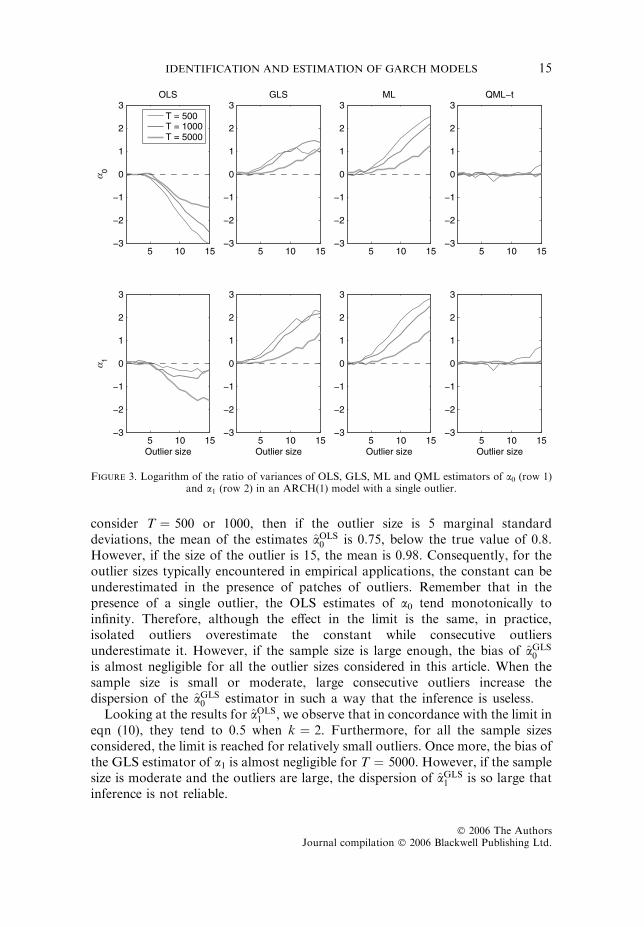
We also analyse how an isolated outlier affects the estimated variances of theOLS and GLS estimators. Figure 3 plots the logarithm of the ratio of the samplevariance of aOLS

0 and aOLS1 in the Monte Carlo experiments, and the estimated

asymptotic variance computed as in eqn (7) and averaged through all MonteCarlo replicates. As we can see in the graph (columns 1 and 2), the asymptoticvariances of the OLS estimator overestimate the sample variances while theasymptotic variances of the GLS estimator underestimate them.



To analyse the effect of consecutive outliers, each simulated series has alsobeen contaminated by two consecutive outliers of the same sizes as above.Figure 4 plots kernel estimates of the densities of the OLS and GLS estimatorsof a0 and a1. It is important to note that although in the limit aOLS

0

increases with x, a0 can be underestimated for small outliers. For example,

0.5 1 1.5 2 0

5

10 = 0

0 S

L

O

T = 500 T = 1000 T = 5000 True parameter

0.5 1 1.5 2 0

5

10 = 5

0.5 1 1.5 2 0

5

10 = 10

0.5 1 1.5 2 0

5

10 = 15

0.5 1 1.5 2 0

5

10 ω =0

0 S

L

G

0.5 1 1.5 2 0

5

10

0.5 1 1.5 2 0

5

10

0.5 1 1.5 2 0

5

10

0.5 1 1.5 2 0

5

10

0 L

M

0.5 1 1.5 2 0

5

10

0.5 1 1.5 2 0

5

10

0.5 1 1.5 2 0

5

10

0.5 1 1.5 2 0

5

10

0 t

−L M

Q

0.5 1 1.5 2 0

5

10

0.5 1 1.5 2 0

5

10

0.5 1 1.5 2 0

5

10

0 0.5 1 0

5

10 = 0

1 S

L

O

0 0.5 1 0

5

10 = 5

0 0.5 1 0

5

10 = 10

0 0.5 1 0

5

10 = 15

0 0.5 1 0

5

10

1 S

L

G

0 0.5 1 0

5

10

0 0.5 1 0

5

10

0 0.5 1 0

5

10

0 0.5 1 0

5

10

1 L

M

0 0.5 1 0

5

10

0 0.5 1 0

5

10

0 0.5 1 0

5

10

0 0.5 10

5

10

1 t

−L M

Q

0 0.5 10

5

10

0 0.5 10

5

10

0 0.5 10

5

10

a

w

w w w w

w w w

a a

a a

a a

a

Figure 2. Kernel estimation of the density of OLS, GLS, ML and QML estimators of a0 (rows 1 to 4)and a1 (rows 5 to 8) in an ARCH(1) model with a single outlier of size x.



consider T ¼ 500 or 1000, then if the outlier size is 5 marginal standarddeviations, the mean of the estimates aOLS

0 is 0.75, below the true value of 0.8.However, if the size of the outlier is 15, the mean is 0.98. Consequently, for theoutlier sizes typically encountered in empirical applications, the constant can beunderestimated in the presence of patches of outliers. Remember that in thepresence of a single outlier, the OLS estimates of a0 tend monotonically toinfinity. Therefore, although the effect in the limit is the same, in practice,isolated outliers overestimate the constant while consecutive outliersunderestimate it. However, if the sample size is large enough, the bias of aGLS

0

is almost negligible for all the outlier sizes considered in this article. When thesample size is small or moderate, large consecutive outliers increase thedispersion of the aGLS

0 estimator in such a way that the inference is useless.Looking at the results for aOLS

1 , we observe that in concordance with the limit ineqn (10), they tend to 0.5 when k ¼ 2. Furthermore, for all the sample sizesconsidered, the limit is reached for relatively small outliers. Once more, the bias ofthe GLS estimator of a1 is almost negligible for T ¼ 5000. However, if the samplesize is moderate and the outliers are large, the dispersion of aGLS

1 is so large thatinference is not reliable.

5 10 15−3

−2

−1

0

1

2

30

OLS

5 10 15−3

−2

−1

0

1

2

3GLS

5 10 15−3

−2

−1

0

1

2

3ML

5 10 15−3

−2

−1

0

1

2

3QML−t

5 10 15−3

−2

−1

0

1

2

3

1

Outlier size5 10 15

−3

−2

−1

0

1

2

3

Outlier size5 10 15

−3

−2

−1

0

1

2

3

Outlier size5 10 15

−3

−2

−1

0

1

2

3

Outlier size

T = 500T = 1000T = 5000

aa

Figure 3. Logarithm of the ratio of variances of OLS, GLS, ML and QML estimators of a0 (row 1)and a1 (row 2) in an ARCH(1) model with a single outlier.



Finally, the logarithm of the ratio of the sample variance and the estimatedasymptotic variance of the OLS and GLS estimators is plotted in Figure 5,where it is shown (see column 1) that, for the OLS estimator of a0 and a1, thisratio tends to zero with the size of the outlier. Therefore, the asymptoticvariance of the OLS estimator, estimated using eqn (7), overestimates the true

0.5 1 1.5 2 0

5

10 = 0

0 S

L

O

0.5 1 1.5 2 0

5

10 = 5

0.5 1 1.5 2 0

5

10 = 10

T = 500T = 1000T = 5000True parameter

0.5 1 1.5 2 0

5

10 = 15

0.5 1 1.5 2 0

5

10 = 0

0 S

L

G

0.5 1 1.5 2 0

5

10

0.5 1 1.5 2 0

5

10

0.5 1 1.5 2 0

5

10

0.5 1 1.5 2 0

5

10

0 L

M

0.5 1 1.5 2 0

5

10

0.5 1 1.5 2 0

5

10

0.5 1 1.5 2 0

5

10

0.5 1 1.5 2 0

5

10

0 t

−L M

Q

0.5 1 1.5 2 0

5

10

0.5 1 1.5 2 0

5

10

0.5 1 1.5 2 0

5

10

0 0.5 1 0

5

10 = 0

1 S

L

O

0 0.5 1 0

5

10 = 5

0 0.5 1 0

5

10 = 10

0 0.5 10

5

10 = 15

0 0.5 1 0

5

10

1 S

L

G

0 0.5 1 0

5

10

0 0.5 1 0

5

10

0 0.5 10

5

10

0 0.5 1 0

5

10

1 L

M

0 0.5 1 0

5

10

0 0.5 1 0

5

10

0 0.5 10

5

10

0 0.5 1 0

5

10

1 t

−L M

Q

0 0.5 1 0

5

10

0 0.5 1 0

5

10

0 0.5 10

5

10

a

w

w

w w w w

w w w

a a

a a

a a

a

Figure 4. Kernel estimation of the density of OLS, GLS, ML and QML estimators of a0 (rows 1 to 4)and a1 (rows 5 to 8) in an ARCH(1) model with two consecutive outliers.



variance, which tends to zero with the size of the outlier. Notice that in thiscase, the biases are larger than in the presence of a single outlier. moreover, theestimated asymptotic variances of the GLS estimator, strongly underestimatethe sample variances for consecutive outliers larger than 5 standard deviations(see column 2).

4.3. Maximum likelihood estimator

Engle (1982) proposed to estimate the parameters of the ARCH(p) model by ML.The distribution of yt conditional on Yt�1 ¼ fyt�1,yt�2, . . . , y1g is Nð0; r2

t Þ andthe log-likelihood function is given by

L ¼ � T � p2

logð2pÞ � 1

2

XT

t¼pþ1log r2

t þy2tr2

t

� �: ð13Þ

If the second-order moment of yt is finite, then,

5 10 15−6

−4

−2

0

2

4

60

OLS

5 10 15−6

−4

−2

0

2

4

6GLS

5 10 15−6

−4

−2

0

2

4

6ML

5 10 15−6

−4

−2

0

2

4

6QML−t

5 10 15−6

−4

−2

0

2

4

6

1

Outlier size5 10 15

−6

−4

−2

0

2

4

6

Outlier size5 10 15

−6

−4

−2

0

2

4

6

Outlier size5 10 15

−6

−4

−2

0

2

4

6

Outlier size

T = 500T = 1000T = 5000

aa

Figure 5. Logarithm of the ratio of variances of OLS, GLS, ML and QML estimators of a0 (row 1)and a1 (row 2) in an ARCH(1) model with two consecutive outliers.



ffiffiffiffiTpðaML � aÞ!d Nð0; ½IðaÞ��1Þ where IðaÞ ¼ E½� @2L

@a@a0�

is the information matrix (see, e.g. Ling and McAleer, 2003).Given that there are no closed-form expressions of the ML estimators of the

parameters a0, a1, . . . , ap, the analysis of the effects of outliers on the MLestimator has been carried out by simulation [see, e.g. Muller and Yohai, 2002,who show that the mean squared error of the ML estimator of the parameters ofARCH(1) models is dramatically influenced by isolated outliers]. On the otherhand, Mendes (2000) shows that the influence functional of the ML estimator ofthe parameters of an ARCH(1) model is the product of a constant vector by aquadratic function of the outlier size. Consider the simplest ARCH(1) model. Inthis case, the log-likelihood function is given by

L ¼ � T � 2

2logð2pÞ � 1

2

XT

t¼2logða0 þ a1y2t�1Þ þ

y2tða0 þ a1y2t�1Þ

� �

which leads to the following ML equations to obtain the estimated parameters

XT

t¼2

y2tr4

t¼XT

t¼2

1

r2tXT

t¼2

y2t�1y2tr4

t¼XT

t¼2

y2t�1r2

t

Multiplying and dividing the right-hand side by r2t ¼ a0 þ a1y2t�1 we obtain

a0XT

t¼2

1

r4tþ a1

XT

t¼2

y2t�1r4

t¼XT

t¼2

y2tr4

t

and

a0XT

t¼2

y2t�1r4

tþ a1

XT

t¼2

y4t�1r4

t¼XT

t¼2

y2t�1y2t

r4t

These two equations represent theML estimator as the result of solving a systemof equations which is the same system solved by the GLS estimator considered inthe previous2 subsection. Therefore, as ML and GLS are asymptotically equivalent,the effects of outliers on both estimators should be similar for large samples.Figure 2 plots the kernel estimates of the densities of theML estimators of a0 and a1when the ARCH(1) series are contaminated by a single outlier of size x. This figureillustrates that when x ¼ 0 the GLS and ML estimators are asymptoticallyequivalent. However, the finite sample distribution of both estimators can be ratherdifferent in the presence of large outliers and moderate sample sizes. Note that, forsample sizes of T ¼ 500 and 1000 and outliers of sizes 10 and 15 standarddeviations, the kernel estimated density of both aML

0 and aML1 are bimodal and non-

symmetric. The bimodality of the ML estimator in the presence of outliers has alsobeen pointed out by Doornik and Ooms (2003). Hence, tests based on normality



will be inadequate. Looking for example at the seventh row of Figure 2, we can seethat in the presence of an outlier of size 15 standard deviations in a sample of sizeT ¼ 500, aML

1 could take any value between 0 and 1, although values close to zeroseem to be more probable, like what we had for aOLS

1 and aGLS1 . Finally, if the

sample size is 5000, the sample distributions of the GLS and ML are similar.Therefore, it is important to point out that the results in Figure 2 suggest that, inmoderate samples, the GLS estimator has certain advantages over the MLestimator in the presence of large isolated outliers. In particular, both estimatorshave similar negative biases but the dispersion of the GLS is smaller.

Figure 3 (column 3) plots the logarithm of the ratio of the sample variance andthe estimated asymptotic variance averaged over all Monte Carlo replicates foraML0 and aML

1 respectively. We can see that this ratio is larger than the ratio of theGLS estimator. Therefore, the asymptotic variance of the ML estimatorunderestimates, in the presence of large isolated outliers, the sample variancemore than the GLS estimator.

The Monte Carlo densities when the series are contaminated by twoconsecutive outliers appear in Figure 4 (rows 3 and 7). As we can see in theplots, the effects caused by two consecutive outliers on the ML estimators are verysimilar to the effects caused by a single outlier. Finally, the effects of consecutiveoutliers on the estimated variances of the ML estimator are weaker than for theGLS estimator (see Figure 5).

4.4. Quasi-Maximum Likelihood estimator

As mentioned in the Introduction, the presence of outliers could be the reason ofthe excess kurtosis found in the standardized observations after an ARCH-typemodel has been fitted to explain the dynamic evolution of second order moments.However, many authors have claimed that this excess kurtosis can be explained bya heavy-tailed conditional distribution; see, for example, Bollerslev (1987), Baillieand Bollerslev (1989), Hsieh (1989), Nelson (1991) and Fiorentini et al. (2003)among many others. Furthermore, Sakata and White (1998) show that QMLestimators based on heavy-tailed distributions are robust in the presence ofoutliers. Consequently, in this subsection, we study the finite sample behavior ofthe QML estimator based on maximizing the Student-likelihood when the data isgenerated by conditionally Gaussian ARCH(1) models contaminated by isolatedand consecutive outliers. If no outliers are present, Newey and Steigerwald (1997)show that when the assumed and true densities are symmetric, the QML estimatoris consistent and efficient.2 The log-likelihood function is given by

LS ¼XT

t¼2log C

gþ 1

2g

� �� log C

1

2g

� �� 1

2log

1� 2gg

� �þ log p

��

þ logða0 þ a1y2t�1Þ þgþ 1

glog 1þ g

1� 2gyt2

ao þ a1y2t�1

� �



where C(�) is the gamma function and g ¼ 1/m, where m are the degrees of freedomof the Student t distribution. The parameter g can be considered as a measure oftail thickness which always remains in the finite range 0 � g < 0.5 if theconditional distribution is restricted to have finite variance, i.e. m > 2 (seeFiorentini et al., 2003).

Rows 4 and 8 of Figure 2 plot the Monte Carlo densities of the QML estimatorof a0 and a1 respectively, when the series are generated by the same ARCH(1)model considered before and contaminated by isolated outliers of size x ¼ 0, 5,10 and 15 marginal standard deviations. This figure shows that when x ¼ 0, thebehaviour of the QML estimator is very similar to ML. However, as postulated bySakata and White (1998), maximizing the Student t likelihood protects againstoutliers even when they are rather large. It can be observed that the QMLestimator is almost unaffected by the presence of outliers. Notice that even insmall sample sizes the biases of aQML�t

0 and aQML�t1 are almost negligible. The

average over the Monte Carlo replicates of the degrees of freedom estimates is83.64 when x ¼ 0 and T ¼ 1000 while it is 9.73 when x ¼ 15. We obtain similarresults for the other sample sizes. With respect to the estimated asymptoticstandard deviations, the last column of Figure 3 shows that they are not affectedby single outliers even if their sizes are large or the sample sizes are small. Thesame conclusions can be obtained from Figures 4 and 5 which plot thecorresponding kernel densities of the QML estimators of a0 and a1 and the log-ratios of their variances obtained when the series are contaminated by twoconsecutive outliers.

5. EFFECTS OF OUTLIERS ON THE ESTIMATION OF GARCH MODELS

In this section we analyse the effects of outliers on three estimators of theparameters of GARCH(1,1) models. First, we analyse the finite sample propertiesof the ML and QML estimators described above for ARCH models. Second, weconsider the closed-form estimator proposed by Kristensen and Linton (2006)which is based on the Yule–Walker equations corresponding to the ARMArepresentation of squared observations.

The robustness properties of the QML3 estimator of the parameters ofGARCH models have been analysed by Sakata and White (1998) and Mendes(2000). The former authors show that when the conditional mean is known, QMLestimators based on thin-tailed distributions as the normal are not robust tooutliers and have a breakdown point equal to zero. On the other hand, QMLestimators obtained by maximizing a log-likelihood function with a fat-taileddistribution are resistant to outliers as long as there are no scale leverage points.Later, Mendes (2000) proves that the QML estimator obtained by maximizing theGaussian log-likelihood has zero breakdown point and unbounded influencecurves. In this article also, some Monte Carlo evidence is presented on the finitesample performance of the QML estimator in the presence of outliers concluding



that the bias and standard errors of the QML estimates increase with thepercentage of contamination and that for very large outliers, they ignore thedynamics in the second moments and act as an inflated scale estimate ofindependent observations. In this section, we generalize and extend thissimulation evidence by carrying out detailed Monte Carlo experiments toanalyse the biases caused by isolated and consecutive LO on the QML estimatorof the parameters of GARCH(1,1) models.

Figure 6 contains the kernel estimates of the density of a0, a1, b and a1 þ b forML and QML estimates based on 1000 replicates, for a GARCH(1,1) model withparameters a0 ¼ 0.1, a1 ¼ 0.1 and b ¼ 0.8, contaminated with a single outlier ofsizes x ¼ 0, 5, 10 and 15 standard deviations. This figure shows that, unless thesample size is very large, like T ¼ 5000, ML estimators as expected are notrobust to the presence of outliers. The same conclusion is obtained by Mendes(2000) and Sakata and White (1998). The QML estimator has an interestingbehaviour. It is robust for a1, as in the case of ARCH models, but not for a0, band a1 þ b. Note that the Student t-tails are robust for isolated outliers in ARCHmodels but for GARCH models one isolated outlier at time t affects theestimation of the conditional variance at time t þ 1, and this variance will be usedin the estimation of the conditional variance at time t þ 2. Thus, an isolatedoutlier behaves as a patch of outliers for the estimation of the conditionalvariance. This explains the different behaviour of the QML estimator for ARCHand GARCH models.

In our Monte Carlo experiments we have also observed that although thegenerating model has finite fourth-order moment, the presence of outliers leads toa large proportion of ML estimates which do not satisfy the correspondingcondition. For example, when T ¼ 500 and x ¼ 15, 36% of the ML estimates ofa1 and b do not satisfy it. In our simulations, we often observed replicates forwhich the estimated ML asymptotic covariance matrix is nearly singular. Thiscould be due to the estimates aML

1 and bML taking values close to zero and onerespectively, and the determinant of the information matrix being very close tozero. Sakata and White (1998) also observe in real data that, as a consequence ofextreme outliers, the usual plug-in asymptotic covariance matrix could be nearlysingular. Consequently, we do not report the results on the ratio of the samplevariance and the estimated asymptotic variance although we have observed that,when the latter variances are defined, their behaviour is similar to the oneobserved for the ML estimator in Figures 3 and 5. Therefore, when using theestimated asymptotic ML covariance matrix we may have a false security on theinference on the GARCH parameters. The usual hypothesis testing methods willbe highly unreliable.

Figure 7 plots kernel estimates of the density of the parameters for the sameGARCH(1,1) model but now contaminated with two consecutive outliers. Thisfigure shows that aML

0 and aML1 overestimate the true parameters, and bML is

underestimating the true b. Note that if the outliers are large and the sample size ismoderate, the sample densities of aML

1 and bML are such that standard inference isnot reliable. Furthermore, this figure shows that large consecutive outliers can



have dramatic effects on the estimated persistence. For example, when x ¼ 15and T ¼ 500 or 1000, the estimated density of aML

1 þ bML has two modes, onearound zero and the other close to one. The estimates of the persistence are onlyreliable for very large sample sizes. The biases caused by consecutive outliers on

0 1 2 0

5

10

0 L

M

= 0

T = 500 T = 1000 T = 5000 True parameter

0 1 2 0

5

10 = 5

0 1 2 0

5

10 = 10

0 1 2 0

5

10 = 15

0 0.5 1 0

5

10

1 L

M

0 0.5 1 0

5

10

0 0.5 1 0

5

10

0 0.5 1 0

5

10

0 0.5 1 0

5

10

L M

0 0.5 1 0

5

10

0 0.5 1 0

5

10

0 0.5 1 0

5

10

0 0.5 1 0

5

10

1L

M +

L

M

0 0.5 1 0

5

10

0 0.5 1 0

5

10

0 0.5 1 0

5

10

0 1 2 0

5

10

0 t

−L M

Q

= 0

0 1 2 0

5

10 = 5

0 1 2 0

5

10 = 10

0 1 20

5

10 = 15

0 0.5 1 0

5

10

1 t

−L M

Q

0 0.5 1 0

5

10

0 0.5 1 0

5

10

0 0.5 10

5

10

0 0.5 1 0

5

10

t −L

M

Q

0 0.5 1 0

5

10

0 0.5 1 0

5

10

0 0.5 10

5

10

0 0.5 1 0

5

10

1 t

−L M

Q

+

t

−L M

Q

0 0.5 1 0

5

10

0 0.5 1 0

5

10

0 0.5 10

5

10

a a

b a

w w w w

w w w w

a b

b a

b a

Figure 6. Kernel estimation of the density of ML and QML estimators of a0 (rows 1 and 5), a1 (rows 2and 6), b (rows 3 and 7) and a1 þ b (rows 4 and 8) in a GARCH(1,1) model with a single outlier.



the estimated asymptotic covariance matrix of the ML estimators are similar tothose caused by a single outlier. Regarding the QML estimator, as before, it isrobust for a1 but not for a0, b and a1 þ b.

Finally, it is interesting to analyse the effects of outliers on the closed-formestimator for GARCH(1,1) models proposed by Kristensen and Linton (2006).

0 1 2 0

5

10

0 ML

= 0

T = 500T = 1000T = 5000True parameter

0 1 2 0

5

10 = 5

0 1 2 0

5

10 = 10

0 1 2 0

5

10 = 15

0 0.5 1 0

5

10

1 ML

0 0.5 1 0

5

10

0 0.5 1 0

5

10

0 0.5 1 0

5

10

0 0.5 1 0

5

10

ML

0 0.5 1 0

5

10

0 0.5 1 0

5

10

0 0.5 1 0

5

10

0 0.5 1 0

5

10

1 ML +

ML

0 0.5 1 0

5

10

0 0.5 1 0

5

10

0 0.5 1 0

5

10

0 1 2 0

5

10

0 QM

L−t

= 0

0 1 2 0

5

10 = 5

0 1 2 0

5

10 = 10

0 1 20

5

10 = 15

0 0.5 1 0

5

10

1 QM

L−t

0 0.5 1 0

5

10

0 0.5 1 0

5

10

0 0.5 10

5

10

0 0.5 1 0

5

10

QM

L−t

0 0.5 1 0

5

10

0 0.5 1 0

5

10

0 0.5 10

5

10

0 0.5 1 0

5

10

QM

L−t +

QM

L−t

0 0.5 1 0

5

10

0 0.5 1 0

5

10

0 0.5 10

5

10

a

w

w w w w

w w w

a b

a a

a b

b a

b

Figure 7. Kernel estimation of the density of ML and QML estimators of a0 (rows 1 and 5), a1 (rows 2and 6), b (rows 3 and 7) and a1 þ b (rows 4 and 8) in a GARCH(1,1) model with two consecutive

outliers.



Assuming yt ¼ etrt where r2t ¼ a0 þ a1y2t�1 þ br2

t�1 we also have theARMA(1,1) representation for the squared observations given by y2t ¼a0 þ /y2t�1 þ mt � bvt�1, where / ¼ a1 þ b and the noise, mt ¼ r2

t ðe2t � 1Þ, is azero-mean heteroscedastic uncorrelated sequence. Calling r(h) as before theautocorrelation of the squared observations and using the relationship betweenthese autocorrelations and the ARMA parameters, Kristensen and Linton (2006)propose the estimates

/ ¼Xk

j¼2

wjrðjÞrðj� 1Þ

where wj is a weighting function and

b ¼ ðb�ffiffiffiffiffiffiffiffiffiffiffiffiffib2 � 4p

Þ2

with b ¼ ð/2 þ 1� 2 /rð1ÞÞð/� rð1ÞÞ

and a1 ¼ /� b:

In their simulation study, the weights are chosen as wj ¼ 1/3 for j ¼ 1,2,3 andwj ¼ 0 for j > 3. Although, as shown by these authors, this estimate seems towork well without outliers, the effect of contamination in this estimate can bevery large. We have seen that a single large outlier will make all the coefficientsr(j) small and thus the estimate /, computed as a ratio of small numbers, willhave a large variance and it may be unreliable. Note that the estimate /obtained does not need to be small. For patches of outliers, the coefficients r(j)will be large and of similar size and the estimate / will be close to one and willnot suffer for the large variability. However, the equation for b will not bereliable anymore, because of the large bias of the autocorrelation coefficientsand b is often found to be smaller than 2. As this parameter is constrained to beb > 2 the censoring leads to b ¼ 2 þ e and then the estimate of b will be closeto one and a1 will be forced to be close to zero. This result has been checked byMonte Carlo.

6. CONCLUSIONS

Our results can be important in several directions. First of all, a lot of care shouldbe taken when assuming conditional heteroscedasticity from a correlogram ofsquares with a large first-order autocorrelation followed by small coefficients forhigher lags. We have seen that this pattern could be caused by two largeconsecutive outliers, regardless of whether the data-generating process ishomoscedastic or heteroscedastic. Therefore, if the uncontaminated process ishomoscedastic, after cleaning the outliers we will expect that the order-oneautocorrelation will not be significant anymore. On the other hand, if theuncontaminated series is heteroscedastic, after correcting for outliers we expectthat the first-order autocorrelation coefficient will decrease, while all the othercoefficients will increase and become significant. Second, before rejecting the



presence of conditional heteroscedasticity we should check that the series does nothave large isolated outliers, as they bias all the autocorrelations towards zero.

Third, outliers may have a strong effect on the size and power of popular testsof conditional homoscedasticity based on autocorrelations of squares. On the onehand, a very large isolated outlier leads to tests which never reject the nullhypothesis of homoscedasticity, regardless of whether the uncontaminated seriesis homoscedastic or heteroscedastic. On the other hand, two or more largeconsecutive outliers lead to tests which always reject the null hypothesis ofhomoscedasticity, even if the uncontaminated series is truly homoscedastic. Notethat in the empirical analysis of financial returns it is more likely to findconsecutive outliers because the series of returns is obtained as differences of thelogarithmic prices. If the prices have a permanent shock, then the returns willshow an isolated outlier but if the prices have a transitory movement during justone period of time, the returns will show two consecutive outliers. Therefore, careshould be taken when the null of homoscedasticity is rejected especially if only thefirst-order autocorrelation is significantly different from zero.

Fourth, in moderately large samples, the QML estimator of ARCH modelsbased on the Student likelihood, is more robust than the OLS, GLS and MLestimators in the presence of additive outliers. This QML estimator is robustagainst outliers without losing the good properties of ML for uncontaminatedseries. The OLS estimator has larger biases and the inference based on theestimated standard deviations is not reliable because they overestimate the truedispersion of the estimator. Furthermore, the negative estimates of the ARCHparameters that are sometimes obtained in empirical applications could be due tooutliers. The sample distribution of the ML estimator of the ARCH parameterscan be bimodal in the presence of outliers, implying important problems forinference.

Fifth, for GARCH (1,1) models the ML estimator of the parameters has verylarge dispersion even in moderately large samples as T ¼ 1000, and the samehappens for the GLS estimator. The QML estimator based on the Studentlikelihood is more robust than GLS and ML, but fails to be robust in general,especially for the estimation of the b parameter.

Thus, when fitting GARCH-type models to conditionally heteroscedastic seriesit is always advisable to check if the series is affected by outliers. There are severalprocedures proposed in the literature to test for outliers in the presence ofGARCH effects and the comparison of these procedures will be the subject offurther research.

ACKNOWLEDGEMENTS

Financial support from projects SEJ2004-03303, BEC2002.03720 and SEJ2005-02829/ECON by the Spanish Government and from Instituto Valenciano de



Investigaciones Econ�omicas (IVIE) is gratefully acknowledged. We are alsograteful to the comments of two anonymous referees that have helped us toimprove this article. Any remaining errors are our own.

NOTES

1. Although the LM and Q(m) tests are asymptotically equivalent, they testdifferent null hypotheses. The null hypothesies of the LM test is that theparameters of an ARCH(p) model associated with lagged squared observationsare equal to zero while the McLeod–Li test is model-free in the sense that thenull hypothesis is that the first m autocorrelations are jointly equal to zero.

2. When this symmetry condition is not satisfied, Newey and Steigerwald (1997)show that, unless the conditional mean is identical to zero, the QML estimatoris consistent if an additional location parameter is added to the model. Giventhat outliers can generate asymmetries, we also consider the introduction ofthis additional parameter. The modified ARCH(p) model is given by yt ¼(d þ et)rt where

r2t ¼ a0 þ

Xp

i¼1aiy2t�i:

The results are the same as those obtained when d ¼ 0 and, consequently, theyare not reported.

3. Note that in this article, the QML estimator refers to the estimator thatmaximizes the Student likelihood when the conditional distribution is notStudent. However, the QML estimator is obtained when maximizing alikelihood that is not the same as the conditional distribution of the series. Infact, the most popular use of the QML estimator is when maximizing theGaussian likelihood when the errors are not Gaussian.

Corresponding author; Esther Ruiz, Dpt. Estadıstica, Universidad Carlos III deMadrid, C/ Madrid 126, 28903 Getafe, Spain. Tel.: 34 91 6249851; Fax: 34 916249849; E-mail: [email protected]

REFERENCES

Aggarwal, R., Inclan, C. and Leal, R. (1999) Volatility in emerging stock markets. Journal ofFinancial and Quantitative Analysis 34, 33–5.

Baillie, R. and Bollerslev, T. (1989) The message in daily exchange rates: a conditional-variancetale. Journal of Business & Economic Statistics 7, 297–305.

Balke, N. S. and Fomby, T. B. (1994) Large shocks, small shocks and economic fluctuations: outliersin macroeconomic time series. Journal of Applied Econometrics 9, 181–200.



Bollerslev, T. (1986) Generalized autoregressive conditional heteroskedasticity. Journal of Econo-metrics 31, 307–27.

Bollerslev, T. (1987) A conditionally heteroskedastic time series model for speculative prices andrates of return. The Review of Economics and Statistics 69, 542–7.

Bollerslev,3 T, Engle, R.F. and Nelson, D.B. (1994) ARCH models. In Handbook of Econometrics,Vol. 4 (eds R. F. Engle and D. L. McFadden). New York: Elsevier Science.

Bose, A. and Mukherjee, K. (2003) Estimating the ARCH parameters by solving linear equations.Journal of Time Series Analysis 24, 127–36.

Carnero, M. A (2003) Heterocedasticidad condicional, Atıpicos y Cambios de nivel en seriestemporales financieras. Ph.D. Thesis, Universidad Carlos III de Madrid.

Doornik, J. A. and Ooms, M. (2003) Multimodality in the GARCH regression model. Manuscript,Nuffield College, University of Oxford.

Engle, R. F. (1982) Autoregressive conditional heteroskedasticity with estimates of the variance ofUnited Kingdom inflation. Econometrica 50, 987–1007.

Fiorentini, G., Sentana, E. and Calzolari, G. (2003) Maximum likelihood estimation and inferencein multivariate conditionally heteroscedastic dynamic regression models with Student t innovations.Journal of Business & Economic Statistics 21, 532–46.

Franses, P. H. and Ghijsels, E. (1999) Additive outliers, GARCH and forecasting volatility.International Journal of Forecasting 15, 1–9.

Franses, P. H., Van Dijk, D. and Lucas, A. (2004) Short patches of outliers, ARCH and volatilitymodelling. Applied Financial Economics 14, 221–31.

Hsieh, D. (1989) Modelling heteroscedasticity in daily foreign-exchange rates. Journal of Business &Economic Statistics 7, 307–17.

Hotta, L. K. and Tsay, R. S. (1998) Outliers in GARCH processes.4 Manuscript.Kristensen, D. and Linton, O. (2006) A closed-form estimator for the GARCH(1,1)-model.

Econometric Theory 22, 323–37.Lee, J. H. H. and King, M. L. (1993) A locally most mean powerful based score test for ARCH and

GARCH regression disturbances. Journal of Business and Economic Statistics 11, 17–27.Li, J. and Kao, C. (2002) A bounded influence estimation and outlier detection for ARCG/GARCH

models with an application to foreign exchange rates. Manuscript.Ling, S. and McAleer, M. (2003) Asymptotic theory for a vector ARMA-GARCH model.

Econometric Theory 19, 280–310.McLeod, A. J. and Li, W. K. (1983) Diagnostic checking ARMA time series models using squared-

residual correlations. Journal of Time Series Analysis 4, 269–73.Mendes, B. V. M. (2000) Assessing the bias of maximum likelihood estimates of contaminated

GARCH models. Journal of Statistical Computation and Simulation 67, 359–76.Muller, N. and Yohai, V. J. (2002) Robust estimates for ARCH processes. Journal of Time Series

Analysis 23, 341–75.Nelson, D. (1991) Conditional heteroskedasticity in asset returns: a new approach. Econometrica 59,

347–70.Newey, W. K. and Steigerwald, D. G. (1997) Asymptotic bias for quasi-maximum-likelihood

estimators in conditional heteroskedasticity models. Econometrica 65, 587–99.Pena, D. (2001) Outliers, influential observations and missing data. In A Course in Time Series (eds

D. Pena, G. C. Tiao and R. S. Tsay). Wiley.5Pena, D. and Rodriguez, J. (2002) A powerful portmanteau test of lack of fit in time series. Journal of

the American Statistical Association 97, 601–10.Rodriguez, J. and Ruiz, E. (2005) A powerful test for conditional heteroscedasticity for financial time

series with highly persistent volatilites. Statistica Sinica 15, 505–25.Sakata, S. and White, H. (1998) High breakdown point conditional dispersion estimation with

application to S&P500 daily returns volatility. Econometrica 66, 529–67.Van Dijk, D., Franses, P. H. and Lucas, A. (1999) Testing for ARCH in the presence of additive

outliers. Journal of Applied Econometrics 14, 539–62.Weiss, A. (1986) Asymptotic theory for ARCH models. Econometric Theory 2, 107–31.Wooldridge, J. M. (1990) A unified approach to robust regression based specification tests.

Econometric Theory 6, 17–43.



Author Query Form

Journal: JTSA

Article: 519

Dear Author,During the copy-editing of your paper, the following queries arose. Pleaserespond to these by marking up your proofs with the necessary changes/addi-tions. Please write your answers on the query sheet if there is insufficient spaceon the page proofs. Please write clearly and follow the conventions shown onthe attached corrections sheet. If returning the proof by fax do not write tooclose to the paper’s edge. Please remember that illegible mark-ups may delaypublication.

Many thanks for your assistance.

Query

reference

Query Remarks

Q1 AU: Production Editor: Please provide date of

receipt of the first version of the manuscript

Q2 AU: please indicate the exact Subsection instead

of ‘Previous Subsection�

Q3 AU: Please provide page range

Q4 AU: Please provide the name of the institute/

univesity where the manuscript is present in

Hotta and Tsay (1998) and Li and Kao (2002)

Q5 AU: Please provide location (city) of publisher

and page range of chapter in Pena (2001)

Effects of outliers on the identification and estimation of GARCH models

Documents

Transcript of Effects of outliers on the identification and estimation of GARCH models