Published in Image Processing On Line on 2012–05–19.ISSN 2105–1232 c© 2012 IPOL & the authors CC–BY–NC–SAThis article is available online with supplementary materials,software, datasets and online demo athttp://dx.doi.org/10.5201/ipol.2012.mmm-oh

Automatic Homographic Registration of a Pair of Images,

with A Contrario Elimination of Outliers

Lionel Moisan1, Pierre Moulon2, Pascal Monasse3

1 MAP5, Universite Paris Descartes (lionel.moisan@parisdescartes.fr)2 IMAGINE/LIGM, Universite Paris Est & Mikros Image (pmo@mikrosimage.eu)

3 IMAGINE/LIGM, Universite Paris Est (monasse@imagine.enpc.fr)

Abstract

The RANSAC [2] algorithm (RANdom SAmple Consensus) is a robust method to estimateparameters of a model fitting the data, in presence of outliers among the data. Its randomnature is due only to complexity considerations. It iteratively extracts a random sample out ofall data, of minimal size sufficient to estimate the parameters. At each such trial, the numberof inliers (data that fits the model within an acceptable error threshold) is counted. In the end,the set of parameters maximizing the number of inliers is accepted.

The variant proposed by Moisan and Stival [7] consists in introducing an a contrario [1] criterionto avoid the hard thresholds for inlier/outlier discrimination. It has three consequences:

1. The threshold for inlier/outlier discrimination is adaptive, it does not need to be fixed.

2. It gives a decision on the adequacy of the final model: it does not provide a wrong set ofparameters if it does not have enough confidence.

3. The procedure to draw a new sample can be amended as soon as one set of parameters isdeemed meaningful: the new sample can be drawn among the inliers of this model.

In this particular instantiation, we apply it to the estimation of the homography registering twoimages of the same scene. The homography is an 8-parameter model arising in two situationswhen using a pinhole camera: the scene is planar (a painting, a facade, etc.) or the viewpointlocation is fixed (pure rotation around the optical center). When the homography is found, itis used to stitch the images in the coordinate frame of the second image and build a panorama.The point correspondences between images are computed by the SIFT [5] algorithm.

Source Code

The source code to reproduce the same results as the demo can be found on the article webpage (http://dx.doi.org/10.5201/ipol.2012.mmm-oh). Notice that due to the random com-ponent of ORSA, different runs may yield slightly different results. You may also observe slowerruns on your machine for large images, as the mosaic construction parts use the multiple coresvia OpenMP (http://openmp.org/), and the IPOL server has probably more cores (32 cur-rently).

Supplementary Material

A first implementation by Moisan and Stival of the method as a Megawave2 (http://megawave.cmla.ens-cachan.fr/) module, called stereomatch.c, can be found in [7].

Possible updates, bug fixes, or enhanced versions of the code can be found at http://imagine.enpc.fr/~moulonp/AC_Ransac.html. Notice however that such versions are not necessarilypeer-reviewed.

1

Disclaimer

The present work publishes only the ORSA [7] algorithm as described below (applied to homographyestimation). It does not publish the SIFT subroutine which is called by the demo code. SIFT maybe updated or replaced by other subroutines.

1 Background

1.1 RANSAC

The RANSAC algorithm is used to estimate parameters of a model fitting some data among whichoutliers are present, that is part of the data is corrupted. The assumption is that correct data isconsensual, while incorrect data is random. Let us note Nsample the number of data samples necessaryto estimate the parameters and n the total number of data samples.

1. Randomly draw Nsample random data samples.

2. Estimate parameters Param of the model from these samples.

3. Count number c of inliers among the n data samples given Param, using a threshold σ on theresidual error.

4. If c is larger than its greatest value up to now, store Param and c.

5. Go to step 1 if the allocated number of iterations nIter is not reached.

In point 3 above, distinction between inlier and outlier is done using the parameter σ, a thresholdon the deviation to the model (the “residual error” in regression). Observe that ideally all sets ofNsample data samples should be tested, but this would be too long for even moderate n, except maybewhen Nsample = 2. Hence the random selection in step 1.

As above, we note Nsample the minimal number of data terms to determine a geometric configu-ration with no remaining degree of freedom. For example:

• Nsample = 1 for a translation since one correspondence term determines it.

• Nsample = 2 for a similarity.

• Nsample = 3 for an affine transform.

• Nsample = 4 for a homography.

• Nsample = 7 for a fundamental matrix.

Of course, in all but the first of these cases, there are degenerate situations that do not permita unique estimation. The case of fundamental matrix with the 7-point method is interesting in thatit can yield up to 3 solutions. We will note Noutcomes the number of possible models estimated byNsample data terms. In most cases, Noutcomes = 1.

Line detection example: consider the problem of fitting a line to n 2-D points corrupted by noiseand outliers. In such a case, two points are required to estimate the parameters of a line (Nsample = 2).A point would be deemed inlier if its distance to the line is less than σ. Notice that at the end theresulting line is still estimated from only two points, so may not be very precise. Nevertheless at thispoint we can discard all outliers and compute the regression line of inliers. It is a common procedureto estimate more precisely the model considering only inliers in the end.

2

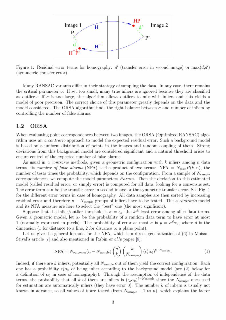
Image 1 Image 2d’

d

H

H−1

PP’

−1

HP

H P’

Figure 1: Residual error terms for homography: d′ (transfer error in second image) or max(d,d′)(symmetric transfer error)

Many RANSAC variants differ in their strategy of sampling the data. In any case, there remainsthe critical parameter σ. If set too small, many true inliers are ignored because they are classifiedas outliers. If σ is too large, the algorithm allows outliers to mix with inliers and this yields amodel of poor precision. The correct choice of this parameter greatly depends on the data and themodel considered. The ORSA algorithm finds the right balance between σ and number of inliers bycontrolling the number of false alarms.

1.2 ORSA

When evaluating point correspondences between two images, the ORSA (Optimized RANSAC) algo-rithm uses an a contrario approach to model the expected residual error. Such a background modelis based on a uniform distribution of points in the images and random coupling of them. Strongdeviations from this background model are considered significant and a natural threshold arises toensure control of the expected number of false alarms.

As usual in a contrario methods, given a geometric configuration with k inliers among n dataterms, its number of false alarms (NFA) is the product of two terms: NFA = NtestsP (k, n), thenumber of tests times the probability, which depends on the configuration. From a sample of Nsample

correspondences, we compute the model parameters Param. Then the deviation to this estimatedmodel (called residual error, or simply error) is computed for all data, looking for a consensus set.The error term can be the transfer error in second image or the symmetric transfer error. See Fig. 1for the different error terms in case of homography. All data samples are then sorted by increasingresidual error and therefore n − Nsample groups of inliers have to be tested. The a contrario modeland its NFA measure are here to select the “best” one (the most significant).

Suppose that the inlier/outlier threshold is σ = εk, the kth least error among all n data terms.Given a geometric model, let α0 be the probability of a random data term to have error at most1 (normally expressed in pixels). The probability of error at most σ is p = σdα0, where d is thedimension (1 for distance to a line, 2 for distance to a plane point).

Let us give the general formula for the NFA, which is a direct generalization of (6) in Moisan-Stival’s article [7] and also mentioned in Rabin et al.’s paper [8]:

NFA = Noutcomes(n−Nsample)

(nk

)(k

Nsample

)(εdkα0)

k−Nsample . (1)

Indeed, if there are k inliers, potentially all Nsample out of them yield the correct configuration. Eachone has a probability εdkα0 of being inlier according to the background model (see (2) below fora definition of α0 in case of homography). Through the assumption of independence of the dataterms, the probability that all k of them are inliers is (εkα0)

k−Nsample since the Nsample ones usedfor estimation are automatically inliers (they have error 0). The number k of inliers is usually notknown in advance, so all values of k are tested (from Nsample + 1 to n), which explains the factor

3

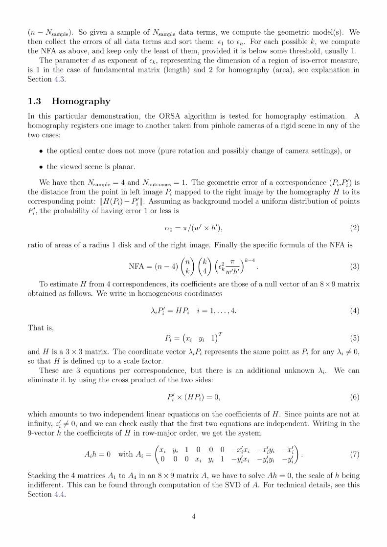
(n − Nsample). So given a sample of Nsample data terms, we compute the geometric model(s). Wethen collect the errors of all data terms and sort them: ε1 to εn. For each possible k, we computethe NFA as above, and keep only the least of them, provided it is below some threshold, usually 1.

The parameter d as exponent of εk, representing the dimension of a region of iso-error measure,is 1 in the case of fundamental matrix (length) and 2 for homography (area), see explanation inSection 4.3.

1.3 Homography

In this particular demonstration, the ORSA algorithm is tested for homography estimation. Ahomography registers one image to another taken from pinhole cameras of a rigid scene in any of thetwo cases:

• the optical center does not move (pure rotation and possibly change of camera settings), or

• the viewed scene is planar.

We have then Nsample = 4 and Noutcomes = 1. The geometric error of a correspondence (Pi,P′i ) is

the distance from the point in left image Pi mapped to the right image by the homography H to itscorresponding point: ‖H(Pi)−P ′i‖. Assuming as background model a uniform distribution of pointsP ′i , the probability of having error 1 or less is

α0 = π/(w′ × h′), (2)

ratio of areas of a radius 1 disk and of the right image. Finally the specific formula of the NFA is

NFA = (n− 4)

(nk

)(k4

)(ε2k

π

w′h′

)k−4. (3)

To estimate H from 4 correspondences, its coefficients are those of a null vector of an 8×9 matrixobtained as follows. We write in homogeneous coordinates

λiP′i = HPi i = 1, . . . , 4. (4)

That is,

Pi =(xi yi 1

)T(5)

and H is a 3× 3 matrix. The coordinate vector λiPi represents the same point as Pi for any λi 6= 0,so that H is defined up to a scale factor.

These are 3 equations per correspondence, but there is an additional unknown λi. We caneliminate it by using the cross product of the two sides:

P ′i × (HPi) = 0, (6)

which amounts to two independent linear equations on the coefficients of H. Since points are not atinfinity, z′i 6= 0, and we can check easily that the first two equations are independent. Writing in the9-vector h the coefficients of H in row-major order, we get the system

Aih = 0 with Ai =

(xi yi 1 0 0 0 −x′ixi −x′iyi −x′i0 0 0 xi yi 1 −y′ixi −y′iyi −y′i

). (7)

Stacking the 4 matrices A1 to A4 in an 8× 9 matrix A, we have to solve Ah = 0, the scale of h beingindifferent. This can be found through computation of the SVD of A. For technical details, see thisSection 4.4.

4

2 Online Demo

The first time you run the demo on a pair of images, the ORSA algorithm determines automaticallythe error threshold, which we call precision. In some cases, it can be useful to set manually amaximum error (for example 1 pixel). This can be done through a drop-down menu in the resultspage. In that situation, the ORSA algorithm still determines automatically the precision, but it isguaranteed to be below the precision set by the user.

The demo offers the possibility to select a rectangle of the first image and try to register only thatpart. In that case, the SIFT points are computed on the full image but those outside the selectionare discarded. Notice that this is not quite the same as applying the SIFT algorithm on the croppedimage because of border effects.

The demo uses the symmetric transfer error (see Figure 1), but the code itself has the possibilityto use the transfer error in second image.

You can regulate the number of correspondences by modifying the SIFT ratio s. The defaultvalue is s = 0.6, which should have very few false positives. Given a SIFT point P of descriptordesc(P ) in image 1, we match it with Q in image 2 if

Q = arg minP ′

d(desc(P ), desc(P ′)) and d(desc(P ), desc(Q)) < s× minP ′ 6=Q

d(desc(P ), desc(P ′)). (8)

In other words, P matches the SIFT point of image 2 of closest descriptor, but only if second closestdescriptor is at s times this descriptor distance. When s = 1, the latter condition is always satisfiedand all SIFT points in image 1 match with one point in image 2. The number of outliers becomeslarge with such a high value, typically 60-70%. To challenge the algorithm even further and havemore outliers, we generalize this condition to the following one when s ≥ 1:

d(desc(P ), desc(Q)) < s×minP ′

d(desc(P ), desc(P ′)). (9)

The point P can now match with several points Q in right image. This is a way to add artificiallyoutliers. In our tests on typical examples, we get around 90% outliers for s = 1.1.

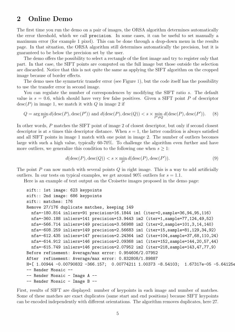
Here is an example of text output on the Croisette images proposed in the demo page:

sift:: 1st image: 623 keypoints

sift:: 2nd image: 686 keypoints

sift:: matches: 176

Remove 27/176 duplicate matches, keeping 149

nfa=-180.814 inliers=91 precision=16.1844 im1 (iter=0,sample=36,94,95,116)

nfa=-360.188 inliers=141 precision=13.9443 im2 (iter=1,sample=77,124,49,52)

nfa=-566.714 inliers=149 precision=3.56988 im2 (iter=2,sample=101,3,14,140)

nfa=-608.259 inliers=149 precision=2.56683 im1 (iter=15,sample=81,129,34,92)

nfa=-612.435 inliers=147 precision=2.24364 im2 (iter=104,sample=37,68,110,24)

nfa=-614.912 inliers=146 precision=2.09368 im1 (iter=152,sample=144,20,57,44)

nfa=-615.749 inliers=146 precision=2.07952 im2 (iter=218,sample=143,47,77,9)

Before refinement: Average/max error: 0.954606/2.07952

After refinement: Average/max error: 0.832808/1.89887

H=[ 1.00944 -0.00790832 -366.157; 0.00774211 1.00373 -8.54103; 1.67317e-05 -5.64125e-06 1 ]

-- Render Mosaic --

-- Render Mosaic - Image A --

-- Render Mosaic - Image B --

First, results of SIFT are displayed: number of keypoints in each image and number of matches.Some of these matches are exact duplicates (same start and end positions) because SIFT keypointscan be encoded independently with different orientations. The algorithm removes duplicates, here 27.

5

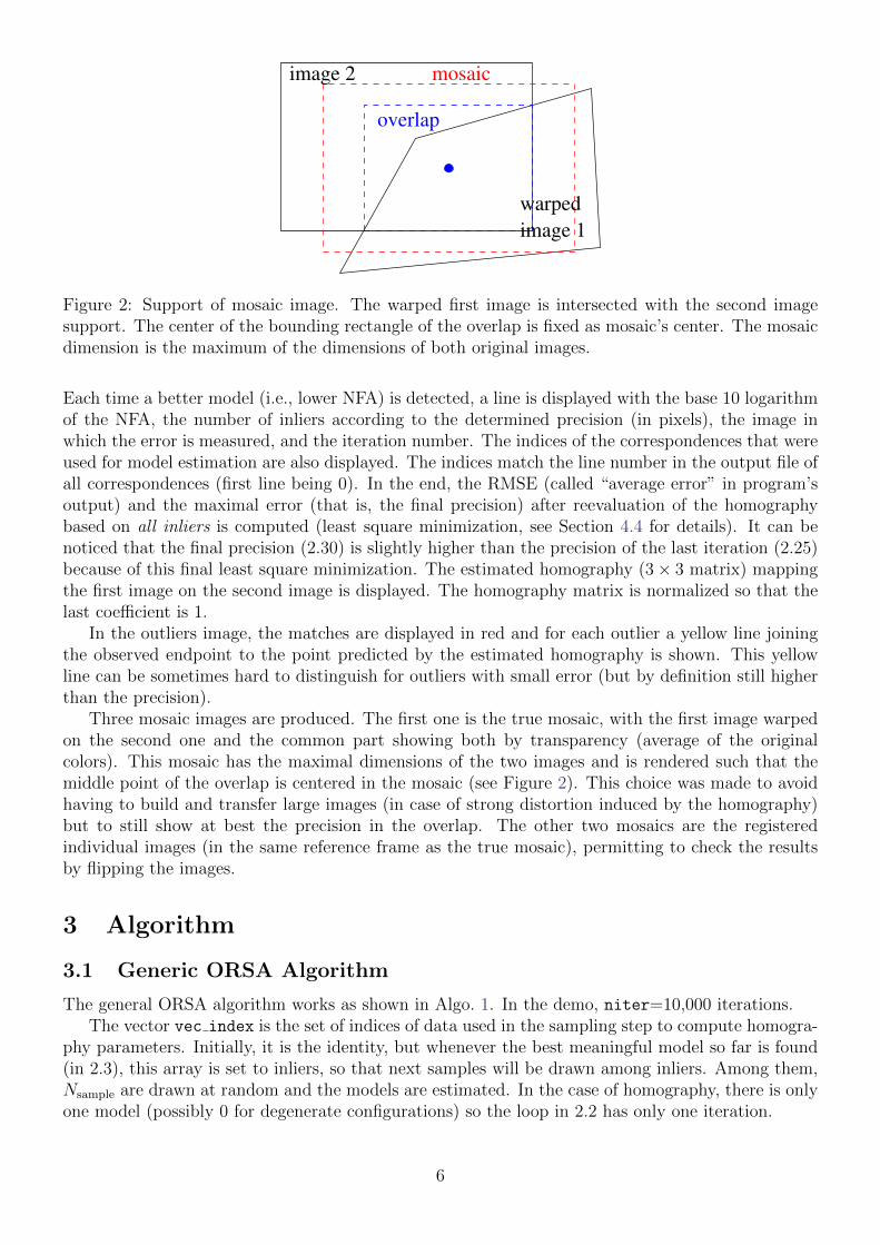
image 2 mosaic

overlap

image 1

warped

Figure 2: Support of mosaic image. The warped first image is intersected with the second imagesupport. The center of the bounding rectangle of the overlap is fixed as mosaic’s center. The mosaicdimension is the maximum of the dimensions of both original images.

Each time a better model (i.e., lower NFA) is detected, a line is displayed with the base 10 logarithmof the NFA, the number of inliers according to the determined precision (in pixels), the image inwhich the error is measured, and the iteration number. The indices of the correspondences that wereused for model estimation are also displayed. The indices match the line number in the output file ofall correspondences (first line being 0). In the end, the RMSE (called “average error” in program’soutput) and the maximal error (that is, the final precision) after reevaluation of the homographybased on all inliers is computed (least square minimization, see Section 4.4 for details). It can benoticed that the final precision (2.30) is slightly higher than the precision of the last iteration (2.25)because of this final least square minimization. The estimated homography (3× 3 matrix) mappingthe first image on the second image is displayed. The homography matrix is normalized so that thelast coefficient is 1.

In the outliers image, the matches are displayed in red and for each outlier a yellow line joiningthe observed endpoint to the point predicted by the estimated homography is shown. This yellowline can be sometimes hard to distinguish for outliers with small error (but by definition still higherthan the precision).

Three mosaic images are produced. The first one is the true mosaic, with the first image warpedon the second one and the common part showing both by transparency (average of the originalcolors). This mosaic has the maximal dimensions of the two images and is rendered such that themiddle point of the overlap is centered in the mosaic (see Figure 2). This choice was made to avoidhaving to build and transfer large images (in case of strong distortion induced by the homography)but to still show at best the precision in the overlap. The other two mosaics are the registeredindividual images (in the same reference frame as the true mosaic), permitting to check the resultsby flipping the images.

3 Algorithm

3.1 Generic ORSA Algorithm

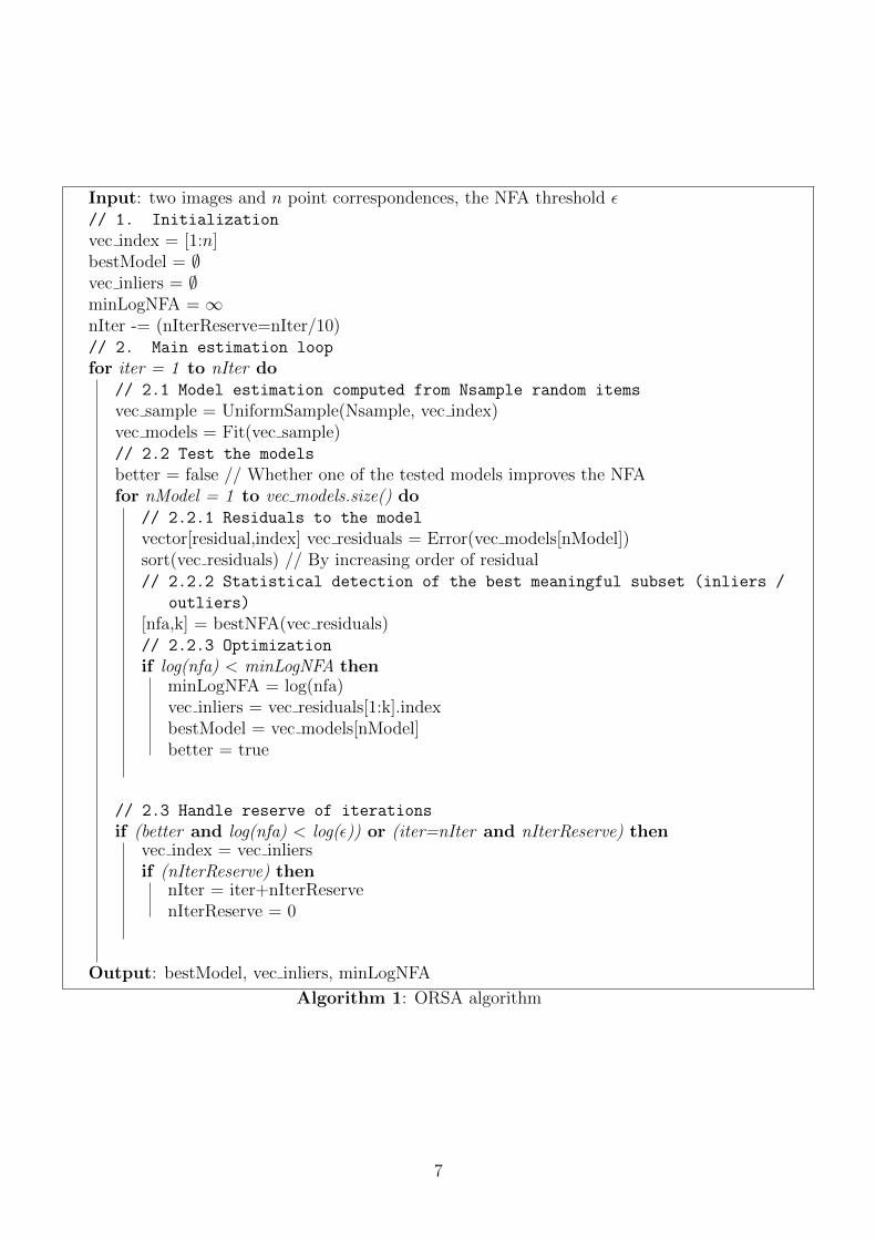
The general ORSA algorithm works as shown in Algo. 1. In the demo, niter=10,000 iterations.The vector vec index is the set of indices of data used in the sampling step to compute homogra-

phy parameters. Initially, it is the identity, but whenever the best meaningful model so far is found(in 2.3), this array is set to inliers, so that next samples will be drawn among inliers. Among them,Nsample are drawn at random and the models are estimated. In the case of homography, there is onlyone model (possibly 0 for degenerate configurations) so the loop in 2.2 has only one iteration.

6

Input: two images and n point correspondences, the NFA threshold ε// 1. Initialization

vec index = [1:n]bestModel = ∅vec inliers = ∅minLogNFA = ∞nIter -= (nIterReserve=nIter/10)// 2. Main estimation loop

for iter = 1 to nIter do// 2.1 Model estimation computed from Nsample random items

vec sample = UniformSample(Nsample, vec index)vec models = Fit(vec sample)// 2.2 Test the models

better = false // Whether one of the tested models improves the NFAfor nModel = 1 to vec models.size() do

// 2.2.1 Residuals to the model

vector[residual,index] vec residuals = Error(vec models[nModel])sort(vec residuals) // By increasing order of residual// 2.2.2 Statistical detection of the best meaningful subset (inliers /

outliers)

[nfa,k] = bestNFA(vec residuals)// 2.2.3 Optimization

if log(nfa) < minLogNFA thenminLogNFA = log(nfa)vec inliers = vec residuals[1:k].indexbestModel = vec models[nModel]better = true

// 2.3 Handle reserve of iterations

if (better and log(nfa) < log(ε)) or (iter=nIter and nIterReserve) thenvec index = vec inliersif (nIterReserve) then

nIter = iter+nIterReservenIterReserve = 0

Output: bestModel, vec inliers, minLogNFA

Algorithm 1: ORSA algorithm

7

In 2.2.1, all residuals εi are computed and sorted while preserving their index i. The rank kyielding the lowest NFA is found by exhaustive search in 2.2.2. If it improves the best NFA so far,inliers’ indices are stored in vec inliers at step 2.2.3, hence the need to keep indices when sortingthe residuals, and the model saved.

As in the original implementation [6] by Moisan, 10% of iterations (nIterReserve) are reservedfor optimized sampling in step 1. This reserve is then handled with in 2.3. As soon as a meaningfulmodel is found, subsequent samples will be drawn among its inliers, and only 10% of iterations willbe tested. In presence of few outliers, a meaningful model is found in the first few iterations, so thatfew more than 1000 iterations (10% of nIter=10,000) are tested. However if no meaningful model isfound after 90% of iterations, inliers are still set from the best model found so far and the remainingiterations will draw their samples among them. The idea is that even though no meaningful modelhas been found, the best found model has a higher probability of containing true inliers. This canhelp in difficult cases of high outlier ratio.

3.1.1 Discussion about Parameters: Precision and NFA Threshold ε

Our code seems to depend on two essential parameters: the maximum authorized precision and theNFA threshold ε. The precision really depends on the application: in most cases, a precision of a fewpixels is the maximum acceptable. Remember that the actual precision is ultimately automaticallychosen by ORSA, below the user’s input precision.

Concerning ε, the NFA threshold, a standard value of 1 is common in a contrario methods. This isalso our choice in the demo. Notice however that we are looking here for a unique detection at most,so that accepting a casual registration when comparing two quite different images may look strange.A value such as 10−3 would seem more reasonable. However, we prefer showing a registration in thedemo, however unreliable it may be, instead of the answer “no match”. It may however be notedthat a value of ε too high may trap ORSA in a local minimum.

3.2 Homography Check

Degenerate configurations can occur in homography estimation, such as 3 aligned points among the 4correspondences. Also the estimated homography can be wild, mapping a square to a self-intersectingquadrilateral.

3.2.1 Wild Homographies

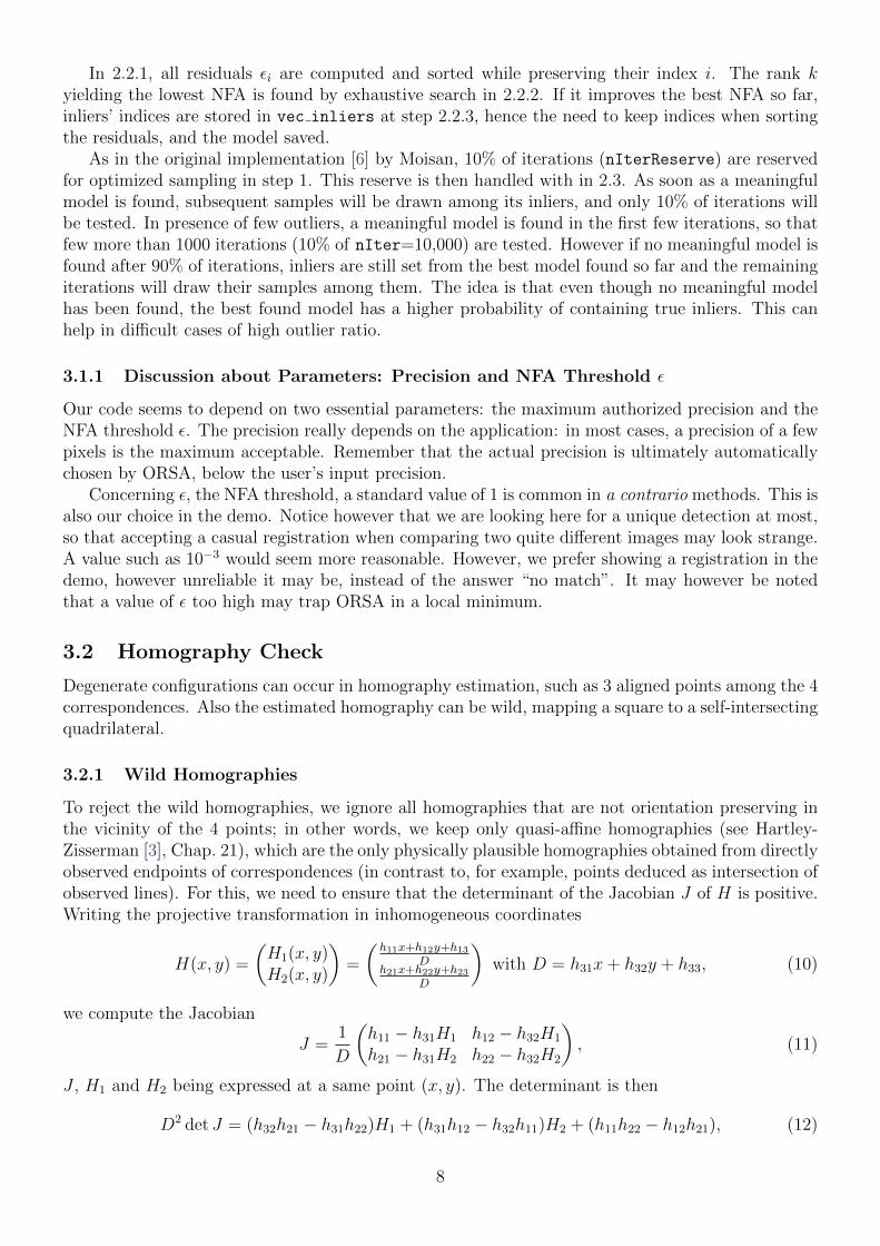
To reject the wild homographies, we ignore all homographies that are not orientation preserving inthe vicinity of the 4 points; in other words, we keep only quasi-affine homographies (see Hartley-Zisserman [3], Chap. 21), which are the only physically plausible homographies obtained from directlyobserved endpoints of correspondences (in contrast to, for example, points deduced as intersection ofobserved lines). For this, we need to ensure that the determinant of the Jacobian J of H is positive.Writing the projective transformation in inhomogeneous coordinates

H(x, y) =

(H1(x, y)H2(x, y)

)=

(h11x+h12y+h13

Dh21x+h22y+h23

D

)with D = h31x+ h32y + h33, (10)

we compute the Jacobian

J =1

D

(h11 − h31H1 h12 − h32H1

h21 − h31H2 h22 − h32H2

), (11)

J , H1 and H2 being expressed at a same point (x, y). The determinant is then

D2 det J = (h32h21 − h31h22)H1 + (h31h12 − h32h11)H2 + (h11h22 − h12h21), (12)

8

and we are interested in the positivity of the right hand side. It is interesting to note that theequation

(h32h21 − h31h22)x′ + (h31h12 − h32h11)y′ + (h11h22 − h12h21) = 0 (13)

represents the image of the line at infinity z = 0 in the right image (the image of a line l is H−T l

and the line at infinity is l∞ =(0 0 1

)T). More generally, the coefficients involved in the left hand

side are those of the last column of the comatrix of H, which, divided by det(H), is the last row ofH−1. Notice that if the 4 image points are on the positive side of this oriented line, so are points intheir convex hull.

Applying this constraint to H−1, we get

(h31x+ h32y + h33)/ det(h) > 0, (14)

for points (x, y) in the left image. It can be easily checked that if the latter constraint is satisfied, sois the former at corresponding point (x′, y′). Therefore, we check the positivity on the 4 left pointsbefore accepting the homography as physically plausible.

During computation of the error of the model, each correspondence not satisfying the aboveconstraint gets infinite error, so it cannot be counted as inlier.

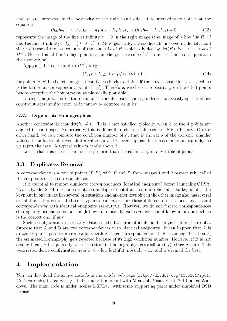
3.2.2 Degenerate Homographies

Another constraint is that det(h) 6= 0. This is not satisfied typically when 3 of the 4 points arealigned in one image. Numerically, this is difficult to check as the scale of h is arbitrary. On theother hand, we can compute the condition number of h, that is the ratio of the extreme singularvalues. In tests, we observed that a value above 10 never happens for a reasonable homography, sowe reject the case. A typical value is rarely above 3.

Notice that this check is simpler to perform than the collinearity of any triple of points.

3.3 Duplicates Removal

A correspondence is a pair of points (P, P ′) with P and P ′ from images 1 and 2 respectively, calledthe endpoints of the correspondence.

It is essential to remove duplicate correspondences (identical endpoints) before launching ORSA.Typically, the SIFT method can attach multiple orientations, so multiple codes, to keypoints. If akeypoint in one image has several orientations and another keypoint in the other image also has severalorientations, the codes of these keypoints can match for these different orientations, and severalcorrespondences with identical endpoints are output. However, we do not discard correspondencessharing only one endpoint: although they are mutually exclusive, we cannot know in advance whichis the correct one, if any.

Such a configuration is a clear violation of the background model and can yield dramatic results.Suppose that A and B are two correspondences with identical endpoints. It can happen that A isdrawn to participate to a trial sample with 3 other correspondences. If B is among the other 3,the estimated homography gets rejected because of its high condition number. However, if B is notamong them, B fits perfectly with the estimated homography (error=0 or tiny), since A does. This5-correspondence configuration gets a very low log(nfa), possibly −∞, and is deemed the best.

4 Implementation

You can download the source code from the article web page (http://dx.doi.org/10.5201/ipol.2012.mmm-oh), tested with g++ 4.6 under Linux and with Microsoft Visual C++ 2010 under Win-dows. The main code is under license LGPLv3, with some supporting parts under simplified BSDlicense.

9

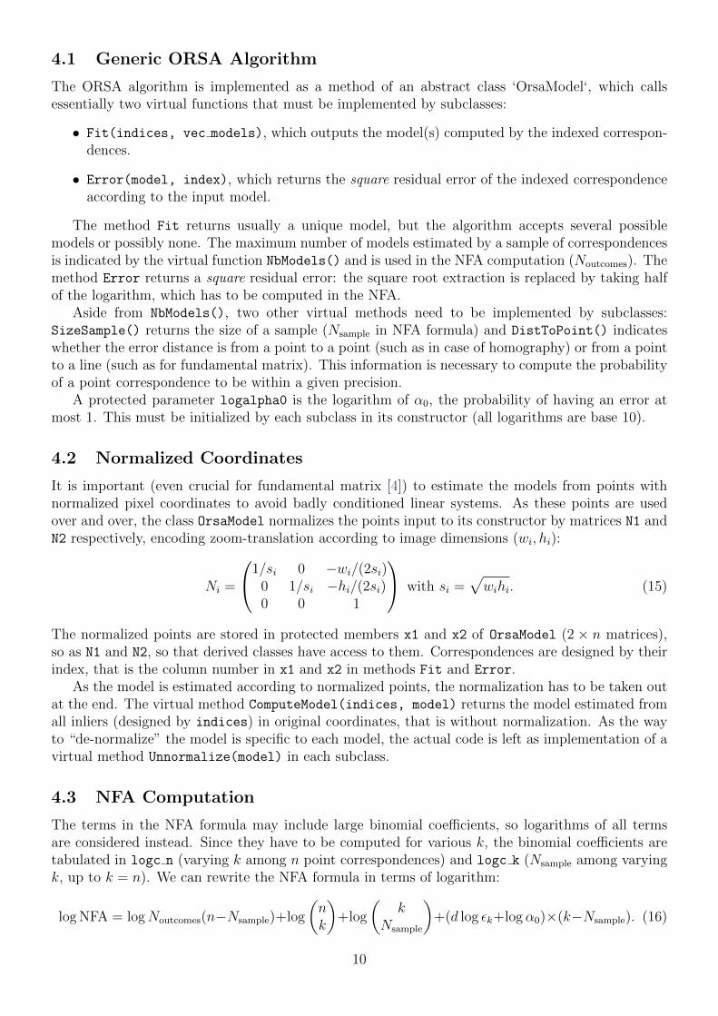
4.1 Generic ORSA Algorithm

The ORSA algorithm is implemented as a method of an abstract class ‘OrsaModel‘, which callsessentially two virtual functions that must be implemented by subclasses:

• Fit(indices, vec models), which outputs the model(s) computed by the indexed correspon-dences.

• Error(model, index), which returns the square residual error of the indexed correspondenceaccording to the input model.

The method Fit returns usually a unique model, but the algorithm accepts several possiblemodels or possibly none. The maximum number of models estimated by a sample of correspondencesis indicated by the virtual function NbModels() and is used in the NFA computation (Noutcomes). Themethod Error returns a square residual error: the square root extraction is replaced by taking halfof the logarithm, which has to be computed in the NFA.

Aside from NbModels(), two other virtual methods need to be implemented by subclasses:SizeSample() returns the size of a sample (Nsample in NFA formula) and DistToPoint() indicateswhether the error distance is from a point to a point (such as in case of homography) or from a pointto a line (such as for fundamental matrix). This information is necessary to compute the probabilityof a point correspondence to be within a given precision.

A protected parameter logalpha0 is the logarithm of α0, the probability of having an error atmost 1. This must be initialized by each subclass in its constructor (all logarithms are base 10).

4.2 Normalized Coordinates

It is important (even crucial for fundamental matrix [4]) to estimate the models from points withnormalized pixel coordinates to avoid badly conditioned linear systems. As these points are usedover and over, the class OrsaModel normalizes the points input to its constructor by matrices N1 andN2 respectively, encoding zoom-translation according to image dimensions (wi, hi):

Ni =

1/si 0 −wi/(2si)0 1/si −hi/(2si)0 0 1

with si =√wihi. (15)

The normalized points are stored in protected members x1 and x2 of OrsaModel (2 × n matrices),so as N1 and N2, so that derived classes have access to them. Correspondences are designed by theirindex, that is the column number in x1 and x2 in methods Fit and Error.

As the model is estimated according to normalized points, the normalization has to be taken outat the end. The virtual method ComputeModel(indices, model) returns the model estimated fromall inliers (designed by indices) in original coordinates, that is without normalization. As the wayto “de-normalize” the model is specific to each model, the actual code is left as implementation of avirtual method Unnormalize(model) in each subclass.

4.3 NFA Computation

The terms in the NFA formula may include large binomial coefficients, so logarithms of all termsare considered instead. Since they have to be computed for various k, the binomial coefficients aretabulated in logc n (varying k among n point correspondences) and logc k (Nsample among varyingk, up to k = n). We can rewrite the NFA formula in terms of logarithm:

log NFA = logNoutcomes(n−Nsample)+log

(nk

)+log

(k

Nsample

)+(d log εk+logα0)×(k−Nsample). (16)

10

The fixed term Noutcomes × (n−Nsample) involved in NFA has its log computed once as ‘loge0‘. Theactual NFA computation takes place in private method OrsaModel::bestNFA:

logalpha = logalpha0_ + multError *log10(e[k-1].first);

[...] loge0 + logalpha * (double)(k-startIndex) + logc_n[k] + logc_k[k] [...]

This is inside a loop with varying k (number of inliers), as in NFA formula. The term logalpha

is the log of the probability of having an error sqrt(e[k-1].first): remember that e[k-1].firstis the square error (k − 1 is the last among k inliers as numeration starts at 0). Its log is multipliedby multError (d = 2×multError), which is 1 or 0.5 depending on whether the error is distanceto a point (homography) or to a line (fundamental matrix), indicated by method DistToPoint().Indeed, in the first case the probability varies as the square of the error (area of a disk), while in thesecond case it varies linearly as the error, so we have to take square root of error, thus multiplyingthe log by 0.5.

The probability logalpha is multiplied by k-startIndex, which is k − Nsample. The binomialterms are added, so as the constant term loge0.

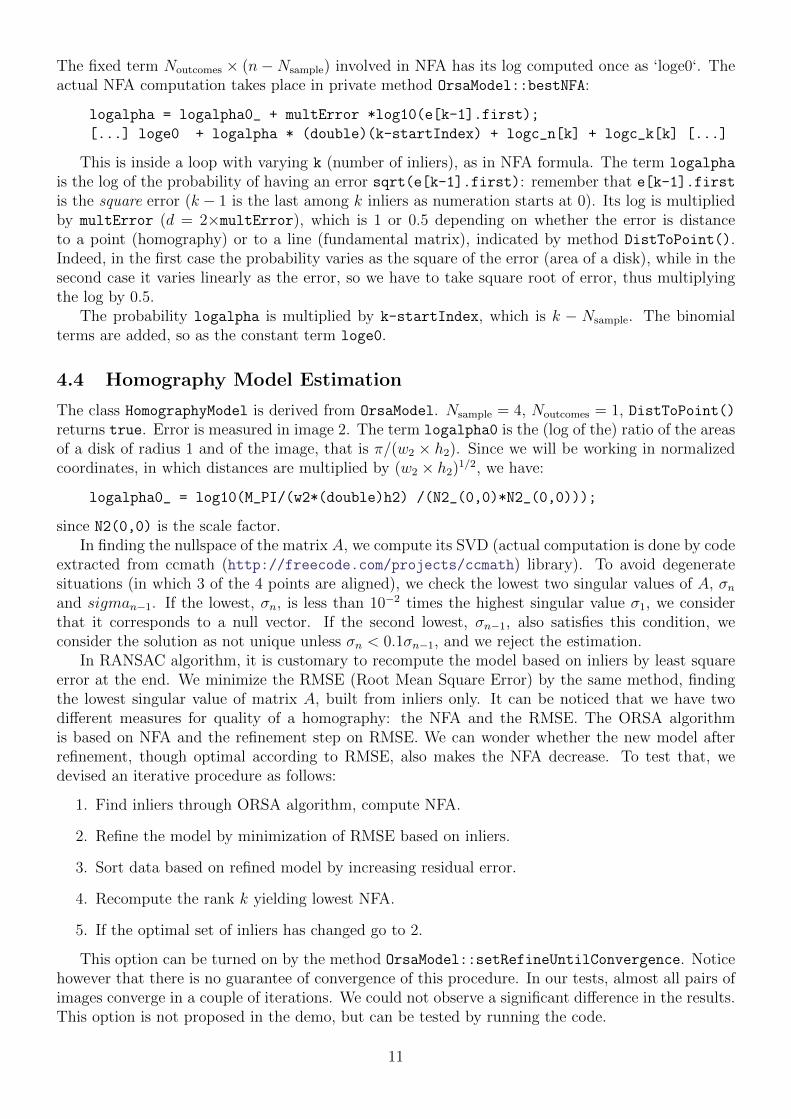
4.4 Homography Model Estimation

The class HomographyModel is derived from OrsaModel. Nsample = 4, Noutcomes = 1, DistToPoint()returns true. Error is measured in image 2. The term logalpha0 is the (log of the) ratio of the areasof a disk of radius 1 and of the image, that is π/(w2 × h2). Since we will be working in normalizedcoordinates, in which distances are multiplied by (w2 × h2)1/2, we have:

logalpha0_ = log10(M_PI/(w2*(double)h2) /(N2_(0,0)*N2_(0,0)));

since N2(0,0) is the scale factor.In finding the nullspace of the matrix A, we compute its SVD (actual computation is done by code

extracted from ccmath (http://freecode.com/projects/ccmath) library). To avoid degeneratesituations (in which 3 of the 4 points are aligned), we check the lowest two singular values of A, σnand sigman−1. If the lowest, σn, is less than 10−2 times the highest singular value σ1, we considerthat it corresponds to a null vector. If the second lowest, σn−1, also satisfies this condition, weconsider the solution as not unique unless σn < 0.1σn−1, and we reject the estimation.

In RANSAC algorithm, it is customary to recompute the model based on inliers by least squareerror at the end. We minimize the RMSE (Root Mean Square Error) by the same method, findingthe lowest singular value of matrix A, built from inliers only. It can be noticed that we have twodifferent measures for quality of a homography: the NFA and the RMSE. The ORSA algorithmis based on NFA and the refinement step on RMSE. We can wonder whether the new model afterrefinement, though optimal according to RMSE, also makes the NFA decrease. To test that, wedevised an iterative procedure as follows:

1. Find inliers through ORSA algorithm, compute NFA.

2. Refine the model by minimization of RMSE based on inliers.

3. Sort data based on refined model by increasing residual error.

4. Recompute the rank k yielding lowest NFA.

5. If the optimal set of inliers has changed go to 2.

This option can be turned on by the method OrsaModel::setRefineUntilConvergence. Noticehowever that there is no guarantee of convergence of this procedure. In our tests, almost all pairs ofimages converge in a couple of iterations. We could not observe a significant difference in the results.This option is not proposed in the demo, but can be tested by running the code.

11

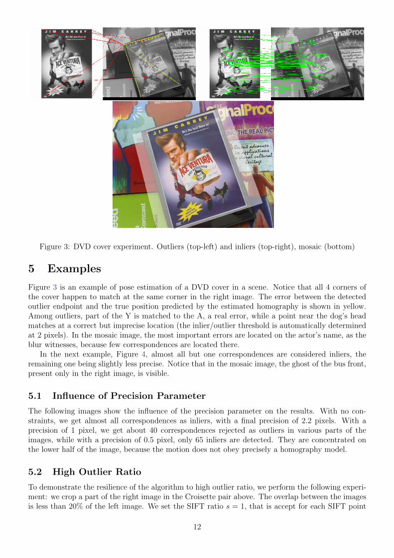
Figure 3: DVD cover experiment. Outliers (top-left) and inliers (top-right), mosaic (bottom)

5 Examples

Figure 3 is an example of pose estimation of a DVD cover in a scene. Notice that all 4 corners ofthe cover happen to match at the same corner in the right image. The error between the detectedoutlier endpoint and the true position predicted by the estimated homography is shown in yellow.Among outliers, part of the Y is matched to the A, a real error, while a point near the dog’s headmatches at a correct but imprecise location (the inlier/outlier threshold is automatically determinedat 2 pixels). In the mosaic image, the most important errors are located on the actor’s name, as theblur witnesses, because few correspondences are located there.

In the next example, Figure 4, almost all but one correspondences are considered inliers, theremaining one being slightly less precise. Notice that in the mosaic image, the ghost of the bus front,present only in the right image, is visible.

5.1 Influence of Precision Parameter

The following images show the influence of the precision parameter on the results. With no con-straints, we get almost all correspondences as inliers, with a final precision of 2.2 pixels. With aprecision of 1 pixel, we get about 40 correspondences rejected as outliers in various parts of theimages, while with a precision of 0.5 pixel, only 65 inliers are detected. They are concentrated onthe lower half of the image, because the motion does not obey precisely a homography model.

5.2 High Outlier Ratio

To demonstrate the resilience of the algorithm to high outlier ratio, we perform the following experi-ment: we crop a part of the right image in the Croisette pair above. The overlap between the imagesis less than 20% of the left image. We set the SIFT ratio s = 1, that is accept for each SIFT point

12

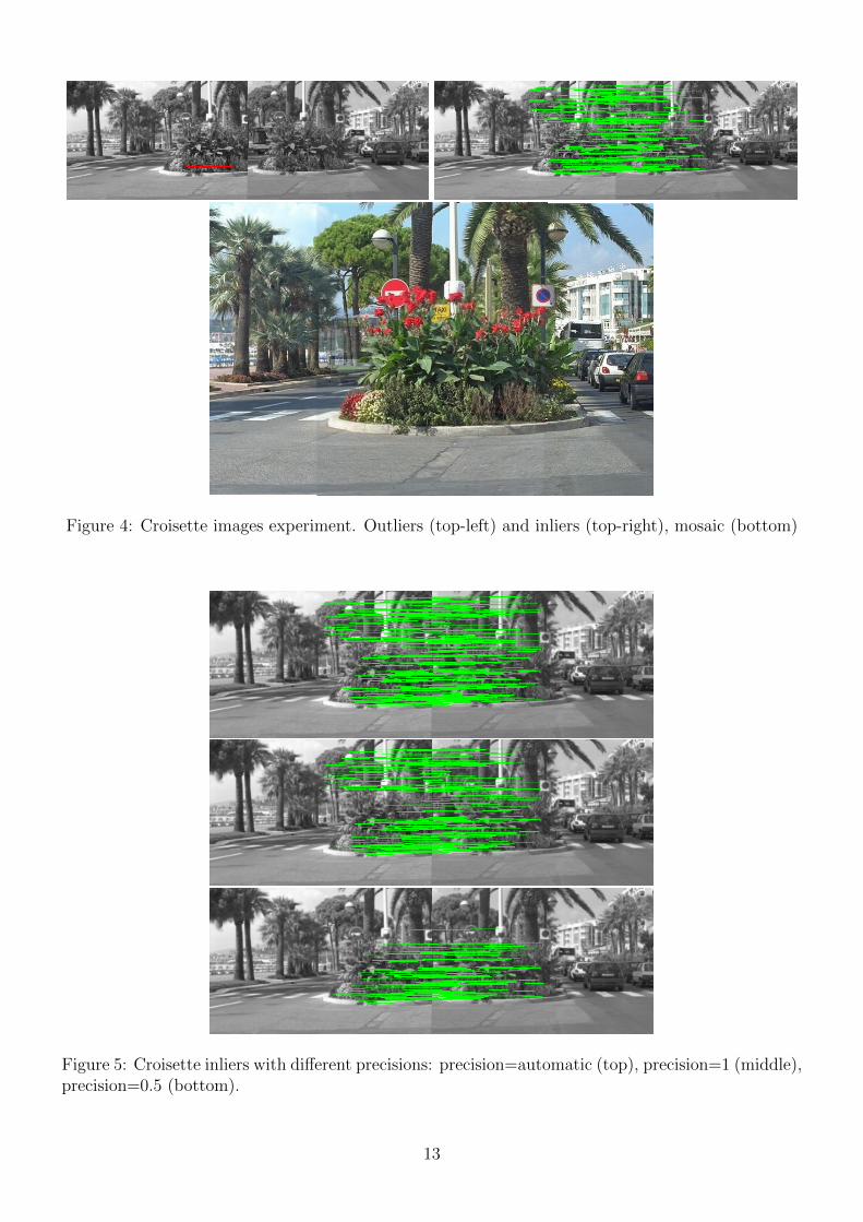
Figure 4: Croisette images experiment. Outliers (top-left) and inliers (top-right), mosaic (bottom)

Figure 5: Croisette inliers with different precisions: precision=automatic (top), precision=1 (middle),precision=0.5 (bottom).

13

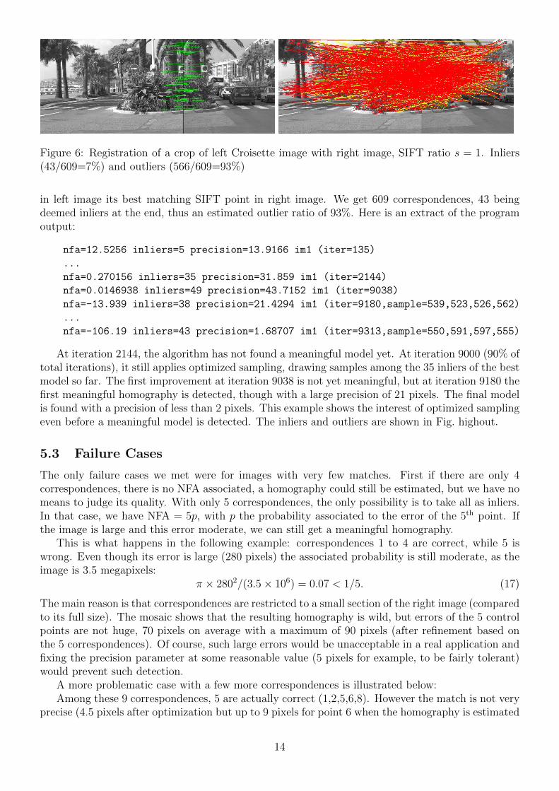
Figure 6: Registration of a crop of left Croisette image with right image, SIFT ratio s = 1. Inliers(43/609=7%) and outliers (566/609=93%)

in left image its best matching SIFT point in right image. We get 609 correspondences, 43 beingdeemed inliers at the end, thus an estimated outlier ratio of 93%. Here is an extract of the programoutput:

nfa=12.5256 inliers=5 precision=13.9166 im1 (iter=135)

...

nfa=0.270156 inliers=35 precision=31.859 im1 (iter=2144)

nfa=0.0146938 inliers=49 precision=43.7152 im1 (iter=9038)

nfa=-13.939 inliers=38 precision=21.4294 im1 (iter=9180,sample=539,523,526,562)

...

nfa=-106.19 inliers=43 precision=1.68707 im1 (iter=9313,sample=550,591,597,555)

At iteration 2144, the algorithm has not found a meaningful model yet. At iteration 9000 (90% oftotal iterations), it still applies optimized sampling, drawing samples among the 35 inliers of the bestmodel so far. The first improvement at iteration 9038 is not yet meaningful, but at iteration 9180 thefirst meaningful homography is detected, though with a large precision of 21 pixels. The final modelis found with a precision of less than 2 pixels. This example shows the interest of optimized samplingeven before a meaningful model is detected. The inliers and outliers are shown in Fig. highout.

5.3 Failure Cases

The only failure cases we met were for images with very few matches. First if there are only 4correspondences, there is no NFA associated, a homography could still be estimated, but we have nomeans to judge its quality. With only 5 correspondences, the only possibility is to take all as inliers.In that case, we have NFA = 5p, with p the probability associated to the error of the 5th point. Ifthe image is large and this error moderate, we can still get a meaningful homography.

This is what happens in the following example: correspondences 1 to 4 are correct, while 5 iswrong. Even though its error is large (280 pixels) the associated probability is still moderate, as theimage is 3.5 megapixels:

π × 2802/(3.5× 106) = 0.07 < 1/5. (17)

The main reason is that correspondences are restricted to a small section of the right image (comparedto its full size). The mosaic shows that the resulting homography is wild, but errors of the 5 controlpoints are not huge, 70 pixels on average with a maximum of 90 pixels (after refinement based onthe 5 correspondences). Of course, such large errors would be unacceptable in a real application andfixing the precision parameter at some reasonable value (5 pixels for example, to be fairly tolerant)would prevent such detection.

A more problematic case with a few more correspondences is illustrated below:Among these 9 correspondences, 5 are actually correct (1,2,5,6,8). However the match is not very

precise (4.5 pixels after optimization but up to 9 pixels for point 6 when the homography is estimated

14

Figure 7: Mosaic of Mogul images

15

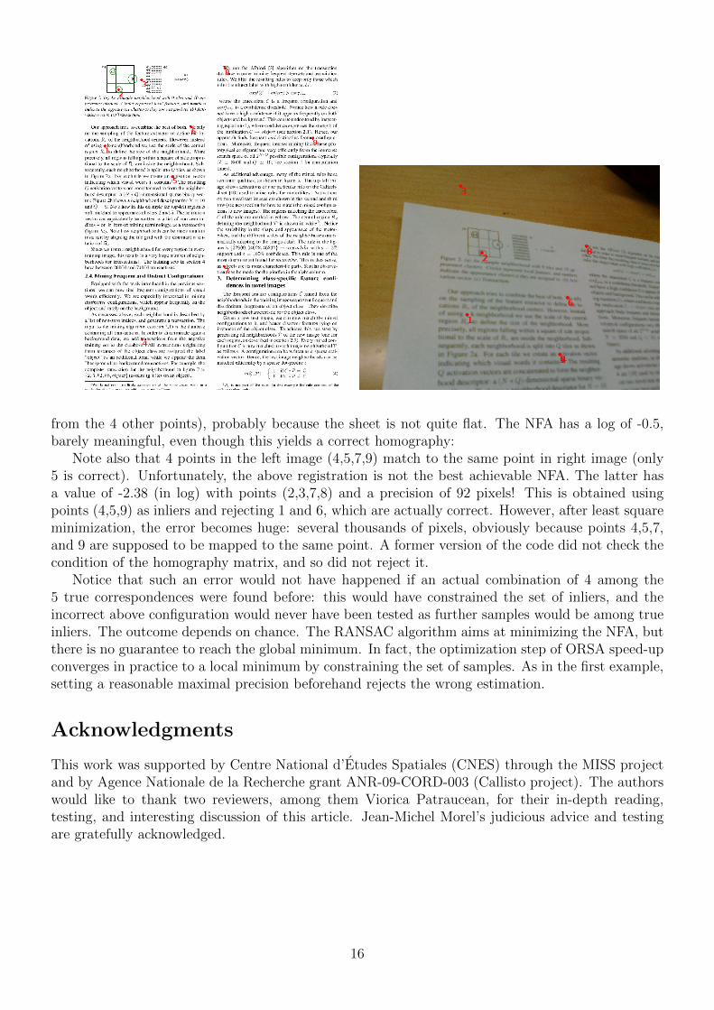
from the 4 other points), probably because the sheet is not quite flat. The NFA has a log of -0.5,barely meaningful, even though this yields a correct homography:

Note also that 4 points in the left image (4,5,7,9) match to the same point in right image (only5 is correct). Unfortunately, the above registration is not the best achievable NFA. The latter hasa value of -2.38 (in log) with points (2,3,7,8) and a precision of 92 pixels! This is obtained usingpoints (4,5,9) as inliers and rejecting 1 and 6, which are actually correct. However, after least squareminimization, the error becomes huge: several thousands of pixels, obviously because points 4,5,7,and 9 are supposed to be mapped to the same point. A former version of the code did not check thecondition of the homography matrix, and so did not reject it.

Notice that such an error would not have happened if an actual combination of 4 among the5 true correspondences were found before: this would have constrained the set of inliers, and theincorrect above configuration would never have been tested as further samples would be among trueinliers. The outcome depends on chance. The RANSAC algorithm aims at minimizing the NFA, butthere is no guarantee to reach the global minimum. In fact, the optimization step of ORSA speed-upconverges in practice to a local minimum by constraining the set of samples. As in the first example,setting a reasonable maximal precision beforehand rejects the wrong estimation.

Acknowledgments

This work was supported by Centre National d’Etudes Spatiales (CNES) through the MISS projectand by Agence Nationale de la Recherche grant ANR-09-CORD-003 (Callisto project). The authorswould like to thank two reviewers, among them Viorica Patraucean, for their in-depth reading,testing, and interesting discussion of this article. Jean-Michel Morel’s judicious advice and testingare gratefully acknowledged.

16

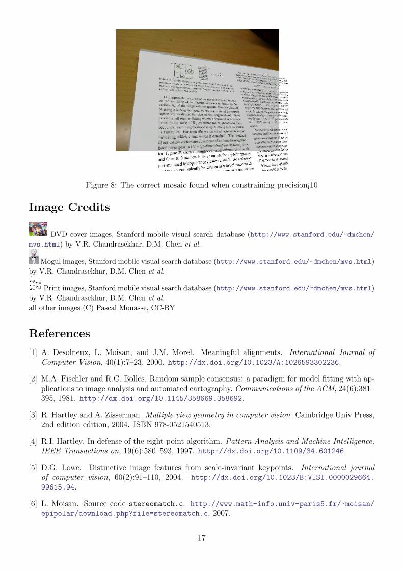
Figure 8: The correct mosaic found when constraining precision¡10

Image Credits

DVD cover images, Stanford mobile visual search database (http://www.stanford.edu/~dmchen/

mvs.html) by V.R. Chandrasekhar, D.M. Chen et al.

Mogul images, Stanford mobile visual search database (http://www.stanford.edu/~dmchen/mvs.html)

by V.R. Chandrasekhar, D.M. Chen et al.

Print images, Stanford mobile visual search database (http://www.stanford.edu/~dmchen/mvs.html)

by V.R. Chandrasekhar, D.M. Chen et al.

all other images (C) Pascal Monasse, CC-BY

References

[1] A. Desolneux, L. Moisan, and J.M. Morel. Meaningful alignments. International Journal ofComputer Vision, 40(1):7–23, 2000. http://dx.doi.org/10.1023/A:1026593302236.

[2] M.A. Fischler and R.C. Bolles. Random sample consensus: a paradigm for model fitting with ap-plications to image analysis and automated cartography. Communications of the ACM, 24(6):381–395, 1981. http://dx.doi.org/10.1145/358669.358692.

[3] R. Hartley and A. Zisserman. Multiple view geometry in computer vision. Cambridge Univ Press,2nd edition edition, 2004. ISBN 978-0521540513.

[4] R.I. Hartley. In defense of the eight-point algorithm. Pattern Analysis and Machine Intelligence,IEEE Transactions on, 19(6):580–593, 1997. http://dx.doi.org/10.1109/34.601246.

[5] D.G. Lowe. Distinctive image features from scale-invariant keypoints. International journalof computer vision, 60(2):91–110, 2004. http://dx.doi.org/10.1023/B:VISI.0000029664.

99615.94.

[6] L. Moisan. Source code stereomatch.c. http://www.math-info.univ-paris5.fr/~moisan/

epipolar/download.php?file=stereomatch.c, 2007.

17

[7] L. Moisan and B. Stival. A probabilistic criterion to detect rigid point matches between two imagesand estimate the fundamental matrix. International Journal of Computer Vision, 57(3):201–218,2004. http://dx.doi.org/10.1023/B:VISI.0000013094.38752.54.

[8] J. Rabin, J. Delon, Y. Gousseau, and L. Moisan. Mac-ransac: a robust algorithm for the recogni-tion of multiple objects. In Fifth International Symposium on 3D Data Processing, Visualizationand Transmission (3DPVT 2010), Paris: France, 2010.

18