Vertex Deletion Parameterized by Elimination Distance

and Even Less∗

Bart M. P. Jansen†

Eindhoven University of TechnologyJari J. H. de Kroon‡

Eindhoven University of Technology

Micha l W lodarczyk§

Eindhoven University of Technology

Abstract

We study the parameterized complexity of various classic vertex-deletion problems suchas Odd cycle transversal, Vertex planarization, and Chordal vertex deletionunder hybrid parameterizations. Existing FPT algorithms for these problems either focus onthe parameterization by solution size, detecting solutions of size k in time f(k) · nO(1), or widthparameterizations, finding arbitrarily large optimal solutions in time f(w) · nO(1) for some widthmeasure w like treewidth. We unify these lines of research by presenting FPT algorithms forparameterizations that can simultaneously be arbitrarily much smaller than the solution sizeand the treewidth.

The first class of parameterizations is based on the notion of elimination distance of the inputgraph to the target graph class H, which intuitively measures the number of rounds needed toobtain a graph in H by removing one vertex from each connected component in each round.The second class of parameterizations consists of a relaxation of the notion of treewidth, allowingarbitrarily large bags that induce subgraphs belonging to the target class of the deletion problemas long as these subgraphs have small neighborhoods. Both kinds of parameterizations havebeen introduced recently and have already spawned several independent results.

Our contribution is twofold. First, we present a framework for computing approximatelyoptimal decompositions related to these graph measures. Namely, if the cost of an optimaldecomposition is k, we show how to find a decomposition of cost kO(1) in time f(k) · nO(1).This is applicable to any class H for which the corresponding vertex-deletion problem admits aconstant-factor approximation algorithm or an FPT algorithm paramaterized by the solutionsize. Secondly, we exploit the constructed decompositions for solving vertex-deletion problemsby extending ideas from algorithms using iterative compression and the finite state property.For the three mentioned vertex-deletion problems, and all problems which can be formulated ashitting a finite set of connected forbidden (a) minors or (b) (induced) subgraphs, we obtain FPTalgorithms with respect to both studied parameterizations. For example, we present an algorithm

running in time nO(1) + 2kO(1) · (n+m) and polynomial space for Odd cycle transversalparameterized by the elimination distance k to the class of bipartite graphs.

∗This project has received funding from the European Research Council (ERC) under the European Union’s Horizon2020 research and innovation programme (grant agreement No 803421, ReduceSearch). An extended abstract [67] ofthis work appeared in the proceedings of the 53rd Symposium on Theory of Computing, STOC 2021.

†Address: b.m.p.jansen@tue.nl‡Address: j.j.h.d.kroon@tue.nl§Address: m.wlodarczyk@tue.nl

1

arX

iv:2

103.

0971

5v3

[cs

.DS]

10

Jan

2022

Contents

1 Introduction 3

2 Outline 82.1 Constructing decompositions . . . . . . . . . . . . . . . . . . . . . . . . . . . . . . . 82.2 Solving vertex-deletion problems . . . . . . . . . . . . . . . . . . . . . . . . . . . . . 10

3 Preliminaries 14

4 Constructing decompositions 174.1 From separation to decomposition . . . . . . . . . . . . . . . . . . . . . . . . . . . . 17

4.1.1 Constructing an H-elimination forest . . . . . . . . . . . . . . . . . . . . . . . 194.1.2 Restricted separation . . . . . . . . . . . . . . . . . . . . . . . . . . . . . . . . 214.1.3 Constructing a tree H-decomposition . . . . . . . . . . . . . . . . . . . . . . . 24

4.2 Finding separations . . . . . . . . . . . . . . . . . . . . . . . . . . . . . . . . . . . . . 264.2.1 Classes excluding induced subgraphs . . . . . . . . . . . . . . . . . . . . . . . 284.2.2 Bipartite graphs . . . . . . . . . . . . . . . . . . . . . . . . . . . . . . . . . . 294.2.3 Separation via packing-covering duality . . . . . . . . . . . . . . . . . . . . . 314.2.4 Finding restricted separations . . . . . . . . . . . . . . . . . . . . . . . . . . . 344.2.5 Disconnected obstructions . . . . . . . . . . . . . . . . . . . . . . . . . . . . . 35

4.3 Summary of the decomposition results . . . . . . . . . . . . . . . . . . . . . . . . . . 36

5 Solving vertex-deletion problems 395.1 Preliminaries for solving vertex-deletion problems . . . . . . . . . . . . . . . . . . . . 395.2 Incorporating hybrid parameterizations into existing algorithms . . . . . . . . . . . . 41

5.2.1 Odd cycle transversal . . . . . . . . . . . . . . . . . . . . . . . . . . . . . . . 415.2.2 Vertex cover . . . . . . . . . . . . . . . . . . . . . . . . . . . . . . . . . . . . 475.2.3 Hitting forbidden cliques . . . . . . . . . . . . . . . . . . . . . . . . . . . . . . 50

5.3 Generic algorithms via A-exhaustive families . . . . . . . . . . . . . . . . . . . . . . 515.3.1 A-exhaustive families and boundaried graphs . . . . . . . . . . . . . . . . . . 515.3.2 Dynamic programming with A-exhaustive families . . . . . . . . . . . . . . . 545.3.3 Hitting forbidden connected minors . . . . . . . . . . . . . . . . . . . . . . . 575.3.4 Hitting forbidden connected induced subgraphs . . . . . . . . . . . . . . . . . 595.3.5 Chordal deletion . . . . . . . . . . . . . . . . . . . . . . . . . . . . . . . . . . 615.3.6 Interval deletion . . . . . . . . . . . . . . . . . . . . . . . . . . . . . . . . . . 65

6 Hardness proofs 736.1 No FPT-approximation for perfect depth and width . . . . . . . . . . . . . . . . . . 736.2 Classes which are not closed under disjoint union . . . . . . . . . . . . . . . . . . . . 75

7 Conclusion 76

2

1 Introduction

The field of parameterized algorithmics [32, 35] develops fixed-parameter tractable (FPT) algorithmsto solve NP-hard problems exactly, which are provably efficient on inputs whose parameter value issmall. The purpose of this work is to unify two lines of research in parameterized algorithms forvertex-deletion problems that were previously mostly disjoint. On the one hand, there are algorithmsthat work on a structural decomposition of the graph, whose running time scales exponentiallywith a graph-complexity measure but polynomially with the size of the graph. Examples of suchalgorithms include dynamic programming over a tree decomposition [12, 15] (which forms a recursivedecomposition by small separators), dynamic-programming algorithms based on cliquewidth [31],rankwidth [63, 92, 93], and Booleanwidth [18] (which are recursive decompositions of a graph bysimply structured although not necessarily small separations). The second line of algorithms arethose that work with the “solution size” as the parameter, whose running time scales exponentiallywith the solution size. Such algorithms take advantage of the properties of inputs that admit smallsolutions. Examples of the latter include the celebrated iterative compression algorithm to finda minimum odd cycle transversal [97] and algorithms to compute a minimum vertex-deletion setwhose removal makes the graph chordal [26, 86], interval [24], or planar [68, 73, 87].

In this work we combine the best of both these lines of research, culminating in fixed-parametertractable algorithms for parameterizations which can be simultaneously smaller than naturalparameterizations by solution size and width measures like treewidth. To achieve this, we (1)employ recently introduced graph decompositions tailored to the optimization problem which willbe solved using the decomposition, (2) develop fixed-parameter tractable algorithms to computeapproximately optimal decompositions, and (3) show how to exploit the decompositions to obtainthe desired hybrid FPT algorithms. We apply these ideas to well-studied graph problems which canbe formulated in terms of vertex deletion: find a smallest vertex set whose removal ensures thatthe resulting graph belongs to a certain graph class. Vertex-deletion problems are among the mostprominent problems studied in parameterized algorithmics [27, 47, 60, 80, 83]. We develop newalgorithms for Odd cycle transversal, Vertex planarization, Chordal vertex deletion,and (induced) H-free deletion for fixed connected H, among others.

To be able to state our results, we give a high-level description of the graph decompositionswe employ; formal definitions are postponed to Section 3. Each decomposition is targeted ata specific graph class H. We use two types of decompositions, corresponding to relaxed versions oftreedepth [89] and treewidth [10, 99], respectively.

The first type of graph decompositions we employ are H-elimination forests, which decomposegraphs of bounded H-elimination distance. The H-elimination distance edH(G) of an undirectedgraph G is a graph parameter that was recently introduced [19, 20, 64], which admits a recursivedefinition similar to treedepth. If G is connected and belongs to H, then edH(G) = 0. If Gis connected but does not belong to H, then edH(G) = 1 + minv∈V (G) edH(G − v). If G hasmultiple connected components G1, . . . , Gp, then edH(G) = maxpi=1 edH(Gi). The process ofeliminating vertices in the second case of the definition explains the name elimination distance.The elimination process can be represented by a tree structure called an H-elimination forest,whose depth corresponds to edH(G). These decompositions can be used to obtain polynomial-spacealgorithms, similarly as for treedepth [8, 48, 95].

The second type of decompositions we employ are called tree H-decompositions, which decomposegraphs of bounded H-treewidth. These decompositions are obtained by relaxing the definition oftreewidth and were recently introduced by Eiben et al. [36], building on similar hybrid parameteriza-tions used in the context of solving SAT [53] and CSPs [54]. A tree H-decomposition of a graph Gis a tree decomposition of G, together with a set L ⊆ V (G) of base vertices. Base vertices are not

3

Figure 1: The vertex labels correspond to depth values in a bip-elimination forest of depth 5. Byattaching triangles to vertices of depth at most three, the minimum size of an odd cycle transversalcan increase boundlessly without increasing edbip. The vertices in yellow are the base vertices ofthe decomposition and induce a bipartite graph.

allowed to occur in more than one bag, and the base vertices in a bag must induce a subgraphbelonging to H. The connected components of G[L] are called the base components of the decompo-sition. The width of such a decomposition is defined as the maximum number of non-base verticesin any bag, minus one. A tree H-decomposition therefore represents a decomposition of a graph bysmall separators, into subgraphs which are either small or belong to H. The minimum width ofsuch a decomposition for G is the H-treewidth of G, denoted twH(G). We have twH(G) ≤ edH(G)for all graphs G, hence the former is a potentially smaller parameter. However, working with thisparameter will require exponential-space algorithms. We remark that both considered parame-terizations are interesting mainly for the case where the class H has unbounded treewidth, e.g.,H ∈ bipartite, chordal, planar, as otherwise twH(G) is comparable with tw(G) (see Lemma 3.6).Therefore we do not study classes such as trees or outerplanar graphs.

We illustrate the key ideas of the graph decomposition for the case of Odd cycle transversal(OCT), which is the vertex-deletion problem which aims to reach a bipartite graph. Hence OCTcorresponds to instantiations of the decompositions defined above for H being the class bip ofbipartite graphs. Observe that if G has an odd cycle transversal of k vertices, then edbip(G) ≤ k. Inthe other direction, the value edbip(G) may be arbitrarily much smaller than the size of a minimumOCT; see Figure 1. At the same time, the value of edbip(G) may be arbitrarily much smallerthan the rankwidth (and hence treewidth, cliquewidth, and treedepth) of G, since the n× n gridgraph is bipartite but has rankwidth n− 1 [70]. Hence a time bound of f(edbip(G)) · |G|O(1) canbe arbitrarily much better than bounds which are fixed-parameter tractable with respect to thesize of an optimal odd cycle transversal or with respect to pure width measures of G. Workingwith edbip as the parameter for Odd cycle transversal therefore facilitates algorithms whichsimultaneously improve on the solution-size [97] and width-based [82] algorithms for OCT. Asa sample of our results, we will prove that Odd cycle transversal can be solved in FPT-timeand polynomial space parameterized by edbip, and in FPT-time-and-space parameterized by twbip.Using this terminology, we now proceed to a detailed description of our contributions.

Results Our work advances the budding theory of hybrid parameterizations. The resultingframework generalizes and improves upon several isolated results in the literature. We presentthree types of theorems: FPT algorithms to compute approximate decompositions, FPT algorithms

4

employing these decompositions, and hardness results providing limits of tractability in this paradigm.While several results of the first and second kind have been known, we obtain the first frameworkwhich allows to handle miscellaneous graph classes with a unified set of techniques and to deliveralgorithms with a running time of the form 2k

O(1) ·nO(1), where k is either edH(G) or twH(G), evenif no decomposition is given in the input.

The following theorem1 gives a simple overview of our FPT-approximation algorithms for edHand twH. The more general version, as well as detailed results for concrete graph classes, can befound in Section 4.3.

Theorem 1.1. Let H be a hereditary union-closed class of graphs. Suppose that H-deletioneither admits a polynomial-time constant-factor approximation algorithm or an exact FPT algorithmparameterized by the solution size s, running in time 2s

O(1) · nO(1). There is an algorithm that,given an n-vertex graph G, computes in 2twH(G)O(1) · nO(1) time a tree H-decomposition of G ofwidth O(twH(G)5). Analogously, there is an algorithm that computes in 2edH(G)O(1) · nO(1) time anH-elimination forest of G of depth O(edH(G)3).

The prerequisites of the theorem are satisfied for classes of, e.g., bipartite graphs, chordal graphs,(proper) interval graphs, and graphs excluding a finite family of connected (a) minors or (b) inducedsubgraphs (see Table 2 in Section 4.3 for a longer list). In fact, the theorem is applicable also whenprovided with an FPT algorithm for H-deletion with an arbitrary dependency on the parameter.This is the case for classes of graphs excluding a finite family of connected topological minors,where we only know that the obtained dependency on twH(G) / edH(G) is a computable function.What is more, for some graph classes we are able to deliver algorithms with better approximationguarantees or running in polynomial time. Finally, we also show how to construct H-eliminationforests using only polynomial space at the expense of slightly worse approximation, which is laterleveraged in the applications.

While FPT algorithms to compute H-elimination distance for minor-closed graph classes H wereknown before [20] via an excluded-minor characterization (even to compute the exact distance), to thebest of our knowledge the general approach of Theorem 1.1 is the first to be able to (approximately)compute H-elimination distance for potentially dense target classes H such as chordal graphs.Concerning H-treewidth, we are only aware of a single prior result by Eiben et al. [36] which dealswith classes Hc consisting of the graphs of rankwidth at most c. To the best of our knowledge, ourresults for twH are the first to handle classes H of unbounded rankwidth2.

When considering graph classes defined by forbidden (topological) minors or induced subgraphs,Theorem 1.1 works only when all the obstructions are given by connected graphs due to therequirement that H must be union-closed. We show however that this connectivity assumptioncan be dropped and the same result holds for any graph class defined by a finite set of forbidden(topological) minors or induced subgraphs. In particular, we provide FPT-approximation algorithmsfor the class of split graphs (since they are characterized by a finite set of forbidden inducedsubgraphs) as well as for the class of interval graphs (since the corresponding vertex-deletionproblem admits a constant-factor approximation algorithm). This answers a challenge raised byEiben, Ganian, Hamm, and Kwon [36].

For the specific case of eliminating vertices to obtain a graph of maximum degree at most d ∈ O(1)(i.e., a graph which does not contain K1,d+1 or any of its spanning supergraphs as an inducedsubgraph), corresponding to the family H≤d of graphs of degree at most d, our algorithm runs

1This decomposition theorem strengthens the statements from the extended abstract [67], to be applicable whenevera suitable algorithm for the parameterization by solution size exists.

2Developments following the publication of the extended abstract of this article are given in “Related work”.

5

in time 2(edH≤d

(G))O(1)

· nO(1) and outputs a degree-d-elimination forest of depth O((edH≤d(G))2).

This improves on earlier work by Bulian and Dawar [19], who gave an FPT-algorithm with an

unspecified but computable parameter dependence to compute a decomposition of depth k2Ω(k)

for k = edH≤d(G).

We complement Theorem 1.1 by showing that, assuming FPT 6= W[1], no FPT-approximationalgorithms are possible for edperfect or twperfect, corresponding to perfect graphs.

By applying problem-specific insights to the problem-specific graph decompositions, we obtainFPT algorithms for vertex-deletion to H parameterized by edH and twH.

Theorem 1.2. Let H be a hereditary class of graphs that is defined by a finite number of forbiddenconnected (a) minors, or (b) induced subgraphs, or (c) H ∈ bipartite, chordal, interval. There is analgorithm that, given an n-vertex graph G, computes a minimum vertex set X such that G−X ∈ Hin time f(twH(G)) · nO(1).

As a consequence of case (a), for the class defined by the set of forbidden minors K5,K3,3 weobtain an algorithm for Vertex planarization parameterized by twplanar(G). In all cases the

running time is of the form 2kO(1) · nO(1), where k = twH(G). This is obtained by combining the

kO(1)-approximation from Theorem 1.1 with efficient algorithms working on given decompositions.For example, for H being the class of bipartite graphs, we present an algorithm for Odd cycle

transversal with running time 2O(k3) · nO(1) parameterized by k = twH(G). For H = chordal,the running time for Chordal deletion is 2O(k10) · nO(1). If H is defined by a family of connectedforbidden (induced) subgraphs on at most c vertices, we can solve H-deletion in time 2O(k6c) ·nO(1).Analogous statements with slightly better running times hold for parameterizations by edH(G),where in some cases we are additionally able to deliver polynomial-space algorithms.

All our algorithms are uniform: a single algorithm works for all values of the parameter. Usingan approach based on finite integer index introduced by Eiben et al. [36, Thm. 4], it is notdifficult to leverage the decompositions of Theorem 1.1 into non-uniform fixed-parameter tractablealgorithms for the corresponding vertex-deletion problems with an unknown parameter dependencein the running time. Our contribution in Theorem 1.2 therefore lies in the development of uniformalgorithms with concrete bounds on the running times.

For example, for the problem of deleting vertices to obtain a graph of maximum degree at most d

our running time is 2O(twH≤d

(G))6(d+1)

· nO(1). This improves upon a recent result by Ganian, Flute,and Ordyniak [49, Thm. 11], who gave an algorithm parameterized by the core fracture number k of

the graph whose parameter dependence is Ω(22(2k)k

). A graph with core fracture number k admitsan H≤d-elimination forest of depth at most 2k, so that the parameterizations by twH≤d

and edH≤d

can be arbitrarily much smaller and at most twice as large as the core fracture number.Intuitively, the use of decompositions in our algorithms is a strong generalization of the ubiqui-

tous idea of splitting a computation on a graph into independent computations on its connectedcomponents. Even if the components are not fully independent but admit limited interactionbetween them, via small vertex sets, Theorem 1.2 exploits this algorithmically. We consider thetheorem an important step in the quest to identify the smallest problem parameters that can explainthe tractability of inputs to NP-hard problems [43, 59, 91] (cf. [90, §6]). The theorem explains forthe first time how, for example, classes of inputs for Odd cycle transversal whose solution sizeand rankwidth are both large, can nevertheless be solved efficiently and exactly.

Not all classes H for which Theorem 1.1 yields decompositions, are covered by Theorem 1.2. Theproblem-specific adaptations needed to exploit the decompositions require significant technical work.In this article, we chose to focus on a number of key applications. We purposely restrict to the casewhere the forbidden induced subgraphs or minors are connected, as otherwise the problem does not

6

exhibit the behavior with “limited interaction between components” anymore. We formalize this inSection 6.2 with a proof that the respective H-deletion problem parameterized by either twH oredH is para-NP-hard. Regardless of that, we provide our decomposition theorems in full generality,as they may be of independent interest.

For some problems, we can leverage H-elimination forests to obtain polynomial-space analoguesof Theorem 1.2. For example, for the Odd cycle transversal problem we obtain an algorithmrunning in time nO(1) + 2edbip(G)O(1) · (n+m) and polynomial space. The additive behavior of therunning time comes from the fact that in this case, an approximate bip-elimination forest can becomputed in polynomial time, while the algorithm working on the decomposition is linear in n+m.

A result of a different kind is an FPT algorithm for Vertex cover parameterized by twH / edHfor H being any class for which Theorem 1.1 works and on which Vertex cover is solvable inpolynomial time. This means that Vertex cover is tractable on graphs with small H-treewidthfor H ∈ bipartite, chordal, claw-free. While this tractability was known when the input is givenalong with a decomposition [36], the fact that suitable decompositions can be computed efficientlyto establish tractability when given only a graph as input, is novel.

Related work Our results fall in a recent line of work of using hybrid parameterizations [19, 20,38, 39, 49, 50, 51, 53, 54, 55, 61] which simultaneously capture the connectivity structure of theinput instance and properties of its optimal solutions. Several of these works give decompositionalgorithms for parameterizations similar to ours; we discuss those which are most relevant.

Eiben, Ganian, Hamm, and Kwon [36] introduced the notion of H-treewidth and developedan algorithm to compute twrw≤c corresponding to H-treewidth where H is the class of graphs ofrankwidth at most c, for any fixed c. As the rankwidth rw(G) of any graph G satisfies rw(G) ≤c+ twrw≤c(G), their parameterization effectively bounds the rankwidth of the input graph, allowingthe use of model-checking theorems for Monadic Second Order Logic to compute a decomposition.In comparison, our Theorem 1.1 captures several classes of unbounded rankwidth such as bipartitegraphs and chordal graphs.

Eiben, Ganian, and Szeider [39] introduced the hybrid parameter H-well-structure number ofa graph G, which is a hybrid of the vertex-deletion distance to H and the rankwidth of a graph. Theygive FPT algorithms with unspecified parameter dependence f(k) to compute the correspondinggraph decomposition for classes H defined by a finite set of forbidden induced subgraphs, forests,and chordal graphs, and use this to solve Vertex cover parameterized by the H-well-structurenumber. Their parameterization is orthogonal to ours; for a class H of unbounded rankwidth,graphs of H-elimination distance 1 can have arbitrarily large H-well-structure number, as the lattermeasure is the sum rather than maximum over connected components that do not belong to H.

Ganian, Ramanujan, and Szeider [54] introduced a related hybrid parameterization in thecontext of constraint satisfaction problems, the backdoor treewidth. They show that if a certainset of variables X which allows a CSP to be decided quickly, called a strong backdoor, exists forwhich a suitable variant of treewidth is bounded for X, then such a set X can be computed in FPTtime. They use the technique of recursive understanding (cf. [29]) for this decomposition algorithm.This approach leads to a running time with a very quickly growing parameter dependence, at leastdoubly-exponential (cf. [52, Lemma 8]). After the conference version of this article was announced,several results employing recursive understanding to compute edH(G) for various classes H havebeen obtained [2, 3, 45, 66].

While the technique of recursive understanding and our decomposition framework both revolvearound repeatedly finding separations of a certain kind, the approaches are fundamentally different.The separations employed in recursive understanding are independent of the target class H and

7

always separate the graph into two large sides by a small separator. In comparison, the propertiesof the separations that our decomposition framework works with crucially vary with H. As a finalpoint of comparison, we note that our decomposition framework is sometimes able to deliver anapproximately optimal decomposition in polynomial time (for example, for the class H of bipartitegraphs), which is impossible using recursive understanding as merely finding a single reducibleseparation requires exponential time in the size of the separator.

Organization We start in Section 2 by providing an informal overview of our algorithmic contri-butions. In Section 3 we give formal preliminaries on graphs and complexity. There we also defineour graph decompositions. Section 4 shows how to compute approximate tree H-decompositionsand H-elimination forests for various graph classes H, building up to a proof of Theorem 1.1.The algorithms working on these decompositions are presented in Section 5, leading to a proof ofTheorem 1.2. In Section 6 we present two hardness results marking the boundaries of tractability.We conclude with a range of open problems in Section 7.

2 Outline

2.1 Constructing decompositions

We give a high-level overview of the techniques behind Theorem 1.1, which are generic and can beapplied in more settings than just those mentioned in the theorem. Theorem 1.2 requires solutionstailored for each distinct H, and will be discussed in Section 2.2.

The starting point for all algorithms to compute H-elimination forests or tree H-decompositions,is a subroutine to compute a novel kind of graph separation called (H, k)-separation, where k ∈ N.Such a separation in a graph G consists of a pair of disjoint vertex subsets (C, S) such that C inducesa subgraph belonging to H and consists of one or more connected components of G− S for someseparator S of size at most k. If there is an FPT-time (approximation) algorithm, parameterizedby k, for the problem of computing an (H, k)-separation (C, S) such that Z ⊆ C ∪ S for someinput set Z, then we show how to obtain algorithms for computing H-elimination forests and treeH-decompositions in a black-box manner. We use a four-step approach to approximate twH(G)and edH(G):

• Roughly speaking, given an initial vertex v chosen from the still-to-be decomposed part of thegraph, we iteratively apply the separation algorithm to find an (H, k)-separation (C 3 v, S)until reaching a separation whose set C cannot be extended anymore. We then compute apreliminary decomposition by repeatedly extracting such extremal (H, k)-separations (Ci, Si)from the graph.

• We use the extracted separations (Ci, Si) to define a partition of V (G) into connectedsets Vi ⊆ Ci ∪ Si. Then we define a contraction G′ of G, by contracting each connectedset Vi to a single vertex. The extremal property of the separations (Ci, Si) ensures that, apartfrom corner cases, the sets Vi cannot completely live in base components of an optimal treeH-decomposition or H-elimination forest. These properties of the preliminary decompositionwill enforce that the treewidth (respectively treedepth) of G′ is not much larger than twH(G)(respectively edH(G)).

• We invoke an exact [9, 98] or approximate [14, 34, 100] algorithm to compute the treewidth(respectively treedepth) of G′.

8

• Finally, we transform the tree decomposition (elimination forest) of G′ into a tree H-decomposition (H-elimination forest) of G without increasing the width (depth) too much.

The last step is more challenging for the case of constructing a tree H-decomposition. In orderto make it work, we need to additionally assume that the C-sides of the computed separationsdo not intersect too much. We introduce the notion of restricted separation that formalizes thisrequirement and work with a restricted version of the preliminary decomposition.

With the recipe above for turning (H, k)-separations into the desired graph decompositions, thechallenge remains to find such separations. We use several algorithmic approaches for various H.Table 2 on page 38 collects the results on obtaining H-elimination forests and tree H-decompositionsof moderate depth/width for various graph classes (formalized as theorems in Section 4.3).

For bipartite graphs, there is an elementary polynomial-time algorithm that given a graph Gand connected vertex set Z, computes a (H,≤ 2k)-separation (C ⊇ Z, S) if there exists a (H, k)-separation (C ′ ⊇ Z, S′). The algorithm is based on computing a minimum s− t vertex separator,using the fact that computing a vertex set S 63 v such that the component of G− S containing v isbipartite, can be phrased as separating an “even parity” copy of v from an “odd parity” copy of vin an auxiliary graph. Hence this variant of the (bip, k)-separation problem can be approximated inpolynomial time.

For other considered graph classes we present branching algorithms to compute approximateseparations in FPT time. For classes H defined by a finite set of forbidden induced subgraphs F ,we can find a vertex set F ⊆ V (G) such that G[F ] ∈ F in polynomial time, if one exists. If thereexists an (H, k)-separation (C, S) covering the given set Z, i.e., Z ⊆ C ∈ H and |S| ≤ k, then Fcannot be fully contained in C. To find a separation satisfying F ∩ S 6= ∅, we can guess a vertexin the intersection and recurse on a subproblem with k′ = k − 1. For separations with F ∩ S = ∅,some vertex v ∈ F lies in a different component of G− S than Z. We prove that in this case we canassume that S contains an important (v, Z)-separator of size ≤ k and we can branch on all suchimportant separators.

Our most general approach to finding (H, k)-separations relies on the packing-covering dualityof obstructions to H. It is known that graphs with bounded treewidth enjoy such a packing-coveringduality for connected obstructions for various graph classes [96]. We extend this observation tographs with bounded H-treewidth and obstructions to H. Namely, we show that when twH(G) ≤ kthen G contains either a vertex set X at most k(k+ 1) such that G−X ∈ H or k+ 1 vertex-disjointconnected subgraphs which do not belong to H.

In order to exploit this existential observation algorithmically, we again take advantage ofimportant separators. Suppose that there exists an (H, k)-separation (C, S) such that the givenvertex set Z is contained in C. In the first scenario, we rely on the existing algorithms for H-deletionto find an H-deletion set X. Even if the known algorithm is only a constant-factor approximation,it suffices to find X of size O(k2). Then the pair (V (G) \X,X) forms an (H,O(k2))-separation asdesired.

In the second scenario, by a counting argument there exists at least one obstruction to H whichis disjoint from S. This obstruction cannot be contained in C, so by connectivity it is disjoint fromC ∪ S. Then the set S forms a small separator between this obstruction and Z. By considering allvertices v ∈ V (G) \ Z and all important (v, Z)-separators of size at most k, we can detect such anobstruction – let us refer to it as F ⊆ V (G) – with a small boundary, i.e., |N(F )| ≤ k. There aretwo cases depending on whether F ∩ S = ∅. If so, we proceed similarly as for graph classes definedby forbidden induced subgraphs. Namely, we show that there exists an important (F,Z)-separatorof size ≤ k which is contained in S (for some feasible solution (C, S)) and we can perform branching.If F ∩S 6= ∅, then we take N(F ) into the solution and neglect F . Observe that in the remaining part

9

of the graph there exists an (H, k − 1)-separation (C∗, S∗) with Z ⊆ C∗. We have thus decreasedthe value of the parameter by one at the expense of paying the size of N(F ), which is at most k.This gives another branching rule. Combining these two rules yields a recursive algorithm whichoutputs an (H,O(k2))-separation.

2.2 Solving vertex-deletion problems

Here we provide an overview of the algorithms that work on the problem-specific decompositions.The results described above allow us to construct such decompositions of depth/width being apolynomial function of the optimal value, so in further arguments we can assume that a respectiveH-elimination forest or tree H-decomposition is given. For most applications of our framework, webuild atop existing algorithms that process (standard) elimination forests and tree decompositions.In order to make them work with the more general types of graph decomposition, we need tospecially handle the base components. To do this, we generalize arguments from the knownalgorithms parameterized by the solution size. An overview of the resulting running times for solvingH-deletion is given in Table 1.

We follow the ideas of gluing graphs and finite state property dating back to the results ofFellows and Langston [42] (cf. [5, 13]). We will present a meta-theorem which gives a recipe to solveH-deletion parameterized by H-treewidth or, as a corollary, by H-elimination distance. It worksfor any class which is hereditary, union-closed, and satisfies two technical conditions.

The first condition concerns the operation ⊕ of gluing graphs. Given two graphs with specifiedboundaries and an isomorphism between the boundaries, we can glue them along the boundariesby identifying the boundary vertices. Technical details aside, two boundaried graphs G1, G2

are equivalent with respect to H-membership if for any other boundaried graph H, we haveG1 ⊕H ∈ H ⇔ G2 ⊕H ∈ H. We say that the H-membership problem is finite state if the numberof such equivalence classes is finite for each boundary size k. We are interested in an upper boundrH(k), so that for every graph with boundary of size k one can find an equivalent graph on rH(k)vertices. In our applications, we are able to provide polynomial bounds on rH(k), which could besignificantly harder for the approach based on finite integer index [16, 36]. Before describing howto bound rH(k), we first explain how such a bound can lead to an algorithm parameterized bytreewidth.

Each bag of a tree decomposition forms a small separator. Consider a bag Xt ⊆ V (G) of size kand set At ⊆ V (G) of vertices introduced in the subtree of node t. Then the subgraph Gt inducedby vertices At ∪Xt has a natural small boundary Xt. Suppose that for two subsets S1, S2 ⊆ At ∪Xt,we have S1 ∩Xt = S2 ∩Xt and the boundaried graphs Gt − S1, Gt − S2 are equivalent with respectto H-membership. Then S1 are S2 are equally good for the further choices of the algorithm: ifsome set S′ ⊆ V (G) \ (At ∪Xt) extends S1 to a valid solution, the same holds for S2. If we canenumerate all equivalence classes for H-membership, we could store at each node t of the treedecomposition and each equivalence class C, the minimum size of a deletion set S within Gt sothat Gt − S ∈ C; this provides sufficient information for a dynamic-programming routine. Such anapproach has been employed to design optimal algorithms solving H-deletion parameterized bytreewidth for minor-closed classes [6].

We modify this idea to additionally handle the base components, which are arbitrarily largesubgraphs that belong to H stored in the leaves of a tree H-decomposition or H-elimination forest,and which are separated from the rest of the graph by a vertex set Xt whose size is bounded bythe cost k of the decomposition. This separation property ensures that any optimal solution Sto H-deletion contains at most k vertices from a base component At, as otherwise we could replaceAt ∩ S by Xt to obtain a smaller solution. This means that in principle, we can afford to use an

10

algorithm for the parameterization by the solution size and run it with the cost value k of thedecomposition. However, such an algorithm does not take into account the connections between thebase component and the rest of the graph. If we wanted to take this into account by computinga minimum-size deletion set St in a base component At for which G[At ∪ Xt] − St belongs to agiven equivalence class C, we would need a far-reaching generalization of the algorithm solvingH-deletion parameterized by the solution size. Working with a variant of the deletion problemthat supports undeletable vertices allows us to alleviate this issue. We enumerate the minimalrepresentatives of all the equivalence classes. Then, given a bag Xt and the base component At, weconsider all subsets Xs ⊆ Xt and perform gluing G′ = G[At ∪ (Xt \Xs)] with each representative Ralong Xt \Xs. One of the representatives R is equivalent to the graph G−At−S, with the boundaryXt \ S, where S is the optimal solution. Therefore, the set S ∩ At is a solution to H-deletionfor the graph G′ ⊕R and any subset SRt ⊆ At with this property can be extended to a solution inG using the vertices from S \ (At ∪Xt). Since we can assume that |S ∩ At| is at most the widthof the decomposition, we can find its replacement SRt ⊆ At of minimum size as long as we cansolve H-deletion with some vertices marked as undeletable, parameterized by the solution size.This constitutes the second condition for H. We check that for all studied problems, the knownalgorithms can be adapted to work in this setting.

The generic dynamic programming routine works as follows. First, we generate the minimalrepresentatives of the equivalence classes with respect to H-membership. The size of this familyis governed by the bound rH(k), which differs for various classes H. For each base component Atand for each representative R, we perform the gluing operation, compute a minimum-size subsetSRt ⊆ At that solves H-deletion on the obtained graph, and add it to a family St. Then for anyoptimal solution S, there exists St ∈ St such that (S \At) ∪ St is also an optimal solution. Such afamily of partial solutions for At ⊆ V (G) is called At-exhaustive. We proceed to compute exhaustivefamilies bottom-up in a decomposition tree, combining exhaustive families for children by bruteforce to get a new exhaustive family for their parent, and then trim the size of that family so itnever grows too large. The following theorem summarizes our meta-approach.

Theorem 2.1. Suppose that the class H is hereditary and union-closed. Furthermore, assume that H-deletion with undeletable vertices admits an algorithm with running time f(k)·nO(1), where k is thesolution size. Then H-deletion on an n-vertex graph G can be solved in time f(k)·2O(rH(k)2+k)·nO(1)

when given a tree H-decomposition of G of width k consisting of nO(1) nodes.

If the class H is defined by a finite set of forbidden connected minors, we can take advantage ofthe theorem by Baste, Sau, and Thilikos [6] which implies that rH(k) = OH(k), and a constructionby Sau, Stamoulis, and Thilikos [103] to solve H-deletion with undeletable vertices. Combining

these results with our framework gives an algorithm running in time 2kO(1) · nO(1) for parameter

k = twH(G). For other classes we first need to develop some theory to make them amenable to themeta-theorem.

Chordal deletion We explain briefly how the presented framework allows us to solve Chordaldeletion when given a tree chordal-decomposition. The upper bound rchordal(k) on the sizes ofrepresentatives comes from a new characterization of chordal graphs. Consider a boundaried chordalgraph G with a boundary X of size k. We define the condensing operation, which contracts edgeswith both endpoints in V (G) \X and removes vertices from V (G) \X which are simplicial (a vertexis simplicial if its neighborhood is a clique). Let G be obtained by condensing G. We prove that Gand G are equivalent with respect to chordal−membership, that is, for any other boundaried graphH, the result of gluing H ⊕G gives a chordal graph if and only H ⊕ G is chordal. Furthermore, we

11

show that after condensing there can be at most O(k) vertices in G, which implies rchordal(k) = O(k).As a result, there can be at most 2O(rchordal(k)2) = 2O(k2) equivalence classes of graphs with boundaryat most k.

The second required ingredient is an algorithm for Chordal deletion with undeletable ver-tices, parameterized by the solution size k. We provide a simple reduction to the standardChordal deletion problem, which admits an algorithm with running time 2O(k log k) · nO(1) [26].Our construction directly implies that Chordal deletion on graphs of (standard) treewidth k canbe solved in time 2O(k2) · nO(1). To the best of our knowledge, this is the first explicit treewidth-DPfor Chordal deletion; previous algorithms all relied on Courcelle’s theorem.

Together with the FPT-approximation algorithm for computing a tree chordal-decomposition,we obtain (Corollary 5.63) an algorithm solving Chordal deletion in time 2O(k10) · nO(1) whenparameterized by k = twchordal(G).

Interval deletion In order to solve Interval deletion with a given tree interval-decomposition,we need to bound the function rinterval(k). A graph G is interval if and only if G is chordal and Gdoes not contain an asteroidal triple (AT), that is, a triple of vertices so that for any two of themthere is a path between them avoiding the closed neighborhood of the third. As we have alreadydeveloped a theory to understand chordal−membership, the main task remains to identify graphmodifications which preserve the structure of asteroidal triples. We show that given a boundariedinterval graph G with boundary X of size k, we can mark a set Q ⊆ V (G) of size kO(1) so that forany result of gluing F = H ⊕G, if F contains some AT, then F contains an AT (w1, w2, w3) so thatw1, w2, w3 ∩ V (G) ⊆ X ∪Q. Afterwards, the vertices from V (G) \ (X ∪Q) can be either removedor contracted together, so that in the end we obtain a boundaried graph G′ of size kO(1) which isequivalent to G with respect to interval−membership.

As the most illustrative case of the marking scheme, consider vertices v1, v2, v3 ∈ V (G), suchthat there exists a (v1, v2)-path P in the graph F − NF [v3]. Recall that F = H ⊕ G, where His an unknown boundaried graph. Intuitively, the marking scheme tries to enumerate all ways inwhich P crosses the boundary X of G. The naive way would be to enumerate each ordered subsetof X and consider paths which visit these vertices of X in the given order. There are Ω(k!) suchcombinations though. Instead, we fix an interval model of G and show that only O(1) subpaths ofP on the G-side of X are relevant. These are the subpaths closest to the vertices v1, v2, v3 in theinterval model. This allows us to define a signature of path P with the following properties: (1)if there exists another triple w1, w2, w3 ∈ V (G) which matches the signature, then there exists a(w1, w2)-path P ′ in the graph F −NF [w3] and (2) there are only kO(1) different signatures. For anytriple of signatures, representing respectively (v1, v2)-path, (v2, v3)-path, and (v3, v1)-path, we checkif there exists a triple of vertices that matches all of them (modulo ordering). If yes, we mark thevertices in any such triple. This procedure marks a set Q ⊆ V (G) of kO(1) vertices, as intended.

Similarly as for Chordal deletion, we adapt the algorithm for Interval deletion parame-terized by the solution size [25] to work with undeletable vertices. Together, this makes Intervaldeletion amenable to our framework (Corollary 5.82).

Hitting connected forbidden induced subgraphs We use the same approach to solve H-deletion when H is defined by a finite set F of connected forbidden induced subgraphs on at most cvertices each. The standard technique of bounded-depth branching provides an FPT algorithm forthe parameterization by solution size in the presence of undeletable vertices. We prove an upperbound rH(k) = O(kc) and obtain running time 2O(k6c) · nO(1), where k = twH(G) (Corollary 5.49).

In the special case when H is defined by a single forbidden induced subgraph that is a clique Kt,

12

we can additionally obtain (Corollary 5.24) a polynomial-space algorithm for the parameterizationby k = edH, which runs in time 2O(k3 log k) · nO(1). Here the key insight is that a forbidden clique isrepresented on a single root-to-leaf path of an H-elimination forest, allowing for a polynomial-spacebranching step that avoids the memory-intensive dynamic-programming technique.

When the forbidden clique Kt has size two, then we obtain the Vertex cover problem. Thefamily H of K2-free graphs is simply the class of edge-less graphs, and the elimination distanceto an edge-less graph is not a smaller parameter than treedepth or treewidth. But for Vertexcover we can work with even more relaxed parameterizations. For H defined by a finite set offorbidden induced subgraphs such that Vertex cover is polynomial-time solvable on graphsfrom H (for example, claw-free graphs), or H ∈ chordal, bipartite (for which Vertex cover isalso polynomial-time solvable), we can find a minimum vertex cover in FPT time parameterizedby edH (Corollary 5.19) and twH (Corollary 5.21). In the former case, the algorithm even works inpolynomial space. More generally, Vertex cover is FPT parameterized by edH and twH for anyhereditary class H on which the problem is polynomial, when a decomposition is given in the input.

Odd cycle transversal While this problem can be shown to fit into the framework of Theorem 2.1,we provide specialized algorithms with improved guarantees. Given a tree bip-decomposition ofwidth k, we can solve the problem in time 2O(k) · nO(1) (Theorem 5.16) by utilizing a subroutinedeveloped for iterative compression [97]. What is more, we obtain the same time bound withinpolynomial space when given a bip-elimination forest of depth k. Below, we describe how theiterative-compression subroutine is used in the latter algorithm.

Suppose we are given a vertex set S ⊆ V (G) that separates G into connected componentsC1, . . . , Cp. The optimal solution may remove some subset SX ⊆ S and the vertices in S \ SX canthen be divided into 2 groups S1, S2 reflecting the 2-coloring of the resulting bipartite graph. If|S| ≤ d, then there are 3d choices to split S into (S1, S2, SX). We can consider all of them andsolve the problem recursively on C1 ∪ S, . . . , Cp ∪ S, restricting to the solutions coherent with thepartition of (S1, S2, SX). We call such a subproblem with restrictions an annotated problem.

A standard elimination forest provides us with a convenient mechanism of separators, given bythe node-to-root paths, to be used in the scheme above. The length of each such path is boundedby the depth d of the elimination forest, so we can solve the problem recursively, starting from theseparation given by the root node, in time O(3d · dO(1) · n) when given a depth-d elimination forest.Moreover, such a computation needs only to keep track of the annotated vertices in each recursivecall, so it can be implemented to run in polynomial space.

If we replace the standard elimination forest with a bip-elimination forest, the idea is analogousbut we need to additionally take care of the base components. In each such subproblem we are givena bipartite component C, a partition (S1, S2, SX) of N(C), and want to find a minimal set CX ⊆ Cso that C − CX is coherent with (S1, S2, SX): that is, there is no even path from u ∈ S1 to v ∈ S2

and no odd path between vertices from each Si. It turns out that the same subproblem occurs inthe algorithm for Odd cycle transversal parameterized by the solution size in a single step initerative compression. This problem, called Annotated bipartite coloring, can be reduced tofinding a minimum cut and is solvable in polynomial-time. Furthermore, we can assume that CX isat most as large as the depth of the given bip-elimination forest, because otherwise we could removethe set N(C) instead of CX and obtain a smaller solution. This observation allows us to improvethe running time to be linear in n+m (Corollary 5.15), so that given a graph G of bip-eliminationdistance k we can compute a minimum odd cycle transversal in nO(1) + 2O(k3 log k) · (n+m) timeand polynomial space by using a polynomial-space algorithm to construct a bip-elimination forest.

13

Table 1: Running times for solving H-Deletion parameterized by edH and twH. The algorithms only needthe graph G as input and construct a decomposition within the same time bounds.

class H k = twH k = edHbipartite 2O(k3) · nO(1) nO(1) + 2O(k3 log k) · (n+m)

chordal 2O(k10) · nO(1) 2O(k6) · nO(1)

interval 2kO(1) · nO(1) 2k

O(1) · nO(1)

planar 2O(k10 log k) · nO(1) 2O(k6 log k) · nO(1)

forbidden connected minors 2kO(1) · nO(1) 2k

O(1) · nO(1)

forbidden connected induced subgraphs

on ≤ c vertices 2O(k6c) · nO(1) 2O(k4c) · nO(1)

forbidden clique Kt 2O(k6t) · nO(1) 2O(k3 log k) · nO(1)

3 Preliminaries

The set 1, . . . , p is denoted by [p]. For a finite set S, we denote by 2S the powerset of Sconsisting of all its subsets. For n ∈ N we use Sn to denote the set of n-tuples over S. Weconsider simple undirected graphs without self-loops. A graph G has vertex set V (G) and edgeset E(G). We use shorthand n = |V (G)| and m = |E(G)|. For disjoint A,B ⊆ V (G), we defineEG(A,B) = uv | u ∈ A, v ∈ B, uv ∈ E(G), where we omit subscript G if it is clear from context.For A ⊆ V (G), the graph induced by A is denoted by G[A] and we say that the vertex set A isconnected if the graph G[A] is connected. We use shorthand G − A for the graph G[V (G) \ A].For v ∈ V (G), we write G − v instead of G − v. The open neighborhood of v ∈ V (G) isNG(v) := u | uv ∈ E(G), where we omit the subscript G if it is clear from context. For a vertexset S ⊆ V (G) the open neighborhood of S, denoted NG(S), is defined as

⋃v∈S NG(v)\S. The closed

neighborhood of a single vertex v is NG[v] := NG(v) ∪ v, and the closed neighborhood of a vertexset S is NG[S] := NG(S) ∪ S. For two disjoint sets X,Y ⊆ V (G), we say that S ⊆ V (G) \ (X ∪ Y )is an (X,Y )-separator if the graph G− S does not contain any path from any u ∈ X to any v ∈ Y .

For graphs G and H, we write G ⊆ H to denote that G is a subgraph of H. A tree is a connectedgraph that is acyclic. A forest is a disjoint union of trees. In tree T with root r, we say that t ∈ V (T )is an ancestor of t′ ∈ V (T ) (equivalently t′ is a descendant of t) if t lies on the (unique) path from rto t′. A graph G admits a proper q-coloring, if there exists a function c : V (G) → [q] such thatc(u) 6= c(v) for all uv ∈ E(G). A graph is bipartite if and only if it admits a proper 2-coloring.A graph is chordal if it does not contain any induced cycle of length at least four. A graph is aninterval graph if it is the intersection graph of a set of intervals on the real line. It is well-knownthat all interval graphs are chordal (cf. [17]).

Let RGS (X) be the set of vertices reachable from X \ S in G− S, where superscript G is omittedif it is clear from context.

Definition 3.1 ([32]). Let G be a graph and let X,Y ⊆ V (G) be two disjoint sets of vertices. LetS ⊆ V (G) \ (X ∪ Y ) be an (X,Y )-separator. We say that S is an important (X,Y )-separator if itis inclusion-wise minimal and there is no (X,Y )-separator S′ ⊆ V (G) \ (X ∪ Y ) such that |S′| ≤ |S|and RGS (X) ( RGS′(X).

Lemma 3.2 ([32, Proposition 8.50]). Let G be a graph and X,Y ⊆ V (G) be two disjoint sets ofvertices. Let S ⊆ V (G)\(X∪Y ) be an (X,Y )-separator. Then there is an important (X,Y )-separatorS′ = NG(RGS′(X)) such that |S′| ≤ |S| and RGS (X) ⊆ RGS′(X).

14

Contractions and minors A contraction of uv ∈ E(G) introduces a new vertex adjacent to allof N(u, v), after which u and v are deleted. The result of contracting uv ∈ E(G) is denoted G/uv.For A ⊆ V (G) such that G[A] is connected, we say we contract A if we simultaneously contract alledges in G[A] and introduce a single new vertex.

We say that H is a contraction of G, if we can turn G into H by a series of edge contractions.Furthermore, H is a minor of G, if we can turn G into H by a series of edge contractions, edgedeletions, and vertex deletions. We can represent the result of such a process with a mappingφ : V (H)→ 2V (G), such that subgraphs (G[φ(h)])h∈V (H) are connected and vertex-disjoint, with anedge of G between a vertex in φ(u) and a vertex in φ(v) for all uv ∈ E(H). The sets φ(h) are calledbranch sets and the family (φ(h))h∈V (H) is called a minor-model of H in G. A family (φ(h))h∈V (H)

of branch sets is called a contraction-model of H in G if the sets (φ(h))h∈V (H) partition V (G) andfor each pair of distinct vertices u, v ∈ V (H) we have uv ∈ E(H) if and only if there is an edge in Gbetween a vertex in φ(u) and a vertex in φ(v).

A subdivision of an edge uv is an operation that replaces the edge uv with a vertex w connectedto both u and v. We say that graph G is a subdivision of H if H can be transformed into G bya series of edge subdivisions. A graph H is called a topological minor of G if there is a subgraph ofG being a subdivision of H. Note that this implies that H is also a minor of G, but the implicationin the opposite direction does not hold.

Graph classes and decompositions We always assume that H is a hereditary class of graphs,that is, closed under taking induced subgraphs. A set X ⊆ V (G) is called an H-deletion set ifG−X ∈ H. The task of finding a smallest H-deletion set is called the H-deletion problem (alsoreferred to as H-vertex deletion, but we abbreviate it since we do not consider edge deletionproblems). When parameterized by the solution size k, the task for the H-deletion problem is toeither find a minimum-size H-deletion set or report that no such set of size at most k exists. Wesay that class H is union-closed if a disjoint union of two graphs from H also belongs to H.

Definition 3.3. For a graph class H, an H-elimination forest of graph G is pair (T, χ) where T isa rooted forest and χ : V (T )→ 2V (G), such that:

1. For each internal node t of T we have |χ(t)| = 1.

2. The sets (χ(t))t∈V (T ) form a partition of V (G).

3. For each edge uv ∈ E(G), if u ∈ χ(t1) and v ∈ χ(t2) then t1, t2 are in ancestor-descendantrelation in T .

4. For each leaf t of T , the graph G[χ(t)], called a base component, belongs to H.

The depth of T is the maximum number of edges on a root-to-leaf path. We refer to the union ofbase components as the set of base vertices. The H-elimination distance of G, denoted edH(G), isthe minimum depth of an H-elimination forest for G. A pair (T, χ) is a (standard) eliminationforest if H is the class of empty graphs, i.e., the base components are empty. The treedepth of G,denoted td(G), is the minimum depth of a standard elimination forest.

It is straight-forward to verify that for any G and H, the minimum depth of an H-eliminationforest of G is equal to the H-elimination distance as defined recursively in the introduction. (This isthe reason we have defined the depth of an H-elimination forest in terms of the number of edges,while the traditional definition of treedepth counts vertices on root-to-leaf paths.)

The following definition captures our relaxed notion of tree decomposition.

15

Definition 3.4. For a graph class H, a tree H-decomposition of graph G is a triple (T, χ, L)where L ⊆ V (G), T is a rooted tree, and χ : V (T )→ 2V (G), such that:

1. For each v ∈ V (G) the nodes t | v ∈ χ(t) form a non-empty connected subtree of T .

2. For each edge uv ∈ E(G) there is a node t ∈ V (G) with u, v ⊆ χ(t).

3. For each vertex v ∈ L, there is a unique t ∈ V (T ) for which v ∈ χ(t), with t being a leaf of T .

4. For each node t ∈ V (T ), the graph G[χ(t) ∩ L] belongs to H.

The width of a tree H-decomposition is defined as max(0,maxt∈V (T ) |χ(t) \L| − 1). The H-treewidthof a graph G, denoted twH(G), is the minimum width of a tree H-decomposition of G. The connectedcomponents of G[L] are called base components and the vertices in L are called base vertices.

A pair (T, χ) is a (standard) tree decomposition if (T, χ, ∅) satisfies all conditions of an H-decomposition; the choice of H is irrelevant.

In the definition of width, we subtract one from the size of a largest bag to mimic treewidth.The maximum with zero is taken to prevent graphs G ∈ H from having twH(G) = −1.

The following lemma shows that the relation between the standard notions of treewidth andtreedepth translates into a relation between twH and edH.

Lemma 3.5. For any class H and graph G, we have twH(G) ≤ edH(G). Furthermore, given anH-elimination forest of depth d we can construct a tree H-decomposition of width d in polynomialtime.

Proof. The argument is analogous as in the relation between treedepth and treewidth. If G ∈ H,then twH(G) = edH(G) = 0. Otherwise, consider an H-elimination forest (T, χ) of depth d > 0with the set of base vertices L and a sequence of leaves t1, . . . , tm of T given by in-order traversal.For each ti let Si denote the set of vertices in the nodes on the path from ti to the root of its tree,with ti excluded. By definition, |Si| ≤ d. Consider a new tree T1, where t1, . . . , tm are connected asa path, rooted at t1. For each i we create a new node t′i connected only to ti. We set χ1(ti) = Siand χ1(t′i) = Si ∪ χ(ti). Then (T1, χ1, L) forms a tree H-decomposition of width d− 1.

Lemma 3.6. Suppose (T, χ, L) is a tree H-decomposition of G of width k and the maximal treewidthin H is d. Then the treewidth of G is at most d+k+1. Moreover, if the corresponding decompositionsare given, then the requested tree decomposition of G can be constructed in polynomial time.

Proof. For a node t ∈ V (T ), the graph G[χ(t) ∩ L] belongs to H, so it admits a tree decomposition(Tt, χt) of width d. Consider a tree T1 given as a disjoint union of T and

⋃t∈V (T ) Tt with additional

edges between each t and any node from V (Tt). We define χ1(t) = χ(t) \ L for t ∈ V (T ) andχ1(x) = χt(x)∪(χ(t)\L) for x ∈ V (Tt). The maximum size of a bag in T1 is at most maxt∈V (T ) |χ(t)\L|+ maxt∈V (T ), x∈V (Tt) |χt(x)| ≤ d+ k + 2.

Let us check that (T1, χ1) is a tree decomposition of G, starting from condition (1). If v ∈ Lthen it belongs to exactly one set χ(t) ∩ L and χ−1

1 (v) = χ−1t (v). If v 6∈ L, then χ−1

1 (v) =χ−1(v) ∪

⋃t∈χ−1(v) V (Tt). In both cases these are connected subtrees of T1.

Now we check condition (2) for uv ∈ E(G). If u, v ∈ L, then both u, v belong to a single setχ(t) ∩ L and there is a bag χt(x) containing u, v. If u, v 6∈ L, then both u, v appear in some bag ofT and also in its counterpart in T1. If u ∈ L, v 6∈ L, then for some t ∈ V (T ) we have u ∈ χ(t) ∩ L,v ∈ χ(t) \ L and u ∈ χt(x) for some x ∈ V (Tt). Hence, u, v ∈ χ1(x). The conditions (3,4) are notapplicable to a standard tree decomposition.

16

When working with tree H-decompositions, we will often exploit the following structure of basecomponents that follows straight-forwardly from the definition.

Observation 3.7. Let (T, χ, L) be a tree H-decomposition of a graph G, for an arbitrary class H.

• For each set L∗ ⊆ L for which G[L∗] is connected there is a unique node t ∈ V (T ) suchthat L∗ ⊆ χ(t) while no vertex of L∗ occurs in χ(t′) for t′ 6= t, and such that NG(L∗) \ L ⊆χ(t) \ L.

• For each node t ∈ V (T ) we have NG(χ(t) ∩ L) ⊆ χ(t) \ L.

4 Constructing decompositions

4.1 From separation to decomposition

We begin with a basic notion of separation which describes a single step of cutting off a piece ofthe graph that belongs to H; recall that H is assumed throughout to be hereditary. Any basecomponent together with its neighborhood forms a separation.

Definition 4.1. For disjoint C, S ⊆ V (G), the pair (C, S) is called an (H, k)-separation in G if:

1. G[C] ∈ H,

2. |S| ≤ k,

3. NG(C) ⊆ S.

Definition 4.2. For an (H, k)-separation (C, S) and set Z ⊆ V (G), we say that (C, S) covers Zif Z ⊆ C, or weakly covers Z if Z ⊆ C ∪ S. Set Z ⊆ V (G) is called (H, k)-separable if thereexists an (H, k)-separation that covers Z. Otherwise Z is (H, k)-inseparable.

We would like to decompose a graph into a family of well-separated subgraphs from H, thatcould later be transformed into base components. Imagine we are able to find an (H, k)-separationcovering Z algorithmically, or conclude that Z is (H, k)-inseparable. We can start a process at anarbitrary vertex z, set Z = z, and find a separation (C, S) (weakly) covering z. However, theentire set C ∪ S might be still a part of a larger base component. To check that, we can now askwhether Z = C ∪ S is (H, k)-separable or not, and iterate this process until we reach a maximalseparation, that is, one that cannot be further extended.

After this step is terminated, we consider the connected components of G− S. The ones thatare contained in C are guaranteed to belong to H, so we do not care about them anymore. Inthe remaining components, we try to repeat this process recursively, however some care is need tospecify the invariants. Let us formalize what kind of structure we expect at the end of this process.

Definition 4.3. An (H, k1, k2)-separation decomposition of a connected graph G is a rootedtree T , where each node t ∈ V (T ) is associated with a triple (Vt, Ct, St) of subsets of V (G), suchthat:

1. the subsets Vt are vertex disjoint, induce non-empty connected subgraphs, and sum up to V (G),

2. for each t ∈ V (T ) the pair (Ct, St) is an (H, k2)-separation in G and Vt ⊆ Ct ∪ St,

3. each edge e ∈ E(G) is either contained inside some G[Vt] or there exists t1, t2 ∈ V (T ), suchthat t1 is an ancestor of t2 and e ∈ E(Vt1 ∩ St1 , Vt2),

17

4. if t is not a leaf in T , then Vt is (H, k1)-inseparable.

We obtain an (H, k1, k2)-separation quotient graph G/T by contracting each subgraph (Vt)t∈V (T )

into a corresponding vertex t.

The idea behind this definition is to enforce that, when working with a graph with an (unknown)H-elimination forest (TH, χH)3 of depth k1, each non-leaf node t ∈ V (T ) of an (H, k1, k2)-separationdecomposition T has some non-base vertex of (TH, χH) in the set Vt. This will allow us to make aconnection between the parameters (k1, k2) of the separation decomposition T with the treedepth ofthe quotient graph G/T . The separations (Ct, St) will be useful for going in the opposite direction,i.e., turning a standard elimination forest of G/T into an H-elimination forest of G.

We remark that any connected graph G admits a (H, k1, k2)-separation decomposition, for anyparameters k1 < k2; hence one cannot deduce properties of G from the existence of a separationdecomposition. If a graph G has bounded twH or edH, this will be reflected by the separationdecomposition due to the quotient graph G/T having bounded treewidth or treedepth.

We record the following observation for later use, which is implied by the fact that NG(Ct) ⊆ Stwhenever (Ct, St) is an (H, k1)-separation.

Observation 4.4. Let T be an (H, k1, k2)-separation decomposition of a connected graph G andlet t ∈ V (T ). If Z ⊆ V (G) is a connected vertex set such that Ct∩Z 6= ∅ and Z 6⊆ Ct, then St∩Z 6= ∅.

In order to construct a separation decomposition we need an algorithm for finding anH-separationwith a moderate separator size. In a typical case, we do not know how to find an (H, k)-separationefficiently, but we will provide fast algorithms with approximate guarantees. In the definition below,we relax not only the separator size but we also allow the algorithm to return a weak coverage.

(H, h)-separation finding Parameter: tInput: Integers k ≤ t, a graph G of H-treewidth bounded by t, and a connected non-emptysubset Z ⊆ V (G).Task: Either return an (H, h(t))-separation (C, S) that weakly covers Z or conclude that Z is(H, k)-inseparable.

In the application within this section the input integers k and t coincide, but we distinguish themin the problem definition to facilitate a recursive approach to solve the problem in later sections. Weformulate an algorithmic connection between this problem and the task of constructing a separationdecomposition. The proof is postponed to Lemma 4.14, which is a slight generalization of the claimbelow.

Lemma 4.5. Suppose there exists an algorithm A for (H, h)-separation finding running in timef(n, t). Then there is an algorithm that, given an integer k and connected graph G of H-treewidthat most k, runs in time f(n, k) · nO(1) and returns an (H, k, h(k) + 1)-separation decomposition ofG. If A runs in polynomial space, then the latter algorithm does as well.

The connections between separation finding, separation decompositions, and constructing thefinal decompositions are sketched on Fig. 2. We remark that the problem of (H, h)-separationfinding is related to the problem of finding a large k-secluded connected induced subgraph thatbelongs to H, i.e., a connected induced H-subgraph whose open neighborhood has size at most k.When H is defined by a finite set of forbidden induced subgraphs, this problem is known to befixed-parameter tractable in k [57] via the technique of recursive understanding, which yields atriple-exponential parameter dependence.

3We use the notation TH to distinguish it from the separation decomposition tree T .

18

remaining graph classes

bipartite

classes with forbidden (induced) subgraphs

(H, h)-separation finding Restricted (H, h)-separation finding

separation decomposition restricted separation decomposition

elimination forest of the separation quotient graph tree decomposition of the separation quotient graph

H-elimination forest H-elimination forestin polynomial space

tree H-decomposition

Lemma 4.29Lemma 4.24

Lemma 4.23

Lemma 4.31

Lemma 4.5 Lemma 4.14

Lemma 4.8 Lemma 4.16

Lemma 4.12 Lemma 4.11 Lemma 4.19

Figure 2: Roadmap for obtaining various types of decompositions. The arrows represent conceptualsteps in solving the subroutines and constructing intermediate structures. The function h captures theapproximation guarantee in the (H, h)-separation finding problem and governs the approximationguarantee in the process of building a decomposition. For classes given by forbidden (induced)subgraphs and for H = bipartite we provide algorithms with h(x) = O(x), whereas in the generalcase we have h(x) = O(x2).

4.1.1 Constructing an H-elimination forest

Now we explain how to exploit a separation decomposition for constructing an H-elimination forest.The first step is to bound the treedepth of the separation quotient graph. To do this, we observe thatthe vertices given by contractions of base components (or their subsets) always form an independentset.

Lemma 4.6. Consider any H-elimination forest (resp. tree H-decomposition) of a connected graphG of depth k1 (resp. width k1 − 1) with the set of base vertices L and distinct nodes t1, t2 from an(H, k1, k2)-separation decomposition T of G. If Vt1 , Vt2 ⊆ L, then t1t2 6∈ E(G/T ).

Proof. In both types of decomposition each Vti for i ∈ 1, 2 must be located in a single basecomponent because it is connected, by Observation 3.7. The neighborhood of this base componenthas size at most k1 so Vt1 , Vt2 are (H, k1)-separable. By property (4) of Definition 4.3, t1 and t2must be leaves in T and by property (3) we have that E(Vt1 , Vt2) = ∅.

Since the edges in an H-elimination forest can only connect vertices in ancestor-descendantrelation, we obtain the following observation that allows us to modify the decomposition accordinglyto subgraph contraction.

Observation 4.7. Suppose (T , χ) is an H-elimination forest of a connected graph G and A ⊆ V (G)induces a connected subgraph of G. Then the set YA = x ∈ V (T ) | χ(x) ∩A 6= ∅ contains a nodebeing an ancestor of all the nodes in YA.

Lemma 4.8. Let T be an (H, k1, k2)-separation decomposition of a connected graph G withedH(G) ≤ k1. Then the treedepth of G/T is at most k1 + 1.

Proof. Consider an optimal H-elimination forest (TH, χH) of G. For a node t ∈ V (T ) of theseparation decomposition T we define a set Yt ⊆ V (TH) as Yt = x ∈ V (TH) | χH(x) ∩ Vt 6= ∅. ByObservation 4.7, there must be a node yt ∈ Yt being an ancestor for all the nodes in Yt.

19

Consider a new function χ1 : V (TH) → 2V (T ) defined as χ1(x) = t ∈ V (T ) | yt = x, so thatthe bag χ1(x) consists of precisely those t ∈ V (T ) for which x is the highest node of TH whose bagintersects Vt. We want to use it for constructing an elimination forest of G/T by identifying thevertices of G/T with V (T ). If E(Vt1 , Vt2) 6= ∅, then Observation 4.7 applied to Vt1 ∪Vt2 implies thatyt1 , yt2 are in ancestor-descendant relation in (TH, χH), and therefore also in (TH, χ1). Since the sets(Vt)t∈V (T ) are vertex-disjoint and |χH(x)| = 1 for non-leaf nodes x of TH, the relation yt1 = yt2 = xis only possible if x is a leaf node in TH. The structure (TH, χ1) is almost an elimination forestof G/T , except for the fact that the leaf nodes have non-singleton bags. However, if x = yt is aleaf node, then the set Vt consists of base vertices of (TH, χH). By Lemma 4.6, there are no edgesin G/T between such vertices. We create a new leaf node xt for each such t ∈ χ1(x), remove x,replace it with the singleton leaves (xt), and set χ1(xt) = t.

If the constructed elimination forest has any node with χ1(x) = ∅, we can remove it and connectits children directly to its parent. As in a standard elimination forest we require that the basecomponents are empty, we just need to add auxiliary leaves with empty bags. Hence, we haveconstructed an elimination forest of G/T of depth at most one larger than the depth of (TH, χH).

We have bounded the treedepth of G/T so now we could employ known algorithms to constructan elimination forest of G/T of moderate depth. After that, we want to go in the opposite directionand construct an H-elimination forest of G relying on the given elimination forest of G/T .

Lemma 4.9. Suppose we are given a connected graph G, an (H, k1, k2)-separation decomposition Tof G, and an elimination forest of G/T of depth d. Then we can construct an H-elimination forestof G of depth d · k2 in polynomial time.

Proof. We give a proof by induction, replacing each node in the elimination forest of G/T with acorresponding separator from T . However, when removing vertices from G we might break someinvariants of an (H, k1, k2)-separation decomposition. Therefore, we formulate a weaker invariant,which is more easily maintained.

Claim 4.10. Suppose that a (not necessarily connected) graph H satisfies the following:

1. V (H) admits a partition into a family of connected non-empty sets (Vi)`i=1,

2. for each i ∈ [`] there is an (H, k)-separation (Ci, Si) weakly covering Vi in H, and

3. the quotient graph H ′ obtained from H by contracting each set Vi into a single vertex, hastreedepth at most d.

Then edH(H) ≤ d · k. Furthermore, an H-elimination forest of depth at most d · k can be computedin polynomial time when given the sets (Vi, Ci, Si)

`i=1 and the elimination forest of H ′.

Proof. We will prove the claim by induction on d. The case d = 0 is trivial as the graph H is empty.Suppose d ≥ 1. The sets (Vi)

`i=1 are connected so we get a partition for each connected component

of H. It suffices to process each connected component of H, so we can assume that H is connected.Hence the given elimination forest of H ′ has a single root j. We refer to the vertices of H ′ bythe indices from [`]. Consider the graph Hj = H − Vj : we are going to show that it satisfies theinductive hypothesis for d− 1. Clearly, the sets Vi | i ∈ [`], i 6= j form a partition of V (Hj); theyare connected and non-empty. For i 6= j, we obtain an (H, k)-separation (Ci \ Vj , Si \ Vj) weaklycovering Vi in Hj . (Recall that H is hereditary.) Finally, the quotient graph, obtained from Hj

by contracting the sets in the partition, is H ′ − j. The elimination forest of H ′ − j obtained byremoving the root from the elimination forest of H ′ has depth at most d− 1.

20

By the inductive hypothesis, we obtain an H-elimination forest of Hj of depth at most (d− 1) · k.The graph H − (Cj ∪ Sj) is a subgraph of Hj , so we can easily turn the H-elimination forest ofHj into an H-elimination forest (Tj , χj) of H − (Cj ∪ Sj). We start constructing an H-eliminationforest of H with a rooted path Pj consisting of vertices of Sj , in arbitrary order. We make the rootsof (Tj , χj) children to the lowest vertex on Pj . It remains to handle the connected components ofH − Sj lying inside Cj . They all belong to H and NH(Cj) ⊆ Sj so we can turn them into leaves,also attached to the lowest vertex on Pj . The depth of such a decomposition is bounded by k − 1(the number of edges in Pj) plus 1 + (d− 1) · k, which gives d · k.

Given an (H, k1, k2)-separation decomposition of G, we can directly apply Claim 4.10 withk = k2. This concludes the proof.

Lemma 4.11. Suppose there exists an algorithm A for (H, h)-separation finding running intime f(n, t). Then there is an algorithm that, given graph G with H-elimination distance k, runs intime f(n, k) · nO(1), and returns an H-elimination forest of G of depth O(h(k) · k2 log k). If A runsin polynomial space, then the latter algorithm does as well.

Proof. It suffices to process each connected component of G independently, so we can assume thatG is connected. By Lemma 3.5, we know that twH(G) ≤ k so we can apply Lemma 4.5 to findan (H, k, h(k) + 1)-separation decomposition T in time f(n, k) · nO(1). If A runs in polynomialspace, then the construction in Lemma 4.5 preserves this property. The graph G/T is guaranteedby Lemma 4.8 to have treedepth bounded by k + 1. We run the polynomial-time approximationalgorithm for treedepth, which returns an elimination forest of G/T with depth O(k2 log k) [34].We turn it into an H-elimination forest of G of depth O(h(k) · k2 log k) in polynomial time withLemma 4.9.

By replacing the approximation algorithm for treedepth with an exact one, running in time2O(k2) ·nO(1) [98], we can improve the approximation ratio. We lose the polynomial space guarantee,though.

Lemma 4.12. Suppose there exists an algorithm A for (H, h)-separation finding running intime f(n, t). Then there is an algorithm that, given graph G with H-elimination distance k, runs in

time(f(n, k) + 2O(k2)

)· nO(1), and returns an H-elimination forest of G of depth O(h(k) · k).

4.1.2 Restricted separation

To compute tree H-decompositions, we will follow the global approach of Lemma 4.11. An analogof Lemma 4.8 also works to bound the treewidth of a quotient graph G/T in terms of twH(G), aswill be shown in Lemma 4.16. However, the provided structure of a separation decomposition turnsout to be too weak to make a counterpart of Lemma 4.9 work for tree H-decompositions. This isbecause the separations (Ct, St) given by property (3) may intersect each other, which can cause theneighborhood of a set Vt \ St ⊆ Ct to be arbitrarily large even though |NG(Ct)| ≤ k2 by property(2). We therefore need a stronger property to ensure that |NG(Vt \ St)| does not become too large.

Definition 4.13. We call an (H, k1, k2)-separation decomposition restricted if it satisfies theadditional property: for each t ∈ V (T ) there are at most k1 ancestors s of t such that Vs ⊆ Ct.

When building a separation decomposition by repeatedly extracting separations, this additionalproperty states that a vertex set that eventually becomes the separated Ct-side of an (H, k2)-separation cannot fully contain too many distinct sets Vs handled by earlier separations. Intuitively,

21

if we find an (H, k2)-separation (Ct, St) that covers Vs for s being an ancestor of t, then we couldhave used it earlier to replace Vs with a larger set. However, we have no guarantee that an (H, k2)-separation covering Vs would be found when processing the node s, but it can be found later, whenprocessing t. Since Vs is guaranteed to be (H, k1)-inseparable, this can only happen if k1 < k2.Unfortunately, we cannot enforce k1 = k2, mostly because our algorithms for finding separations areapproximate. However, we are able to ensure that the number of such sets Vs is small.

We introduce a restricted version of the (H, h)-separation finding problem, tailored forbuilding restricted separation decompositions.

Restricted (H, h)-separation finding Parameter: tInput: Integers k ≤ t, a graph G of H-treewidth bounded by t, a connected non-empty subsetZ ⊆ V (G), a family F of connected, disjoint, (H, k)-inseparable subsets of V (G).Task: Either return an (H, h(t))-separation (C, S) that weakly covers Z such that C containsat most t sets from F , or conclude that Z is (H, k)-inseparable.

We are ready to present a general way of constructing a separation decomposition, restrictedor not, when supplied by an algorithm for the respective version of (H, h)-separation finding.In particular, this generalizes and proves Lemma 4.5.

Lemma 4.14. Suppose there exists an algorithm A for (Restricted) (H, h)-separation findingrunning in time f(n, t). Then there is an algorithm that, given an integer k and a connected graphG of H-treewidth at most k, runs in time f(n, k) · nO(1) and returns a (restricted) (H, k, h(k) + 1)-separation decomposition of G. If A runs in polynomial space, then the latter algorithm does aswell.

Proof. We will construct the desired separation decomposition by a recursive process, aided byalgorithm A. In the recursion, we have a partial decomposition covering a subset X of V (G), andindicate a connected subset H ⊆ V (G)\X to be decomposed. Before describing the construction, weshow how A can be used to efficiently find an extremal separation that covers a given subset Z of H.The extremal property consists of the fact that the output separation weakly covers a set Z ′ ⊇ Zthat is itself (H, k)-inseparable, or all of H.

Claim 4.15. In the time and space bounds promised by the lemma we can solve:

Extremal (restricted) (H, h(k) + 1)-separation finding Parameter: kInput: A graph G of H-treewidth bounded by k, an integer k, a connected non-empty set Z ⊆H ⊆ V (G), an (H, h(k) + 1)-separation (C, S) in G weakly covering Z. In the restricted case,additionally a family F of connected, disjoint, (H, k)-inseparable subsets of V (G) such that Ccontains at most k sets from F .Task: Output a triple (Z ′, C ′, S′) such that (C ′, S′) is an (H, h(k) + 1)-separation in G thatweakly covers the connected set Z ′ ⊇ Z which is either equal to H or is (H, k)-inseparable andcontained in H. In the restricted case, ensure that C ′ contains at most k sets from F .

Proof. Run A on G, k, and Z (and F , in the restricted case), where we additionally set t = k.If A reports that Z is (H, k)-inseparable: output (Z,C, S) unchanged. Otherwise, A outputs an(H, h(k))-separation (C ′, S′) with Z ⊆ C ′ ∪ S′ (with C ′ containing at most k sets from F in therestricted case). Note that |S′| ≤ h(k) while |S| ≤ h(k) + 1. Let Z ′ be the connected componentof G[H ∩ (C ′ ∪ S′)] that contains Z. If Z ′ = H, then we may simply output (Z ′, C ′, S′). If Z ′ ( H,then choose an arbitrary vertex v ∈ NG(Z ′) ∩H, which exists since H is connected. Recursivelysolve the problem of covering Z ′ ∪ v starting from the separation (C ′, S′ ∪ v) (and F , in the

22

Figure 3: Illustration of the proof of Lemma 4.14: a call to Extremal (restricted) (H, h(k) + 1)-separation finding with the family Ft = F1, F2, F3. An (H, h(k))-separation (C ′, S′) weaklycovers Z. The set Z ′ is the entire green area (both dark and light). We add vertex v ∈ NG(Z ′) ∩Hto Z ′ to ensure progress of the process. The dark green area, i.e., Z ′ ∩ S′ forms a separator betweenZ ′ \ S′ and H \ Z ′. The set C ′ contains F2 but in the restricted setting we require that contains atmost k such sets.

restricted case) and output the result. Since the set Z strictly grows in each iteration, the recursiondepth is at most n.

Using the algorithm for finding extremal separations, we construct the desired separationdecomposition recursively. To formalize the subproblem solved by a recursive call, we need thenotion of a partial (restricted) (H, k1, k2)-separation decomposition of G. This is a rooted tree Twhere each node t ∈ V (T ) is associated with a triple (Vt, Ct, St) of subsets of V (G) such that:

1. the subsets Vt are vertex disjoint, induce non-empty connected subgraphs of G, and sum upto a subset X ⊆ V (G) which are the vertices covered by the partial separation decomposition,

2. for each t ∈ V (T ) the pair (Ct, St) is an (H, k2)-separation in G and Vt ⊆ Ct ∪ St,

3. each edge e ∈ E(G[X]) is either contained inside some G[Vt] or there exists t1, t2 ∈ V (T ), suchthat t1 is an ancestor of t2 and e ∈ E(Vt1 ∩ St1 , Vt2),

4. if t is not a leaf in T , then Vt is (H, k1)-inseparable,

5. if X 6= ∅, then for each connected component H of G −X, there is a node t∗ ∈ V (T ) suchthat NG(H) ⊆

⋃t∈At∗

(Vt ∩ St), where At∗ are the ancestors of t∗ in T ,

6. additionally, in the case of a restricted partial separation decomposition: for each t ∈ V (T )there are at most k1 ancestors s of t such that Vs ⊆ Ct.

Note that if the set X of vertices covered by a partial (restricted) (H, k1, k2)-separation decom-position is equal to V (G), then it is a standard (restricted) (H, k1, k2)-separation decompositionfollowing Definitions 4.3 and 4.13.

23

Using this notion we can now state the subproblem that we solve recursively to build a (restricted)(H, k, h(k) + 1)-separation decomposition of G. The input is a partial (restricted) (H, k, h(k) + 1)-separation decomposition covering some set X ⊆ V (G) and a connected vertex set H ⊆ V (G) \X.The output is a partial (restricted) separation decomposition covering X ∪H.

The algorithm solving this subproblem is as follows. Create a new node t in the decompositiontree. If X 6= ∅, then choose t∗ ∈ V (T ) such that NG(H) ⊆

⋃t∈At∗

(Vt ∩ St) and make t a childof t∗; if X = ∅ then t becomes the root of the tree. Let Ft denote the family of sets Vti for theancestors (ti) of node t. Let v be an arbitrary vertex from H. Note that (C = ∅, S = v) isan (H, h(k) + 1)-separation in G weakly covering Z := v ⊆ H, so that we can use (C, S) as inputto Extremal (restricted) (H, h)-separation finding. In the restricted case, we also givethe family Ft as input (note that setting C = ∅ meets the precondition for the restricted case).Let (C ′, S′) be the resulting (H, h(k) + 1)-separation, weakly covering a connected set Z ′ ⊆ Hwhich is equal to H or (H, k)-inseparable. We set (Vt, Ct, St) := (Z ′, C ′, S′), thereby adding Z ′

to the set of vertices covered by the partial decomposition. If Z ′ = H then the node t becomesa leaf of the decomposition and we are done. If Z ′ ( H, then let H ′1, . . . ,H

′m be the connected

components of G[H \Z ′]. One by one we recurse on H ′i to augment the decomposition tree into onethat additionally covers H ′i. Based on the guarantees of the subroutine to find extremal separationsand the properties of partial separation decompositions, it is straight-forward to verify correctnessof the algorithm.

To obtain the desired (restricted) (H, k, h(k) + 1)-separation decomposition of G, it sufficesto solve the subproblem starting from an empty decomposition tree covering the empty set X,for H = V (G). As the overall algorithm performs nO(1) calls to A and otherwise consists ofoperations that run in polynomial time and space, the claimed time and space bounds follow.

4.1.3 Constructing a tree H-decomposition

We proceed analogously as for constructing an H-elimination forest. We begin with bounding thetreewidth of G/T , so we could employ existing algorithms to find a tree decomposition for it. Thenwe take advantage of restricted separations to build a tree H-decomposition of G by modifying thetree decomposition of G/T .

Lemma 4.16. Let T be an (H, k1, k2)-separation decomposition of a connected graph G withtwH(G) ≤ k1 − 1. Then the treewidth of G/T is at most k1.

Proof. Let E denote the class of edge-less graphs. We use notation TH to refer to the tree in a treeH-decomposition, in order to distinguish it from the separation decomposition tree T . We are goingto transform a tree H-decomposition (TH, χH, LH) of G of width k1 into a tree E-decomposition(TE , χE , LE) of G/T , with TE = TH. Recall that V (G/T ) = V (T ). For a vertex v ∈ V (G) lettv ∈ V (T ) denote the node for which v ∈ Vtv . For x ∈ V (TE), we define χE(x) = tv | v ∈ χH(x).Let LE be the set of these nodes t ∈ V (T ) for which Vt ⊆ LH.

We need to check that this construction satisfies the properties (1)–(4) of a tree E-decomposition.If t1t2 ∈ E(G/T ), then there are v1, v2 ∈ V (G) such that v1v2 ∈ E(G), v1 ∈ Vt1 , v2 ∈ Vt2 . Hence,there must be a bag χH(x) containing both v1, v2, so the bag χE(x) contains both t1, t2. Thebags containing an arbitrary t ∈ V (G/T ) consist of the union of connected subtrees, that is,χ−1E (t) = χ−1

H (v) | v ∈ Vt. Since Vt is connected, this union is also a connected subtree. To seeproperty (3), consider t ∈ V (G/T ) with Vt ⊆ LH. By Observation 3.7, a connected subset includedin LH must reside in a single bag χH(x). Therefore t belongs only to its counterpart: χE(x). Finally,by Lemma 4.6, LE is an independent set in G/T , so (G/T )[χE(x)∩LE ] ∈ E for any x ∈ TE . Hence,we have obtained a tree E-decomposition.

24

For a node x ∈ V (TE) and t ∈ χE(x) \ LE , the set Vt must include a vertex from χH(x) \ LH.Therefore |χE(x) \ LE | ≤ |χH(x) \ LH| ≤ k1. This means that the width of (TE , χE , LE) is at mostk1 − 1. Since the edge-less graphs have treewidth 0, the claim follows from Lemma 3.6.

The following lemma explains the role of the restricted separation decompositions. Effectively,the additional property of being restricted implies that for each node t ∈ V (T ) of an (H, k1, k2)-separation decomposition T , we not only know that Ct induces an H-subgraph with a neighborhoodof small size (k2), we can also infer that the set Vt \ St = Vt ∩ Ct induces an H-subgraph with aneighborhood whose size is bounded in terms of k1 and k2.

Lemma 4.17. Let t be a node in a restricted (H, k1, k2)-separation decomposition T of a connectedgraph G and let At ⊆ V (T ) be the set of nodes ti 6= t such that EG(Vti , Vt \ St) is non-empty. Thefollowing holds.

(i) |At| ≤ k1 + k2.

(ii) NG(Vt \ St) ⊆ (Vt ∩ St) ∪⋃s∈At

(Vs ∩ Ss).

(iii) The pair (Vt \ St, NG(Vt \ St)) is an (H, k2(k1 + k2 + 1)-separation in G.

Proof. (i) By property (3) all nodes ti ∈ At must be ancestors of t. Note that Vt \ St ⊆ Ct, sothat NG(Vt \ St) ⊆ Ct ∪ St since (Ct, St) is an (H, k2)-separation.

As the decomposition is restricted, there can be at most k1 many ti for which Vti ⊆ Ct. Sinceeach set Vti induces a connected subgraph of G, Observation 4.4 implies that any other ti for whichE(Vti , Vt \ St) 6= ∅ must satisfy Vti ∩ St 6= ∅. Since |St| ≤ k2 and the sets Vti are vertex-disjoint, theclaim follows.

(ii) As the sets Vs in a separation decomposition sum to V (G), each neighbor of Vt \ St eitherbelongs to Vt ∩ St or belongs to a set Vs for s 6= t, implying s ∈ At.

(iii) As Vt \ St ⊆ Ct, we have G[Vt \ St] ∈ H since G[Ct] ∈ H and H is hereditary. Since (ii)shows that NG(Vt \ St) is contained in the union of 1 + |At| ≤ 1 + k1 + k2 sets Ss, each of which hassize at most k2, this proves the claim.

The separation guarantee of the preceding lemma allows us to transform tree decompositionsof G/T for restricted separation decompositions T , into tree H-decompositions of G.

Lemma 4.18. Let T be a restricted (H, k1, k2)-separation decomposition of a connected graph G.Suppose we are given a tree decomposition of G/T of width d− 1. Then we can construct a treeH-decomposition of G of width d · k2 · (k1 + k2 + 1) in polynomial time.

Proof. For a node t ∈ V (G/T ), let At be the set of nodes ti 6= t such that E(Vti , Vt \ St) isnon-empty. By Lemma 4.17 we have |At| ≤ k1 + k2.

Given a tree decomposition (Ttw, χtw) of G/T of width d − 1, we define Q =⋃t∈V (T )(Vt ∩

St). We reuse the same tree TH = Ttw, define χH(x) =⋃t∈χtw(x)

((Vt ∩ St) ∪

⋃s∈At

(Vs ∩ Ss)),

and L = V (G) \ Q. In other words, we replace t with the “downstairs” separator Vt ∩ St and“upstairs” separator

⋃s∈At

(Vs ∩Ss). Lemma 4.17 ensures that each constructed bag has size at mostmaxx∈V (Ttw) |χtw(x)| ·maxt∈V (T ) |St| · (maxt∈V (T ) |At|+ 1) ≤ d · k2 · (k1 + k2 + 1).

First, we argue that for any v ∈ Q the set of bags containing v forms a connected subtree of TH.For v ∈ Q, let tv be the node of T with v ∈ Vt ∩ St containing v. The vertex v appears in the bagswhich contained tv (then v is a part of the “downstairs” separator) or some t with tv ∈ At (then vis a part of the “upstairs” separator). Formally, we define Bv = t ∈ V (G/T ) | tv ∈ At. Note thatBv ⊆ NG/T (tv). We have χ−1

H (v) = χ−1tw(tv) ∪

⋃t∈Bv

χ−1tw(t). Hence, v appears in bags where either

25

tv was located or some of its neighbors from Bv. This gives a sum of connected subtrees that havenon-empty intersections with χ−1

tw(tv).To finish the construction, we append the connected components of G[L] = G−Q, that is, the

subgraphs Vt \ St. Since Vt ⊆ Ct ∪ St and Ct ∈ H, then also Vt \ St ∈ H. By Lemma 4.17, each setNG(Vt \ St) is contained in (Vt ∩ St) ∪

⋃s∈At

(Vs ∩ Ss), i.e., in the set of vertices that was put in

place of t. We can thus choose any node x ∈ χ−1tw(t), make a new node xt, connect xt to x, and set

χH(xt) = χH(x) ∪ (Vt \ St). This preserves the property that sets χ−1H (v) are connected.

Finally, we argue that for any edge uv ∈ E(G), there is a node x such that u, v ⊆ χH(x). Ifu ∈ Vt \ St for some t, then either uv ∈ E(G[Vt]) or uv ∈ E(Vs ∩ Ss, Vt \ St) for some s ∈ At (wecannot have any edges in E(Vs \ Ss, Vt \ St) since one of these nodes would be an ancestor of theother one and this would contradict property (3) of Definition 4.3). Then both u, v are containedin χH(xt). The case v ∈ Vt \ St is symmetric, so the remaining case is when u, v ∈ Q. Again, ifuv ∈ E(G[Vt]) for some t, then u, v are contained in χH(xt). Otherwise, uv ∈ E(Vt1 ∩ St1 , Vt2 ∩ St2)for t1t2 ∈ E(G/T ). Then there exists x for which t1, t2 ∈ χtw(x) and thus u, v ∈ χH(x).

Lemma 4.19. Suppose there exists an algorithm A for Restricted (H, h)-separation findingrunning in time f(n, t). Then there is an algorithm that, given graph G with H-treewidth k− 1, runsin time

(f(n, k) + 2O(k)

)· nO(1), and returns a tree H-decomposition of G of width O((h(k))2 · k).

Proof. It suffices to process each connected component of G independently, so we can assume thatG is connected. We use Lemma 4.5 to find a restricted (H, k, h(k) + 1)-separation decomposition Tin time f(n, k) · nO(1). The graph G/T is guaranteed by Lemma 4.16 to have treewidth at most k.We find a tree decomposition of G/T of width O(k) in time 2O(k) · nO(1) [14, 32]. We turn it into atree H-decomposition of G of width h(k) · (k + h(k) + 1) · O(k) = O((h(k))2 · k) in polynomial timewith Lemma 4.18.

Similarly to the construction of an H-elimination forest, we can replace the approximationalgorithm for computing the tree decomposition of G/T with one that works in polynomial space.For this purpose, we could use the known O(

√log tw)-approximation which runs in polynomial

time (and space) [41, Thm 6.4]. This construction is not particularly interesting though, because allthe considered algorithms exploiting tree H-decompositions require exponential space.

4.2 Finding separations

We have established a framework that allows us to construct H-elimination forests and tree H-decompositions for any hereditary class H, as long as we can supply an efficient parameterizedalgorithm for (H, h)-separation finding. In this section we provide such algorithms for variousgraph classes. Their running times and the approximation guarantee h vary over different classesand they govern the efficiency of the decomposition finding procedures.

A crucial tool employed in several arguments is the theory of important separators (Definition 3.1).We begin with a few observations about them. For two disjoint sets X,Y ⊆ V (G), let S(X,Y )be the set of all important (X,Y )-separators and Sk(X,Y ) be the subset of S(X,Y ) consisting ofseparators of size at most k. We say that an algorithm enumerates the set Sk(X,Y ) in polynomialspace if it runs in polynomial space and outputs a member of Sk(X,Y ) at several steps during itscomputation, so that each member of Sk is outputted exactly once.

Theorem 4.20 ([32, Thm. 8.16]). For any disjoint X,Y ⊆ V (G) the set Sk(X,Y ) can be enumeratedin time O∗(|Sk(X,Y )|) and polynomial space.

26

Note that a polynomial-space algorithm cannot store all relevant important separators to outputthe entire set Sk(X,Y ) at the end, since the cardinality of Sk(X,Y ) can be exponential in k. Whilethe original statement of Theorem 4.20 does not mention the polynomial bound on the space usageof the algorithm, it is not difficult to see that the algorithm indeed uses polynomial space. At itscore, the enumeration algorithm for important separators is a bounded-depth search tree algorithm.Each step of the algorithm uses a maximum-flow computation to find a minimum (X,Y )-separatorwhich is as far from X as possible, and then branches in two directions by selecting a suitablevertex v /∈ X ∪ Y and either adding v to the separator or adding it to X. In the base case of therecursion, the algorithm outputs an important separator.

Lemma 4.21 ([32, Lemma 8.12]). For any disjoint X,Y ⊆ V (G) it holds that∑

S∈S(X,Y ) 4−|S| ≤ 1.

In particular this implies that |Sk(X,Y )| ≤ 4k. The next observation makes a connectionbetween important separators and (H, k)-separations, which will allow us to perform branchingaccording to the choice of an important separator.

Lemma 4.22. Let Z ⊆ V (G) be a connected set of vertices. Suppose there is an (H, k)-separation(C, S) that covers Z and a vertex set F such that S is an (F,Z)-separator. Then there existsan (H, k)-separation (C∗, S∗) covering Z such that S∗ contains an important (F,Z)-separator S′.Furthermore, (C∗, S∗ \ S′) is an (H, k − |S′|)-separation covering Z in G− S′ and if (C, S) is an(H, k′)-separation covering Z in G− S′, then (C, S ∪ S′) is an (H, k′ + |S′|)-separation covering Zin G.

Proof. We first show the existence of (C∗, S∗). Let (C, S) be an (H, k)-separation covering Z suchthat S is an (F,Z)-separator. This exists by the premise of the lemma. If S contains an important(F,Z)-separator, then with (C∗, S∗) = (C, S) the first claim holds.

So suppose that this is not the case. ClearlyNG(RS(F )) ⊆ S is an (F,Z)-separator, so there existsan inclusion-minimal (F,Z)-separator SF ⊆ NG(RS(F )). As SF ⊆ S is not important by assumption,by Lemma 3.2 there exists an important (F,Z)-separator S′F satisfying RSF

(F ) ( RS′F (F ) and|S′F | ≤ |SF |. We show that (C∗ = RS∗(Z), S∗ = (S \ SF ) ∪ S′F ) is an (H, k)-separation. Clearly|S∗| ≤ |S| ≤ k and (C∗, S∗) covers Z. Since C∗ is the set of reachable vertices from Z in G− S∗,it follows that G[C∗] is a connected component of G − S∗. We show that C∗ ⊆ C. Suppose not.Since Z is connected, so is G[C∗]. Consider a path P in G[C∗] from Z to a vertex in C∗ \ C.Since G[C] also contains Z, the first vertex on P that is not in C, is a vertex v ∈ NG(C)∩ (C∗ \C).Then v /∈ (S \ SF ), since S \ SF ⊆ S∗. As NG(C) ⊆ S, we therefore have v ∈ SF . Since SF 3 vis an inclusion-minimal (F,Z)-separator in G, there exists u ∈ NG(v) ∩ RSF

(F ). But this leadsto a contradiction: as RS′F (F ) ) RSF

(F ) there is a path from F to u in G − S′F , while v ∈ C∗yields a path from v to Z in G − S′F as S′F ⊆ S∗, so the combination of these two paths withthe edge uv yields a path from F to Z in G − S′F ; a contradiction to the assumption that S′F isan (F,Z)-separator. Hence C∗ ⊆ C, and since H is hereditary we have G[C∗] ∈ H.

Next, let S′ ⊆ S∗ and (C∗, S∗) be an (H, k)-separation covering Z in G. Since NG(C∗) ⊆ S∗,we have NG−S′(C

∗) ⊆ S∗ \ S′, and therefore (C∗, S∗ \ S′) is an (H, k − |S′|)-separation covering Zin G− S′.

Analogously, we argue that if (C, S) is an (H, k′)-separation covering Z in G−S′, then (C, S∪S′)is an (H, k′ + |S′|)-separation covering Z in G. We have G[C] ∈ H and |S ∪ S′| = k′ + |S′|. SinceNG(C) ⊆ NG−S′(C) ∪ S′ ⊆ S ∪ S′, the pair (C, S ∪ S′) is indeed an (H, k′ + |S′|) separation in G,which clearly covers Z.

27

4.2.1 Classes excluding induced subgraphs

Within this section, let H be a class given by a finite family F of forbidden induced subgraphs, sothat G ∈ H if and only if G does not contain any graph from F as an induced subgraph. Notethat such a formulation allows us to express also classes excluding non-induced subgraphs. Unlikefurther examples, in this setting we do not need to settle for approximation and we present anexact algorithm for separation finding. The algorithm below solves the (H, h)-separation findingproblem for h(x) = x with a single-exponential dependence on the parameter. Note that it does notrely on the assumption of bounded H-treewidth.

Lemma 4.23. Let H be a class given by a finite family F of forbidden induced subgraphs. Thereis an algorithm that, given an n-vertex graph G, an integer k, and a connected non-empty setZ ⊆ V (G), runs in time 2O(k) · nO(1) and polynomial space, and returns an (H, k)-separationcovering Z or concludes that Z is (H, k)-inseparable.

Proof. Let (G,Z, k) be the input. We present a recursive algorithm that works under the assumptionthat there exists an (H, k)-separation (C, S) covering Z and outputs an (H, k)-separation covering Z.If the algorithm fails to output a separation during its execution, we shall conclude that Z is(H, k)-inseparable. Since it suffices to consider the connected component containing Z, we mayassume that G is connected.

Let q denote the maximal number of vertices among graphs in F . We can check in time O(nq)whether G contains an induced subgraph F isomorphic to one from F . If not, we can simply return(V (G), ∅).

It cannot be that V (F ) ⊆ C, so there exists a vertex u ∈ V (F ) \Z such that either u ∈ S or S isa (u, Z)-separator. In the first case (C, S \ u) is an answer for the instance (G− u, Z, k − 1), whichwe solve recursively. In the second case, by Lemma 4.22, there exists an important (u, Z)-separatorS′, such that |S′| ≤ k and there exists an (H, k)-separation (C∗, S∗) covering Z with S′ ⊆ S∗. Notethat since we have assumed that G is connected, the separator S′ is always non-empty. Then(C∗, S∗ \ S′) is an answer for the instance (G− S′, Z, k − |S′|). We enumerate all separators fromSk(u, Z) and branch on all these possibilities, over all (at most q) ways to choose u. If any recursivecall returns a separation, then we can complete it to an answer for (G,Z, k).

We shall bound the maximal number of leaves T (k) in the recursion tree with respect toparameter k. For each u ∈ V (F ) \ Z the first branching rule leads to at most T (k − 1) leaves andthe second one gives

∑S′∈Sk(u,Z) T (k− |S′|). Let us show inductively that T (k) ≤ (5q)k, first upper

bounding the summand coming from the important separators for one choice of u.

∑S′∈Sk(u,Z)

T (k − |S′|) ≤∑

S′∈Sk(u,Z)

(5q)k−|S′| ≤

∑S′∈Sk(u,Z)

(5q

4

)k−|S′|4k · 4−|S′|

≤(

5q

4

)k−1

4k∑

S′∈Sk(u,Z)

4−|S′| ≤ 4 · (5q)k−1 (Lemma 4.21)

T (k) ≤∑

u∈V (F )\Z

T (k − 1) +∑

S′∈Sk(u,Z)

T (k − |S′|)

≤ q · ((5q)k−1 + 4 · (5q)k−1)

= (5q)k

Since the depth of the recursion tree is k, we obtain a bound of k · (5q)k on the number of recursivecalls. By Theorem 4.20, the time spent in each call is proportional to the number of children in therecursion tree times a polynomial factor. As the sum of the numbers of children, taken over all thenodes in the recursion tree, is bounded by its total size k · T (k), this proves the lemma.

28

4.2.2 Bipartite graphs

Let bip denote the class of bipartite graphs. For H = bip we present a polynomial-time algorithm,which gives a 2-approximation to the task of separation finding. Therefore, we obtain a betterrunning time but worse approximation guarantee than in the previous section. Again, we do notrely on the bounded bip-treewidth. The 2-approximation for separation finding for bipartite graphsis related to the half-integrality of 0/1/all constraint satisfaction problems as studied by Iwata,Yamaguchi, and Yoshida [65]. To avoid the notational overhead of their framework, we give anelementary algorithm below.

The presented algorithm works on a parity graph G′: each vertex v from the original graph G isreplaced by two parity-copies v′, v′′ and each edge in G′ switches the parity of a vertex. A path inG is odd if and only if the endpoints of its counterpart in G′ have different parity. Hence, we canexpress the task of hitting odd cycles in terms of finding a separator in the parity graph.

For A ⊆ V (G), we say we identify A into a vertex v /∈ V (G), if we add vertex v to G withNG(v) =

⋃u∈ANG(u) \A, followed by deleting A.

Lemma 4.24. There is a polynomial-time algorithm for (bip, h(x) = 2x)-separation finding.

Proof. Let G be a graph, k be an integer, and Z ⊆ V (G) be non-empty such that G[Z] is connected.If k = 0, then let C be the connected component of G that contains Z. The separation (C, ∅) is a(bip,0)-separation if G[C] is bipartite, otherwise Z is (bip,0)-inseparable. Similarly, if G[Z] is notbipartite then we simply conclude that Z is (bip,2k)-inseparable. In the remainder, assume thatG[Z] is bipartite and k > 0. Compute a proper 2-coloring c : Z → [2] of G[Z], which is uniqueup to relabeling since G[Z] is connected. Let GZ be the graph obtained from G by identifyingeach color class into a single vertex. That is, we identify c−1(1) into a vertex v1 and c−1(2) intoa vertex v2. If Z consists of a single vertex, then without loss of generality assume only v1 exists,the rest of the construction remains the same up to ignoring v2. Next we construct a graph G′Zthat contains a false twin for every vertex in GZ in order to keep track of parity of paths. Moreformally, let V (G′Z) = u′, u′′ | u ∈ GZ and E(G′Z) = x′y′′ | xy ∈ E(GZ). Intuitively, an oddcycle in GZ that contains some vertex u corresponds to a path in G′Z from u′ to its false-twin copyu′′. In what follows we show that breaking such paths for a good choice of endpoints results in thedesired (bip,2k)-separation.

Claim 4.25. If the set S ⊆ V (G′Z) is a (v′1, v′′2, v′′1 , v′2)-separator in G′Z , then the connectedcomponent of G− u | u′ ∈ S ∨ u′′ ∈ S that contains Z is bipartite.

Proof. Suppose S ⊆ V (G′Z) is a (v′1, v′′2, v′′1 , v′2)-separator in G′Z . Let X = u | u′ ∈ S ∨ u′′ ∈ S.For the sake of contradiction, suppose that the component of Z in G − X is not bipartite. LetQ be an odd cycle in said component, and let QZ be the walk in GZ −X obtained by replacingeach u ∈ Z ∩Q by the vertex vc(u) into which it was identified. Clearly QZ is a closed odd walkin GZ −X, since there are no two consecutive vertices of Q in Z ∩Q that are in the same colorclass. As Z is connected, we have v1v2 ∈ E(GZ), so v1 and v2 lie in a single connected componentof GZ −X. We obtain that this component contains an odd cycle. Let O = (u1, . . . , u2k+1) be ashortest odd cycle in GZ −X in the component of v1, v2. Let X ′ = u′, u′′ | u ∈ X; note thatS ⊆ X ′. We do a case distinction on |V (O) ∩ v1, v2|, in each case we show there exists a path inG′Z − S that contradicts that S is a (v′1, v′′2, v′′1 , v′2)-separator.

If |V (O) ∩ v1, v2| = 0, then since O and v1, v2 are in the same connected component ofGZ −X, there is a path P in G′Z −X ′ from v′1 to either u′1 or u′′1 depending on the parity of |P |.Suppose P ends in u′1 (the argument for P ending in u′′1 is symmetric), that is, P = (v′1, . . . , u

′1).

Then P concatenated with (u′′2, u′3, . . . , u

′2k+1, u

′′1) ends at u′′1 in G′Z −X ′, since O is an odd cycle.

29

But then taking the twins of P in the reverse direction, we arrive at v′′1 . Since G′Z −X ′ is an inducedsubgraph of G′Z − S, it follows that S does not contain a single vertex of this path, and hence Scannot be a (v′1, v′′2, v′′1 , v′2)-separator.

If |V (O) ∩ v1, v2| = 1, then by re-numbering the cycle O if needed, we may assume V (O) ∩v1, v2 = u1. Assume u1 = v1; the case u1 = v2 is symmetric. Then P = (v′1, u

′′2, u′3, . . . ,

u′2k+1, v′′1) is a v′1v

′′1 -path in G′Z − S. It follows that S cannot be a (v′1, v′′2, v′′1 , v′2)-separator.

Finally, consider the case |V (O) ∩ v1, v2| = 2. First note that v1 and v2 are consecutive inO. To see this, for any odd cycle that contains both v1 and v2, exactly one of the v1v2-path or thev2v1-path contains an even number of edges, which can be combined with the edge v1v2 to forman odd cycle. Since O is a shortest odd cycle, v1 and v2 are consecutive in O. Without loss ofgenerality assume u1 = v1 and u2k+1 = v2. Then (v′1,u′′2,. . . ,v′2) is a path of even length in G′Z − S.It follows that S cannot be a (v′1, v′′2, v′′1 , v′2)-separator.

Claim 4.26. If Z is (bip,k)-separable, then G′Z has a (v′1, v′′2, v′′1 , v′2)-separator of size at most 2k.

Proof. Suppose Z is (bip,k)-separable and let (C,X) be a (bip,k)-separation that covers Z. We showthat X ′ = u′, u′′ | u ∈ X is a (v′1, v′′2, v′′1 , v′2)-separator in G′Z . Clearly |X ′| ≤ 2k. Note thatX ′ ⊆ V (G′Z) \ v′1, v′′1 , v′2, v′′2 since Z ⊆ C. Suppose X ′ is not a (v′1, v′′2, v′′1 , v′2)-separator in G′Z .We consider the cases that there is a v′1v

′′1 -path and a v′1v

′2-path; the other cases are symmetric.

Let P ′ be a v′1v′′1 -path in G′Z − X ′, then P ′ has an odd number of edges. The walk in GZ

obtained from P ′ by dropping all parity information is also odd and has empty intersection with Xbecause the set X ′ is symmetric. Hence, GZ −X contains an odd cycle P .

• If P contains the edge v1v2, then the remainder of P is a path of even length connecting v1

to v2. As v1 and v2 were obtained by identifying the color classes of Z, it follows that there isan even-length walk P ∗ in G−X from a vertex z1 ∈ Z ∩ c−1(1) to a vertex z2 ∈ Z ∩ c−1(2).As G[Z] is bipartite and connected, with z1 and z2 of opposite colors, we can extend this evenwalk P ∗ with an odd-length path from z1 to z2 in G[Z] −X, to obtain an odd closed walkin the connected component of G−X containing Z; a contradiction to the assumption that(C,X) is a (bip, k)-separation that covers Z.

• If P does not contain the edge v1v2, then we can lift P to a closed odd walk in the componentof G−X that contains Z, as follows. For every occurrence of some vj ∈ v1, v2 on P , let p and qbe the predecessor and successor of vj on P . By the assumption of this case, p, q /∈ v1, v2. Byconstruction of GZ , the fact that p, q ∈ NGZ

(vj) implies that there exist zp ∈ c−1(j)∩Z∩NG(p)and zq ∈ c−1(j) ∩ Z ∩ NG(q). Since G[Z] is connected, there is a path Pp,q from zp to zqin G[Z], and as G[Z] is bipartite and zp, zq belong to the same color class, this path has aneven number of edges. Hence we can replace the occurrence of vj on walk P by the path Pp,q,which increases the number of edges on the walk by an even number and therefore preservesits parity. Replacing each occurrence of vj ∈ v1, v2 on P by a path Pp,q in this way, weobtain a closed walk P ∗ of odd length in the connected component G−X that contains Z; acontradiction.

Finally let P ′ be a v′1v′2-path in G′Z −X ′, then P ′ has an even number of edges. Let P be the

walk in GZ −X obtained from P ′ by dropping all parity information, P is an even walk in GZ −Xin the component of v1, v2. Similarly as in the first bullet above, turn P into a closed odd walkby making the last step from v2 to v1 with an odd-length path through G[Z]. Again we reach acontradiction for the fact that (C,X) was a (bip,k)-separation that covers Z.

30

Now we can find the desired separation covering Z by first constructing G′Z and then computinga (v′1, v′′2, v′′1 , v′2)-separator, for example using the Ford-Fulkerson algorithm. If the latter islarger than 2k, return that Z is (bip,2k)-inseparable. Otherwise, return the separation given by thefirst claim together with the connected component of Z. Clearly these operations can be performedin polynomial time.

4.2.3 Separation via packing-covering duality

In this section we present the most general way of finding separations, which is based on a packing-covering duality. We show that the existence of an efficient parameterized (or approximation)algorithm for H-deletion entails the existence of an efficient algorithm for (H,O(k2))-separationfinding.

The relation between the maximum size of a packing of obstructions to H (e.g., odd cycles forthe case H = bip) and the minimum size of an H-deletion set is called the Erdos-Posa propertyfor obstructions to H, after the famous result on the packing-covering duality for cycles [40]. It isknown that graphs with bounded treewidth enjoy such a packing-covering duality for connectedobstructions for various graph classes. We show that this relation also holds for graphs with boundedH-treewidth and obstructions to H. This is the only place where the assumption of boundedH-treewidth plays a role for constructing algorithms for (H, h)-separation finding.

Lemma 4.27. Let H be a hereditary union-closed graph class and G be a graph satisfying twH(G) ≤k. Then G either contains k + 1 disjoint vertex sets V1, . . . , Vk+1 ⊆ V (G) such that G[Vi] 6∈ H andG[Vi] is connected for all i ∈ [k + 1], or an H-deletion set of size at most k(k + 1).

Proof. Consider a tree H-decomposition (T , χ, L) of G of width at most k and root it at an arbitrarynode r. For t ∈ V (T ) let St = χ(t) \ L and let Vt denote the set of vertices occurring in bags in thesubtree of T rooted at t (including χ(t)).

If G ∈ H, then the empty set is an H-deletion set of size 0 and the lemma holds. If not, consider anode t for which G[Vt] 6∈ H and t is furthest from the root among all such nodes. By Observation 3.7we have that N(χ(t) ∩ L) ⊆ St and by definition G[χ(t) ∩ L] ∈ H. Also G[Vti ] ∈ H for any childti of t, by the choice of t, and thus G[Vti \ St] ∈ H. Since H is closed under disjoint unions, weget that the union of all these subgraphs, i.e., G[Vt \ St] also belongs to H. Hence, removing Stseparates G into G− Vt and a subgraph from H.

We define S1 = St, G1 = G[Vt], and iterate this procedure on G′ = G − Vt. If after ` ≤ ksteps we have reached a graph that belongs to H, then S =

⋃`i=1 Si is an H-deletion set and

|S| ≤ ` · max`i=1 |Si| ≤ k(k + 1). Otherwise the induced subgraphs G1, G2, . . . , Gk+1 are vertex-disjoint and Gi 6∈ H for each i ∈ [k + 1]. Since H is closed under disjoint unions, for each i ∈ [k + 1]there is a subset V ′i ⊆ V (Gi) such that G[V ′i ] is connected and does not belong to H.

So far we have given an existential proof that under the assumption of bounded H-treewidththe obstructions to H enjoy a packing-covering duality. Next, we show that when a graph admits apacking of k+ 1 obstructions to H and set Z is (H, k)-separable, then we can detect one obstructionthat can cheaply be separated from Z. Let dnH(G) (for H-deletion number) denote the minimumsize of an H-deletion set in G.

Lemma 4.28. Let H be a hereditary union-closed graph class such that there exists an algorithm Athat tests membership of an n-vertex graph in H in time f(n). Then there is an algorithm that,given integers k ≤ t, a graph G satisfying twH(G) ≤ t, and an (H, k)-separable set Z ⊆ V (G), runsin time 4k · (f(n) +nO(1)) and polynomial space; it either correctly concludes that dnH(G) ≤ t(t+ 1)

31

or outputs a set F ⊆ V (G) such that (1) G[F ] 6∈ H, (2) G[F ] is connected, (3) NG[F ] ∩ Z = ∅, and(4) |NG(F )| ≤ k. If A runs in polynomial space, then the latter algorithm does as well.

Proof. By Lemma 4.27 either dnH(G) ≤ t(t+ 1) or there exist t+ 1 disjoint vertex sets V1, . . . , Vt+1

such that G[Vi] 6∈ H and G[Vi] is connected. We present an algorithm that outputs the requestedset F under the assumption that the second scenario holds. If the algorithm fails to output F , weshall conclude that dnH(G) ≤ t(t+ 1).

We first present the algorithm and then argue for its correctness. For each vertex v ∈ V (G)\NG[Z]we enumerate all important (v, Z)-separators of size at most k. There are at most 4k such separators(Lemma 4.21) for a fixed v and they can be enumerated in time O∗(4k) (Theorem 4.20). Fora separator S′ we consider the set FS

′v = RS′(v) (recall Definition 3.1). We have NG(FS

′v ) ⊆ S′

(since the separator S′ is important, it is also inclusion-wise minimal, so the equality holds as well)and therefore FS

′v satisfies conditions (2)–(4). We check whether G[FS

′v ] ∈ H, in time f(n): if not,

we simply output F = FS′

v .Now we analyze the algorithm. Let (C, S) be an (H, k)-separation covering Z, which exists by

assumption. We have also assumed the existence of t+ 1 disjoint vertex sets V1, . . . , Vt+1 such thatG[Vi] 6∈ H and G[Vi] is connected. Since k ≤ t, by a counting argument there exists j ∈ [t+ 1] suchthat S ∩ Vj = ∅. It cannot be that Vj ⊆ C so, by connectivity of G[Vj ], we infer that C ∩ Vj = ∅.Let v be an arbitrary vertex from Vj . We have that S is a (v, Z)-separator of size at most k. ByLemma 3.2 we know that there exists an important (v, Z)-separator S′, such that RS(v) ⊆ RS′(v)and |S′| ≤ |S| ≤ k. Since H is hereditary and Vj ⊆ RS(v), the subgraph induced by RS′(v) doesnot belong to H. This implies that such a set will be detected by the algorithm.

In the next lemma, we exploit the obstruction F to design a branching rule which shavesoff some part of the set S in the (H, k)-separation (C, S) covering the set Z. We assume theexistence of an algorithm A for H-deletion parameterized by the solution size s. We allow Ato be a β-approximation algorithm for some constant β ≥ 1. Such an algorithm either outputsan H-deletion set of size at most β · s or correctly concludes that dnH(G) > s. We describe therunning time of A by a function f(n, s), where n is the input size. This function may be purelypolynomial and independent of s; this will be the case when H-deletion admits a constant-factorpolynomial-time approximation. On the other hand, if H-deletion admits an exact FPT algorithm,the function f(n, s) may be of the form, e.g., 2O(s) · nO(1) and the approximation factor β equals 1.

Lemma 4.29. Let H be a hereditary union-closed graph class. Suppose that H-deletion admitsa β-approximation algorithm A (β = O(1), β ≥ 1) parameterized by the solution size s runningin time f(n, s) on an n-vertex graph, where f is a computable function non-decreasing on bothcoordinates. Then there is an f(n, t(t+ 1)) · 2O(t) · nO(1)-time algorithm solving (H, h)-separationfinding for h(x) = β · 2x(2x+ 1). If A runs in polynomial space, then the latter algorithm does aswell.

Proof. Let (G,Z, k, t) be the given instance. By the problem definition G[Z] is connected, sowhenever G is not connected it suffices to focus on the connected component containing Z. Wepresent a recursive algorithm that works under the assumption that there exists an (H, k)-separation(C, S) covering Z and outputs an (H, β(t+ k)(t+ k + 1))-separation weakly covering Z (recall thatk ≤ t by the problem definition). If the algorithm fails to output an (H, β(t+k)(t+k+1))-separationweakly covering Z, we shall conclude that Z is (H, k)-inseparable. In the corner case k = 0 it sufficesto check whether the connected component containing Z induces a graph from H.

We can use A to test whether an n-vertex graph belongs to H in time f(n, 0). We executethe algorithm from Lemma 4.28 in time 4k · (f(n, 0) + nO(1)) (and polynomial space if A runs in

32

polynomial space). If it reports that dnH(G) ≤ t(t + 1) we invoke the algorithm A to find anH-deletion set S′ of size at most βt(t+ 1), in time f(n, t(t+ 1)). We then output the (H, βt(t+ 1))-separation (V (G) \ S′, S′) which weakly covers Z. Otherwise we obtain a set F ⊆ V (G) such that(1) G[F ] 6∈ H, (2) G[F ] is connected, (3) NG[F ] ∩ Z = ∅, and (4) |NG(F )| ≤ k.

In such a case we perform branching: we create multiple instances of the form (G− S′, Z, k′, t)where S′ is some (F,Z)-separator of size at most k and k′ < k. Note that Z belongs to the vertex setof the graph on which we recurse and twH(G− S) ≤ twH(G) ≤ t. We keep the value of parametert intact so the invariant k′ ≤ t is preserved. If an (H, β(t+ k′)(t+ k′ + 1))-separation (C, S) weaklycovering Z in G− S′ is found, we output (C, S ∪ S′) for the original instance (G,Z, k, t). Observethat in such a case |S ∪ S′| ≤ β(t+ k′)(t+ k′ + 1) + k ≤ β(t+ k− 1)(t+ k) + k ≤ β(t+ k)(t+ k+ 1)and NG(C) ⊆ S ∪S′, so the solution is valid. It remains to design a branching rule to ensure that inleast one call (G−S′, Z, k′, t) the set Z is (H, k′)-separable in G−S′. Then it follows from inductionthat an (H, β(t+ k′)(t+ k′ + 1))-separation (C, S) weakly covering Z in G− S′ will be found.

The branching rule is divided into 2 parts. In part (a) we consider all the important (F,Z)-separators of size at most k. For each such a separator S′ we recurse on the instance (G− S′, Z, k−|S′|, t). In part (b) we produce only one recursive call: (G−NG(F ), Z, k − 1, t). Note that NG(F )is an (F,Z)-separator of size at most k, so this instance obeys the description above. Next, weadvocate the correctness of this rule. Recall that (C, S) refers to an (unknown) (H, k)-separationcovering the given set Z, which we have assumed to exist.

If F ∩ S = ∅, then by connectivity of G[F ] we obtain that either F ⊆ C or C ∩ F = ∅. The firstoption is impossible because G[F ] 6∈ H, therefore S is an (F,Z)-separator. From Lemma 4.22 weget that there exists an (H, k)-separation (C∗, S∗) covering Z and an important (F,Z)-separatorS′, such that S′ ⊆ S∗. Furthermore (from the same lemma), we know that (C∗, S∗ \ S′) is an(H, k − |S′|)-separation covering Z in G − S′, hence the instance (G − S′, Z, k − |S′|, t) admits asolution. Recall that we have reduced the problem to the case where G is connected so |S′| > 0.Such an important (F,Z)-separator S′ is going to be considered during the branching rule, part(a), and in such a case the algorithm returns an (H, k)-separation obeying the requirements for theinstance (G− S′, Z, k − |S′|, t).

Now consider the case F ∩S 6= ∅. This means that the connected component of F in G−NG(F )contains at least one vertex from S and thus the connected component of Z contains at most k − 1vertices from S. More precisely, let VZ denote the vertex set inducing the connected component ofZ in G−NG(F ). Then |S ∩ VZ | < k and (C ∩ VZ , S ∩ VZ) is an (H, k− 1)-separation covering Z inG[VZ ], and thus in G−NG(F ). Hence, this case is covered in the part (b) in the branching rule.

Finally, we analyze the running time. We bound the number of leaves in the recursion tree.Let T (k) denote the maximal number of leaves for a call with parameter k – we shall prove byinduction that T (k) ≤ 5k. We have T (0) = 1. In part (a) of the branching rule we consider allthe important (F,Z)-separators of size at most k and for each such separator S′ we create aninstance with parameter value k − |S′|. Similarly as in the proof of Lemma 4.23 we take advantageof Lemma 4.21 to upper bound the sum of these terms. The second summand comes from part (b),where we create a single instance with parameter value k − 1.

T (k) ≤∑

S′∈Sk(F,Z)

T (k − |S′|) + T (k − 1) ≤∑

S′∈Sk(F,Z)

5k−|S′| + 5k−1

=∑

S′∈Sk(F,Z)

(5

4

)k−|S′|4k · 4−|S′| + 5k−1 ≤

(5

4

)k−1

4k∑

S′∈Sk(F,Z)

4−|S′| + 5k−1

≤ 4 · 5k−1 + 5k−1 = 5k (Lemma 4.21)

33

The number of nodes in the recursion tree of depth bounded by k is clearly at most k · T (k). Ineach node we may invoke the algorithm from Lemma 4.28 running in time 4k · (f(n, 0) + nO(1)), thealgorithm A running in time f(n, t(t+ 1)), and enumerate the important (F,Z) separators of sizeat most k, which takes time 4k · nO(1) (Theorem 4.20).

4.2.4 Finding restricted separations

As explained in Section 4.1.2, for the sake of constructing a tree H-decomposition we need algorithmswith a stronger guarantee, formalized as a restricted separation. We recall the problem statement.

Restricted (H, h)-separation finding Parameter: tInput: Integers k ≤ t, a graph G of H-treewidth bounded by t, a connected non-empty subsetZ ⊆ V (G), a family F of connected, disjoint, (H, k)-inseparable subsets of V (G).Task: Either return an (H, h(t))-separation (C, S) that weakly covers Z such that C containsat most t sets from F , or conclude that Z is (H, k)-inseparable.

It turns out that as long as we can solve the basic separation problem exactly, we obtain thestronger guarantee “for free”.

Lemma 4.30. For H given by a finite family of forbidden induced subgraphs and function h(x) = x,Restricted (H, h)-separation finding is solvable in time 2O(t)nO(1) and polynomial space.

Proof. We have k ≤ t. By Lemma 4.23, there is an algorithm running in time 2O(k)nO(1) andpolynomial space, which given a non-empty connected set Z in a graph G, outputs an (H, k)-separation (C, S) covering Z or concludes that Z is (H, k)-inseparable. If the set C is (H, k)-separable,no subset of C can be (H, k)-inseparable and the condition required in restricted separation isalways satisfied. Hence the output for the non-restricted version of the problem is also valid in therestricted setting.

For other graph classes we present a reduction from Restricted (H, 2h)-separation findingto (H, h)-separation finding that is burdened with a multiplicative factor 2O(t log t). The followinglemma applies to hereditary classes H, even those which are not union-closed.

Lemma 4.31. Suppose (H, h)-separation finding admits an algorithm A running in time f(n, t)and function h satisfies h(x) ≥ x. Then Restricted (H, 2h)-separation finding admits analgorithm with running time 2O(t log t) · (f(n, t) + nO(1)). If A runs in polynomial space, then thelatter algorithm does as well.

Proof. We shall prove a stronger claim: given an instance (G,Z,F , k, t), within the claimed runningtime we can either find an (H, h(t) + k)-separation weakly covering Z and covering at most k setsfrom F , or correctly report that Z is (H, k)-inseparable. This is indeed stronger than the lemmastatement because k ≤ t ≤ h(t).

We begin with the description of the algorithm. Since it suffices to consider the connectedcomponent containing Z and those sets from F contained in that component, we may assume that Gis connected. The algorithm distinguishes two cases. First, if |F| ≤ k then we just execute thealgorithm A with input (G,Z, k, t). If |F| > k we choose an arbitrary subfamily F0 ⊆ F of size k+1.We branch on the choice of F ∈ F0 and the choice of an important (F,Z)-separator of size at mostk. For each S′ ∈ Sk(F,Z) we invoke a recursive call (G′, Z,F ′, k′, t) with G′ = G− S′, k′ = k− |S′|,and F ′ being the subfamily of sets from F that are subsets of V (G′). If an (H, h(t) + k′)-separation(C, S) weakly covering Z in G′ is found, we return (C, S ∪ S′). By connectivity we know that theseparator S′ is non-empty so k′ < k. Note that we preserve the invariant k′ ≤ t. If we do not haveenough budget to cut away any set F , the recursive call reports failure.

34

We prove the correctness of the algorithm by induction on k. Recall the assumption that G isconnected. If k = 0 and F = ∅ the algorithm A gets executed and clearly returns a feasible solutionbecause the restricted condition is trivially satisfied. If k = 0 and F 6= ∅, then we know that G 6∈ Hbecause otherwise any subset of V (G) would be (H, k)-separable. In this case Z is (H, k)-inseparablebecause any (H, 0)-separation (C, S) covering Z would need to satisfy C = V (G). The algorithmwill report this fact as there are no important separators of size 0 to perform branching.

If k > 0 and |F| ≤ k, then any (unrestricted) (H, h(t))-separation found by the algorithm Asatisfies the restriction trivially. Suppose that k > 0 and |F| > k. It is easy to see that the algorithmgives a correct answer when it returns a separation, so it suffices to prove that the algorithm indeedoutputs a separation when Z is (H, k)-separable. Consider some (H, k)-separation (C, S) coveringZ. Let F0 ⊆ F be the chosen subfamily of size k + 1. None of the sets from F0 can be contained inC (as they are (H, k)-inseparable) and |F0| > |S| so by connectivity for some F ∈ F0 the set S is an(F,Z)-separator. By Lemma 4.22 we know that there exists an (H, k)-separation (C∗, S∗) coveringZ such that S∗ contains an important (F,Z)-separator S′. During the branching the algorithmconsiders the separator S′ and invokes a recursive call (G′, Z,F ′, k′, t) with G′ = G−S′, k′ = k−|S′|,and F ′ being the subfamily of sets from F that are subsets of V (G′). Then Z is (H, k′)-separable inG′ and by induction we know that the algorithm will output some (H, h(t) + k′)-separation (C, S)weakly covering Z in G′ such that there are at most k′ sets from F ′ contained in C. Furthermore,NG(C) ⊆ S∪S′ and no set from F \F ′ is contained in C so (C, S∪S′) is an (H, h(t)+k)-separationweakly covering Z in G and covering at most k′ ≤ k sets from F .

Finally, we analyze the running time. The time spent in each recursive node is proportional tothe number of direct recursive calls, modulo a polynomial factor, due to Theorem 4.20. We willbound the number of leaves in the recursion tree similarly as in Lemma 4.23. Let T (k) denote themaximal number of leaves for a call with argument k. We prove by induction that T (k) ≤ (k+1)! ·4k,which holds for k = 0. For each recursive call, as described above, we estimate

T (k) ≤∑F∈F0

∑S′∈Sk(F,Z)

T (k − |S′|) ≤ k! · 4k∑F∈F0

∑S′∈Sk(F,Z)

4−|S′| Lemma 4.21

≤ (k + 1)! · 4k.

The number of calls to A is thus at most T (k). Since the depth of the recursion tree is k,we obtain a bound of k · (k + 1)! · 4k on the total number of recursive nodes. Together with theassumption k ≤ t, we obtain the claimed running time 2O(t log t) · (f(n, t) + nO(1)). The importantseparators can be enumerated using only polynomial space, so whenever A runs in polynomial spacethen the entire algorithm does.

4.2.5 Disconnected obstructions

So far we have focused on union-closed graph classes, so we could take advantage of Lemma 4.27(with the exception of classes given by forbidden induced subgraphs in Lemma 4.23). If the class His given by a family F of forbidden (topological) minors, then H is union-closed if all graphs in Fare connected. We shall now explain how to reduce the general problem to this case. We define theclass D(H) to be the closure of H under taking disjoint unions of graphs, i.e., G ∈ D(H) if eachconnected component of G belongs to H. Observe that in the definition of H-elimination forest andtree H-decomposition we only require that each base component belongs to H. If a base componentC is disconnected we can make several copies of its bag, one for each connected component of C.Therefore we are only interested in checking whether some connected graphs belong to H and forthe sake of obtaining decompositions there is no difference in studying H or D(H).

35

Observation 4.32. An H-elimination forest (resp. tree H-decomposition) of G can be transformedinto an D(H)-elimination forest (resp. tree D(H)-decomposition) of G of the same width, inpolynomial time. In particular, edH(G) = edD(H)(G) and twH(G) = twD(H)(G).

Below we explain that given H defined via a finite family of forbidden (topological) minors, wecan construct an analogous family for D(H), in which all the graphs are connected.

Lemma 4.33. There exists an algorithm that, for H given by a finite family of forbidden (topological)minors F , generates the family D(F) of forbidden (topological) minors for D(H). All the graphs inD(F) are connected.

Proof. Bulian and Dawar [20] have presented such an algorithm for non-topological minors andwe summarize it below. It holds that H = D(H) as long as all the graphs in F are connected. IfH ∈ F is not connected and a connected graph G contains H as a minor, then G also contains aminor being a connected supergraph of H on vertex set V (H). For each H ∈ F we generate allconnected supergraphs of H on vertex set V (H), and add them to D(F). Afterwards we trim thefamily to its minor-minimal elements, to obtain the desired family of forbidden minors for D(H).

With a small modification, the same argument also works for topological minors. If H ∈ Fconsists of multiple connected components H1, . . . ,Hm, we consider the family Tm of all trees Tsuch that 1, . . . ,m ⊆ V (T ) and all vertices apart from 1, . . . ,m have degree at least 3. Clearly,for T ∈ Tm it holds that |V (T )| ≤ 2m, so the family Tm is finite. Now consider a family D(H)given by choosing T ∈ Tm, replacing the vertices 1, . . . ,m with components H1, . . . ,Hm, so thatif i ∈ 1, . . . ,m is an endpoint of an edge from E(T ), it gets replaced by some vertex from Hi ora vertex created by subdividing an edge in Hi. Then D(H) is also finite and if a connected graphG contains H as a topological minor, then G also contains a topological minor from D(H). Thefamily D(F) is given by the family of topological-minor-minimal graphs in the union of D(H) overH ∈ F .

We remark that when H is not closed under disjoint unions of graphs, we do not exploit thedecompositions for solving the respective vertex deletion problems, as these become para-NP-hard(see Section 6.2). However, we provided a general way of constructing decompositions for the sakeof completeness and because the resulting algorithms to approximate elimination distance andH-treewidth are of independent interest.

4.3 Summary of the decomposition results

Supplied with the algorithms for (H, h)-separation finding and Restricted (H, h)-separationfinding, we can plug them into the framework from Section 4.1. Each result below follows fromthe combination of a respective algorithm for (H, h)-separation finding with a procedure to buildeither an H-elimination forest or a tree H-decomposition. Whenever the first algorithm runs inpolynomial space, we formulate an additional claim about constructing the H-elimination forest inpolynomial space, but with a slightly worse approximation guarantee. We begin with a formalizationof Theorem 1.2, which allows us to cover several graph classes in a unified way, and then move onto applications.

Theorem 4.34. Let H be a hereditary union-closed graph class. Suppose that H-deletion admitsan exact or O(1)-approximate algorithm A parameterized by the solution size s running in timef(n, s) on an n-vertex graph, where f is a computable function non-decreasing on both coordinates.There exist algorithms which given a graph G perform the following:

36

a) if twH(G) ≤ k, the algorithm runs in time f (n, k(k + 1)) · 2O(k log k) · nO(1) and returns a treeH-decomposition of width O(k5),

b) if edH(G) ≤ k, the algorithm runs in time(f(n, k(k + 1)) · 2O(k) + 2O(k2)

)· nO(1) and returns

an H-elimination forest of depth O(k3),

c) (only applicable when A works in polynomial space) if edH(G) ≤ k, the algorithm runs in timef (n, k(k + 1)) · 2O(k) · nO(1) and polynomial space, and returns an H-elimination forest of depthO(k4 log k).

Proof. From Lemma 4.29 we obtain an algorithm for (H,O(t2))-separation finding runningin time g(n, t) = f(n, t(t + 1)) · 2O(t) · nO(1). If A runs in polynomial space then the algorithmabove does as well and we can plug it to Lemma 4.11 to prove the claim (c) with running timeg(n, k) ·nO(1). Similarly, we obtain (b) via Lemma 4.12 to get running time (g(n, k) + 2O(k2)) ·nO(1).We construct an algorithm for Restricted (H,O(t2))-separation finding via Lemma 4.31 atthe expense of multiplying the running time g(n, t) by 2O(t log t). Then the claim (a) follows fromLemma 4.19.

Instead of formulating a lengthy theorem statement about numerous graph classes, we gatherthe detailed list of results in Table 2 and provide a combined proof for all of them below. Thecases of bipartite graphs and classes given by a finite family of forbidden induced subgraphs areamenable to Theorem 4.34, but we provide specialized algorithms achieving better running timesand approximation guarantees.

Theorem 4.35. For each cell in Table 2 there exists an algorithm that, given graph G satisfyingedH(G) ≤ k (resp. twH(G) ≤ k), runs in time f(k) · nO(1), and returns an H-elimination forest ofdepth h(k) (resp. a tree H-decomposition of width h(k)). The algorithms specified in the last columnwork in polynomial space.

Proof. ForH = bipartite, we take advantage of the polynomial-time algorithm for (H, 2t)-separationfinding from Lemma 4.24. To compute an H-elimination forest we combine it with Lemmas 4.11and 4.12. Note that in the first case we achieve a polynomial-time algorithm. From Lemmas 4.24and 4.31 we obtain an algorithm for Restricted (H, 4t)-separation finding running in time2O(t log t)nO(1) and polynomial space. The algorithm computing a tree H-decomposition follows thenfrom Lemma 4.19.

Let now H be given by a finite family of forbidden induced subgraphs, not necessarily connected.The algorithms for computing an H-elimination forest are obtained by pipelining the algorithm for(H, t)-separation finding from Lemma 4.23, running in time 2O(t)nO(1) and polynomial space,with Lemmas 4.11 and 4.12, respectively. For the case of a tree H-decomposition, we supplyLemma 4.19 with the algorithm from Lemma 4.30.

The remaining results are obtained by supplying Theorem 4.34 with known algorithms forH-deletion, either approximate or exact, parameterized by the solution size.

First let us consider H = chordal. The Chordal deletion problem admits an FPT algorithmparameterized by the solution size s running in time f(n, s) = 2O(s log s)nO(1) [26] and polynomialspace [23]. The claim follows from plugging this algorithm to Theorem 4.34.

For H ∈ interval, proper interval, we take advantage of the existing constant-factor approxima-tion algorithms for H-deletion [21, 106]. Pipelining them with Theorem 4.34 yields the claim.The same argument works for the class of bipartite permutation graphs, for which we can also usea constant-factor approximation algorithm [107].

37

Table 2: Summary of decomposition results. Each result is of the form: there is an algorithm that, givengraph G satisfying edH(G) ≤ k (resp. twH(G) ≤ k), runs in time f(k) · nO(1), and returns an H-eliminationforest of depth h(k) (resp. a tree H-decomposition of width h(k)). One can read the bounds on h (top) andf (bottom) in the corresponding cell. For bipartite graphs and h(k) = O(k3 log k) we obtain f = O(1) as thealgorithm runs in polynomial time.

class H twH edH edH in poly-space

bipartite h O(k3) O(k2) O(k3 log k)

f 2O(k log k) 2O(k2) O(1)

forbidden induced h O(k3) O(k2) O(k3 log k)

subgraphs f 2O(k) 2O(k2) 2O(k)

chordal h O(k5) O(k3) O(k4 log k)

f 2O(k2 log k) 2O(k2 log k) 2O(k2 log k)

(proper) interval h O(k5) O(k3) O(k4 log k)

f 2O(k log k) 2O(k2) 2O(k)

bipartite permutation h O(k5) O(k3) O(k4 log k)

f 2O(k log k) 2O(k2) 2O(k)

(linear) rankwidth ≤ 1 h O(k5) O(k3) O(k4 log k)

f 2O(k2) 2O(k2) 2O(k2)

planar h O(k5) O(k3) −f 2O(k2 log k) 2O(k2 log k)

forbidden h O(k5) O(k3) −minors f 2k

O(1)2kO(1)

forbidden topological h O(k5) O(k3) −minors f FPT FPT

When H is a class of graphs of rankwidth at most 1 or linear rankwidth at most 1 (these graphsare also called distance-hereditary), we use algorithms for H-deletion, parameterized by thesolution size s, running in time 2O(s)nO(1) [37, 71]. Both algorithms work in polynomial space [77].

For H = planar, we use the known algorithm for Vertex planarization parameterized bythe solution size s, running in time 2O(s log s)nO(1) [68]. This algorithm however does not work inpolynomial space so we do not populate the last cell in the row.

As a more general case, consider H given by a finite family of forbidden minors. Theorem 4.34 canbe applied directly only when all the graphs in this family are connected as otherwise H might not beunion-closed. However, by Observation 4.32 and Lemma 4.33 the general problem of computing anH-elimination forest (or a tree H-decomposition) can be reduced to the case where all the forbiddenminors are connected. Therefore, we can employ Theorem 4.34 in combination with the algorithmfor H-deletion, parameterized by the solution size s, running in time 2s

O(1)nO(1) [103]. Analogous

reasoning applies when H is given by a finite family of forbidden topological minors. Here we relyon the FPT algorithm for H-deletion [47] with a computable yet unspecified dependency on theparameter, so we do not specify the function f in the table.

38

5 Solving vertex-deletion problems

We move on to solving particular vertex-deletion problems parameterized by twH or edH. In par-ticular, we will be interested in H-deletion parameterized by graph measures related to H. Webegin by presenting preliminaries specific for solving vertex-deletions problems in Section 5.1. InSection 5.2 we show how several existing algorithms can be adapted to work with the parameter-izations twH and edH, leading to algorithms solving Odd Cycle Transversal and VertexCover. In Section 5.3 we present a meta-algorithm and apply it to several problems using new orknown bounds on the sizes of minimal representatives of suitable equivalence classes.

5.1 Preliminaries for solving vertex-deletion problems

Let T be a rooted tree. We denote the subtree of T rooted at t ∈ V (T ) by Tt. The distance (interms of the number of edges) from t ∈ V (T ) to the root of T is denoted by depthT (t). The heightof a rooted tree T is the maximum number of edges on a path from the root to a leaf, we denote itby height(T ). For an H-elimination forest (T, χ), let Vt =

⋃χ(t′) | t is an ancestor of t′.

We begin with a simple observation that will play an important role in several arguments.

Lemma 5.1. Suppose H is closed under disjoint unions of graphs, i.e., H = D(H), X ⊆ V (G) is aminimum H-deletion set in G and Z ⊆ V (G) satisfies G[Z] ∈ H. Then |X ∩ Z| ≤ |N(Z)|.

Proof. Suppose that |X ∩ Z| > |N(Z)|. Consider an alternative solution candidate X ′ = (X \ Z) ∪N(Z). The graph G− (N [Z] ∪X) is an induced subgraph of G−X, so it belongs to H, becausethe class is hereditary. Furthermore, G[Z] ∈ H and G−X ′ is a disjoint union of these graphs, soX ′ is an H-deletion set. To compare the sizes of X and X ′, observe that when defining X ′ we haveremoved all vertices from X ∩Z and added at most |N(Z)| new vertices, therefore |X ′| < |X|. Thiscontradicts that X is a minimum deletion set.

It is particularly useful when we are guaranteed that Z has a small neighborhood. This isexactly the case for the base components in both types of decompositions: the base components ofan H-elimination forest of depth k (resp. tree H-decomposition of width k − 1) have neighborhoodof size at most k. We could thus assume that the intersection of any minimum H-deletion set withany base component is not too large.

Corollary 5.2. Suppose H is closed under disjoint unions of graphs, X ⊆ V (G) is a minimumH-deletion set in G, and Z ⊆ V (G) is a base component of an H-elimination forest of depth k ora tree H-decomposition of width k − 1. Then |X ∩ Z| ≤ k.

Nice decompositions We now introduce a standardized form of tree H-decompositions whichis useful to streamline dynamic-programming algorithms. It generalizes the nice (standard) treedecompositions which are often used in the literature and were introduced by Kloks [74]. A similarconstruction has been introduced by Eiben et al. [36], however we treat the leaves in a slightlydifferent way for our convenience.

Definition 5.3. Let H be a graph class. A tree H-decomposition (T, χ, L) is nice if the tree T isrooted at a vertex r such that χ(r) ∩ L = ∅ and the following properties hold in addition to those ofDefinition 3.4:

1. Each node of T has at most two children.

39

2. If t ∈ V (T ) has two distinct children c1, c2, then χ(t) = χ(c1) = χ(c2). (This impliesthat χ(t) ∩ L = χ(c1) ∩ L = χ(c2) ∩ L = ∅.)

3. If node t has a single child c, then one of the following holds:

(a) There is a vertex v ∈ V (G) \ L such that χ(t) = χ(c) ∪ v.(b) There is a vertex v ∈ V (G) \ L such that χ(t) = χ(c) \ v.(c) The node c is a leaf and χ(t) = χ(c) \ L.

As our approach to dynamic programming over a nice tree H-decomposition handles all nodeswith a single child in the same way, regardless of whether a vertex is being introduced or forgottencompared to its child, we do not use the terminology of introduce or forget node in this work.

We are going to show that any tree H-decomposition can efficiently be transformed into a niceone without increasing its width. The analogous construction for standard tree decompositions iswell-known and we shall use it as a black box. In order to ensure that this process preserves existingbags, we will rely on the following observation.

Observation 5.4. Suppose that (T, χ) is a tree decomposition of G and the vertex set A ⊆ V (G)forms a clique. Then there exists a node t ∈ V (T ) such that A ⊆ χ(t).

Lemma 5.5. Let H be a graph class. There is an algorithm that, given an n-vertex graph G and atree H-decomposition (T, χ, L) of G of width k, runs in time O(n+ |V (T )| · k2) and outputs a nicetree H-decomposition (T ′, χ′, L) of G of width at most k satisfying |V (T ′)| = O(kn).

Proof. Kloks [74] provided an algorithm for turning a tree decomposition into a nice one with thesame bounds as in the statement of the lemma. The (standard) nice tree decomposition satisfiesDefinition 5.3 with L = ∅.

Let G0 = G − L be the graph G without the base components. The tree H-decomposition(T, χ, L) induces a (standard) tree decomposition (T0, χ0) of G0 of the same width. We would liketo turn (T0, χ0) into a nice decomposition and then append the base components back. However,we would like to keep the bags to which the base components are connected. In order to ensure this,consider a graph G′0 obtained from G0 by adding an edge between each pair of vertices that residein a common bag of (T0, χ0). Note that (T0, χ0) is a valid tree decomposition of G′0.

By the known construction [32, 74], we can build a nice tree decomposition (T ′0, χ′0) of G′0 with

O(k · |V (G′0)|) nodes and width k, in time O(n+ |V (T0)| · k2). If a set of vertices B ⊆ V (G0) formsa bag in (T0, χ0), then B is a clique in G′0. By Observation 5.4, there must be a bag in (T ′0, χ

′0) that

contains B.Let C be a base component in (T, χ, L), that resides in the bag of node t ∈ V (T ). By the

observation above, there is a node t′ ∈ V (T ′0), such that N(C) ⊆ χ′0(t′). For each base component Cwe proceed as follows: (1) identify such a node tC ∈ V (T ′0), (2) create 2 copies t1, t2 of tC , (3) movethe original children (if any) of tC to be children of t1, (4) make tC the parent of t1, t2, (5) createa child node t3 of t2 with a bag χ′0(tC) ∪ C. Such a modification of a nice tree H-decompositionpreserves the conditions (1-3) and never modifies the bag of the root node. For each base componentwe create only a constant number of new nodes, so the upper bound is preserved.

To exploit the separators which are encoded in a tree H-decomposition, the following definitionis useful.

Definition 5.6. A tri-separation in a graph G is a partition (A,X,B) of V (G) such that no vertexin A is adjacent to any vertex of B. The set X is the separator corresponding to the tri-separation.The order of the tri-separation is defined as |X|.

40

The following notions will be used to extract tri-separations from rooted tree decompositions.Recall that Tt denotes the subtree of t rooted at T .

Definition 5.7. Let H be a graph class and let (T, χ, L) be a nice tree H-decomposition of agraph G, rooted at some node r. For each node t ∈ V (T ) of the decomposition, we define thefunctions πT,χ, κT,χ : V (T )→ 2V (G):

1. For a non-root node t with parent s, we define πT,χ(t) := χ(s). For r we set πT,χ(r) = ∅.

2. For an arbitrary node t, we define κT,χ(t) := (⋃t′∈Tt χ(t′)) \ π(t).

We omit the subscripts T, χ when they are clear from context.

Intuitively, π(t) is the bag of the parent of t (if there is one) and κ(t) consists of those verticesthat occur in bags in the subtree Tt but not in the parent bag of t. The following observationsabout κ will be useful later on.

Observation 5.8. If (T, χ, L) is a nice tree H-decomposition of a graph G, then the following holds.

1. For the root r of the decomposition tree, κ(r) = V (G).

2. If node t′ is a child of node t, then κ(t′) ⊆ κ(t).

3. If c1, c2 are distinct children of a node t, then κ(c1) ∩ κ(c2) = ∅.

Tri-separations can be deduced from tree decompositions using κ and π.

Observation 5.9. Let H be a graph class and let (T, χ, L) be a nice tree H-decomposition ofgraph G, where t is rooted at some node r. Let t ∈ V (T ), let A := κ(t) and let X := χ(t) ∩ π(t).Then (A,X, V (G) \ (A ∪X)) is a tri-separation in G.

5.2 Incorporating hybrid parameterizations into existing algorithms

5.2.1 Odd cycle transversal

In this section we show how to obtain an FPT algorithm for the Odd cycle transversal (oct)problem when given either a bip-elimination forest or a tree bip-decomposition. In the Odd cycletransversal problem we are given a graph G, and ask for the (size of a) minimum vertex setS ⊆ V (G) such that G−S is bipartite. Such a set S is called an odd cycle transversal. We introducesome more terminology. Recall that a graph is bipartite if and only if it admits a proper 2-coloring,this 2-coloring is referred to as a bipartition. For a bipartite graph G we say that A,B ⊆ V (G) occurin opposite sides of a bipartition of G, if there is a proper 2-coloring c of G such that A ⊆ c−1(1)and B ⊆ c−1(2). Another characterization is that a graph is bipartite if and only if it does notcontain an odd cycle, explaining the name Odd cycle transversal.

In most classical branching algorithms on elimination forests or dynamic-programming algorithmson tree decompositions, some trivial constant time computation is done in the leaves. In our settingwe do more work in the leaves, without changing the dependency on the parameter.

41

Given a bip-elimination forest The algorithms we present sometimes need to be able to decidethat an instance has no solution and then the algorithm should return ⊥. Our union operator ∪has the additional feature that it propagates this information, that is, A ∪ B = ⊥ if A = ⊥ orB = ⊥. Before we present the algorithm, we introduce the following problem that will be used as asubroutine later on.

Annotated bipartite coloring (abc)Input: A bipartite graph G, two sets B1, B2 ⊆ V (G), and an integer k.Task: Return a minimum-cardinality set X ⊆ V (G) such that G−X has a bipartition withB1 \X and B2 \X on opposite sides, or return ⊥ if no such X exists of size at most k.

The sets B1 and B2 can be seen as precolored vertices that any coloring after deletion of somevertices should respect. The problem is solvable in polynomial time.

Lemma 5.10 ([32, Lemma 4.15]). Annotated bipartite coloring can be solved in O(k(n+m))time.

We present a branching algorithm for computing an odd cycle transversal of minimum size inAlgorithm 1. The general idea is to branch on the top-most vertex t of a bip-elimination forest, andrecursively call annotated subinstances. Since each edge has an ancestor-descendant relation in theelimination forest, we only need to annotate the ancestors of t to be able to solve the problem. Inthe case of oct, a vertex v ∈ V (G) is either in the deletion set or in one of two color classes inthe resulting bipartite graph. We either return a minimum odd cycle transversal that respects theannotations, or conclude that they cannot lead to an optimal solution for the initial graph. Theidea of branching on a top-most vertex of an elimination forest has been used by, e.g., Chen etal. [28] to show that Dominating set is FPT when parameterized by treedepth. They also providebranching strategies for q-coloring and Vertex cover.

Algorithm 1 oct (Graph G, t ∈ V (T ), bip-elimination forest (T, χ), (S1, S2, SX))

Input:(T, χ) is a bip-elimination forest of G that consists of a single tree.S = S1 ∪ S2 ∪ SX = χ(t′) | t′ is a proper ancestor of t.S1, S2, and SX are pairwise disjoint.

Output:An odd cycle transversal Xt ⊆ Vt of G[Vt ∪ S1 ∪ S2] of minimum size such that (1) S1 and S2

are in opposite sides of a bipartition of G[Vt ∪ S1 ∪ S2]−Xt and (2) |Xt ∩ χ(t′)| ≤ depthT (t′)for each leaf t′ ∈ V (Tt). If no such Xt exists, then return ⊥.

1: if t is a leaf then2: if ∃u,w∈S1uw ∈ E(G) ∨ ∃u,w∈S2uw ∈ E(G) then3: return ⊥4: else5: return abc(G[χ(t)], NG(S1) ∩ χ(t), NG(S2) ∩ χ(t),depthT (t))

6: else7: Let Ut be the children of t.8: Let XX = χ(t) ∪

⋃t′∈Ut

oct(G, t′, (T, χ), (S1, S2, SX ∪ χ(t))).9: Let X1 =

⋃t′∈Ut

oct(G, t′, (T, χ), (S1 ∪ χ(t), S2, SX)).10: Let X2 =

⋃t′∈Ut

oct(G, t′, (T, χ), (S1, S2 ∪ χ(t), SX)).11: return smallest of XX , X1, X2 that is not ⊥, or ⊥ otherwise.

42

Theorem 5.11. Odd cycle traversal can be solved in time O(3d · d2 · (n + m)) time andpolynomial space when given a bip-elimination forest of depth d.

Proof. Let (F, χ) be an bip-elimination forest of depth d of the input graph G. We solve Odd cycletransversal by taking the union of oct(G[VrT ], rT , (T, χT ), (∅, ∅, ∅)) over all trees T in the forestF . Here rT ∈ V (T ) is the root of T , and χT is the function χ restricted to V (T ). To see that thissolves the problem, by Corollary 5.2 any optimal odd cycle transversal Y ⊆ V (G) of G would removeat most depthT (t′) vertices from χ(t′) for every leaf t′ ∈ V (T ). We argue the correctness and runningtime of Algorithm 1 by induction on height(Tt). Consider a call oct(G, t, (T, χ), (S1, S2, SX)) thatsatisfies the input requirements.

If height(Tt) = 0, then t is a leaf and G[χ(t)] is a bipartite base component. For any set Yt ⊆ Vtthat satisfies the output requirements, we must have that S1 and S2 are independent sets. Thus ifthis is not the case, no such Yt exists and hence we can return ⊥. Otherwise, in a proper 2-coloringof the remaining graph, every vertex in NG(S1) ∩ χ(t) that is not deleted by Yt needs to get thecolor opposite to S1. Similarly, every vertex in NG(S2) ∩ χ(t) that is not deleted by Yt needs to getthe a color opposite to S2. Therefore, any solution to the annotated oct problem also solves theAnnotated bipartite coloring instance on G[χ(t)] with precolored vertex sets NG(S1) ∩ χ(t)and NG(S2) ∩ χ(t) with budget depthT (t). Conversely, for any solution X to the abc instance,the graph G[χ(t)]−X has a proper 2-coloring with NG(S1) ∩ χ(t) and NG(S2) ∩ χ(t) in oppositecolor classes. By flipping the color classes if needed, we may assume NG(S1) ∩ χ(t) is colored 2and NG(S2)∩ χ(t) is colored 1. Since S1 and S2 are independent sets, we can extend this 2-coloringof G[χ(t)]−X to a 2-coloring of G[Vt ∪S1 ∪S2]−X = G[χ(t)∪S1 ∪S2]−X by simply assigning S1

color 1 and S2 color 2. Hence the call to abc results in the correct answer to the annotated octproblem.

In the case that t is not a leaf, fix a solution Yt ⊆ Vt that satisfies the output requirementsif there is one; otherwise let Yt = ⊥. The single vertex in χ(t) must either be in the odd cycletransversal, or in one of two color classes of the remaining bipartition. We branch on each of thesecases, and construct solutions XX , X1, and X2. Initially we add χ(t) to the transversal XX , inthe other cases χ(t) will be annotated to be in a specific color class of the resulting bipartition. Ineach branch, we recursively call the algorithm for every child t′ and take the union of their results.Since depthT (t′) < depthT (t), we can assume that these recursive calls are correct by the inductionhypothesis. We make the following claims.

Claim 5.12. If Xi 6= ⊥ for some i ∈ 1, 2, X, then Xi satisfies the output requirements.

Proof. We show the argument for i = 1. Note that the set of leaves of Tt is the union of the set ofleaves of Tt′ for t′ ∈ Ut, where Ut is the set of children of t. Therefore the second requirement issatisfied by X1. Clearly X1 ⊆ Vt. Let X ′t be the odd cycle transversal of G[Vt′ ∪ S1 ∪ χ(t) ∪ S2] foreach child t′ of t, and let ct′ be a 2-coloring of G[Vt′ ∪S1 ∪χ(t)∪S2]−Xt′ that colors S1 ∪χ(t) withcolor 1 and S2 with color 2. We construct a 2-coloring ct of G[Vt∪S1∪S2]−X1. For v ∈ Vt∪S1∪S2

let ct(v) = ct′(v) if v ∈ Vt′ , ct(v) = 1 if v ∈ S1 ∪ χ(t), and ct(v) = 2 if v ∈ S2. Since any edgein E(G) has an ancestor-descendant relationship in T , it follows that ct is a proper 2-coloring ofG[Vt ∪ S1 ∪ S2]−X1. Therefore, X1 is an odd cycle transversal. Note that the first requirementis also satisfied, since ct has S1 and S2 in opposite sides of the bipartition. The reasoning for X2

is symmetric. For XX , the only difference is that the unique vertex in χ(t) is removed instead ofcolored. The claim follows.

From the above claim we have that |Yt| ≤ |Xi| in the case that Xi 6= ⊥ for i ∈ 1, 2, X.

43

Claim 5.13. If Yt 6= ⊥ is a solution that satisfies the output requirements, then Xi 6= ⊥ and|Xi| ≤ |Yt| for some i ∈ 1, 2, X.

Proof. Let vt be the unique vertex in χ(t). Either vt ∈ Yt, or vt should be in one of two color classesof the remaining bipartite graph. Let c be a 2-coloring of G[Vt ∪ S1 ∪ S2]− Yt that has S1 and S2

colored 1 and 2 respectively. First consider the case that vt /∈ Yt and c(vt) = 1. We argue that foreach child t′ ∈ Ut, the set Yt ∩ Vt′ is some solution to the call oct(G, t′, (T, χ), (S1 ∪ χ(t), S2, SX)).Since each leaf in Tt′ is also a leaf in Tt, the second requirement is satisfied by Yt ∩ Vt′ . ClearlyYt ∩ Vt′ is an odd cycle transversal of G′ = G[Vt′ ∪ S1 ∪ χ(t) ∪ S2] such that S1 ∪ χ(t) and S2 are inopposite sides of a bipartition; the coloring c restricted to G′ certifies this. Since Yt ∩ Vt′ is somesolution for t′, an optimal solution for t′ is not larger, so by induction it follows that the outputXt′ of the recursive call satisfies |Xt′ | ≤ |Yt ∩ Vt′ |. By observing that Yt =

⋃t′∈Ut

Yt ∩ Vt′ , we getthat X1 =

⋃t′∈Ut

Xt′ satisfies |X1| ≤ |Yt|.The argument for vt /∈ Yt and c(vt) = 2 is symmetric. The argument for vt ∈ Yt is similar; here

Yt = vt ∪⋃t′∈Ut

Yt ∩ Vt′ and therefore XX = vt ∪⋃t′∈Ut

Xt′ satisfies |XX | ≤ |Yt|.

From the two claims above the correctness follows. For x ∈ V (T ), let nx and mx denote thenumber of vertices and edges of G[Vx], respectively. Recall that d is the depth of the overallelimination forest (F, χ), so that height(Tt),depthT (t) ≤ d for all t ∈ V (T ). To help bound therunning time, we use the number of edges in the subtree Tt as an additional measure of complexity.

Claim 5.14. There is a constant α such that oct(G, t, (T, χ), (S1, S2, SX)) can be implemented torun in time bounded by α · 3height(Tt) · d2 · (nt +mt + |E(Tt)|).

Proof. Proof by induction on height(Tt).First consider the case that height(Tt) = 0. Note that G[χ(t)] is a base component of T and

therefore G[χ(t)] is bipartite. To verify whether S1 and S2 are independent sets, we need to beable to efficiently test whether one vertex is a neighbor of another. This would be trivial usingan adjacency-matrix representation of the graph, but it would require quadratic space. Instead,we enrich the data structure storing the bip-elimination forest (F, χ) to allow efficient adjacencytests. This enrichment step is performed before the first call to oct. With each internal node tof F , which represents a single vertex v = χ(t), we will store a linked list of those edges whichconnect v to a vertex stored in the bag of an ancestor of t. Note that, by definition, this list haslength at most depthF (t). It is easy to see that this enrichment step can be done in time O(n+m).

Using this additional information, we can verify whether S1 and S2 are independent sets intime O(|S|2) = O(d2). For each i ∈ [2], for each vertex s of Si (stored in the bag χ(t′) = sof an ancestor t′ of t), iterate through the list of edges connecting s to an ancestor. For eachof those edges ss′ in the list, we can determine whether s′ ∈ Si, by setting a local flag in allvertex objects for Si to indicate their membership. As each list has length at most d, we can testin O(|S| · d) = O(d2) time whether S1 and S2 are indeed independent. If so, we solve an abcinstance. By Lemma 5.10 this takes O(|S|(nt +mt)) = O(d(nt +mt)) time. Hence there exists aconstant α such that the base case is handled in α · 3height(Tt) · d2 · (nt +mt + |E(Tt)|) time.

Next consider the case that height(Tt) > 0. We branch on three instances with the uniquevertex in χ(t) added to each of S1, S2, and SX respectively. In each branch, we call the algorithmrecursively for each child t′ of t. Since height(Tt′) ≤ height(Tt) − 1, by the induction hypothesiseach instance can be solved in α · 3height(Tt′ ) · d2 · (nt′ +mt′ + |E(Tt′)|) time. In addition to solvingthe three recursive calls, the algorithm does some additional work in taking the union of result setsfor child subtrees and determining which of these is largest. By storing solutions in linked lists, the

44

union can be computed in time linear in the number of children by concatenating the lists. Hencethe additional work that has to be done on top of the recursive calls, can be handled in time O(|Ut|),linear in the number of children. Hence if α is sufficiently large, the additional work can be done intime α · |Ut|. Note that the edges from t to its children are present in Tt but not in the subtrees ofits children, so that |E(Tt)| = |Ut|+

∑t′∈Ut

|E(Tt′)|. We can now bound the total running time Nas follows:

N ≤ α · |Ut|+ 3 ·∑t′∈Ut

α · 3height(Tt′ ) · d2 · (nt′ +mt′ + |E(Tt′)|) By induction

≤ α · |Ut|+ 3 · α · d2 ·∑t′∈Ut

3height(Tt)−1 · (nt′ +mt′ + |E(Tt′)|) t′ is a child of t

≤ α · |Ut|+ α · 3height(Tt) · d2 ·∑t′∈Ut

·(nt′ +mt′ + |E(Tt′)|) Rewriting

≤ α · |Ut|+ α · 3height(Tt) · d2 · (nt +mt + |E(Tt)| − |Ut|) Bound on |E(Tt)|

≤ α · |Ut|+(α · 3height(Tt) · d2 · (nt +mt + |E(Tt)|)

)− α · |Ut|) Rewriting

≤ α · 3height(Tt) · d2 · (nt +mt + |E(Tt)|) Canceling terms

This proves the claim.

Since we initially call the algorithm on each tree of the elimination forest, which we can computein linear time, the result follows. To see the polynomial space guarantee, note that the recursiontree has depth at most d+ 1, and for each instance we store a single node t ∈ V (T ), annotations(S1, S2, SX) of size O(d), and construct three odd cycle transversals XX , X1, and X2 of O(n) vertices.Furthermore the call to abc runs in polynomial time and therefore uses polynomial space too.

In the algorithm above we assumed we were given some decomposition. Since we have seen thatwe can compute approximate bip-elimination forests in FPT time, we have the following.

Corollary 5.15. Odd cycle transversal is FPT parameterized by k = edbip(G), furthermore

it is solvable in nO(1) + 2O(k3 log k) · (n+m) time and polynomial space.

Proof. Let k = edbip(G). By Theorem 4.35, we can compute a bip-elimination forest of depthO(k3 log k) in polynomial time and space. The result follows by supplying this elimination forest toTheorem 5.11.

We remark that this running time can be slightly improved by using the other result fromTheorem 4.35 as we could compute a bip-elimination forest of depth O(k2), but then we lose thepolynomial space guarantee.

Given a tree bip-decomposition Fiorini et al. [44] give an explicit algorithm for computing thesize of a minimum odd cycle transversal in a tree decomposition of width tw in time O(33tw · tw ·n).We follow their algorithm to show that a similar strategy works when given a tree bip-decomposition.Most of the reasoning overlaps with [44], we include some of it for completeness.

Theorem 5.16. Odd cycle traversal can be solved in time 33k · nO(1) when given a treebip-decomposition of width k − 1 consisting of nO(1) nodes.

45

Proof. First, we apply Lemma 5.5 to turn the given tree bip-decomposition (T, χ, L) into a nice one.This takes time O(n+ |V (T )| · k2) and generates a nice tree bip-decomposition of the same width,such that |V (T )| = O(kn). In particular, we can assume that T is a binary tree.

Let t∗ ∈ V (T ) be the root of T . Furthermore, for t ∈ V (T ), let Tt be the subtree of T rootedat t. For each e = uv ∈ E(G), assign a specific node t(e) ∈ V (T ), such that u, v ∈ χ(t). Let Et bethe set of edges between the vertices in χ(t) for t ∈ V (T ). Let us define graph G(t) with vertex setχ(t) and edge set Et, and the graph G(Tt) with vertex set

⋃t′∈Tt χ(t′) and edge set

⋃t′∈Tt Et′ . We

associate with t ∈ V (T ) a set At of ordered triples Πt = (Lt, Rt,Wt), which forms a 3-partition ofχ(t) \ L. Note that |At| is at most 3k.

The algorithm works from the leaves up, and for each partition Πt stores the size of a minimumodd cycle transversal Wt in G(Tt) such that Wt ⊆ Wt and Lt and Rt are in opposite color classesof G(Tt) − Wt. This value is stored in f(Π), and is infinity if no such transversal exists. For anon-leaf t with a child r, a partition of Πr is said to be consistent with Πt, denoted Πr ∼ Πt, ifWt ∩ V (Sr) ⊆Wr, Lt ∩ V (Sr) ⊆ Lr, and Rt ∩ V (Sr) ⊆ Rr. Let r, s be children of t; if there is onlyone child, we omit the terms for s. If both Lt and Rt are independent sets in G(t), we have

f(Πt) = minΠr∼Πt,Πs∼Πt

f(Πr) + f(Πs) + |Wt − (Wr ∪Ws)| − |Wr ∩Ws|

Otherwise, set f(Πt) =∞. For a leaf t ∈ V (T ), we set

f(Πt) = |Wt|+ abc(G[χ(t) ∩ L], N(Lt) ∩ χ(t), N(Rt) ∩ χ(t), n)

Since χ(t) ∩ L = ∅ for non-leaf nodes t ∈ V (T ), the correctness follows as in [44]. In each leaf node,similarly as in Theorem 5.11, we obtain an instance of Annotated bipartite coloring (herewith budget n), which can be solved in polynomial time (Lemma 5.10).

The total work in the internal nodes remains O(k · 33k · n) as in [44]. The total work in theleaves takes 3k · nO(1) time.

We note that the algorithm of Fiorini et al. [44] we adapted above does not have the bestpossible dependency on treewidth. The dependency on twbip of our algorithm can be improved byexploiting more properties of nice tree H-decompositions, to improve the exponential factor to 3k.Similarly, the polynomial in the running time can be improved to kO(1) · (n+m). Two additionalideas are needed to achieve this speed-up. First of all, the computations for Annotated bipartitecoloring in the leaf nodes can be cut off. By Corollary 5.2, an optimal solution contains atmost k+ 1 vertices from any base component of a bip-decomposition of width k. Hence it suffices toset the budget for the abc instance to k + 1, and assign a table cell the value ∞ if no solution wasfound. While this causes some entries in the table to become ∞, the optimum solution and finalanswer are preserved. The second additional idea that is needed is an efficient data structure fortesting adjacencies in graphs of bounded bip-treewidth, similarly as explained in [11]. We chose topresent a simpler yet slower algorithm for ease of readability.

Since we can compute tree bip-decompositions approximately, we conclude with the following.

Corollary 5.17. The Odd cycle transversal problem can be solved in time 2O(k3) · nO(1) whenparameterized by k = twbip(G).

Proof. By Theorem 4.35 we can compute a tree bip-decomposition of width O(k3) in 2O(k log k)nO(1)

time. The result follows by supplying this decomposition to Theorem 5.16. The algorithm thatcomputes the minimum size of an odd cycle transversal can be turned into an algorithm thatconstructs a minimum solution by standard techniques or self-reduction, in the same asymptotictime bounds.

46

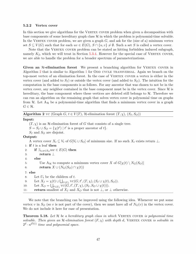
5.2.2 Vertex cover

In this section we give algorithms for the Vertex cover problem when given a decomposition withbase components of some hereditary graph class H in which the problem is polynomial-time solvable.In the Vertex cover problem, we are given a graph G, and ask for the (size of a) minimum vertexset S ⊆ V (G) such that for each uv ∈ E(G), S ∩ u, v 6= ∅. Such a set S is called a vertex cover.

Note that the Vertex cover problem can be stated as hitting forbidden induced subgraph,namely K2, which we will treat in Section 5.3.4. However for the special case of Vertex cover,we are able to handle the problem for a broader spectrum of parameterizations.

Given an H-elimination forest We present a branching algorithm for Vertex cover inAlgorithm 2 that is similar to Algorithm 1 for Odd cycle transversal. Again we branch on thetop-most vertex of an elimination forest. In the case of Vertex cover a vertex is either in thevertex cover (and added to SI) or outside the vertex cover (and added to SO). The intuition for thecomputation in the base components is as follows. For any ancestor that was chosen to not be in thevertex cover, any neighbor contained in the base component must be in the vertex cover. Since H ishereditary, the base component where these vertices are deleted still belongs to H. Therefore wecan run an algorithm on the remaining graph that solves vertex cover in polynomial time on graphsfrom H. Let AH be a polynomial-time algorithm that finds a minimum vertex cover in a graphG ∈ H.

Algorithm 2 vc (Graph G, t ∈ V (T ), H-elimination forest (T, χ), (SI , SO))

Input:(T, χ) is an H-elimination forest of G that consists of a single tree.S = SI ∪ SO = χ(t′) | t′ is a proper ancestor of t.SI and SO are disjoint.

Output:A vertex cover Xt ⊆ Vt of G[Vt ∪ SO] of minimum size. If no such Xt exists return ⊥.

1: if t is a leaf then2: if ∃u,w∈SO

uw ∈ E(G) then3: return ⊥4: else5: Use AH to compute a minimum vertex cover X of G[χ(t) \NG(SO)]6: return X ∪ (NG(SO) ∩ χ(t))

7: else8: Let Ut be the children of t.9: Let XI = χ(t) ∪

⋃t′∈Ut

vc(G, t′, (T, χ), (SI ∪ χ(t), SO)).10: Let XO =

⋃t′∈Ut

vc(G, t′, (T, χ), (SI , SO ∪ χ(t))).11: return smallest of XI and XO that is not ⊥, or ⊥ otherwise.

We note that the branching can be improved using the following idea. Whenever we put somevertex v in SO (so v is not part of the cover), then we must have all of NG(v) in the vertex cover.We do not include it here for ease of presentation.

Theorem 5.18. Let H be a hereditary graph class in which Vertex cover is polynomial timesolvable. Then given an H-elimination forest (F, χ) with depth d, Vertex cover is solvable in2d · nO(1) time and polynomial space.

47

Proof. We solve Vertex cover by summing the results of vc(G[VrT ], rT , (T, χT ), (∅, ∅, ∅)) overall trees T in the forest F . Here rT ∈ V (T ) is the root of T , and χT is the function χ restrictedto V (T ). We argue the correctness of Algorithm 2 by induction on height(Tt). Consider a callvc(G, t, (T, χ), (SI , SO)) that satisfies the input requirements.

If height(Tt) = 0, then t is a leaf and G[χ(t)] ∈ H. For any set Yt ⊆ Vt that satisfies the outputrequirements, the set SO must be an independent set. If this is not the case, we correctly return ⊥.Otherwise for Yt to be a vertex cover, every vertex from NG(SO) ∩ χ(t) must be in the vertex cover.Therefore we return the union of NG(SO) ∩ χ(t) and the result of AH(G[χ(t) \NG(SO)]).

Otherwise, if height(Tt) > 0, then t is not a leaf. We branch on the unique vertex in χ(t) tobe either in the vertex cover or not. In each branch, we recursively call the algorithm for eachchild t′ of t. Since height(Tt′) ≤ height(Tt)− 1, by the induction hypothesis these recursive calls arecorrect. Since there is an ancestor descendant relation for every edge in E(G), the union of vertexcovers for in the recursively called subinstances form a vertex cover for the current instance. Sincethis branching is exhaustive, an optimal vertex cover is found in one of the branches if it exists. IfXI = XO = ⊥, then we can return ∞ for the current instance as well.

Finally, we bound the running time and space requirements, by analyzing the recursion treegenerated by the initial calls on each tree T of the forest F . For each node t ∈ V (T ), there areexactly 2depthT (t) recursive calls to Algorithm 2 with t as the second parameter, one for everypartition of the nodes in the bags of ancestors of t into SI and SO. Within one call, we eitherverify that SO is an independent set in O(n2) time and call AH that runs in nO(1) time, or computethe union of the partial results given by other calls in nO(1) time. Hence the total size of therecursion tree is bounded by 2d · |V (F )| and the work per call is polynomial in n. As we store apolynomial amount of information in each call, this yields the desired bounds on running time andspace requirements.

In the algorithm above we assumed we are given some H-elimination forest. One example whereVertex cover is polynomial time solvable, but no H-elimination forest can be computed in FPTtime is the class of perfect graphs, which we prove in Theorem 6.3. For some graph classes H we doknow how to compute such decompositions, which gives the following.

Corollary 5.19. Let H be a graph class such that H ∈ bipartite, chordal, interval or H ischaracterized by a finite family of forbidden induced subgraphs and Vertex cover is polynomial-time solvable on H. Then Vertex cover is FPT parameterized by edH(G). Furthermore it can be

solved in 2edH(G)O(1)nO(1) time using polynomial space.

Proof. It is well known that Vertex cover is polynomial time solvable on bipartite, chordal, andinterval graphs, as these are subclasses of perfect graphs [58]. Let k = edH(G). By Theorem 4.35,

we can compute an H-elimination forest of depth kO(1) in 2kO(1) · nO(1) time and polynomial space,

for each considered class H. The result follows by supplying the computed decomposition toTheorem 5.18.

One example of a hereditary graph class H that satisfies the premises of the theorem is the classof claw-free (induced K1,3-free) graphs. A maximum independent set (and therefore, its complementwhich forms a minimum vertex cover) can be found in polynomial-time in claw-free graphs [88, 105].

Taking the idea of relaxed parameterizations for Vertex cover one step further, one couldeven combine multiple graph classes in which the problem can efficiently be solved. For example,if H is the class of graphs where each connected component is bipartite, or chordal, or claw-free,then Vertex cover is still FPT parameterized by edH. It is easy to see that the decompositionalgorithms can be adapted to work with the combination of these graph classes, while Theorem 5.18

48

directly applies. This leads to even smaller parameter values. Using the H-treewidth counterpart(Theorem 5.20), we also obtain fixed-parameter tractability for the parameterization by twH.

Given a tree H-decomposition Niedermeier [90] gives an algorithm to solve Vertex covergiven a tree decomposition of width d− 1 in time 2d · nO(1) using a standard dynamic programmingapproach. We adapt this algorithm to work with H-decompositions for hereditary graph classes Hin which vertex cover is polynomial time solvable similar to the H-elimination forest case.

Theorem 5.20. Let H be a hereditary graph class on which Vertex cover is polynomial-timesolvable. Vertex cover can be solved in time 2k · nO(1) when given a tree H-decomposition ofwidth k − 1 consisting of nO(1) nodes.

Proof. We adapt the algorithm by Niedermeier [90, Thm. 10.14]. Choose an arbitrary root for thegiven tree H-decomposition (T, χ, L). For t ∈ V (T ), let Tt be the subtree rooted at t. We keep atable for every t ∈ V (T ), with a row for every assignment Ct : χ(t) \ L → 0, 1. For every suchassignment, we store a value mt(Ct) that denotes the number of vertices in a minimum vertex coverV ′ of the graph induced by

⋃t′∈Tt χ(t′) such that V ′ ∩ (χ(t) \ L) = C−1

t (1). That is, we consider

solutions which contain all vertices in C−1t (1) and none of C−1

t (0). Not every assignment leads to asolution: mt(Ct) =∞ if there is some edge uv with Ct(u) = Ct(v) = 0.

We only have to adapt the computation for the leaf nodes t of the decomposition; the updatesteps remain identical as before [90] since χ(t) ∩ L = ∅ for non-leaf nodes t ∈ V (T ).

For a leaf node t and assignment Ct, define the auxiliary graph G′ := G[(χ(t)∩L) \NG(C−1t (0))]

corresponding to the base component without the vertices which are forced to be in the solutionto cover edges incident on C−1

t (0). As the solutions we are asking for contain all of C−1t (1), none

of C−1t (0) and therefore all of NG(C−1

t (0)) ∩ (χ(t) ∩ L), and furthermore have to cover all edgesof G′, the value of mt can be computed as follows:

mt(Ct) =

+∞ if ∃uv ∈ E(G) : u, v ∈ C−1

t (0)

|C−1t (1)|+ |NG(C−1

t (0)) ∩ χ(t) ∩ L|+ minvc(G′) otherwise.

Note that since H is hereditary and G[χ(t) ∩ L] ∈ H, it follows that G′ ∈ H. Therefore we cancompute the size minvc(G′) of a minimum vertex cover in G′ in nO(1) time. The running time of2k · nO(1) follows.

As before, for certain H we can compute tree H-decompositions to arrive at fixed parametertractability results.

Corollary 5.21. Let H be a graph class such that H ∈ bipartite, chordal, interval or H ischaracterized by a finite family of forbidden induced subgraphs and Vertex cover is polynomial-time solvable on H. Then Vertex cover is FPT parameterized by twH(G) and can be solved in

2twH(G)O(1)nO(1) time.

Proof. It is well known that Vertex cover is polynomial time solvable on bipartite, chordal, andinterval graphs, as these are subclasses of perfect graphs [58]. Let k = twH(G). By Theorem 4.35,

we can compute a tree H-decomposition of width kO(1) in time 2kO(1) · nO(1), for each considered

class H. The result follows by supplying the computed decomposition to Theorem 5.20.

49

5.2.3 Hitting forbidden cliques

We say that a graph is K`-free if it does not contain K` as a subgraph, or equivalently, as an inducedsubgraph. In this section we show how to obtain an FPT algorithm for the K`-free deletionproblem where one is given an (K`-free)-elimination forest, for some ` ≥ 2, and the goal is tocompute the (size of a) minimum vertex set S ⊆ V (G) such that G−S is K`-free. Here ` is assumedto be a constant. Note that the Vertex cover problem is equivalent to K2-free deletion.

The fact that K`-free deletion problem has an FPT algorithm parameterized by the depth ofan (K`-free)-elimination forest will follow from the more general Theorem 5.48 on hitting forbiddeninduced subgraphs, but the branching algorithm we present here has the additional feature that itruns in polynomial space. It is similar to Algorithm 2 for Vertex cover, where we branch onthe top-most vertex of an elimination forest. As with Vertex cover, a vertex is either in thesolution (and added to SI), or not in the solution (and added to SO). The key idea is that a cliquecan occur only on a single root-to-leaf path in an elimination forest. The base component mighthave some ancestors in SO that can still be part of some K`. In the case of ` = 2 (Vertex cover),there is only one remaining option to hit each K2, namely to remove each neighbor of SO in thebase component. In general there are can be as many as `− 1 options to consider. Since the basecomponent is K`-free, by Corollary 5.2 it follows that any optimal solution uses at most d verticesfrom the base component, where d is the depth of the (K`-free)-elimination forest.

Consider the K`-free deletion with forbidden vertices (K`-fdfv) problem, where weare given a graph G, a set of undeletable vertices S ⊆ V (G), and integer k, whereas ` is treated asa constant. The task is to output a minimum set X ⊆ V (G) \ S such that G −X has no K` asinduced subgraph and |X| ≤ k, or ⊥ if no such set exists. We can solve this problem by findingan induced K` in O(n`) time, and then branching on the at most ` ways to delete a non-forbiddenvertex to hit this subgraph. If a solution has not been found after branching for k levels deep,return ⊥. Hence we get the following observation; a formal proof follows from the more generalalgorithm of Lemma 5.47 which is presented later.

Observation 5.22. K`-fdfv(G,S, k) is solvable in `k · nO(1) time and polynomial space.

Theorem 5.23. Given a (K`-free)-elimination forest (F, χ) with depth d for some constant ` ≥ 2,K`-free deletion is solvable in (2`)d · nO(1) time and polynomial space.

Proof. We solve K`-free deletion by summing the results of K`-free deletion(G[VrT ], rT ,(T, χT ), (∅, ∅, ∅)) over all trees T in the forest F . Here rT ∈ V (T ) is the root of T , and χT is thefunction χ restricted to V (T ). To see that this correctly solves the problem, note that any optimalsolution takes at most depthT (t′) vertices from χ(t′) for every leaf t′ ∈ V (T ) by Corollary 5.2.We argue the correctness of Algorithm 3 by induction on height(Tt). Consider a call K`-freedeletion(G, t, (T, χ), (SI , SO)) that satisfies the input requirements.

If height(Tt) = 0, then t is a leaf and G[χ(t) ∩ L] is K`-free. If graph G[SO] is not K`-free, then there is no Xt ⊆ Vt that satisfies the output requirements. Otherwise, the problemis equivalent to an instance of K`-free deletion with forbidden vertices for arguments(G[χ(t) ∪ SO], SO,depthT (t)).

In the remaining case height(Tt) > 0, so t is not a leaf. Recall that there is an ancestor-descendantrelation for every edge in E(G). Therefore any clique occurs on a single root-to-leaf path in thedecomposition. We branch on the unique vertex in χ(t) to be either in the solution or not, andrecursively call the algorithm for each child t′ of t. Since height(Tt′) ≤ height(Tt)− 1, these calls arecorrect by the induction hypothesis. Since a clique occurs on a single root to leaf path, the unionof solutions for the recursively called subinstances forms a solution for the current instance. Since

50

Algorithm 3 K`-free deletion (Graph G, t ∈ V (T ), (T, χ), (SI , SO))

Input:(T, χ) is a (K`-free)-elimination forest G that consists of a single tree.S = SI ∪ SO = χ(t′) | t′ is a proper ancestor of t.SI and SO are disjoint.

Output:A K`-free deletion set Xt ⊆ Vt of G[Vt∪SO] of minimum size, such that |Xt∩χ(t′)| ≤ depthT (t′)for each leaf t′ ∈ V (Tt). If no such Xt exists return ⊥.

1: if t is a leaf then2: if G[SO] contains K` as induced subgraph then3: return ⊥4: else5: return K`-fdfv(G[χ(t) ∪ SO], SO, depthT (t))

6: else7: Let Ut be the children of t.8: Let XI = χ(t) ∪

⋃t′∈Ut

K`-free deletion(G, t′, (T, χ), (SI ∪ χ(t), SO)).9: Let XO =

⋃t′∈Ut

K`-free deletion(G, t′, (T, χ), (SI , SO ∪ χ(t))).10: return smallest of XI and XO that is not ⊥, or ⊥ otherwise.

this branching is exhaustive, the minimum size solution occurs on one of them if it exists. If allsubinstances return ⊥, then we can return ⊥ for the current instance as well.

Finally, we bound the running time and space requirements, by analyzing the recursion treegenerated by the initial calls on each tree T of the forest F . For each node t ∈ V (T ), there areexactly 2depthT (t) recursive calls to Algorithm 2 with t as the second parameter, one for everypartition of the nodes in the bags of ancestors of t into SI and SO. Within one call, we either verifythat G[SO] does not contain K` as induced subgraph in nO(`) = nO(1) time and call K`-fdfv thatruns in `depthT (t) · nO(1) time, or compute the union of the partial results given by other calls innO(1) time. Hence the total size of the recursion tree is bounded by 2d · |V (F )| and the work per calltakes at most `d · nO(1) time. Note that K`-fdfv can be solved using polynomial space. Therefore,as we store a polynomial amount of information in each call, this yields the desired bounds onrunning time and space requirements.

Corollary 5.24. For each fixed ` ≥ 2, K`-free deletion is FPT parameterized by k = edK`-free(G).

Furthermore it can be solved in 2O(k3 log k) · nO(1) time using polynomial space.

Proof. Let k = edK`-free(G). By Theorem 4.35, we can compute a (K`-free)-elimination forest ofdepth O(k3 log k) in 2O(k) · nO(1) time and polynomial space. The result follows by supplying thisdecomposition to Theorem 5.23.

5.3 Generic algorithms via A-exhaustive families

5.3.1 A-exhaustive families and boundaried graphs

In this section we introduce the main tools needed to present our most general framework fordynamic programming on tree H-decompositions. We follow the ideas of gluing graphs and finitestate property dating back to the results of Fellows and Langston [42] (cf. [5, 13]).

The following definition formalizes a key idea for the dynamic programming routine: to computea restricted set of partial solutions out of which an optimal solution can always be built.

51

Definition 5.25. Let H be a graph class, let G be a graph, and let A ⊆ V (G). Then we say that afamily S ⊆ 2A of subsets of A is A-exhaustive for H-deletion on G if for every minimum-sizeset S ⊆ V (G) for which G − S ∈ H, there exists SA ∈ S such that for S′ := (S \ A) ∪ SA wehave |S′| ≤ |S| and G− S′ ∈ H.

As a consequence of this definition, if S is A-exhaustive for H-deletion then there exists anoptimal solution S to H-deletion with S ∩A ∈ S.

The notion of A-exhaustive families is similar in spirit to that of q-representative families formatroids, which have been used in recent algorithms working on graph decompositions [46, 76](cf. [32, §12.3]) to trim the set of partial solutions stored by a dynamic program while preservingthe existence of an optimal solution. As the desired outcome of the replacement process in our caseis not defined in terms of independence in a matroid and there is no particular importance of agiven integer q, we use different terminology for our concept of exhaustive families. We reserve thename of a representative family to refer to a set of representatives for each equivalence class in therelation introduced in Definition 5.28.

The following observation shows how A-exhaustive families can be extended to supersets A′ ⊇ Aby brute force. If |A′ \ A| is bounded, the increase in the size of the exhaustive family can becontrolled.

Observation 5.26. Let H be a graph class, let G be a graph, let A ⊆ V (G) and let S ⊆ 2A beA-exhaustive for H-deletion on G. Then for any set A′ ⊇ A, the family S ′ ⊆ 2A

′defined as

follows has size at most |S| · 2|A′\A| and is A′-exhaustive for H-deletion on G:

S ′ := S1 ∪ S∗ | S1 ∈ S ∧ S∗ ⊆ (A′ \A).

A similar brute-force extension can be done when merging exhaustive families for disjointsubsets A1, A2 into a an A-exhaustive family for a common superset A ⊇ A1 ∪A2. We will use thisstep to handle a variation of standard join bags in a tree decomposition.

Lemma 5.27. Let H be a graph class and let G be a graph. Let A1, A2 ⊆ V (G) be disjoint setsand let S1,S2 be A1-exhaustive (respectively, A2-exhaustive) for H-deletion on G. Then for anyset A′ ⊇ A1 ∪ A2, the family S ′ ⊆ 2A

′defined as follows has size at most |S1| · |S2| · 2|A

′\(A1∪A2)|

and is A′-exhaustive for H-deletion on G:

S ′ := S1 ∪ S2 ∪ S∗ | S1 ∈ S1 ∧ S2 ∈ S2 ∧ S∗ ⊆ (A′ \ (A1 ∪A2)).

Proof. The bound on |S ′| is clear from the definition. Consider an arbitrary optimal solution S ⊆V (G) to H-deletion on G; we will show there exists S ∈ S ′ such that (S \A′) ∪ S is an optimalsolution. We use a two-step argument.

Since S1 is A1-exhaustive, there exists S1 ∈ S1 such that S′ := (S \A1) ∪ S1 is again an optimalsolution.

Applying a similar step to S′, as S2 is A2-exhaustive there exists S2 ∈ S2 such that S′′ :=(S′ \A2) ∪ S2 is an optimal solution.

Since A1 and A2 are disjoint, we have S′′∩A1 = S1 and S′′∩A2 = S2. Let S∗ := S′′∩ (A′ \ (A1∪A2)). It follows that the set S = S1∪S2∪S∗ belongs to S ′. Now note that S\A′ = S′′\A′ as we haveonly replaced parts of the solution within A1 and A2, while A′ ⊇ A1 ∪A2. Hence (S \A′) ∪ S = S′′

is an optimal solution, which concludes the proof.

Note that Lemma 5.27 implies Observation 5.26 by letting A2 = ∅, S2 = ∅.

52

Boundaried graphs For a function f : A → B and a set A′ ⊆ A, we denote by f|A′ : A′ → B

the restriction of f to A′. A k-boundaried graph is a triple G = (G,X, λ), where G is a graph,X ⊆ V (G), and λ : [k] → X is a bijection. We define V (G) = V (G). Two k-boundaried graphs(G1, X1, λ1), (G2, X2, λ2) are compatible if λ2 λ−1

1 is a graph isomorphism between G1[X1] andG2[X2]. Two k-boundaried graphs (G1, X1, λ1), (G2, X2, λ2) are isomorphic if there is a graphisomorphism π : V (G1) → V (G2), such that π|X1

= λ2 λ−11 . The gluing operation ⊕ takes two

compatible k-boundaried graphs (G1, X1, λ1), (G2, X2, λ2), creates their disjoint union, and thenidentifies the vertices λ1[i], λ2[i] for each i ∈ [k]. A tri-separation (A,X,B) of order k in graphG can be naturally decomposed as (G[A ∪X], X, λ)⊕ (G[B ∪X], X, λ) for an arbitrary bijectionλ : [|X|]→ X.

Definition 5.28. We say that two k-boundaried graphs (G1, X1, λ1), (G2, X2, λ2) are (H, k)-equivalent if they are compatible and for every compatible k-boundaried graph (G3, X3, λ3), itholds that (G1, X1, λ1)⊕ (G3, X3, λ3) ∈ H ⇐⇒ (G2, X2, λ2)⊕ (G3, X3, λ3) ∈ H.

Observe that if (G1, X1, λ1) and (G2, X2, λ2) are compatible and G1 and G2 do not belong to H,they are (H, k)-equivalent because we only consider hereditary classes of graphs. Therefore in eachequivalence class of compatibility there can be only one (H, k)-equivalence class that is comprisedof k-boundaried graphs which do not belong to H.

The relevance of the (H, k)-equivalence relation for solving H-deletion can be seen from theobservation below.

Observation 5.29. Consider k-boundaried graphs (G1, X1, λ1), (G2, X2, λ2), (H,X3, λ3), such that(G1, X1, λ1) and (G2, X2, λ2) are (H, k)-equivalent. Let S ⊆ V (H) \X3. Then (H − S,X3, λ3) ⊕(G1, X1, λ1) ∈ H if and only if (H − S,X3, λ3)⊕ (G2, X2, λ2) ∈ H.

The H-membership problem is the problem of deciding whether a given graph belongs to H. Wesay that the H-membership problem is finite state if the relation of (H, k)-equivalence has finitelymany equivalence classes for each k. A k-boundaried graph is called a minimal representative in therelation of (H, k)-equivalence if there is no other k-boundaried graph, which is (H, k)-equivalentand has a smaller number of vertices. A family RHk is called (H, k)-representative if it is comprisedof minimal representatives from all (H, k)-equivalence classes. It will not matter how the ties arebroken. A family RH≤k is called (H,≤ k)-representative if it is a union of (H, t)-representative

families for all t ∈ [k]. We define vol(RH≤k) =∑

R∈RH≤k|V (R)|. Note that even though there may be

many ways to construct such a family, the sum above is well-defined, as well as the size of the family.Let us note that we can effectively test (H, k)-equivalence as long as some (H, k)-representativefamily is known.

Observation 5.30. Let RHk be an (H, k)-representative family. Suppose that k-boundaried graphs(G1, X1, λ1), (G2, X2, λ2) are compatible and for every compatible k-boundaried graph (G3, X3, λ3)from RHk it holds that (G1, X1, λ1)⊕ (G3, X3, λ3) ∈ H ⇐⇒ (G2, X2, λ2)⊕ (G3, X3, λ3) ∈ H. Then(G1, X1, λ1), (G2, X2, λ2) are (H, k)-equivalent.

We will be interested in upper bounding the maximal number of vertices of a graph in an (H,≤ k)-representative familyRH≤k; we will denote this quantity by rH(k). Since there are 2O((rH(k))2) different

graphs on rH(k) vertices, this gives an immediate bound on |RH≤k| and vol(RH≤k). What is more,we can construct an (H,≤ k)-representative family within the same running time.

53

Lemma 5.31. Consider a polynomially recognizable graph class H such that H-membership isfinite state and there is a time-constructible4 function r(k) ≥ k, such that for every integer k and forevery t-boundaried graph, where t ∈ [k], there exists an (H, t)-equivalent t-boundaried graph on atmost r(k) vertices. Then there exists an algorithm that, given an integer k, runs in time 2O((r(k))2)

and returns an (H,≤ k)-representative family.

Proof. Consider a process in which we begin from an empty graph on n vertices, fix t boundaryvertices, and choose an adjacency matrix determining which pairs of vertices share an edge. Byiterating over all possible adjacency matrices, we can generate all t-boundaried graphs on n vertices.

We enumerate all 2O((r(k))2) t-boundaried graphs on at most r(k) vertices, for all t ∈ [k]. Foreach pair of t-boundaried graphs which are compatible, we perform gluing and check (in timepolynomial in r(k)) whether the obtained graph belongs to H. By Observation 5.30, this providessufficient information to divide the generated t-boundaried graphs into (H, t)-equivalence classes. Weconstruct an (H, t)-representative family RHt , for each t ∈ [k], by picking any minimal representativefrom each class; as noted before, it does not matter how the ties are broken.

5.3.2 Dynamic programming with A-exhaustive families

We move on to designing a meta-algorithm for solving H-deletion parameterized by H-treewidth.Let S be an optimal solution and t be a node in a tree H-decomposition. We will associate sometri-separation (A,X,B) with t, where A stands for the set of vertices introduced below t and |X| ≤ kfor k being the width of the decomposition. The main idea is to consider all potential tri-separations(AS , XS , BS) that may be obtained after removing S. We enumerate all the non-equivalent k-boundaried graphs which may be isomorphic with (G[BS ∪XS ], XS) and seek a minimal deletion setwithin A so that the resulting graph belongs to H. We will show that it suffices to consider all therepresentatives in the relation of (H, k)-equivalence to construct an A-exhaustive family of partialsolutions. We shall use the following problem to describe a subroutine for finding such deletion setsin the leaves of the decomposition.

H-deletion with undeletable vertices Parameter: kInput: A graph G, a subset X ⊆ V (G), and an integer k.Task: Either return a minimum-size H-deletion set S ⊆ V (G) \X or conclude that no such setof size at most k exists.

Note that the problem above is equivalent to the H-deletion problem parameterized by thesolution size k where no vertices are undeletable. The following lemma shows that the requirementof having undeletable vertices is easy to overcome if H is closed under the addition of true twins.We say that vertices u, v ∈ V (G) are true-twins if NG[u] = NG[v].

Lemma 5.32. Let H be a graph class closed under the addition of true twins and such that H-deletion parameterized by the solution size k can be solved in f(n, k) time. Then the problemH-deletion with undeletable vertices can be solved in f(k · n, k) time.

Proof. Let G′ be the graph obtained from G by making k + 1 new true-twin copies of every vertexin the undeletable set X. Then for every set S ⊆ V (G) \X for which G − S is a member of H,the graph G′ − S is also in H. Conversely, any minimum-size set S ⊆ V (G′) of size at most kfor which G′ − S in H does not contain any copies of vertices in X, as the budget of k vertices isinsufficient to contain all copies of a vertex, while a solution that avoids one copy of a vertex can

4A function r : N→ N is time-constructible if there exists a Turing machine that, given a string 1k, outputs thebinary representation of r(k) in time O(r(k)). We add this condition so we can assume that the value of r(k) is knownto the algorithm. All functions of the form r(k) = α · kc, where α, c are positive integers, are time-constructible.

54

avoid all copies, since members of H are closed under the addition of true twins. Consequently, anoptimal solution in G′ of size at most k is disjoint from X, and is also a solution in the inducedsubgraph G of G′. Hence to compute a set S as desired, it suffices to compute an optimal chordaldeletion set in G′ if there is one of size at most k, which can be done by assumption.

Lemma 5.33. Suppose that H-membership is finite state, H is closed under disjoint union of graphs,and H-deletion with undeletable vertices admits an algorithm with running time f(k) ·nO(1).Then there is an algorithm that, given a tri-separation (A,X,B) of order k in a graph G such thatG[A] ∈ H, and an (H,≤ k)-representative family RH≤k, runs in time 2k · f(k) · vol(RH≤k)O(1) · nO(1)

and outputs a family S of size at most 2k · |RH≤k| that is A-exhaustive for H-deletion on G.

Proof. Initialize S = ∅. For each subset X ′ ⊆ X, fix an arbitrary bijection λ : [|X ′|] → X ′ andconsider the graph G − (X \X ′). It admits a tri-separation (A,X ′, B). For each representativeR ∈ RHt , where t = |X ′|, which is compatible with (G[B∪X ′], X ′, λ), we perform the gluing operationGR = (G[A ∪ X ′], X ′, λ) ⊕ R and execute the algorithm for H-deletion with undeletablevertices on GR with the set of undeletable vertices V (GR) \A and parameter k. That is, we seekfor a minimum-size deletion set A′ ⊆ A of size at most k. If such a set is found, we add it to S.

The constructed family clearly has size at most 2k · |RH≤k|. The running time can be upper

bounded by 2k ·∑

R∈RH≤kf(k)(n+ |V (R)|)O(1) = 2k · f(k) · vol(RH≤k)O(1) · nO(1). It remains to show

that S is indeed A-exhaustive.Consider a minimum-size solution S to H-deletion on G. Define SA, SX , SB as S ∩ A,S ∩

X,S ∩B, respectively, and let X ′ := X \SX , |X ′| = t. Fix an arbitrary bijection λ : [t]→ X ′. SinceH is closed under disjoint union of graphs and G[A] ∈ H, by Lemma 5.1 we know that |SA| ≤ k.The set RHt contains a t-boundaried graph R that is (H, t)-equivalent to (G[B ∪X ′]− SB, X ′, λ).By Observation 5.29, SA is an H-deletion set for (G[A ∪X ′], X ′, λ)⊕R. As (G[A ∪X ′], X ′, λ)⊕Rcontains an H-deletion set within A of size at most k, some set S′A with this property has been addedto S. Furthermore, S′A is a minimum-size solution, so |S′A| ≤ |SA|. Again by Observation 5.29, S′A isan H-deletion set for (G[A∪X ′], X ′, λ)⊕ (G[B∪X ′]−SB, X ′, λ). It means that S′ = (S \A)∪S′A =SB ∪ SX ∪ S′A is an H-deletion set in G and |S′| ≤ |S|, which finishes the proof.

The next step is to propagate the partial solutions along the decomposition in a bottom-upmanner. As we want to grow the sets A for which A-exhaustive families are computed, we can takeadvantage of Observation 5.26 and Lemma 5.27. However, after processing several nodes, the size ofA-exhaustive families computed this way can become arbitrarily large. In order to circumvent this,we shall prune the A-exhaustive families after each step.

Lemma 5.34. Suppose that H-membership is finite state and graphs in the class H can berecognized in polynomial time. There is an algorithm that, given a tri-separation (A,X,B) of order kin a graph G, a family S ′ ⊆ 2A that is A-exhaustive for H-deletion on G, and an (H,≤ k)-representative family RH≤k, runs in time 2k · |S ′| · vol(RH≤k)O(1) · nO(1) and outputs a family S ⊆ S ′

of size at most 2k · |RH≤k| that is A-exhaustive for H-deletion on G.

Proof. Initialize S = ∅. For each subset X ′ ⊆ X, fix an arbitrary bijection λ : [|X ′|] → X ′ andconsider the graph G− (X \X ′). It admits a tri-separation (A,X ′, B). For each graph R ∈ RHt ,where t = |X ′|, which is compatible with (G[B ∪ X ′], X ′, λ), we perform the gluing operationGR = (G[A ∪ X ′], X ′, λ) ⊕ R. Using the polynomial-time recognition algorithm we choose aminimum-size set SA ∈ S ′ which is an H-deletion set for GR, if one exists, and add it to S.

55

We construct at most 2k · |RH≤k| graphs GR. For each graph GR we add at most one set to S and

spend |S ′|·(n+|R|)O(1) time. In total, we perform at most 2k ·|RH≤k|·|S ′|·∑

R∈RH≤k(n+|V (R)|)O(1) =

2k · |S ′| · vol(RH≤k)O(1) · nO(1) operations. It remains to show that S is indeed A-exhaustive.Consider a minimum-size solution S to H-deletion on G. Define SA, SX , SB as S∩A,S∩X,S∩

B, respectively, and let X ′ := X \ SX , |X ′| = t. Since S ′ is A-exhaustive on G, there exists SA ∈ S ′such that S = (S \ A) ∪ SA is also a minimum-size solution to G, implying that |SA| ≤ |SA|.Fix an arbitrary bijection λ : [t] → X ′. The set RHt contains a t-boundaried graph R that is(H, t)-equivalent to (G[B ∪X ′] − SB, X ′, λ). By Observation 5.29, a set A′ ⊆ A is an H-deletionset for G′ = (G[A ∪X ′], X ′, λ)⊕ (G[B ∪X ′]− SB, X ′, λ) if and only if A′ is an H-deletion set for(G[A ∪X ′], X ′, λ) ⊕ R. Since G′ − SA = G − S ∈ H, we know that SA ∈ S ′ is such a set. Henceby the construction above, there exists some (possibly different) S′A ∈ S with this property and

minimum size; hence |S′A| ≤ |SA| ≤ |SA| and S′ = (S \ A) ∪ S′A = SB ∪ SX ∪ S′A is an H-deletionset in G and |S′| ≤ |S|. The claim follows.

We are ready to combine the presented subroutines in a general meta-algorithm to process treeH-decompositions for every class H which satisfies three simple conditions. The following statementformalizes and, together with Lemma 5.31, proves Theorem 2.1 from Section 2.2.

Theorem 5.35. Suppose that the class H satisfies the following:

1. H is hereditary and union-closed,

2. H-deletion with undeletable vertices admits an algorithm with running time f(k′) ·nO(1), where k′ is the parameter,

3. H-membership is finite state and there is an algorithm computing an (H,≤ k′′)-representativefamily with running time v(k′′).

Then H-deletion can be solved in time 2O(k)·f(k)·v(k)O(1)·nO(1) when given a tree H-decompositionof width k − 1 consisting of nO(1) nodes.

Proof. First, we construct an (H,≤ k)-representative family RH≤k in time v(k). Since the output

size of the algorithm cannot exceed its running time, we have |RH≤k| ≤ vol(RH≤k) ≤ v(k).The algorithm is based on a variant of dynamic programming in which bounded-size sets of

partial solutions are computed, with the guarantee that at least one of the partial solutions whichare stored can be completed to an optimal solution. More formally, for each node t ∈ V (T ) weare going to compute (recall κ, π from Definition 5.7) a set of partial solutions St ⊆ 2κ(t) of sizeat most 2k · |RH≤k| which is κ(t)-exhaustive for H-deletion in G. As κ(r) = V (G) for the rootnode r by Observation 5.8, any minimum-size set S ∈ Sr for which G−S ∈ H is an optimal solutionto the problem, and the property of κ(r)-exhaustive families guarantees that one exists. We dothe computation bottom-up in the tree decomposition, using Lemma 5.34 to prune sets of partialsolutions at intermediate steps to prevent them from becoming too large.

Let (T, χ, L) be a tree H-decomposition of width k − 1. By Lemma 5.5 we may assume that thedecomposition is nice and is rooted at some node r. For t ∈ V (T ), define Lt := L∩χ(t). Process thenodes of T from bottom to top. We process a node t after having computed exhaustive families forall its children, as follows. Let Xt := χ(t) ∩ π(t), let At := κ(t) and let Bt := V (G) \ (At ∪Xt). ByObservation 5.9, the partition (At, Xt, Bt) is a tri-separation of G. The way in which we continueprocessing t depends on the number of children it has. As T is a nice decomposition, node t has atmost two children.

56

Leaf nodes For a leaf node t ∈ V (T ), we construct a exhaustive family of partial solutions St ⊆2κ(t) as follows. By Definition 3.4, vertices of Lt do not occur in other bags than χ(t). Because thedecomposition is nice, we have χ(t) \ Lt = π(t). Therefore κ(t) = Lt and we have (At, Xt, Bt) =(Lt, χ(t) \ Lt, V (G) \ χ(t)). Furthermore, |Xt| ≤ k since the width of the decomposition is k − 1.As G[Lt] ∈ H, we can process the tri-separation (At, Xt, Bt) with Lemma 5.33 within running time2k · f(k) · v(k)O(1) · nO(1). We obtain a κ(t)-exhaustive family of size at most 2k · |RH≤k|.

Nodes with a unique child Let t be a node that has a unique child c, for which a κ(c)-exhaustive family Sc of size 2k · |RH≤k| has already been computed. Recall that vertices of L onlyoccur in leaf bags, so that Lt = ∅ and therefore |χ(t)| ≤ k. Observe that κ(t) \ κ(c) ⊆ χ(t), sothat |κ(t) \ κ(c)| ≤ k. Compute the following set of partial solutions:

S ′t := Sc ∪ S∗ | Sc ∈ Sc, S∗ ⊆ κ(t) \ κ(c).

Since the number of choices for Sc is 2k · |RH≤k|, while the number of choices for S∗ is 2k, the set S ′thas size at most 22k · |RH≤k| and can be computed in time 22k · |RH≤k| · nO(1). Since κ(c) ⊆ κ(t) dueto Observation 5.8, we can invoke Observation 5.26 to deduce that the family S ′t is κ(t)-exhaustivefor H-deletion on G. As the last step for the computation of this node, we compute the desiredexhaustive family St as the result of applying Lemma 5.34 to S ′t and the tri-separation (At, Xt, Bt)of G, which is done in time 23k · v(k)O(1) · nO(1) because |RH≤k| ≤ v(k). As At = κ(t), the lemmaguarantees that St is κ(t)-exhaustive and it is sufficiently small.

Nodes with two children The last type of nodes to handle are those with exactly twochildren. So let t ∈ V (T ) have two children c1, c2. Since t is not a leaf we have Lt = ∅. Let K :=κ(t) \ (κ(c1) ∪ κ(c2)) and observe that K ⊆ χ(t) \ L. Therefore |K| ≤ k.

Using the κ(c1)-exhaustive set Sc1 and the κ(c2)-exhaustive set Sc2 computed earlier in thebottom-up process, we define a set S ′t as follows:

S ′t := S1 ∪ S2 ∪ S∗ | S1 ∈ Sc1 , S2 ∈ Sc2 , S∗ ⊆ K.

As Sc1 and Sc2 both have size 2k · |RH≤k|, while |K| ≤ 2k, we have |S ′t| = 23k · |RH≤k|2. ByObservation 5.8 we have that κ(c1)∩κ(c2) = ∅ and κ(c1)∪κ(c2) ⊆ κ(t), so we can apply Lemma 5.27to obtain that the family S ′t is κ(t)-exhaustive for H-deletion on G. The desired exhaustivefamily St is obtained by applying Lemma 5.34 to S ′t and the tri-separation (At, Xt, Bt) of G, whichis done in time 24k · v(k)O(1) · nO(1)

Wrapping up Using the steps described above we can compute, for each node of t ∈ V (T ) in abottom-up fashion, a κ(t)-exhaustive family St of size 2k · |RH≤k|. Since the number of nodes of t

is nO(1) the overall running time follows. As discussed in the beginning of the proof, an optimalsolution can be found by taking any minimum-size solution from the family Sr for the root r.

5.3.3 Hitting forbidden connected minors

As a first application of the meta-theorem, we consider classes defined by a finite set of forbiddenconnected minors. The seminal results of Robertson and Seymour [101] state that every minor-closedfamily H can be defined by a finite set of forbidden minors. The H-deletion problem is FPT forsuch classes when parameterized by the solution size [1, 103] or by treewidth [7]. The requirementthat all the forbidden minors are connected holds whenever H = D(H), that is, H is closed undertaking disjoint union of graphs. In Section 6.2 we argue why this limitation is necessary.

Unlike the next sections, here we do not need to prove any claims about structure of minor-closedclasses and we can just take advantage of known results in a black-box manner. In order to applyTheorem 5.35, we first need to bound the sizes of representatives in RHk . To this end, we shall take

57

advantage of the recent result of Baste, Sau, and Thilikos [6], who have studied optimal runningtimes for H-deletion parameterized by treewidth. They define a relation of (≤ h, k)-equivalence:two k-boundaried graphs (G1, X1, λ1), (G2, X2, λ2) are (≤ h, k)-equivalent if they are compatible andfor every graph F on at most h vertices and for every compatible k-boundaried graph (G3, X3, λ3),F is a minor of (G1, X1, λ1)⊕ (G3, X3, λ3) if and only if F is a minor of (G2, X2, λ2)⊕ (G3, X3, λ3).

Theorem 5.36 ([6, Thm. 6.2]). There is a computable function f , so that if (R,X, λ) is a k-boundaried graph and R is Kq-minor-free, then there exists a k-boundaried graph (R′, X ′, λ′) whichis (≤ h, k)-equivalent to (R,X, λ) and |V (R′)| ≤ f(q, h) · k.

Let H be a class defined by a family of forbidden minors, which are all connected and haveat most h vertices. Then whenever two k-boundaried graphs are (≤ h, k)-equivalent, they arealso (H, k)-equivalent. Moreover, if Kh is a minor of R, then (R,X, λ) is (H, k)-equivalent to anycompatible k-boundaried graph which contains Kh as a minor. In particular, one can always findsuch a graph on at most k + h vertices. This leads to the following corollary.

Corollary 5.37. Let H be a class defined by a finite family of forbidden minors. There exists aconstant dH such that for every minimal representative R in the relation of (H, k)-equivalence wehave |V (R)| ≤ dH · k.

Lemma 5.38. Let H be a class defined by a finite non-empty family of forbidden minors. There existsan algorithm that, given an integer k, runs in time 2O(k log k) and returns an (H,≤ k)-representativefamily.

Proof. We take advantage of the fact that graphs in H are sparse, that is, there exists a constantcH such that if G ∈ H then |E(G)| ≤ cH · |V (G)| [84]. Any graph G ∈ H on n vertices can berepresented by a set of at most cH · n pairs of vertices which share an edge. Therefore the numberof such graphs is 2O(n logn).

We proceed similarly as in Lemma 5.31 by generating all 2O(k log k) t-boundaried graphs on atmost dH · k vertices (see Corollary 5.37), whose underlying graph belong to H, for all t ∈ [k]. Foreach pair of t-boundaried graphs which are compatible, we perform gluing and check whether theobtained graph belongs to H. Then by Observation 5.30 it suffices to pick any minimal representativefrom each computed equivalence class, and add a single t-boundaried graph with a forbidden minorfor each t ∈ [k].

Furthermore, it turns out that the known algorithms for H-deletion parameterized by thesolution size can be adapted to work with undeletable vertices.

Theorem 5.39 ([103]5). Let H be a class defined by a finite family of forbidden minors. Then

H-deletion with undeletable vertices admits an algorithm with running time 2kO(1) · n3,

parameterized by the solution size k.

In order to obtain a better final guarantee for the most important case H = planar, we needa concrete bound on the exponent in the running time for H-deletion with undeletablevertices. The fastest known algorithm for Planar deletion is due to Jansen, Lokshtanov, andSaurabh [68] and runs in time 2O(k log k) · n, but it is not clear whether it can be adapted to workwith undeletable vertices. We shall therefore rely on the algorithm by Kociumaka and Pilipczukwith a slightly worse running time, which can be extended to support integer weights on vertices [75,§6]. By setting the weight of each undeletable vertex to k + 1 and 1 for other vertices, we arrive atthe following conclusion.

5The details can be found in the full version of the article [104, Section 8].

58

Theorem 5.40 ([75]). Planar deletion with undeletable vertices admits an algorithmwith running time 2O(k2 log k) · nO(1), parameterized by the solution size k.

We are ready to combine all the ingredients and apply the meta-theorem. Note that the bottle-neck of the obtained running time comes from solving the subproblem with undeletable verticeswhereas computing exhaustive families in an internal node takes time 2O(k log k). This means thatLemma 5.38 does not lead to any improvement over the naive approach from Lemma 5.31 in the finalrunning time. Nevertheless, we have prepared our framework for the possibility that the runningtime of the form 2O(k log k) · nO(1) for Planar deletion with undeletable vertices is obtainedin the future, so that the case H = planar could be improved.

Theorem 5.41. Let H be a class defined by a finite family of forbidden connected minors. ThenH-deletion can be solved in time 2k

O(1) · nO(1) when given a tree H-decomposition of width k − 1consisting of nO(1) nodes. In the special case of H = planar the running time is 2O(k2 log k) · nO(1).

Proof. We check the conditions of Theorem 5.35. The class H is hereditary and closed under disjointunion of graphs because the forbidden minors are connected. By Theorem 5.39, H-deletion withundeletable vertices can be solved in time 2k

O(1) · n3 and by Theorem 5.40, Planar deletionwith undeletable vertices can be solved in time 2O(k2 log k) · n. Finally, by Lemma 5.38 there isan algorithm computing an (H,≤ k)-representative family in time v(k) = 2O(k log k).

Finally, we invoke the algorithm for computing a tree H-decomposition of approximate width toinfer the general tractability result.

Corollary 5.42. Let H be a class defined by a finite family of forbidden connected minors. ThenH-deletion can be solved in time 2k

O(1) ·nO(1) where k = twH(G). In the special case of H = planarthe running time is 2O(k10 log k) · nO(1).

Proof. By Theorem 4.35 we can find a tree H-decomposition of width O((twH(G))5

)in time

2kO(1) · nO(1). For H = planar the running time guarantee is 2O(k2 log k) · nO(1). It remains to apply

Theorem 5.41 with parameter k′ = O((twH(G))5

).

5.3.4 Hitting forbidden connected induced subgraphs

In this section we deal with graph classes H defined by a finite family F of forbidden inducedsubgraphs. The problem of hitting finite forbidden (induced) subgraphs, parameterized by treewidth,has been studied by several authors [33, 94, 102].

We introduce some terminology for working with induced subgraphs and isomorphisms. Forgraphs G and H, a function f : V (H)→ V (G) is an induced subgraph isomorphism from H to G if fis injective and satisfies xy ∈ E(H)⇔ f(x)f(y) ∈ E(G) for all x, y ∈ V (H). A function f ′ : A→ Bis an extension of a function f : A′ → B if f ′|A′ = f .

Definition 5.43. Let F be a finite family of graphs. The operation of F-pruning a k-boundariedgraph (G,X, λ) is defined as follows:

• Initialize all vertices of V (G) \X as unmarked.

• For each F ∈ F , for each tri-separation (AF , XF , BF ) of H with BF 6= ∅, for each inducedsubgraph isomorphism f from H[XF ] to G[XG], if there exists an induced subgraph isomorphismfrom H[XF ∪BF ] to G that is an extension of f , then mark the vertex set f ′(b) | b ∈ BF for one such extension f ′, chosen arbitrarily.

59

• Remove all vertices of V (G) \X which are not marked at the end of the process.

Observe that graph resulting from the operation of F-pruning depends on the choices madefor f ′. Our statements and algorithms are valid regardless how these ties are broken as long as thegraphs produced by F -pruning two isomorphic graphs are also isomorphic. We remark that there isno need to consider implementation aspects of F-pruning because we only use it for an existentialbound on the sizes of representatives.

Lemma 5.44. Let H be a class defined by a finite family F of forbidden induced subgraphs.Let (G1, X, λ) be a k-boundaried graph and suppose that (G2, X, λ) was obtained by F-pruning (G1, X, λ).Then (G1, X, λ) and (G2, X, λ) are (H, k)-equivalent.

Proof. First observe that these graphs are compatible because F -pruning removes a subset of verticesfrom V (G1) \X. As G2 is an induced subgraph of G1, the forward implication of Definition 5.28 istrivial. We prove that for any compatible k-boundaried graph H it holds that if H ⊕ (G2, X, λ) isinduced-F-free, then also H ⊕ (G1, X, λ) is induced-F-free.

Assume for a contradiction that G = H ⊕ (G1, X, λ) contains an induced subgraph isomorphicto F for some F ∈ F . Let (A,X,B) be the tri-separation of G, so that (G[A ∪ X], X, λ) isisomorphic with H and (G[B ∪X], X, λ) is isomorphic with (G1, X, λ). Let B′ ⊆ B be the set ofvertices marked during F-pruning (G[B ∪X], X, λ). Let f be an induced subgraph isomorphismfrom F to G. We define a tri-separation of F based on f : let AF := v ∈ V (F ) | f(v) ∈ A,let XF := v ∈ V (F ) | f(v) ∈ X, and let BF := v ∈ V (F ) | f(v) ∈ B. Observe that if BF = ∅,then the image of F is fully contained in A∪X, and so G[A∪X ∪B′] = H ⊕ (G2, X, λ) contains Fas an induced subgraph, which gives a contradiction. Assume from now on that BF 6= ∅.

Note that f|XFis an induced subgraph isomorphism from F [XF ] to G[X] (if XF = ∅ this is an

empty isomorphism, which is also considered during F -pruning), and that f|XF∪BFis an extension

of f|XFthat forms an induced subgraph isomorphism from F [XF ∪BF ] to G[X∪B]. Consequently, in

the process of F -pruning (G[B ∪X], X, λ) we considered F , the function f|XF, and an extension f ′

of f|XFthat is an induced subgraph isomorphism from F [XF ∪ BF ] to G[X ∪ B]. Hence the

vertices f ′(b) | b ∈ BF were marked during the pruning process and are preserved in B′. It followsthat f ′ is also an induced subgraph isomorphism from F [XF ∪ BF ] to G[X ∪ B′]. Now considerthe function f∗ : V (F )→ V (G) such that f∗|AF∪XF

= f and f∗|BF= f ′, and recall that f|XF

= f ′|XF.

As the tri-separation of G ensures that f(x)f(y) /∈ E(G) for any x ∈ AF and y ∈ BF , it caneasily be verified that f∗ is an induced subgraph isomorphism from F to G[A ∪ X ∪ B′]. Thisgraph is isomorphic with H ⊕ (G2, X, λ), so it also contains an induced subgraph isomorphic to F :a contradiction to the assumption that H ⊕ (G2, X, λ) is induced-F-free.

Since F-pruning preserves the (H, k)-equivalence class, we can assume that the minimal repre-sentatives cannot be reduced by F-pruning. It then suffices to estimate the maximal number ofvertices left after F -pruning. For a graph F on c vertices, there are at most 3c tri-separations of Fas each vertex either belongs to AF , XF , or BF . The number of induced subgraph isomorphismsfrom XF to XG is bounded by kc, where k = |X|, as for each of the at most c vertices in XF thereare at most k options for their image. For each such induced subgraph isomorphism we mark atmost c vertices.

Observation 5.45. Let F be a finite family of graphs on at most c vertices each. The operationof F-pruning a k-boundaried graph (G,X, λ) removes all but |F| · 3c · kc · c vertices from V (G) \X.

Corollary 5.46. Let H be a graph class defined by a finite set F of forbidden induced subgraphs onat most c vertices each. If (R,X, λ) is a minimal representative in the relation of (H, k)-equivalence,then |V (R)| = O(kc).

60

As the next step, we need to provide an algorithm for H-deletion parameterized by the solutionsize, which works with undeletable vertices. This can be done via a straightforward application ofthe technique of bounded-depth search trees.

Lemma 5.47. Let H be a graph class defined by a finite set F of forbidden induced subgraphs onat most c vertices each. Then H-deletion with undeletable vertices admits an algorithmwith running time ck · nO(1).

Proof. Given an input (G, k,X), find an induced subgraph isomorphism f from some H ∈ F to G,if one exists. As c is constant, this can be done in time nO(1) by brute force. If no such f exists, thenoutput the empty set as the optimal solution. Otherwise, let T := f(v) | v ∈ V (H) denote thevertices in the range of f . Any valid solution has to include a vertex of T \X. If k = 0 or T ⊆ X,then clearly no solution of size at most k exists and we report failure. Otherwise, for each of the atmost c vertices v ∈ T \X we recurse on the instance (G− v, k − 1, X). If all recursive calls reportfailure, then we report failure for this call as well. If at least one branch succeeds, then we take aminimum-size solution S′ returned by a recursive call and add v to it to form the output.

Since the branching is exhaustive, it is easy to see that the algorithm is correct. As the depth ofthe recursion tree is at most k, while the algorithm branches on |T \X| ≤ c vertices at every step,the claimed running time follows.

We can now combine all the ingredients and plug them into the meta-theorem. Even though c isconstant, we can keep track of how it affects the exponent at k, as it follows easily from the claimsabove. Observe that so far we never had to assume that the graphs in the family F are connected,but this requirement is crucial for the tractability (see Section 6.2).

Theorem 5.48. Let H be a graph class defined by a finite set F of forbidden induced subgraphs on atmost c vertices each, which are all connected. Then H-deletion can be solved in time 2O(k2c) ·nO(1)

when given a tree H-decomposition of width k − 1 consisting of nO(1) nodes.

Proof. We check the conditions of Theorem 5.35. The class H is hereditary and closed under disjointunion of graphs because the forbidden subgraphs are connected. By Lemma 5.47, H-deletionwith undeletable vertices can be solved in time ck · nO(1). Finally, by Corollary 5.46 andLemma 5.31, an (H,≤ k)-representative family can be computed in time v(k) = 2O(k2c).

Corollary 5.49. For any graph class H which is defined by a finite set F of connected forbiddeninduced subgraphs on at most c vertices each, H-deletion can be solved in time 2O(k6c) ·nO(1) whenparameterized by k = twH(G), and in time 2O(k4c) · nO(1) when parameterized by k = edH(G).

Proof. We use Theorem 4.35 to find a tree H-decomposition of width O(k3), which takes time2O(k) · nO(1), and plug it into Theorem 5.48. To see the second claim, observe that Theorem 4.35allows us to find an H-elimination forest of width O(k2) in time 2O(k2) · nO(1). This gives usa tree H-decomposition of the same width (see Lemma 3.5), which can be again supplied toTheorem 5.48.

5.3.5 Chordal deletion

In this section we develop a dynamic-programming algorithm that solves Chordal deletion usinga tree chordal-decomposition. We again want to use the meta-algorithm presented in Theorem 5.35.To this end, we need to bound the sizes of representatives in the relation of (chordal, k)-equivalence.We obtain it through a new criterion that tests whether a graph G is chordal based on several

61

properties of a tri-separation (A,X,B) in G. We therefore first develop some theory of chordalgraphs.

A hole in a graph G is an induced cycle of length at least four. A graph is chordal if it doesnot contain any holes. We need the following observation, which follows easily from the alternativecharacterization of chordal graphs as intersection graphs of the vertex sets of subtrees of a tree [56].

Observation 5.50. Chordal graphs are closed under edge contractions.

A vertex v in a graph G is simplicial if the set NG(v) forms a clique in G. Since a hole does notcontain any simplicial vertices, we have the following.

Observation 5.51. If v is a simplicial vertex in G, then G is chordal if and only if G−v is chordal.Consequently, if a graph G′ is obtained from a chordal graph G by inserting a new vertex whoseneighborhood is a clique in G, then G′ is chordal.

Lemma 5.52 ([17, Thm. 5.1.1]). Every chordal graph contains a simplicial vertex.

The following structural property of chordal graphs will be used to bound the sizes of represen-tatives, once their structure is revealed.

Lemma 5.53. If G is a chordal graph and A∪B is a partition of V (G) such that B is an independentset in G and no vertex of B is simplicial in G, then |B| < |A|.

Proof. Proof by induction on |A|. If |A| = 1 then B = ∅, as vertices in the independent set B caneither be isolated or adjacent to the unique vertex in A, which would make them simplicial.

For the induction step, let |A| > 1 and let v ∈ V (G) be a simplicial vertex, which exists byLemma 5.52. By the precondition to the lemma, v ∈ A. Let Bv := NG(v) ∩ B. Since Bv is aclique as v is simplicial, while B ⊇ Bv is an independent set by assumption, we have |Bv| ≤ 1.Let G′ := G− (v ∪ Bv). Then the vertices of B \ Bv are not simplicial in G′, as the non-edgesin their neighborhood do not involve v. By inductive assumption the graph G′ with its partitioninto A′ := A \ v and B′ := B \ Bv satisfies |B′| = |B \ Bv| < |A′| = |A| − 1. As |Bv| ≤ 1, thisimplies the lemma.

Recall that a walk from a vertex u to a vertex v in a graph G is a sequence of (not necessarilydistinct) vertices, starting with u and ending with v, such that consecutive vertices are adjacentin G. The vertices u and v are the endpoints of the walk; all other vertices occurring on the walk areinternal vertices. The following observation gives an easy way to certify that a graph is not chordal.

Observation 5.54 ([86, Proposition 3]). If a graph G contains a vertex v with two nonadjacentneighbors u1, u2 ∈ NG(v), and a walk from u1 to u2 with all internal vertices in V (G) \NG[v], thenG contains a hole passing through v.

We are ready to formulate an operation used to produce representatives of bounded size.

Definition 5.55. Let (G,X, λ) be a k-boundaried graph. The operation of condensing (G,X, λ) isdefined as follows.

• For each connected component Bi of G−X for which G[NG(Bi)] is a clique, called a simplicialcomponent, remove all vertices of Bi.

• For each connected component Bi of G −X for which G[NG(Bi))] is not a clique, called anon-simplicial component, contract Bi to a single vertex.

62

We want to show that condensing boundaried graphs preserves its equivalence class. To thisend, we show that we can harmlessly contract any edge which is not incident with the separator X.

Lemma 5.56. Let G be a graph, (A,X,B) be a tri-separation in G, and let u, v ∈ B, uv ∈ E(G).Then G is chordal if and only if the following conditions hold:

1. The graphs G[A ∪X] and G[B ∪X] are chordal.

2. The graph G/uv is chordal.

Proof. If G is chordal, then since chordal graphs are hereditary and closed under edge contractionsby Observation 5.50, both conditions are satisfied.

We prove the reverse implication. Suppose that G[A ∪X], G[B ∪X] and G/uv are chordal butG is not, that is, it contains a hole H. As both G[A∪X] and G[B ∪X] are chordal, hole H containssome a ∈ A and some b ∈ B.

Consider a vertex a ∈ A that lies on hole H, and let p, q be the predecessor and successorof a on the hole. Then p, q ∈ NG(a) and therefore p, q /∈ B by the properties of a tri-separation.Furthermore, pq /∈ E(G) since a hole is chordless. The subgraph P := H − a forms an inducedpath between p and q in G. Since u, v ∈ B and a ∈ A, we have u, v /∈ NG(a). As contractionspreserve the connectivity of subgraphs, when contracting edge uv the path P turns into a (possiblynon-simple) walk between nonadjacent p, q ∈ NG(a) in G/uv, whose internal vertices avoid NG[a]since neither of the contracted vertices is adjacent to a. By Observation 5.54, this implies G/uvcontains a hole; a contradiction.

Lemma 5.57. Let (G1, X, λ) be a k-boundaried graph, so that G1 is chordal, and let (G2, X, λ) beobtained by condensing (G1, X, λ). Then (G1, X, λ) and (G2, X, λ) are (chordal, k)-equivalent.

Proof. The condensing operation does not affect the boundary X so these graphs are compatible.Since G1 is chordal, the same holds for G2 because chordal graphs are closed under contractingedges and removing vertices. Consider a k-boundaried graph H compatible with (G1, X, λ). By thesame argument as above, if H ⊕ (G1, X, λ) is chordal, then H ⊕ (G2, X, λ) is as well.

We now prove the second implication. Suppose that H ⊕ (G2, X, λ) is chordal, so the underlyinggraph in H is chordal as well. Let (A,X,B) be a tri-separation of G = H ⊕ (G1, X, λ), so that(G[A ∪X], X, λ) is isomorphic with H and (G[B ∪X], X, λ) is isomorphic with (G1, X, λ). By thedefinition of condensing, H ⊕ (G2, X, λ) can be obtained from G by contracting each connectedcomponent of G[B] to a single vertex – let us refer to this graph as G′ – and then removing somesimplicial vertices. Since G′ can be obtained from the chordal graph H ⊕ (G2, X, λ) by insertingsimplicial vertices, then G′ is chordal by Observation 5.51. Let G = G1, G2, . . . , Gm = G′ be thegraphs given by the series of edge contractions that transforms G into G′. We prove that if Gi+1 ischordal, then Gi is as well. The graph Gi admits a tri-separation (A,X,Bi), so that Gi[Bi ∪X] isobtained from G[B ∪X] via edge contractions, therefore Gi[Bi ∪X] is chordal. Moreover, Gi[A∪X]is isomorphic with the underlying graph in H, so it is also chordal, and Gi+1 is obtained from Gi bycontracting an edge in Bi. We can thus apply Lemma 5.56 to infer that Gi is chordal. It followsthat G = H ⊕ (G1, X, λ) is chordal, which finishes the proof.

Corollary 5.58. If (R,X, λ) is a minimal representative in the relation of (chordal, k)-equivalence,then |V (R)| ≤ 2k + 4.

Proof. By Lemma 5.57 we obtain that condensing preserves (chordal, k)-equivalence. If (R,X, λ) isa minimal-size representative and R is chordal, it must be condensed. Therefore V (R) \X is anindependent set and no v ∈ V (R) \X is simplicial. From Lemma 5.53 we get that |V (R) \X| < |X|

63

and therefore |V (R)| ≤ 2k−1. If R is not chordal, then it is (chordal, k)-equivalent to any compatiblek-boundaried graph, which is not chordal. One can always find such a graph on k + 4 vertices byappending an induced C4 to the boundary.

The machinery developed so far is sufficient to obtain an FPT algorithm for Chordal deletionon a standard tree decomposition. To be able to accommodate tree chordal-decompositions, whichcan contain leaf bags with arbitrarily large chordal base components, we need to be able to efficientlycompute exhaustive families for such base components. Towards this end, we will use the algorithmby Cao and Marx for the parameterization by the solution size as a subroutine.

Theorem 5.59 ([26, Thm. 1.1]). There is an algorithm that runs in time 2O(k log k) · nO(1) whichdecides, given a graph G and integer k, whether or not G has a chordal deletion set of size at most k.

By self-reduction and some simple graph transformations, the above algorithm can be adaptedto our setting.

Lemma 5.60. There is an algorithm with running time 2O(k log k) · nO(1) that solves Chordaldeletion parameterized by the solution size k.

Proof. By trying all values k′ from 0 to k with Theorem 5.59, we can determine whether there isa chordal deletion set in G′ of size at most k, and if so determine the minimum size k′ of sucha set. If such a set exists, then using Theorem 5.59 as a subroutine it is easy to find one by selfreduction. In particular, if the optimum value is k′ then a vertex v belongs to an optimal solutionprecisely when the instance obtained by removing v has a solution of size k′ − 1. Hence by callingthe algorithm nO(1) times for parameter values k′ ≤ k, we find a set S as desired or conclude thatno such set exists.

In order to enforce the requirement that some vertices are not allowed to be part of a solution,we use the following consequence of the fact that holes do not contain vertices sharing the sameclosed neighborhood.

Observation 5.61. Let G be a chordal graph and let v ∈ V (G). If G′ is obtained from G by makinga true-twin copy of v, that is, by inserting a new vertex v′ which becomes adjacent to NG[v], then G′

is chordal.

Theorem 5.62. The Chordal deletion problem can be solved in time 2O(k2) · nO(1) when givena tree chordal-decomposition of width k − 1 consisting of nO(1) nodes.

Proof. We check the conditions of Theorem 5.35. The class of chordal graphs is clearly closedunder vertex deletion and disjoint union of graphs. Because of Lemma 5.60 and Observation 5.61,we can apply Lemma 5.32 to solve Chordal deletion with undeletable vertices in time2O(k log k) · nO(1). Next, by Corollary 5.58 and Lemma 5.31, an (chordal,≤ k)-representative familycan be computed in time v(k) = 2O(k2).

Corollary 5.63. The Chordal deletion problem can be solved in time 2O(k10) · nO(1) whenparameterized by k = twchordal(G), and in time 2O(k6) ·nO(1) when parameterized by k = edchordal(G).

Proof. We use Theorem 4.35 to find a tree chordal-decomposition of width O(k5), which takes time2O(k2 log k) ·nO(1), and plug it into Theorem 5.62. The second claim follows again from Theorem 4.35by computing a chordal-elimination forest of width O(k3) in time 2O(k2) · nO(1). This gives us atree chordal-decomposition of the same width (see Lemma 3.5), which can again be supplied toTheorem 5.62.

64

5.3.6 Interval deletion

An interval graph is the intersection graph of intervals of the real line. In an interval modelIG = I(v) | v ∈ V (G) of a graph G, each vertex v ∈ V (G) corresponds to a closed intervalI(v) = [lp(v), rp(v)], with left and right endpoints lp(v) and rp(v) such that lp(v) < rp(v); thereis an edge between vertices u and v if and only if I(v) ∩ I(u) 6= ∅. The goal of this section is toshow that Interval deletion is FPT parameterized by k = twinterval(G). In order to applyTheorem 5.35 (with Lemma 5.31), we aim to bound the size of a minimal representative for the(interval, k)-equivalence classes. Clearly if a k-boundaried graph (G,X, λ) is not interval, then forany compatible k-boundaried graph H we have that H ⊕ (G,X, λ) is not interval either. Therefore(G′, X ′, λ′) with G′−X ′ = C4 is (interval, k)-equivalent to any compatible non-interval k-boundariedgraph H. It follows that we can bound the size of a minimal representative for non-interval graphsby O(k). We focus on the case that G is an interval graph. We introduce some notation anddefinitions. Since an edge contraction can be seen as merging two overlapping intervals, we have thefollowing observation.

Observation 5.64. Interval graphs are closed under edge contractions.

For u, v ∈ V (G), we say that I(u) is strictly right of I(v) (equivalently I(v) is strictly left ofI(u)) if lp(u) > rp(v). We denote this by I(u) > I(v) (equivalently I(v) < I(u)) for short. Aninterval model is called normalized if no pair of distinct intervals shares an endpoint. Every intervalgraph has a normalized interval model that can be produced in linear time (cf. [22]). We use thefollowing well known characterization of interval graphs. Three distinct vertices u, v, w ∈ V (G) forman asteroidal triple (AT) of G if for any two of them there is a path between them avoiding theclosed neighborhood of the third.

Theorem 5.65 ([78] cf. [17]). A graph G is an interval graph if and only if G is chordal andcontains no AT.

A vertex set M ⊆ V (G) is a module of G if NG(u) \M = NG(v) \M for all u, v ∈M . A moduleM is trivial if |M | ≤ 1 or |M | = |V (G)|, and non-trivial otherwise. Throughout the section, we usethe following terminology. An obstruction in a graph G is an inclusion-minimal vertex set X suchthat G[X] is not interval.

Lemma 5.66 ([25, Proposition 4.4]). Let G be a graph and M ⊆ V (G) be a module. If X ⊆ V (G)is an obstruction and |X| > 4, then either X ⊆M or |M ∩X| ≤ 1.

Theorem 5.65 implies that all obstructions induce connected graphs, as the obstructions tochordality—chordless cycles and minimal subgraphs containing an AT—are easily seen to beconnected. The only obstruction of no more than four vertices induces a C4 (cf. [25]). We use thefollowing consequence.

Lemma 5.67. Let (A,X,B) be a tri-separation of G, and let M ⊆ B be a module in G. If G[X∪B]is interval, then any obstruction in G contains at most one vertex of M . Furthermore, for eachobstruction S intersecting M , for each v ∈M , the set (S \M) ∪ v is also an obstruction.

Proof. We first derive the first part of the statement. For any obstruction S larger than four vertices,the statement follows from Lemma 5.66 since no obstruction can be fully contained in M ⊆ Bas G[X ∪B] is interval. For the case of G[S] isomorphic to C4, at least one of its vertices must bein A as G[X ∪B] is interval. Since X is a separator, it follows that |M ∩ S| ≤ |B ∩ S| ≤ 1.

For the second part, consider some obstruction S intersecting M . By the arguments above, thisintersection is a single vertex, say, u. The statement for u = v is clear as then (S \M) ∪ v = S.

65

In all other cases, since none of S \ u is part of M , by definition of a module it follows that vhas the exact same neighborhood to S \ u as u. Hence, the graph induced by (S \M) ∪ v isisomorphic to G[S].

We arrive at the first useful observations about the structure of minimal representatives.

Lemma 5.68. If the k-boundaried graph (G,X, λ) is a minimal representative in the relation of(interval, k)-equivalence and G is interval, then G has no non-trivial module M ⊆ V (G) \X.

Proof. For the sake of contradiction, suppose that G has a non-trivial module M ⊆ V (G) \X. Pickan arbitrary vertex v ∈M . We argue that (G′ = G− (M \ v), X, λ) is (interval, k)-equivalent to(G,X, λ). Consider a k-boundaried graph H compatible with (G,X, λ). Note that H is compatiblewith (G′, X, λ) too.

First suppose that H⊕(G,X, λ) is not interval. Consider the tri-separation (V (H)\X,X, V (G)\X) of F = H⊕(G,X, λ). Let S ⊆ V (F ) be an obstruction. By Lemma 5.67 we have that |S∩M | ≤ 1and furthermore that S′ = (S \M) ∪ v is an obstruction. It follows that H ⊕ (G′, X, λ) containsthe obstruction S′ and hence is not interval. Now suppose that H ⊕ (G,X, λ) is interval. Sinceinterval graphs are hereditary, it follows that H ⊕ (G′, X, λ) is also an interval graph.

Marking scheme We proceed by marking a set of |X|O(1) vertices Q ⊆ V (G) such that for anycompatible k-boundaried graph H, the following holds: if H⊕ (G,X, λ) contains an asteroidal triple,then it contains an AT (v1, v2, v3) such that v1, v2, v3 ∩ V (G) ⊆ X ∪Q. Our bound on the size ofthe minimal representative is then obtained by analyzing the size of G− (X ∪Q). Before getting tothe marking scheme, we introduce some definitions and notation.

For a path P and x, y ∈ V (P ) let P [x, y] be the subpath of P from x to y. For a set U ⊆ V (G)let P(P,U) be the family of maximal subpaths of P contained in U .

Observation 5.69. Consider a vertex set U ⊆ V (G). Let P be a path whose endpoints are containedin N(V (G) \ U). Then for each Q ∈ P(P,U), the endpoints of Q are contained in N(V (G) \ U).

For a k-boundaried graph (G,X, λ) such that G is interval, and a normalized interval modelI = I(v) | v ∈ V (G), we shortly say that (G,X, λ, I) is a k-boundaried interval graph with amodel. Given a k-boundaried graph with a model (G,X, λ, I) and connected vertex set A ⊆ V (G),let I(A) =

⋃a∈A I(a) denote the union of intervals of the vertices in A. Since A is connected, I(A)

is itself an interval [lp(A), rp(A)] with lp(A) = mina∈A lp(a) and rp(A) = maxa∈A rp(a).

Lemma 5.70. Let (G,X, λ, I) be a k-boundaried interval graph with a model and H be a k-boundaried graph compatible with (G,X, λ). For a chordless path P in H ⊕ (G,X, λ), let I(P ) =I(V (Q)) | Q ∈ P(P, V (G)). Then I(P ) is a set of pairwise disjoint intervals. Furthermore, if Pis disjoint from NG[u] for some u ∈ V (G), then these intervals are disjoint from I(u).

Proof. First observe that for each Q ∈ P(P, V (G)) we have that V (Q) is a connected vertexset, namely a chordless path, and therefore I(V (Q)) is well-defined. If for any two distinctQ,Q′ ∈ P(P, V (G)), the intervals I(V (Q)) and I(V (Q′)) would overlap, then either the paths werenot maximal subpaths of P , or P would not be chordless.

To see the second part, note that any overlap between I(V (Q)) and I(u) would imply that u isadjacent (or equal) to some vertex of V (Q) ⊆ V (P ).

We would like to encode all the relevant information about a path that connects two vertices(v1, v2) and avoids the neighborhood of a vertex u, so later we could argue that some vertex inan AT can be replaced with another one. Since the boundaried graph H is unknown, we want to

66

V (H) \X

X

V (G) \Xv1 u v2

x1 x2x y x′ y′

Figure 4: Schematic illustration of a graph F = (G,X, λ)⊕H, where (G,X, λ, I) is a k-boundariedinterval graph with a model. A (v1, v2)-path P in F −NF [u] is shown. The signature of (P, u) isthe triple (x1, x2,X = (x, y), (x′, y′)).

encode the subpaths that might appear within G, in particular their starting and ending pointsin X. However there might be Ω(|X|) such subpaths and exponentially-many combinations ofstarting/ending points. We shall show that only the two subpaths including the vertices v1, v2 andthe (at most) two subpaths closest to u in the interval model are relevant. This means we only needto encode O(1) subpaths which gives only |X|O(1) combinations. We begin with formalizing theconcept of encoding a path.

Definition 5.71. Let (G,X, λ, I) be a k-boundaried interval graph with a model and H be a k-boundaried graph compatible with (G,X, λ). Furthermore, let F = H ⊕ (G,X, λ), v1, v2, u ∈ V (F ),and P be a chordless (v1, v2)-path in F −NF [u]. The signature S of (P, u) with respect to (G,X, λ, I)is defined as follows.

If V (P )∩X = ∅ then S is trivial. Otherwise S is a triple (x1, x2,X ) where x1, x2 ∈ X and X isa set of ordered pairs from X. Let x1 be the first vertex of P starting from v1 with x1 ∈ X. Similarlylet x2 be the first vertex of P in X starting from v2. If u 6∈ V (G), then X = ∅. Otherwise, if thereexists Q ∈ P(P [x1, x2], V (G)) such that I(V (Q)) < I(u), choose such Q` = (w1, . . . , w|V (Q`)|) withmaximal rp(V (Q`)) and add the pair (w1, w|V (Q`)|) to X . Similarly add a pair for a path Qr withminimal lp(V (Qr)) such that I(u) < I(V (Qr)) if such Qr exists.

Note that the definition above is well-defined due to Lemma 5.70. An example is shown inFigure 4. In a signature we may have x1 = x2 and for any ordered pair (x, y) ∈ X , possibly x = y.By Observation 5.69 it follows that the pairs in X consist of elements of X. Since a non-trivialsignature S with respect to (G,X, λ) can be represented as a sequence of at most six vertices of X,we observe the following.

Observation 5.72. Let S(G,X, λ, I) be the family of all possible signatures with respect to(G,X, λ, I). Then |S(G,X, λ, I)| = O(|X|6).

We now define the obedience relation between a signature and a triple of vertices. We want toensure the following properties: (1) if P is an (v1, v2)-path in H ⊕ (G,X, λ) avoiding the closedneighborhood of a vertex u, then (v1, v2, u) obeys the signature of (P, u), and (2) if two “similar”triples obey some signature, then for any choice of H the desired path exists either for both triplesor for none of them.

67

A technical issue occurs when we want to consider triples of vertices not only from G but fromH ⊕ (G,X, λ). Since our framework should be oblivious to the choice of H, we introduce the symbol⊥ as a placeholder for a vertex from H −X. In the definition below we assume NG[⊥] = ∅.

Definition 5.73. Let (G,X, λ, I) be a k-boundaried interval graph with a model and v1, v2, u ∈V (G) ∪ ⊥. We say that (v1, v2, u) obeys the trivial signature if v1 = v2 = ⊥ or G−X −NG[u]contains a (v1, v2)-path (the latter implies that v1, v2 ∈ V (G) \X). We say that (v1, v2, u) obeys anon-trivial signature S = (x1, x2,X ) ∈ S(G,X, λ, I) if all the following conditions hold.

1. v1 = ⊥ or there is a (v1, x1)-path contained in G− (X \ x1)−NG[u],

2. v2 = ⊥ or there is a (v2, x2)-path contained in G− (X \ x2)−NG[u],

3. u = ⊥ or for each (x, y) ∈ X there is an (x, y)-path in G−NG[u].

We give some intuition behind the obedience definition above. Consider some k-boundariedgraph H compatible with (G,X, λ). Let (v1, v2, u) be an AT in F = H ⊕ (G,X, λ), so there is a(v1, v2)-path P in F −NF [u]. Suppose we want to replace some vertex from (v1, v2, u) with anothervertex from F , so that the new triple would still obey the signature of (P, u), and certify that ananalogous path exists. If we replace v1 or v2 we will need to update the (v1, x1)-subpath (resp.(v2, x2)-subpath) of P . The first (resp. second) condition certifies that such an update is possible: ifu ∈ V (G) then it directly states that the new subpath avoids NF [u]∩V (G) = NG[u] and if u 6∈ V (G)(this translates to u = ⊥) then NF [u] ∩ V (G) ⊆ X and we do not introduce any new vertices fromX. If we aim at replacing u, then the third condition states that we can update the two subpaths ofP which are closest to u in the interval model I—we will show that this is sufficient.

Let (G,X, λ, I) be a k-boundaried interval graph with a model. We set v⊥ = v if v ∈ V (G) or⊥ otherwise, assuming that G is clear from the context. We now show that the obedience relationsatisfies the intuitive property that whenever a (v1, v2)-path P avoids the closed neighborhood of uthen (v⊥1 , v

⊥2 , u

⊥) obeys the signature of (P, u).

Lemma 5.74. Let (G,X, λ, I) be a k-boundaried interval graph with a model and H be a k-boundaried graph compatible with (G,X, λ). Furthermore, let F = H ⊕ (G,X, λ), v1, v2, u ∈ V (F ),P be a chordless (v1, v2)-path in F − NF [u], and S be the signature of (P, u) with respect to(G,X, λ, I). Then (v⊥1 , v

⊥2 , u

⊥) obeys S.

Proof. We do a case distinction on V (P )∩X. First suppose that V (P )∩X = ∅. By Definition 5.71we have that S is trivial. In the case that V (P ) ⊆ V (H) \X, then v⊥1 = v⊥2 = ⊥ and therefore(v⊥1 , v

⊥2 , u

⊥) obeys S. In the case that V (P ) ⊆ V (G)\X, then P is a (v1, v2)-path in G−X−NG[u]and again (v⊥1 , v

⊥2 , u

⊥) obeys S.Next, suppose that V (P ) ∩X 6= ∅. Then by Definition 5.71 we have S = (x1, x2,X ). We check

the obedience conditions of Definition 5.73 for (v⊥1 , v⊥2 , u

⊥).

1. If v1 /∈ V (G), then v⊥1 = ⊥ and the first condition clearly holds. Otherwise, v1 ∈ V (G), andx1 is the first vertex of P starting from v1 with x1 ∈ X. If u /∈ V (G), then u⊥ = ⊥ and byconstruction there is a (v1, x1)-path contained in G− (X \ x1) = G− (X \ x1)−NG[u⊥].Otherwise, u⊥ = u ∈ V (G) and NG[u] ⊆ NF [u]. Since P is disjoint from NF [u], it follows thatthere is a (v1, x1)-path contained in G− (X \ x1)−NG[u⊥].

2. The argument for the second condition is symmetric to the first condition.

3. If u /∈ V (G), then u⊥ = ⊥ and the third condition clearly holds. Otherwise, u⊥ = u ∈ V (G).By definition of X , for each pair (x, y) ∈ X , there is a subpath of P in G−NG[u] starting atx and ending at y. It follows that the third condition holds.

68

In order to introduce the concept of replacing vertices in a triple, we formalize what we mean bysaying that two triples are “similar”. Simply speaking, we consider the endpoints of intervals ofthe boundary vertices and treat two vertices as equivalent if their intervals contain the same set of“boundary endpoints”. We give the definition for a non-necessarily boundaried graph as later we willuse it in a more general context.

Definition 5.75. Let G be an interval graph with a normalized interval model I = I(v) | v ∈ V (G)and U ⊆ V (G). The endpoints of intervals of U partition the real line into z = 2 · |U |+ 1 regions.Let (x1, . . . , xz−1) be an increasing order of these endpoints and let x0 = −∞ and xz = ∞. Wedefine the set of subsets J IU = Ji,j ⊆ V (G) \ U | i ≤ j ∈ [z], where u ∈ V (G) \ U is in Ji,j if andonly if i is the smallest index such that the intervals [lp(u), rp(u)] and [xi−1, xi] have a non-emptyintersection, and j is the largest index such that [lp(u), rp(u)] and [xj−1, xj ] have a non-emptyintersection.

The family J IU clearly forms a partition of V (G) \U . For a superset A of V (G) and x, y ∈ A wesay x, y are (G,X, I)-equivalent if x = y or x, y ∈ V (G) \X and x, y belong to the same set in thepartition J IX with respect to X. Two `-tuples over A are (G,X, I)-equivalent if they are pointwise(G,X, I)-equivalent.

We now prove the main technical lemma which states that whenever two (G,X, I)-equivalenttriples obey some signature, then the desired path exists either for both triples of vertices or fornone of them.

Lemma 5.76. Let (G,X, λ, I) be a k-boundaried interval graph with a model and H be a k-boundaried graph compatible with (G,X, λ). Furthermore, let F = H⊕(G,X, λ), v1, v2, u, w1, w2, z ∈V (F ), and P be a chordless (v1, v2)-path in F −NF [u]. Suppose that triples (v1, v2, u) and (w1, w2, z)are (G,X, I)-equivalent and (w⊥1 , w

⊥2 , z

⊥) obeys the signature of (P, u) in (G,X, λ, I). Then thereexists a (w1, w2)-path in F −NF [z].

Proof. Let S be the signature of (P, u). We do a case distinction on V (P ) ∩X. First suppose thatV (P ) ∩X = ∅. By Definition 5.71 we have that S is trivial.

• In the case that V (P ) ⊆ V (H) \X, we have v⊥1 = v⊥2 = ⊥. By the (G,X, I)-equivalence wehave that v1 = w1 and v2 = w2. If u /∈ V (G) \X, then by the (G,X, I)-equivalence we haveu = z and the path P satisfies the lemma. Otherwise u ∈ V (G) \X and by the (G,X, I)-equivalence we have z ∈ V (G) \X and therefore NF [z] ⊆ V (G). Since V (P ) ⊆ V (H) \X,again the path P satisfies the lemma.

• Next consider the case that V (P ) ⊆ V (G) \ X. Since v1, v2 ∈ V (G) \ X, by the (G,X, I)-equivalence we have that w1, w2 ∈ V (G) \X. Since (w⊥1 , w

⊥2 , z

⊥) obeys S, it follows that thereis a (w1, w2)-path in G−X −NG[z⊥].

Next, suppose that V (P )∩X 6= ∅. By Definition 5.71 we have S = (x1, x2,X ). We transform Pinto the required path. We do a case distinction on the location of u ∈ V (F ).

• Suppose u ∈ X, then u = z by the (G,X, I)-equivalence and therefore P is a (v1, v2)-pathin F − NF [z]. We first argue that there is a (w1, x1)-path in F − NF [z]. This is triviallytrue if w⊥1 = ⊥, since then w1 = v1 by the (G,X, I) equivalence and P [v1, x1] is such a path.Otherwise, because of the first obedience condition it follows that there is a (w1, x1)-path P ′

contained in G− (X \ x1)−NG[z⊥ = z]. Analogously, there is a (x2, w2)-path P ′′ containedin F −NF [z]. Then the concatenation of P ′, P [x1, x2], and P ′′ is a (w1, w2)-path in F −NF [z],as desired.

69

• Suppose u ∈ V (H) \X, then again u = z by the (G,X, I)-equivalence and therefore P is a(v1, v2)-path in F −NF [z]. The construction of the required path is identical to the previouscase, but the argument requires one more observation here to show that V (P ′) avoids NF [z] asz⊥ = ⊥. Consider the case that w⊥1 6= ⊥, then by the first obedience condition it follows thatthere is a (w1, x1)-path P ′ contained in G− (X \ x1)−NG[z⊥ = ⊥] (recall that NG[⊥] = ∅).Observe that V (P ′) ∩X = x1. Since NF [z] ∩ V (G) ⊆ X as z ∈ V (H) \X, and u = z isnot adjacent to x1 as x1 ∈ V (P ) and P is a path that avoids NF [u], it follows that P ′ is a(w1, x1)-path in F−NF [z]. A symmetric argument shows that P ′′ avoids NF [z]. Concatenatingthese with P [x1, x2] yields a (w1, w2)-path in F −NF [z].

• Finally suppose u ∈ V (G) \ X. By the (G,X, I)-equivalence, we have z ∈ V (G) \ X andu = u⊥ and z = z⊥ belong to the same set in the partition J IX . Obtain a (w1, x1)-path P ′ inF as in the previous case, possibly identical to P [v1, x1], and a (x2, w2)-path P ′′ in F . By theobedience conditions of Definition 5.74, these can be taken disjoint from NG[z] = NF [z].

Now it suffices to argue that there is a (x1, x2)-path disjoint from NF [z] = NG[z]. We transformP [x1, x2] to the desired path, only modifying P(P [x1, x2], V (G)). By Observation 5.69 it followsthat q1, qr ∈ X for each path Q = (q1, . . . , qr) ∈ P(P [x1, x2], V (G)). To complete the argument,we show that there is a (q1, qr)-path in G−NG[z] for each Q = (q1, . . . , qr) ∈ P(P [x1, x2], V (G)).Consider I(P [x1, x2]) = I(V (Q)) | Q ∈ P(P [x1, x2], V (G)). By Lemma 5.70 it follows thatI(P [x1, x2]) is a set of pairwise disjoint intervals. Consider the position of I(u) with respectto the intervals in I(P [x1, x2]). Since P is disjoint from NF [u] = NG[u], it follows thatI(u) does not intersect I(V (Q)) for any Q ∈ P(P [x1, x2], V (G)). Suppose there is a pathQ ∈ P(P [x1, x2], V (G)) with I(V (Q)) < I(u). Let Q` = (`1, . . . , `r) with r = |V (Q`)| be suchthat I(V (Q`)) < I(u) and rp(V (Q`)) is maximal. By Definition 5.71 we have that (`1, `r) ∈ X .By the third obedience condition, there is a (`1, `r)-path in G−NG[z]. Note that I(`1) < I(z)and I(`r) < I(z) since u and z are in the same set in the partition J IX . We argue that forany Q = (q1, . . . , qr) ∈ P(P [x1, x2], V (G)) with I(V (Q)) < I(V (Q`)), the path Q is disjointfrom NG[z]. Suppose not, then there is some s ∈ V (Q) such that s is adjacent to z. But sinceI(s) < I(`r) < I(z), this is not possible (refer to Figure 5 for an intuition). A symmetricargument shows the existence of a (q1, qr)-path for any Q = (q1, . . . , qr) ∈ P(P [x1, x2], V (G))with I(u) < I(V (Q)). As each path of P(P [x1, x2], V (G)) can be replaced by a path with thesame endpoints that avoids NF [z], this yields the desired (x1, x2)-path avoiding NF [z] sincethe subpaths outside P [x1, x2] are trivially disjoint from NF [z] = NG[z] ⊆ V (G).

We are ready to define the marking scheme and prove that we can always assume that a potentialAT uses only the marked vertices. Since there are only kO(1) signatures in a k-boundaried graph G,and every AT can be represented by three signatures, the replacement property from Lemma 5.76allows us to use the same vertices in G for each of kO(1) “types” of an AT.

Lemma 5.77. Let (G,X, λ, I) be a k-boundaried interval graph with a model. There exists a setQ ⊆ V (G) \X of O(k24) vertices so that for any k-boundaried graph H compatible with (G,X, λ), ifF = H ⊕ (G,X, λ) contains some AT, then F contains an AT (w1, w2, w3) such that w1, w2, w3 ∩V (G) ⊆ X ∪Q.

Proof. For each triple (S1, S2, S3) of signatures from S(G,X, λ, I), let O(S1, S2, S3) be the set oftriples (v1, v2, v3) from V (G) ∪ ⊥ such that:

1. (v2, v3, v1) obeys S1,

2. (v3, v1, v2) obeys S2.

70

V (H) \X

X

V (G) \Xw1 u w2

`1 `r

z

s

Figure 5: Illustration of the last case in Lemma 5.76. By replacing the interval u by z, we canonly introduce adjacencies to the (`1, `r)-subpath of P ; any potential neighbor s ∈ NF (z) in apath P ′ ∈ P(P [x1, x2], V (G)) with I(P ′) < I(P [`1, `r]) would create a chord such as s`1, which isimpossible as the path P is assumed to be chordless.

3. (v1, v2, v3) obeys S3.

Partition the triples O(S1, S2, S3) into equivalence classes based on the relation of (G,X, I)-equivalence among triples. Let Q(S1, S2, S3) contain an arbitrary triple from each class of (G,X, I)-equivalence within O(S1, S2, S3), as long as at least one such triple exists. We add to Q everyvertex from V (G) \X that appears in any triple in Q(S1, S2, S3) for any (S1, S2, S3). Observe that|Q| ∈ O(k24) as there are O(k18) choices of (S1, S2, S3) and O(k6) equivalency classes.

We now argue that Q has the claimed property. So consider a k-boundaried graph H compatiblewith (G,X, λ) such that F = H ⊕ (G,X, λ) contains an AT (v1, v2, v3).. Let P1 be a shortest(v2, v3)-path in F −NF [v1]. Note that P1 is chordless. By Lemma 5.74 the triple (v⊥2 , v

⊥3 , v

⊥1 ) obeys

the signature S1 of (P1, v1). The same holds for analogously defined P2, P3 and signatures S2, S3.The marking scheme picks some triple (b1, b2, b3) with bi ∈ V (G) ∪ ⊥ for each i ∈ [3], whichis (G,X, I)-equivalent to (v⊥1 , v

⊥2 , v

⊥3 ) and such that (b2, b3, b1) obeys S1, (b3, b1, b2) obeys S2 and

(b1, b2, b3) obeys S3.Let (w1, w2, w3) be defined as follows: for each i ∈ [3], if bi = ⊥ then wi = vi, otherwise wi = bi.

Note that wi ∈ V (F ) for each i ∈ [3]. Then (w1, w2, w3) is (G,X, I)-equivalent to (v1, v2, v3) and(w⊥1 , w

⊥2 , w

⊥3 ) = (b1, b2, b3), so these triples behave the same for any signature. It follows that

(w⊥2 , w⊥3 , w

⊥1 ) obeys the signature S1 so by Lemma 5.76 there exists a (w2, w3)-path in F −NF (w1).

By applying Lemma 5.76 to each of the above orderings of (w1, w2, w3), it follows that (w1, w2, w3)is an AT in F . By the definition of the marked set of vertices Q, w1, w2, w3 ∩ V (G) ⊆ X ∪Q.

Wrapping up The last step of the proof is to give a bound on the size of a minimal representa-tive (G,X, λ) in the relation of (interval, k)-equivalence, by arguing that in such a graph only fewvertices exist outside the set Q of bounded size. We achieve this by combining the module-freeproperty (Lemma 5.68) and the former contraction property for chordal graphs (Lemma 5.56).

Lemma 5.78. If the k-boundaried graph (G,X, λ) is a minimal representative in the relation of(interval, k)-equivalence, then G has O(k48) vertices.

Proof. In the case that G is not interval the lemma clearly holds since G is equivalent to the graphobtained by adding a connected component isomorphic to C4 to the graph G[X], which implies a

71

minimal representative of this equivalence class has at most k + 4 vertices. In the remainder weassume that G is an interval graph. Let I be a normalized interval model of G. Let Q ⊆ V (G) beprovided by Lemma 5.77. Obtain the partition J IX∪Q = Ji,j ⊆ V (G) \ (X ∪Q) | i ≤ j ∈ [z] ofV (G) \ (X ∪Q) via Definition 5.75.

First consider the case that Ji,j is an independent set for all i ≤ j ∈ [z]. We show that Gsatisfies the lemma. For each i 6= j ∈ [z], G[Ji,j ] induces a clique as the intervals intersect at someregion border between the ith and jth region. Therefore G[Ji,j ] consists of a single vertex for eachi 6= j ∈ [z]. We argue that Ji,i has size O(|X∪Q|) for each i ∈ [z]. If any two vertices in Ji,i have thesame open neighborhood, then they form a non-trivial module in V (G) \X, which by Lemma 5.68would contradict that (G,X, λ) is a minimal representative. It follows that each pair of verticesin Ji,i must have different neighborhoods in V (G) \ (X ∪Q) as they have the same neighborhoodsin X ∪Q by Definition 5.75. Since every vertex in Ji,i is adjacent to every vertex in Jp,q for eachp < i and i < q, they can only have neighborhood differences by adjacencies to Jp,i or Ji,q, each ofwhich consists of a single vertex as argued above. Since there are only O(|X ∪Q|) such verticesas z ∈ O(|X ∪ Q|), we have that Ji,i has size O(|X ∪ Q|). Since |Q| ∈ O(|X|24) by Lemma 5.77,it follows that G at most |X|+ |Q|+

∑i∈[z] |Ji,i|+

∑i<j∈[z] |Ji,j | ∈ O(k48) vertices and the lemma

holds.In the remaining case suppose there is some edge uv for u, v ⊆ Ji,j for some i ≤ j ∈ [z]. We

argue that (G,X, λ) is not a minimal representative. Let H be a k-boundaried graph compatiblewith (G,X, λ). Let F = H ⊕ (G,X, λ) with tri-separation (A = V (H) \X,X,B = V (G) \X). Weargue that F is interval if and only if F/uv is interval. Since interval graphs are closed under edgecontractions by Observation 5.64, we have that if F is interval then so is F/uv. In the other directionsuppose that F is not interval. By Theorem 5.65 it follows that F contains a chordless cycle of lengthat least four or an asteroidal triple. Suppose F contains a chordless cycle of length at least four andF ′ = F/uv does not. Since F ′[A ∪X] = F [A ∪X] = H we have that F [A ∪X] is chordal. SinceF [B∪X] = G and G is an interval graph we have that F [B∪X] is chordal. But then by Lemma 5.56we have that F is chordal, contradicting that it contains a chordless cycle. It follows that F/uv alsocontains a chordless cycle and therefore F/uv is not interval. Finally suppose that F is chordal butcontains an asteroidal triple (a, b, c). By Lemma 5.77 we can assume that a, b, c ∩ V (G) ⊆ X ∪Q.Since u, v ∈ Ji,j have the same neighborhood in X ∪Q, it follows that they are adjacent to the samevertices in a, b, c. Therefore any path in F that avoids the closed neighborhood of any vertex ofthe triple translates to a path in F/uv that avoids the closed neighborhood. It follows that (a, b, c)is an asteroidal triple in F/uv and therefore F/uv is not interval. Since F/uv = H ⊕ (G/uv,X, λ),we have shown that (G/uv,X, λ) is in the same (interval, k)-equivalence class, contradicting that(G,X, λ) is a minimal representative.

As with Chordal deletion in the previous section, we proceed by showing that we can solveInterval deletion where some vertices become undeletable. As a first step, we observe thatinterval graphs are closed under addition of true twins, which follows from the fact that the addedvertex can get the same interval in an interval model.

Observation 5.79. Let G be an interval graph an let v ∈ V (G). If G′ is obtained from G bymaking a true-twin copy v′ of v, then G′ is an interval graph.

Interval deletion was shown to be FPT parameterized by solution size k by Cao and Marx.Their algorithm either returns a minimum cardinality solution, or decides that no solution of size atmost k exists.

Theorem 5.80 ([25]). Interval deletion parameterized by the solution size k can be solved intime 10k · nO(1).

72

Theorem 5.81. The Interval deletion problem can be solved in time 2O(k96) · nO(1) when givena tree interval-decomposition of width k − 1 consisting of nO(1) nodes.

Proof. We check the conditions of Theorem 5.35. The class of interval graphs is clearly closed undervertex deletion and disjoint union of graphs. Because of Theorem 5.80 and Observation 5.79, we canapply Lemma 5.32 to solve Interval deletion with undeletable vertices in time 10k · nO(1).Next, by Lemma 5.78 and Lemma 5.31, an (interval,≤ k)-representative family can be computed intime v(k) = 2O(k96).

Corollary 5.82. The Interval deletion problem can be solved in time 2O(k480) · nO(1) whenparameterized by k = twinterval(G).

Proof. We use Theorem 4.35 to find a tree interval-decomposition of width O(k5), which takes time2O(k log k) · nO(1), and plug it into Theorem 5.81.

6 Hardness proofs

In this section we provide two hardness proofs that mark boundaries of applicability of our approach.In Section 6.1 we show that for H the class of perfect graphs, no FPT-approximation algorithms existfor computing twH or edH unless W[1] = FPT. In Section 6.2 we show why the parameterizationby elimination distance is only fruitful for vertex-deletion problems to graph classes H which areclosed under disjoint union, by showing that for H not closed under disjoint union, H-deletioncan be NP-complete even for graphs of elimination distance 0 to a member of H.

6.1 No FPT-approximation for perfect depth and width

Let perfect be shorthand for the class of perfect graphs. Grotschel et al. [58] show that computing aminimum vertex cover in a perfect graph can be done in polynomial time. Given Theorems 5.18and 5.20, computing a perfect-elimination forest (or a tree perfect-decomposition) would be ofinterest. However, we show that we cannot hope to approximate such decompositions in FPT time.

For a function g : N→ N, a fixed-parameter tractable g-approximation algorithm for a param-eterized minimization problem is an algorithm that, given an instance of size n with parametervalue k, runs in time f(k) · nO(1) for some computable function f and either determines that thereis no solution of size k, or outputs a solution of size at most g(k) · k.

In the k-hitting set problem, we are given a universe U , a set system F over U , and an integerk, and ask for a smallest cardinality set S ⊆ U such that F ∩ S 6= ∅ for all F ∈ F . As shown byKarthik et al. [72], we have the following inapproximability result for k-hitting set.

Theorem 6.1 ([72]). Assuming W[1] 6= FPT, there is no FPT g(k)-approximation for k-hittingset for any computable function g.

The decision variant of the k-hitting set problem, which asks if a solution of size at most kexists, is known to be W[2]-hard. In the k-perfect deletion problem, we are given a graph Gand an integer k, and ask for a smallest cardinality set S ⊆ V (G) such that G−S is a perfect graph.By the Strong Perfect Graph Theorem [30], this amounts to deleting odd induced cycles of lengthat least 5 (odd holes) and their edge complements (odd anti-holes) from the graph. Heggerneset al. [62] show that the decision variant of k-perfect deletion is W[2]-hard, reducing fromk-hitting set. We show that their reduction also rules out good approximations for edperfect andtwperfect. Let k-perfect depth be the problem of computing a minimum depth perfect-eliminationforest. Similarly, let and k-perfect width be the problem of computing a minimum width treeperfect-decomposition. We show that we cannot g(k)-approximate these problems in FPT time.

73

Lemma 6.2. Let g : N→ N be a computable function. Assuming W[1] 6= FPT, there is no algorithmthat, given a graph G and integer k, runs in time f(k) · nO(1) for some computable function f andeither determines that the minimum size of a perfect deletion set in G is larger than k, or outputs atree perfect-decomposition of G of width g(k) · k.

Proof. Suppose that an algorithm A as described in the lemma statement does exist. We will use itto build an FPT-time 2 · g(k)-approximation for k-hitting set, thereby showing W[1] = FPT byTheorem 6.1. By contraposition, this will prove the lemma.

We use the construction of [62] to reduce an instance of k-hitting set to k-perfect deletion.Let (U,F , k) be an instance of Hitting set. Assume |F | ≥ 2 for F ∈ F . Build an instance (G, k)for k-perfect deletion as follows.

• Create an independent set X on |U | vertices, let X = vu | u ∈ U.

• For each set F = u1, . . . , ut ∈ F , add |F | + 1 new vertices h1, . . . , ht+1. The set GF =h1, . . . , ht+1 is the set gadget for F . Let UF ⊆ U = vu1 , . . . , vut be the universe verticescorresponding to F . Add edges h1vu1 , vu1h2, h2vu2 ,. . . ,vutht+1, ht+1h1. Note that G[GF ∪UF ]induces an odd hole of length at least 5.

• Take the pairwise join of the set gadgets. That is, make all vertices of GF adjacent to allvertices of GF ′ for distinct F, F ′ ∈ F .

The following series of claims are proven by Heggernes et al. [62, Claim 1–4, Thm. 1].

1. The graph G−X is a cograph and therefore perfect.

2. Any hole in G intersects X and exactly one set gadget GF .

3. Any anti-hole in G has length 5 and is therefore a hole of length 5.

4. If S ⊆ V (G) such that G− S is perfect, then there is S′ ⊆ X with |S′| ≤ |S| such that G− S′is perfect.

5. For each ` ≥ 0, the instance (U,F) has a solution of size at most ` if and only if G hasa perfect-deletion set of size at most `.

We note that the construction above is independent of k and approximation preserving due toProperty 5. The reduction can easily be computed in polynomial time.

The algorithm for k-hitting set constructs the instance (G, k) from (U,F , k), and thenapplies A to (G, k). If A concludes that the minimum size of a perfect deletion set in G is largerthan k, then by Property 5 we can conclude that a minimum hitting set is larger than k, and rejectthe instance.

Otherwise, let (T, χ, L) be the resulting tree perfect-decomposition of width d ≤ g(k) · k outputby the algorithm. To transform the decomposition of G into a hitting set, we distinguish two cases.

First, suppose not a single gadget vertex h is contained in a base component, that is, GF ∩L = ∅for each set gadget GF . Let S ⊆ V (G) be a set that contains a single arbitrary vertex from eachset gadget GF . Then G[S] induces a clique by construction, and therefore there is a single bag χ(t)for some t ∈ V (T ) which contains all vertices of S. Since no gadget vertex is in a base componentand so S ∩ L = ∅, we have |χ(t) \ L| ≥ |S|. It follows that d ≥ |S| − 1 ≥ |F| − 1. Hence we cansimply take an arbitrary universe element from every set, and get a hitting set of size at mostd+ 1 ≤ 2 · g(k) · k.

74

If the previous case does not apply, then there exists F ∈ F such that some h ∈ GF is containedin χ(t) ∩ L for a leaf t ∈ V (T ). We construct a hitting set S for (U,F) as follows. For eachv ∈ χ(t) \ L, if v = vu ∈ X then add u to S. Otherwise v ∈ GF is a gadget vertex and we add u toS for an arbitrary u ∈ F . To see that S is a valid hitting set, consider an arbitrary F ′ ∈ F . Theneither h ∈ GF ′ or h is adjacent to every vertex of GF ′ by the join step in the construction of G.Since G[GF ′ ∪ UF ′ ] induces an odd hole, at least one of its vertices u is outside the base componentas the base component is perfect. Consider a shortest path P from h to u in G[GF ′ ∪ UF ′ ∪ h].Note that such a path must exist by the previous observation. Let w be the first vertex of P suchthat w /∈ L. Note that w ∈ χ(t) \ L by Observation 3.7. Now since w is either a universe vertex ora gadget vertex, it follows that S contains an element that hits F ′.

In both cases we have constructed a hitting set of size at most d+ 1 ≤ 2 · g(k) · k. But now wehave an algorithm that either concludes that a minimum hitting set has size larger than k, or gives ahitting set of size at most 2 · g(k) · k in FPT time. Using Theorem 6.1, this implies W[1] = FPT.

Lemma 6.2 leads to FPT-inapproximability results for k-perfect depth and k-perfectwidth, using the fact a small perfect deletion set trivially gives a decomposition of small depth orwidth.

Theorem 6.3. Assuming W[1] 6= FPT, there is no FPT time g-approximation for k-perfectdepth or k-perfect width for any computable function g.

Proof. We show that an FPT-approximation for either problem would give an algorithm satisfyingthe conditions of Lemma 6.2 and therefore imply W[1] = FPT.

Suppose there is an FPT time g-approximation for k-perfect width for some computablefunction g. If, on input (G, k), the algorithm decides that there is no tree perfect-decomposition ofwidth k, then we can also conclude that the minimum size of a perfect deletion set of G is largerthan k. Otherwise, it provides a decomposition of width at most g(k) · k.

Now suppose there is an FPT time g-approximation for k-perfect depth for some computablefunction g. If, on input (G, k), the algorithm decides that there is no perfect-elimination forest ofdepth k, then we can also conclude that the minimum size of a perfect deletion set of the inputgraph is larger than k. If the algorithm returns a perfect-elimination forest of depth at most g(k) · k,then using Lemma 3.5 we can construct a tree perfect-decomposition of width at most g(k) · k − 1in polynomial time.

In the above FPT-inapproximability results for k-perfect width and k-perfect depth, westrongly rely on the fact that instances constructed in the W[2]-hardness reduction from k-hittingset to k-perfect deletion are very dense. While k-wheel-free deletion is also W[2]-hard [81],which is shown via an approximation-preserving reduction, this does not directly lead to FPT-inapproximability of k-wheel-free width and k-wheel-free depth, as the instances producedby that reduction are much less dense. In particular, in such instances there is no direct way totranslate a graph decomposition into a wheel-free deletion set. We therefore do not know whetherk-wheel-free width and k-wheel-free depth admit FPT-approximations.

6.2 Classes which are not closed under disjoint union

In this section we show why the restriction of Theorem 1.2 to graph classes which are closedunder disjoint unions is necessary. Recall that K5 is a clique on five vertices and K1,3 is the claw.Let H5+1,3 := K5 + K1,3 denote the disjoint union of these two graphs. Let H5+1,3 denote the(hereditary) family of graphs which do not contain H5+1,3 as an induced subgraph.

75

For our hardness proof, we will use the following result of Lewis and Yannakakis. Here a graphproperty is nontrivial in the class of planar graphs if there are infinitely many planar graphs thathave the property, and infinitely many planar graphs which do not.

Theorem 6.4 ([79, Cor. 5]). The node-deletion problem restricted to planar graphs for graph-properties that are hereditary on induced subgraphs and nontrivial on planar graphs is NP-complete.

In particular, their result shows that Induced-K1,3-free deletion is NP-complete whenrestricted to planar graphs.

Theorem 6.5. H5+1,3 deletion is NP-complete when restricted to graphs whose eliminationdistance to H5+1,3 is 0.

Proof. We give a reduction from an instance (G, k) of Induced-K1,3-free deletion on planargraphs, which asks whether the planar graph G can be made (induced) claw-free by removing atmost k vertices.

Let G′ be the disjoint union of G with k+ 1 copies of K5. Observe that the elimination distanceof G′ to H5+1,3 is 0: each connected component of G′ is either isomorphic to K5 (and does notcontain K1,3) or consists of the planar graph G (and therefore does not contain K5). Hence eachconnected component of G′ belongs to H5+1,3.

We claim that the instance (G′, k) of H5+1,3-deletion is equivalent to the instance (G, k) ofclaw-free deletion. In one direction, any vertex set S ⊆ V (G) for which G − S is claw-free alsoensures that G′ − S is claw-free (as the components isomorphic to K5 do not contain any claws)and therefore implies G′ − S ∈ H5+1,3. For the reverse direction, suppose S′ ⊆ V (G′) is a set ofsize at most k such that G′ − S′ ∈ H5+1,3. Then G′ − S′ must be claw-free, because if G′ − S′contains a claw, then this claw forms an induced copy of H5+1,3 in G′ − S′ together with one ofthe k + 1 copies of K5 that contains no vertex of S′. So G′ − S′ is claw-free, and therefore theinduced subgraph G− S′ is claw-free as well, showing that (G, k) is a yes-instance.

As the transformation can easily be performed in polynomial time, this completes the proof.

We remark that similar hardness proofs can be obtained for graph classes defined by a dis-connected forbidden minor rather than a disconnected forbidden induced subgraph. For example,when H ′ is the disjoint union of the cycle C9 on nine vertices and the graph K5, one can showthat Induced H ′-minor-free deletion is NP-complete on graphs whose elimination distance toan H ′-minor-free graph is 0. This can be seen from the fact that Feedback vertex set remainsNP-complete on planar graphs of girth at least nine since subdividing edges does not change theanswer, that planar graphs do not contain K5 as a minor, while K5 does not contain C9 as a minor.As the purpose of these lower bounds is merely to justify our restriction to graph classes closedunder disjoint union, we omit further details.

7 Conclusion

We introduced a new algorithmic framework for developing algorithms that solve H-deletionproblems. Our algorithms simultaneously exploit small separators as well as structural propertiesof H, leading to fixed-parameter tractable algorithms for parameterizations by edH and twHwhich can be arbitrarily much smaller than either the treewidth or the solution size. To obtainthese algorithms, we showed that edH and twH can be FPT-approximated using subroutines tocompute (H, k)-separations and used a number of different tools from algorithmic graph theory tocompute separations. Our work opens up a multitude of directions for future work.

76

Beyond undirected graphs On a conceptual level, the idea of solving a deletion problemparameterized by the elimination distance (or even less) is not restricted to undirected graphs.By developing notions of elimination distance for directed graphs, hypergraphs, or other discretestructures, similar questions could be pursued in those contexts. One could also consider undirectedgraphs with a distinguished set of terminal vertices, for example in an attempt to develop (uniform,single-exponential) FPT algorithms for Multiway cut parameterized by the elimination distanceto a graph where each component has at most one terminal.

Cross-parameterizations In this paper, our main focus was on solving H-deletion param-eterized by edH or twH. However, the elimination distance can also be used as a parameterizationaway from triviality for solving other parameterized problems Π, when using classes H in which Πis polynomial-time solvable. This can lead to interesting challenges of exploiting graph structure.For problems which are FPT parameterized by deletion distance to H, does the tractability extendto elimination distance to H? For example, is Undirected feedback vertex set FPT whenparameterized by the elimination distance to a subcubic graph or to a chordal graph? The problem isknown to be FPT parameterized by the deletion distance to a chordal graph [69] or the edge-deletiondistance to a subcubic graph [85].

As a step in this direction, Eiben et al. [36, Thm. 4] present a meta-theorem that yields non-uniform FPT algorithms when Π satisfies several conditions, which require a technical generalizationof an FPT algorithm for Π parameterized by deletion distance to H.

Improving approximation guarantees The FPT algorithms we developed to approxi-mate edH and twH output decompositions whose depth (or width) is polynomially bounded in theoptimal value. An obvious question is whether better approximation guarantees can be obtained withsimilar running time bounds. Exact FPT algorithms are known for several classes H [4, 66], including

all minor-closed classes [20], but the current-best running times are not of the form 2kO(1) · nO(1).

Improving running times The running times we obtained for solving H-deletion parame-terized by k = edH or k = twH are typically of the form 2k

O(1) · nO(1), where the polynomial in theexponent has a larger degree than in the best-possible algorithms for the parameterizations by solu-tion size or treewidth. One way to speed up these algorithms would be to improve the approximationratios of the decomposition algorithms; one could also investigate whether the structural propertiesof bounded twH or edH can be exploited without precomputing a decomposition. Furthermore, forseveral H-deletion problems we incur additional overhead when using a decomposition to find adeletion set; can this be avoided?

Concretely, it would be interesting to determine whether the running times for these hybridparameterizations can match the best-known running times for the parameterizations by solutionsize and treewidth. For example, can Odd Cycle Transversal be solved in time 3k · nO(1) whenparameterized by the elimination distance k to a bipartite graph, or can such algorithms be ruledout by lower bounds based on the (Strong) Exponential Time Hypothesis?

Capturing more vertex-deletion problems There are some graph classes for which Theo-rem 1.1 provides decomposition algorithms, but for which we currently have no follow-up algorithmto solve H-deletion on a given decomposition. A natural target for future work is to see whetherthe decompositions can be turned into vertex-deletion algorithms. For example, if H is characterizedby a finite set of connected forbidden topological minors, is H-deletion FPT parameterizedby twH?

77

References

[1] Isolde Adler, Martin Grohe, and Stephan Kreutzer. Computing excluded minors. In Proceedingsof the Nineteenth Annual ACM-SIAM Symposium on Discrete Algorithms, SODA ’08, page641–650, USA, 2008. Society for Industrial and Applied Mathematics. URL: http://dl.acm.org/citation.cfm?id=1347082.1347153.

[2] Akanksha Agrawal, Lawqueen Kanesh, Daniel Lokshtanov, Fahad Panolan, M. S. Ramanujan,Saket Saurabh, and Meirav Zehavi. Deleting, eliminating and decomposing to hereditaryclasses are all FPT-equivalent, 2021. arXiv:2104.09950.

[3] Akanksha Agrawal, Lawqueen Kanesh, Fahad Panolan, M. S. Ramanujan, and Saket Saurabh.An FPT Algorithm for Elimination Distance to Bounded Degree Graphs. In Markus Blaserand Benjamin Monmege, editors, 38th International Symposium on Theoretical Aspectsof Computer Science (STACS 2021), volume 187 of Leibniz International Proceedings inInformatics (LIPIcs), pages 5:1–5:11, Dagstuhl, Germany, 2021. Schloss Dagstuhl – Leibniz-Zentrum fur Informatik. doi:10.4230/LIPIcs.STACS.2021.5.

[4] Akanksha Agrawal, Lawqueen Kanesh, Fahad Panolan, M. S. Ramanujan, and Saket Saurabh.An FPT algorithm for elimination distance to bounded degree graphs. In Markus Blaserand Benjamin Monmege, editors, 38th International Symposium on Theoretical Aspectsof Computer Science, STACS 2021, March 16-19, 2021, Saarbrucken, Germany (VirtualConference), volume 187 of LIPIcs, pages 5:1–5:11. Schloss Dagstuhl - Leibniz-Zentrum furInformatik, 2021. doi:10.4230/LIPIcs.STACS.2021.5.

[5] Stefan Arnborg, Bruno Courcelle, Andrzej Proskurowski, and Detlef Seese. An algebraictheory of graph reduction. In Hartmut Ehrig, Hans-Jorg Kreowski, and Grzegorz Rozenberg,editors, Graph Grammars and Their Application to Computer Science, pages 70–83, Berlin,Heidelberg, 1991. Springer Berlin Heidelberg. doi:10.1007/BFb0017382.

[6] Julien Baste, Ignasi Sau, and Dimitrios M. Thilikos. A complexity dichotomy for hittingconnected minors on bounded treewidth graphs: the chair and the banner draw the boundary. InShuchi Chawla, editor, Proceedings of the 2020 ACM-SIAM Symposium on Discrete Algorithms,SODA 2020, Salt Lake City, UT, USA, January 5-8, 2020, pages 951–970. SIAM, 2020. URL:https://doi.org/10.1137/1.9781611975994.57, doi:10.1137/1.9781611975994.57.

[7] Julien Baste, Ignasi Sau, and Dimitrios M. Thilikos. Hitting minors on bounded treewidthgraphs. I. General upper bounds. SIAM Journal on Discrete Mathematics, 34(3):1623–1648,2020. doi:10.1137/19M1287146.

[8] Mahdi Belbasi and Martin Furer. A space-efficient parameterized algorithm for the hamiltoniancycle problem by dynamic algebraization. In Rene van Bevern and Gregory Kucherov, editors,Computer Science - Theory and Applications - 14th International Computer Science Symposiumin Russia, CSR 2019, Novosibirsk, Russia, July 1-5, 2019, Proceedings, volume 11532 of LectureNotes in Computer Science, pages 38–49. Springer, 2019. doi:10.1007/978-3-030-19955-5_4.

[9] Hans L. Bodlaender. A linear-time algorithm for finding tree-decompositions of small treewidth.SIAM J. Comput., 25(6):1305–1317, 1996. doi:10.1137/S0097539793251219.

[10] Hans L. Bodlaender. A partial k -arboretum of graphs with bounded treewidth. Theor. Comput.Sci., 209(1-2):1–45, 1998. doi:10.1016/S0304-3975(97)00228-4.

78

[11] Hans L. Bodlaender, Paul S. Bonsma, and Daniel Lokshtanov. The fine details of fast dynamicprogramming over tree decompositions. In Gregory Z. Gutin and Stefan Szeider, editors,Parameterized and Exact Computation - 8th International Symposium, IPEC 2013, SophiaAntipolis, France, September 4-6, 2013, Revised Selected Papers, volume 8246 of Lecture Notesin Computer Science, pages 41–53. Springer, 2013. doi:10.1007/978-3-319-03898-8_5.

[12] Hans L. Bodlaender, Marek Cygan, Stefan Kratsch, and Jesper Nederlof. Deterministicsingle exponential time algorithms for connectivity problems parameterized by treewidth. Inf.Comput., 243:86–111, 2015. doi:10.1016/j.ic.2014.12.008.

[13] Hans L. Bodlaender and Babette de Fluiter. Reduction algorithms for constructing solutionsin graphs with small treewidth. In Jin-Yi Cai and Chak Kuen Wong, editors, Computingand Combinatorics, pages 199–208, Berlin, Heidelberg, 1996. Springer Berlin Heidelberg.doi:10.1007/3-540-61332-3_153.

[14] Hans L Bodlaender, Pal Grønas Drange, Markus S Dregi, Fedor V Fomin, Daniel Lokshtanov,and Micha l Pilipczuk. A ckn 5-approximation algorithm for treewidth. SIAM Journal onComputing, 45(2):317–378, 2016. doi:10.1137/130947374.

[15] Hans L. Bodlaender and Arie M. C. A. Koster. Combinatorial optimization on graphs ofbounded treewidth. Comput. J., 51(3):255–269, 2008. doi:10.1093/comjnl/bxm037.

[16] Hans L. Bodlaender and Babette van Antwerpen-de Fluiter. Reduction algorithms for graphsof small treewidth. Inf. Comput., 167(2):86–119, 2001. doi:10.1006/inco.2000.2958.

[17] Andreas Brandstadt, Van Bang Le, and Jeremy P. Spinrad. Graph classes: a survey. Societyfor Industrial and Applied Mathematics, Philadelphia, PA, USA, 1999. doi:10.1137/1.

9780898719796.

[18] Binh-Minh Bui-Xuan, Jan Arne Telle, and Martin Vatshelle. Boolean-width of graphs. Theor.Comput. Sci., 412(39):5187–5204, 2011. doi:10.1016/j.tcs.2011.05.022.

[19] Jannis Bulian and Anuj Dawar. Graph isomorphism parameterized by elimination distance tobounded degree. Algorithmica, 75(2):363–382, 2016. doi:10.1007/s00453-015-0045-3.

[20] Jannis Bulian and Anuj Dawar. Fixed-parameter tractable distances to sparse graph classes.Algorithmica, 79(1):139–158, 2017. doi:10.1007/s00453-016-0235-7.

[21] Yixin Cao. Linear recognition of almost interval graphs. In Robert Krauthgamer, editor, Pro-ceedings of the Twenty-Seventh Annual ACM-SIAM Symposium on Discrete Algorithms, SODA2016, Arlington, VA, USA, January 10-12, 2016, pages 1096–1115. SIAM, 2016. URL: https://doi.org/10.1137/1.9781611974331.ch77, doi:10.1137/1.9781611974331.ch77.

[22] Yixin Cao. Linear recognition of almost interval graphs. In Robert Krauthgamer, editor, Pro-ceedings of the Twenty-Seventh Annual ACM-SIAM Symposium on Discrete Algorithms, SODA2016, Arlington, VA, USA, January 10-12, 2016, pages 1096–1115. SIAM, 2016. URL: https://doi.org/10.1137/1.9781611974331.ch77, doi:10.1137/1.9781611974331.ch77.

[23] Yixin Cao. Personal communication, 2021.

[24] Yixin Cao and Daniel Marx. Interval deletion is fixed-parameter tractable. ACM Trans.Algorithms, 11(3):21:1–21:35, 2015. doi:10.1145/2629595.

79

[25] Yixin Cao and Daniel Marx. Interval deletion is fixed-parameter tractable. ACM Trans.Algorithms, 11(3), January 2015. doi:10.1145/2629595.

[26] Yixin Cao and Daniel Marx. Chordal editing is fixed-parameter tractable. Algorithmica,75(1):118–137, 2016. doi:10.1007/s00453-015-0014-x.

[27] Jianer Chen, Yang Liu, Songjian Lu, Barry O’Sullivan, and Igor Razgon. A fixed-parameteralgorithm for the directed feedback vertex set problem. J. ACM, 55(5):21:1–21:19, 2008.doi:10.1145/1411509.1411511.

[28] Li-Hsuan Chen, Felix Reidl, Peter Rossmanith, and Fernando Sanchez Villaamil. Width, depth,and space: Tradeoffs between branching and dynamic programming. Algorithms, 11(7):98,2018. URL: https://doi.org/10.3390/a11070098, doi:10.3390/a11070098.

[29] Rajesh Chitnis, Marek Cygan, MohammadTaghi Hajiaghayi, Marcin Pilipczuk, and MichalPilipczuk. Designing FPT algorithms for cut problems using randomized contractions. SIAMJ. Comput., 45(4):1171–1229, 2016. doi:10.1137/15M1032077.

[30] Maria Chudnovsky, Neil Robertson, Paul Seymour, and Robin Thomas. The strong perfectgraph theorem. Ann. Math. (2), 164(1):51–229, 2006. doi:10.4007/annals.2006.164.51.

[31] Bruno Courcelle, Johann A. Makowsky, and Udi Rotics. Linear time solvable optimizationproblems on graphs of bounded clique-width. Theory Comput. Syst., 33(2):125–150, 2000.doi:10.1007/s002249910009.

[32] Marek Cygan, Fedor V Fomin, Lukasz Kowalik, Daniel Lokshtanov, Daniel Marx, MarcinPilipczuk, Micha l Pilipczuk, and Saket Saurabh. Parameterized algorithms. Springer, 2015.doi:10.1007/978-3-319-21275-3.

[33] Marek Cygan, Daniel Marx, Marcin Pilipczuk, and Michal Pilipczuk. Hitting forbiddensubgraphs in graphs of bounded treewidth. Inf. Comput., 256:62–82, 2017. doi:10.1016/j.ic.2017.04.009.

[34] Wojciech Czerwinski, Wojciech Nadara, and Marcin Pilipczuk. Improved Bounds for theExcluded-Minor Approximation of Treedepth. In Michael A. Bender, Ola Svensson, andGrzegorz Herman, editors, 27th Annual European Symposium on Algorithms (ESA 2019),volume 144 of Leibniz International Proceedings in Informatics (LIPIcs), pages 34:1–34:13,Dagstuhl, Germany, 2019. Schloss Dagstuhl–Leibniz-Zentrum fuer Informatik. doi:10.4230/LIPIcs.ESA.2019.34.

[35] Rodney G. Downey and Michael R. Fellows. Fundamentals of Parameterized Complexity.Texts in Computer Science. Springer, 2013. doi:10.1007/978-1-4471-5559-1.

[36] Eduard Eiben, Robert Ganian, Thekla Hamm, and O-joung Kwon. Measuring what matters:A hybrid approach to dynamic programming with treewidth. In Peter Rossmanith, PinarHeggernes, and Joost-Pieter Katoen, editors, 44th International Symposium on MathematicalFoundations of Computer Science, MFCS 2019, August 26-30, 2019, Aachen, Germany,volume 138 of LIPIcs, pages 42:1–42:15. Schloss Dagstuhl - Leibniz-Zentrum fur Informatik,2019. doi:10.4230/LIPIcs.MFCS.2019.42.

[37] Eduard Eiben, Robert Ganian, and O-joung Kwon. A single-exponential fixed-parameteralgorithm for distance-hereditary vertex deletion. J. Comput. Syst. Sci., 97:121–146, 2018. URL:https://doi.org/10.1016/j.jcss.2018.05.005, doi:10.1016/j.jcss.2018.05.005.

80

[38] Eduard Eiben, Robert Ganian, and Stefan Szeider. Meta-kernelization using well-structuredmodulators. In Thore Husfeldt and Iyad A. Kanj, editors, 10th International Symposiumon Parameterized and Exact Computation, IPEC 2015, September 16-18, 2015, Patras,Greece, volume 43 of LIPIcs, pages 114–126. Schloss Dagstuhl - Leibniz-Zentrum fur In-formatik, 2015. URL: https://doi.org/10.4230/LIPIcs.IPEC.2015.114, doi:10.4230/LIPIcs.IPEC.2015.114.

[39] Eduard Eiben, Robert Ganian, and Stefan Szeider. Solving problems on graphs of highrank-width. Algorithmica, 80(2):742–771, 2018. doi:10.1007/s00453-017-0290-8.

[40] P. Erdos and L. Posa. On independent circuits contained in a graph. Canadian Journal ofMathematics, 17:347–352, 1965. doi:10.4153/CJM-1965-035-8.

[41] Uriel Feige, MohammadTaghi Hajiaghayi, and James R. Lee. Improved approximationalgorithms for minimum weight vertex separators. SIAM J. Comput., 38(2):629–657, 2008.doi:10.1137/05064299X.

[42] M. R. Fellows and M. A. Langston. An analogue of the Myhill-Nerode theorem and its usein computing finite-basis characterizations. In 30th Annual Symposium on Foundations ofComputer Science, pages 520–525. IEEE Computer Society, 1989. doi:10.1109/SFCS.1989.63528.

[43] Michael R. Fellows, Bart M. P. Jansen, and Frances A. Rosamond. Towards fully multivariatealgorithmics: Parameter ecology and the deconstruction of computational complexity. Eur. J.Comb., 34(3):541–566, 2013. doi:10.1016/j.ejc.2012.04.008.

[44] Samuel Fiorini, Nadia Hardy, Bruce A. Reed, and Adrian Vetta. Planar graph bipartizationin linear time. Discret. Appl. Math., 156(7):1175–1180, 2008. URL: https://doi.org/10.1016/j.dam.2007.08.013, doi:10.1016/j.dam.2007.08.013.

[45] Fedor V. Fomin, Petr A. Golovach, and Dimitrios M. Thilikos. Parameterized complexityof elimination distance to first-order logic properties. arXiv, abs/2104.2104.02998, 2021.arXiv:2104.02998.

[46] Fedor V. Fomin, Daniel Lokshtanov, Fahad Panolan, and Saket Saurabh. Efficient computationof representative families with applications in parameterized and exact algorithms. J. ACM,63(4):29:1–29:60, 2016. doi:10.1145/2886094.

[47] Fedor V. Fomin, Daniel Lokshtanov, Fahad Panolan, Saket Saurabh, and Meirav Zehavi.Hitting topological minors is FPT. In Konstantin Makarychev, Yury Makarychev, MadhurTulsiani, Gautam Kamath, and Julia Chuzhoy, editors, Proccedings of the 52nd Annual ACMSIGACT Symposium on Theory of Computing, STOC 2020, Chicago, IL, USA, June 22-26,2020, pages 1317–1326. ACM, 2020. doi:10.1145/3357713.3384318.

[48] Martin Furer and Huiwen Yu. Space saving by dynamic algebraization based on tree-depth. Theory Comput. Syst., 61(2):283–304, 2017. URL: https://doi.org/10.1007/

s00224-017-9751-3, doi:10.1007/s00224-017-9751-3.

[49] Robert Ganian, Fabian Klute, and Sebastian Ordyniak. On structural parameterizationsof the bounded-degree vertex deletion problem. Algorithmica, 83(1):297–336, 2021. doi:

10.1007/s00453-020-00758-8.

81

[50] Robert Ganian, Sebastian Ordyniak, and M. S. Ramanujan. Going beyond primal treewidth for(M)ILP. In Satinder P. Singh and Shaul Markovitch, editors, Proceedings of the Thirty-FirstAAAI Conference on Artificial Intelligence, February 4-9, 2017, San Francisco, California,USA, pages 815–821. AAAI Press, 2017. URL: http://aaai.org/ocs/index.php/AAAI/

AAAI17/paper/view/14272.

[51] Robert Ganian, Sebastian Ordyniak, and Stefan Szeider. A join-based hybrid parameter forconstraint satisfaction. In Thomas Schiex and Simon de Givry, editors, Principles and Practiceof Constraint Programming - 25th InternationalConference, CP 2019, Stamford, CT, USA,September 30 - October 4, 2019, Proceedings, volume 11802 of Lecture Notes in ComputerScience, pages 195–212. Springer, 2019. doi:10.1007/978-3-030-30048-7_12.

[52] Robert Ganian, M. S. Ramanujan, and Stefan Szeider. Combining treewidth and backdoorsfor CSP. CoRR, abs/1610.03298, 2016. arXiv:1610.03298.

[53] Robert Ganian, M. S. Ramanujan, and Stefan Szeider. Backdoor treewidth for SAT. In SergeGaspers and Toby Walsh, editors, Theory and Applications of Satisfiability Testing - SAT2017 - 20th International Conference, Melbourne, VIC, Australia, August 28 - September 1,2017, Proceedings, volume 10491 of Lecture Notes in Computer Science, pages 20–37. Springer,2017. doi:10.1007/978-3-319-66263-3_2.

[54] Robert Ganian, M. S. Ramanujan, and Stefan Szeider. Combining treewidth and backdoors forCSP. In Heribert Vollmer and Brigitte Vallee, editors, 34th Symposium on Theoretical Aspectsof Computer Science, STACS 2017, March 8-11, 2017, Hannover, Germany, volume 66 ofLIPIcs, pages 36:1–36:17. Schloss Dagstuhl - Leibniz-Zentrum fur Informatik, 2017. doi:

10.4230/LIPIcs.STACS.2017.36.

[55] Robert Ganian, M. S. Ramanujan, and Stefan Szeider. Discovering archipelagos of tractabilityfor constraint satisfaction and counting. ACM Trans. Algorithms, 13(2):29:1–29:32, 2017.doi:10.1145/3014587.

[56] Fanica Gavril. The intersection graphs of subtrees in trees are exactly the chordal graphs.Journal of Combinatorial Theory, Series B, 16(1):47–56, 1974. doi:10.1016/0095-8956(74)90094-X.

[57] Petr A. Golovach, Pinar Heggernes, Paloma T. Lima, and Pedro Montealegre. Findingconnected secluded subgraphs. J. Comput. Syst. Sci., 113:101–124, 2020. doi:10.1016/j.

jcss.2020.05.006.

[58] M. Grotschel, L. Lovasz, and A. Schrijver. The ellipsoid method and its consequences incombinatorial optimization. Combinatorica, 1(2):169–197, Jun 1981. URL: https://doi.org/10.1007/BF02579273, doi:10.1007/BF02579273.

[59] Jiong Guo, Falk Huffner, and Rolf Niedermeier. A structural view on parameterizing problems:Distance from triviality. In Rodney G. Downey, Michael R. Fellows, and Frank K. H. A.Dehne, editors, Parameterized and Exact Computation, First International Workshop, IWPEC2004, Bergen, Norway, September 14-17, 2004, Proceedings, volume 3162 of Lecture Notes inComputer Science, pages 162–173. Springer, 2004. doi:10.1007/978-3-540-28639-4_15.

[60] Anupam Gupta, Euiwoong Lee, and Jason Li. The karger-stein algorithm is optimal for k-cut.In Proceedings of the 52nd Annual ACM Symposium on Theory of Computing, STOC 2020,

82

page 473–484, New York, NY, USA, 2020. ACM. URL: https://doi.org/10.1145/3357713.3384285, doi:10.1145/3357713.3384285.

[61] Markus Hecher, Patrick Thier, and Stefan Woltran. Taming high treewidth with abstraction,nested dynamic programming, and database technology. In Luca Pulina and Martina Seidl,editors, Theory and Applications of Satisfiability Testing - SAT 2020 - 23rd InternationalConference, Alghero, Italy, July 3-10, 2020, Proceedings, volume 12178 of Lecture Notes inComputer Science, pages 343–360. Springer, 2020. doi:10.1007/978-3-030-51825-7_25.

[62] Pinar Heggernes, Pim van ’t Hof, Bart M. P. Jansen, Stefan Kratsch, and Yngve Villanger.Parameterized complexity of vertex deletion into perfect graph classes. Theor. Comput. Sci.,511:172–180, 2013. URL: https://doi.org/10.1016/j.tcs.2012.03.013, doi:10.1016/j.tcs.2012.03.013.

[63] Petr Hlineny, Sang-il Oum, Detlef Seese, and Georg Gottlob. Width parameters beyond tree-width and their applications. Comput. J., 51(3):326–362, 2008. doi:10.1093/comjnl/bxm052.

[64] Eva-Maria C. Hols, Stefan Kratsch, and Astrid Pieterse. Elimination distances, blockingsets, and kernels for vertex cover. In Christophe Paul and Markus Blaser, editors, 37thInternational Symposium on Theoretical Aspects of Computer Science, STACS 2020, March10-13, 2020, Montpellier, France, volume 154 of LIPIcs, pages 36:1–36:14. Schloss Dagstuhl -Leibniz-Zentrum fur Informatik, 2020. doi:10.4230/LIPIcs.STACS.2020.36.

[65] Yoichi Iwata, Yutaro Yamaguchi, and Yuichi Yoshida. 0/1/all csps, half-integral A-pathpacking, and linear-time FPT algorithms. In Mikkel Thorup, editor, 59th IEEE AnnualSymposium on Foundations of Computer Science, FOCS 2018, Paris, France, October 7-9,2018, pages 462–473. IEEE Computer Society, 2018. doi:10.1109/FOCS.2018.00051.

[66] Bart M. P. Jansen and Jari J. H. de Kroon. FPT algorithms to compute the eliminationdistance to bipartite graphs and more. In Lukasz Kowalik, Michal Pilipczuk, and PawelRzazewski, editors, Graph-Theoretic Concepts in Computer Science - 47th InternationalWorkshop, WG 2021, Warsaw, Poland, June 23-25, 2021, volume 12911 of Lecture Notes inComputer Science, pages 80–93. Springer, 2021. doi:10.1007/978-3-030-86838-3\_6.

[67] Bart M. P. Jansen, Jari J. H. de Kroon, and Micha l W lodarczyk. Vertex deletion parameterizedby elimination distance and even less. In Proceedings of the 53rd Annual ACM SIGACTSymposium on Theory of Computing, STOC 2021, page 1757–1769, New York, NY, USA,2021. Association for Computing Machinery. doi:10.1145/3406325.3451068.

[68] Bart M. P. Jansen, Daniel Lokshtanov, and Saket Saurabh. A near-optimal planarizationalgorithm. In Proceedings of the twenty-fifth annual ACM-SIAM symposium on Discretealgorithms, pages 1802–1811. SIAM, 2014. doi:10.1137/1.9781611973402.130.

[69] Bart M. P. Jansen, Venkatesh Raman, and Martin Vatshelle. Parameter ecology for feedbackvertex set. Tsinghua Science and Technology, 19(4):387–409, 2014. Special Issue dedicated toJianer Chen. doi:10.1109/TST.2014.6867520.

[70] Vıt Jelınek. The rank-width of the square grid. Discret. Appl. Math., 158(7):841–850, 2010.doi:10.1016/j.dam.2009.02.007.

[71] Mamadou Moustapha Kante, Eun Jung Kim, O-joung Kwon, and Christophe Paul. AnFPT algorithm and a polynomial kernel for linear rankwidth-1 vertex deletion. Algorithmica,

83

79(1):66–95, 2017. URL: https://doi.org/10.1007/s00453-016-0230-z, doi:10.1007/

s00453-016-0230-z.

[72] Karthik C. S., Bundit Laekhanukit, and Pasin Manurangsi. On the parameterized complexityof approximating dominating set. J. ACM, 66(5):33:1–33:38, 2019. URL: https://doi.org/10.1145/3325116, doi:10.1145/3325116.

[73] Ken-ichi Kawarabayashi. Planarity allowing few error vertices in linear time. In 50thAnnual IEEE Symposium on Foundations of Computer Science, FOCS 2009, October 25-27, 2009, Atlanta, Georgia, USA, pages 639–648. IEEE Computer Society, 2009. doi:

10.1109/FOCS.2009.45.

[74] Ton Kloks. Treewidth: computations and approximations, volume 842. Springer Science &Business Media, 1994. doi:10.1007/BFb0045375.

[75] Tomasz Kociumaka and Marcin Pilipczuk. Deleting vertices to graphs of bounded genus.Algorithmica, 81(9):3655–3691, 2019. doi:10.1007/s00453-019-00592-7.

[76] Stefan Kratsch and Magnus Wahlstrom. Representative sets and irrelevant vertices: Newtools for kernelization. J. ACM, 67(3):16:1–16:50, 2020. doi:10.1145/3390887.

[77] O-joung Kwon. Personal communication, 2021.

[78] Boland J. Lekkerkerker C. Representation of a finite graph by a set of intervals on the realline. Fundamenta Mathematicae, 51(1):45–64, 1962. URL: http://eudml.org/doc/213681.

[79] John M. Lewis and Mihalis Yannakakis. The node-deletion problem for hereditary propertiesis NP-complete. J. Comput. Syst. Sci., 20(2):219–230, 1980. doi:10.1016/0022-0000(80)

90060-4.

[80] Jason Li and Jesper Nederlof. Detecting feedback vertex sets of size k in O∗(2.7k) time.In Shuchi Chawla, editor, Proceedings of the 2020 ACM-SIAM Symposium on DiscreteAlgorithms, SODA 2020, Salt Lake City, UT, USA, January 5-8, 2020, pages 971–989. SIAM,2020. doi:10.1137/1.9781611975994.58.

[81] Daniel Lokshtanov. Wheel-free deletion is W[2]-hard. In Martin Grohe and Rolf Niedermeier,editors, Parameterized and Exact Computation, Third International Workshop, IWPEC 2008,Victoria, Canada, May 14-16, 2008. Proceedings, volume 5018 of Lecture Notes in ComputerScience, pages 141–147. Springer, 2008. doi:10.1007/978-3-540-79723-4_14.

[82] Daniel Lokshtanov, Daniel Marx, and Saket Saurabh. Known algorithms on graphs ofbounded treewidth are probably optimal. ACM Trans. Algorithms, 14(2):13:1–13:30, 2018.doi:10.1145/3170442.

[83] Daniel Lokshtanov, M. S. Ramanujan, Saket Saurabh, and Meirav Zehavi. Parameterizedcomplexity and approximability of directed odd cycle transversal. In Shuchi Chawla, editor,Proceedings of the 2020 ACM-SIAM Symposium on Discrete Algorithms, SODA 2020, SaltLake City, UT, USA, January 5-8, 2020, pages 2181–2200. SIAM, 2020. doi:10.1137/1.

9781611975994.134.

[84] W. Mader. Homomorphieeigenschaften und mittlere kantendichte von graphen. MathematischeAnnalen, 174:265–268, 1967. doi:10.1007/BF01364272.

84

[85] Diptapriyo Majumdar and Venkatesh Raman. Structural parameterizations of undirectedfeedback vertex set: FPT algorithms and kernelization. Algorithmica, 80(9):2683–2724, 2018.doi:10.1007/s00453-018-0419-4.

[86] Daniel Marx. Chordal deletion is fixed-parameter tractable. Algorithmica, 57(4):747–768,2010. doi:10.1007/s00453-008-9233-8.

[87] Daniel Marx and Ildiko Schlotter. Obtaining a planar graph by vertex deletion. Algorithmica,62(3-4):807–822, 2012. doi:10.1007/s00453-010-9484-z.

[88] George J. Minty. On maximal independent sets of vertices in claw-free graphs. J. Comb.Theory, Ser. B, 28(3):284–304, 1980. doi:10.1016/0095-8956(80)90074-X.

[89] Jaroslav Nesetril and Patrice Ossona de Mendez. Tree-depth, subgraph coloring and homomor-phism bounds. Eur. J. Comb., 27(6):1022–1041, 2006. doi:10.1016/j.ejc.2005.01.010.

[90] Rolf Niedermeier. Invitation to Fixed-Parameter Algorithms. Oxford University Press, 2006.doi:10.1093/acprof:oso/9780198566076.001.0001.

[91] Rolf Niedermeier. Reflections on multivariate algorithmics and problem parameterization.In Jean-Yves Marion and Thomas Schwentick, editors, 27th International Symposium onTheoretical Aspects of Computer Science, STACS 2010, March 4-6, 2010, Nancy, France,volume 5 of LIPIcs, pages 17–32. Schloss Dagstuhl - Leibniz-Zentrum fur Informatik, 2010.doi:10.4230/LIPIcs.STACS.2010.2495.

[92] Sang-il Oum. Rank-width: Algorithmic and structural results. Discret. Appl. Math., 231:15–24,2017. doi:10.1016/j.dam.2016.08.006.

[93] Sang-il Oum and Paul D. Seymour. Approximating clique-width and branch-width. J. Comb.Theory, Ser. B, 96(4):514–528, 2006. doi:10.1016/j.jctb.2005.10.006.

[94] Michal Pilipczuk. Problems parameterized by treewidth tractable in single exponential time:A logical approach. In Filip Murlak and Piotr Sankowski, editors, Mathematical Foundationsof Computer Science 2011 - 36th International Symposium, MFCS 2011, Warsaw, Poland,August 22-26, 2011. Proceedings, volume 6907 of Lecture Notes in Computer Science, pages520–531. Springer, 2011. doi:10.1007/978-3-642-22993-0_47.

[95] Michal Pilipczuk and Marcin Wrochna. On space efficiency of algorithms working on structuraldecompositions of graphs. TOCT, 9(4):18:1–18:36, 2018. doi:10.1145/3154856.

[96] Jean-Florent Raymond and Dimitrios M. Thilikos. Recent techniques and results on the Erdos-Posa property. Discret. Appl. Math., 231:25–43, 2017. doi:10.1016/j.dam.2016.12.025.

[97] Bruce A. Reed, Kaleigh Smith, and Adrian Vetta. Finding odd cycle transversals. Oper. Res.Lett., 32(4):299–301, 2004. doi:10.1016/j.orl.2003.10.009.

[98] Felix Reidl, Peter Rossmanith, Fernando Sanchez Villaamil, and Somnath Sikdar. A fasterparameterized algorithm for treedepth. In International Colloquium on Automata, Languages,and Programming, pages 931–942. Springer, Springer Berlin Heidelberg, 2014. doi:10.1007/978-3-662-43948-7_77.

[99] Neil Robertson and Paul D. Seymour. Graph minors. II. Algorithmic aspects of tree-width. J.Algorithms, 7(3):309–322, 1986. doi:10.1016/0196-6774(86)90023-4.

85

[100] Neil Robertson and Paul D. Seymour. Graph minors. XIII. The disjoint paths problem. J.Comb. Theory, Ser. B, 63(1):65–110, 1995. doi:10.1006/jctb.1995.1006.

[101] Neil Robertson and Paul D Seymour. Graph minors. XX. Wagner’s conjecture. Journal ofCombinatorial Theory, Series B, 92(2):325–357, 2004. doi:10.1016/j.jctb.2004.08.001.

[102] Ignasi Sau and Ueverton dos Santos Souza. Hitting forbidden induced subgraphs on boundedtreewidth graphs. In Javier Esparza and Daniel Kral’, editors, 45th International Symposiumon Mathematical Foundations of Computer Science, MFCS 2020, August 24-28, 2020, Prague,Czech Republic, volume 170 of LIPIcs, pages 82:1–82:15. Schloss Dagstuhl - Leibniz-Zentrum furInformatik, 2020. URL: https://doi.org/10.4230/LIPIcs.MFCS.2020.82, doi:10.4230/LIPIcs.MFCS.2020.82.

[103] Ignasi Sau, Giannos Stamoulis, and Dimitrios M. Thilikos. An FPT-algorithm for recognizingk-apices of minor-closed graph classes. In Artur Czumaj, Anuj Dawar, and Emanuela Merelli,editors, 47th International Colloquium on Automata, Languages, and Programming, ICALP2020, July 8-11, 2020, Saarbrucken, Germany (Virtual Conference), volume 168 of LIPIcs,pages 95:1–95:20. Schloss Dagstuhl - Leibniz-Zentrum fur Informatik, 2020. URL: https://doi.org/10.4230/LIPIcs.ICALP.2020.95, doi:10.4230/LIPIcs.ICALP.2020.95.

[104] Ignasi Sau, Giannos Stamoulis, and Dimitrios M. Thilikos. An FPT-algorithm for recognizingk-apices of minor-closed graph classes. CoRR, abs/2004.12692, 2020. arXiv:2004.12692.

[105] Najiba Sbihi. Algorithme de recherche d’un stable de cardinalite maximum dans un graphesans etoile. Discret. Math., 29(1):53–76, 1980. doi:10.1016/0012-365X(90)90287-R.

[106] Pim van ’t Hof and Yngve Villanger. Proper interval vertex deletion. Algorithmica,65(4):845–867, 2013. URL: https://doi.org/10.1007/s00453-012-9661-3, doi:10.1007/s00453-012-9661-3.

[107] Lukasz Bozyk, Jan Derbisz, Tomasz Krawczyk, Jana Novotna, and Karolina Okrasa. VertexDeletion into Bipartite Permutation Graphs. In Yixin Cao and Marcin Pilipczuk, editors, 15thInternational Symposium on Parameterized and Exact Computation (IPEC 2020), volume180 of Leibniz International Proceedings in Informatics (LIPIcs), pages 5:1–5:16, Dagstuhl,Germany, 2020. Schloss Dagstuhl–Leibniz-Zentrum fur Informatik. doi:10.4230/LIPIcs.

IPEC.2020.5.

86